Abstract

We use $AdS_{5}\times S^{5}$ superstring sigma model perturbation theory to compute the leading one-loop corrections to the dispersion relations of the excitations near a long spinning string in AdS. This investigation is partially motivated by the OPE-based approach to the computation of the expectation value of null polygonal Wilson loops suggested in arXiv:1006.2788. Our results are in partial agreement with the recent asymptotic Bethe ansatz computation in arXiv:1010.5237. In particular, we find that the heaviest AdS mode (absent in the ABA approach) is stable and has a corrected one-loop dispersion relation similar to the other massive modes. Its stability might hold also at the next-to-leading order as we suggest using a unitarity-based argument.

1 Introduction

The classical string solution describing a folded closed string spinning around its center of mass in $AdS_{3}\subset AdS_{5}$ [1, 2] plays an important role in many recent studies of gauge–string duality. In the large spin limit when the string becomes very long and stretches towards the boundary of $AdS_{5}$ the solution becomes very simple [3, 4]: $t=\phi=\kappa\tau,\ \ \rho=\kappa\sigma,\ \ 0<\sigma<{\pi\over 2},\ \ \kappa\approx{1\over\pi}\ln S$, i.e. homogeneous or “constant field strength” one. The resulting world surface happens to be equivalent, via an analytic continuation and a global $SO(2,4)$ transformation, to that of the null cusp solution [5, 6], explaining [7, 8], from a world-sheet perspective, the relation between the coefficient of the $\ln S$ term in the closed string energy and the cusp anomaly.

The sum of energies of small fluctuations around the solution determines the 1-loop correction to the folded string energy [3], but one can also study the individual energies [3, 8] of these fluctuation modes which should represent, by analogy with the BMN case, the strong coupling limit of anomalous dimensions of the “near-by” gauge-theory operators. The dependence of these fluctuation mode energies on the gauge coupling $\lambda$ or string tension came into focus recently [9, 10] in connection with the investigation of the OPE for polygonal null Wilson loops [11] related to gluon scattering amplitudes in ${\cal N}=4$ SYM theory [6, 12]. In particular, ref. [10] found the expressions for the dispersion relations for these modes starting from the asymptotic Bethe ansatz (ABA) of [13].

Our aim here will be to derive these dispersion relations to leading non-trivial order in strong-coupling $1\over{\sqrt{\lambda}}$ expansion directly from the quantum $AdS_{5}\times S^{5}$ superstring theory and compare the results to the ABA predictions of [10]. Our approach will be similar to that used in a different context in [15] and will be based on the AdS light-cone gauge [18] formalism of our previous works [16, 17] where we expanded near the null cusp open-string world surface.

Let us start with a summary of our results. The direct analysis of quadratic fluctuation operators in the infinite spin limit reveals [3] the presence 8+8 modes with 2d relativistic dispersion relations $E^{2}=p^{2}_{1}+m^{2}$, where $p_{1}$ is the spatial component of the momentum, $p_{1}={2\pi n\over L}={n\over\kappa}$: one bosonic mode with $m^{2}=4$ ($AdS_{3}$ fluctuation transverse to the string world sheet); 2 bosonic modes with $m^{2}=2$ ($AdS_{5}$ fluctuations transverse to $AdS_{3}$); 5 bosonic modes with $m^{2}=0$ ($S^{5}$ fluctuations); 8 fermionic modes with $m^{2}=1$. As we find below, the leading $1\over{\sqrt{\lambda}}$ corrections to the dispersion relations of these modes may be written as follows:

$$E^{2}(p_{1};\lambda)=\big{[}p^{2}_{1}+M^{2}(\lambda)\big{]}\big{[}1+{\textstyle{c\over{\sqrt{\lambda}}}}p^{2}_{1}+{\cal O}({\textstyle{1\over({\sqrt{\lambda}})^{2}}})\big{]}\ ,$$ (1.1)

$$M^{2}(\lambda)=m^{2}+{\textstyle{q\over{\sqrt{\lambda}}}}+{\cal O}({\textstyle{1\over({\sqrt{\lambda}})^{2}}})\ ,$$ (1.2)

$$m^{2}_{{}_{AdS_{3}}}=4,\ \ m^{2}_{{}_{\perp AdS_{3}}}=2,\ \ m^{2}_{{}_{S^{5}}}=0,\ \ m^{2}_{{}_{F}}=1\ ,$$ (1.3)

$$q_{{}_{AdS_{3}}}=0,\ \ \ q_{{}_{\perp AdS_{3}}}=-\pi\ ,\ \ \ q_{{}_{S^{5}}}=q_{{}_{F}}=0\ ,$$ (1.4)

$$c_{{}_{AdS_{3}}}=-{\textstyle{1\over 2}}\pi,\ \ c_{{}_{\perp AdS_{3}}}=-\pi\ ,\ \ \ c_{{}_{S^{5}}}=-\frac{7}{3}\ ,\ \ \ \ c_{{}_{F}}=-2\pi\ ,$$ (1.5)

We observe that the masses (defined as the values of energy at vanishing momentum) of the $AdS_{3}$ mode, the fermions and the $S^{5}$ scalars are not renormalized: $E_{{}_{AdS_{3}}}(0;\lambda)=2,\ \ E_{{}_{F}}(0;\lambda)=1,\ \ E_{{}_{S^{5}}}(0;\lambda)=0$. Also, while for the 2 transverse $AdS_{5}$ modes the mass gets renormalized, we find that $E_{{}_{\perp AdS_{3}}}(\pm{\rm i};\lambda)=1$ (to leading order in ${1\over{\sqrt{\lambda}}}$ we consider). These exact relations are in agreement with the expectations [8] based on the interpretation of these modes as Goldstone particles associated with partial breaking of the original global $SO(2,4)\times SO(6)$ symmetry by the classical solution. According to [10], the ABA predicts that the relations $E_{{}_{\perp AdS_{3}}}(\pm{\rm i};\lambda)=1$, $E_{{}_{F}}(0;\lambda)=1$ should hold for any $\lambda$ and $E_{{}_{F}}(\pm{\rm i};\lambda)=0$ should be valid to all orders in strong coupling expansion.

The leading mass shift of the two “transverse” $AdS_{5}$ modes ($M^{2}_{\perp AdS_{3}}=2-{\pi\over{\sqrt{\lambda}}}+{\cal O}(\textstyle{1\over({\sqrt{\lambda}})^{2}})$) is in exact agreement with the ABA result of [10]. The results for the coefficients $c_{{}_{\perp AdS_{3}}}=-\pi={\textstyle{1\over 2}}c_{{}_{F}}$ also agree with those of [10].

This matching is not of course totally unexpected as the ABA is already known to be in agreement with the semiclassical string theory, though subleading corrections to dispersion relations test more than just the “1-loop” or “quadratic” fluctuation Lagrangian but also the interaction vertices and thus are similar in spirit to the 2-loop string corrections to the “ground-state” energy.

At the same time, we also find some differences compared to the results of [10]. First, at very low energies the massless $S^{5}$ modes are expected to decouple from the massive modes and thus be described [8] by an effective $O(6)$ sigma model whose asymptotic states are 6 massive scalars with non-perturbatively generated mass $M^{2}_{{}_{S^{5}}}\sim m^{2}e^{-\frac{1}{2}{{\sqrt{\lambda}}}}$ ($m$ is the mass scale of our massive modes or an effective UV cutoff). Our perturbative computation of the 2-point function does not, of course, capture this effect. The asymptotic $O(6)$ states considered in [10] are thus different from our 5 massless scalars and so one may think that there is no a priori reason why the value of $c_{{}_{S^{5}}}=-8\pi c_{\rm scalar}={1\over 12\pi(12)^{1/4}}[\Gamma(\frac{1}{4})]^{4}\approx 2.46$ found in [10] should match our value in (1.5). Still, we do not understand the origin of this disagreement assuming we are considering the same range of momenta and coupling values.

More importantly, the heaviest $AdS_{3}$ mode is apparently absent in the all-order ABA analysis of [10]. One possible reason for why it may have been missed is that it should be identified not with twist one but with a higher twist excitation [10]. Another possible explanation suggested in [11] is that this mode may decay into a pair of fermions (notice that $m_{{}_{AdS_{3}}}=2m_{{}_{F}}=2$) and thus may disappear from the spectrum at finite $\lambda$ by analogy with a similar proposal [15] for the heavier BMN-type excitation in $AdS_{4}\times\mathbb{CP}^{3}$ context. In [15] it was argued that the corresponding loop-corrected propagator has no longer a pole but a branch cut and therefore does not describe an asymptotic state.

We do not find, however, evidence in support of this scenario in the present case: the corrected propagator still has a real pole described by (1.1). One may also give a unitarity-based argument that the decay of the heavy $AdS_{3}$ mode into two fermions will not happen at 1-loop order. One may wonder though if this heavy mode may still be interpreted as a stable threshold bound state of two fermions and thus should not be considered as a separate excitation in the ABA spectrum. A hint in that direction is the observation that the corrected dispersion relations (1.1)–(1.5) for the two modes are related in the same way as their tree-level counterparts:

$$E_{{}_{AdS_{3}}}(p_{1};\lambda)=2E_{{}_{F}}({\textstyle{1\over 2}}p_{1};\lambda)\ .$$ (1.6)

It remains to be seen if that “bound state” interpretation can be given some precise sense.

It is possible that the fate of this heaviest bosonic mode can be clarified by starting with a folded spinning string solution with an extra orbital momentum $J={\sqrt{\lambda}}\nu$ in $S^{5}$ [3]. In that case the fluctuation spectrum contains the following physical modes in conformal gauge [4]:

$$E^{(\pm)}_{{}_{AdS_{3}}}=\sqrt{p^{2}_{1}+2\pm 2\sqrt{1+{\textstyle{\ell^{2}\over\ell^{2}+1}}p^{2}_{1}}}\ ,\ \ \ \ \ \ \ E^{\times 2}_{{}_{\perp AdS_{3}}}=\sqrt{p^{2}_{1}+2-{\textstyle{\ell^{2}\over\ell^{2}+1}}}\ ,$$ (1.8)

$$E^{\times 4}_{{}_{S^{5}}}=\sqrt{p^{2}_{1}+{\textstyle{\ell^{2}\over\ell^{2}+1}}}\ ,\ \ \ \ \ \ \ \ \ \ \ \ \ \ \ \ \ \ \ E^{\times 8}_{{}_{F}}=\sqrt{p^{2}_{1}+1}\ ,$$

where $p_{1}={2\pi n\over L}={n\over\kappa},\ \ L=2\pi\kappa=2\pi\sqrt{{\cal J}^{2}+{1\over\pi^{2}}\ln^{2}S}=2\ln S\sqrt{1+\ell^{2}},\ \ \kappa^{2}=\mu^{2}+\nu^{2},\ \ \mu={1\over\pi}\ln S,\ \ \ell\equiv{\nu\over\mu}$. Here the unphysical modes are one time-like massless mode in $AdS_{5}$ and one space-like massless mode in $S^{5}$. The $AdS_{3}$ mode with energy $E^{(-)}_{{}_{AdS_{3}}}$ becomes a massless field with relativistic dispersion relation in the limit $J\to 0$, i.e. $\ell\to 0$.

The heaviest mode with energy $E^{(+)}_{{}_{AdS_{3}}}$ may then be interpolated to a large $J$ state in the sl(2) sector that is visible also at weak coupling while for small $J$ it reduces back to the above stable $m=2$ mode. Modulo subtleties of the limits involved, that suggests that this mode should be there in the ABA description at all $\lambda$.

The structure of the rest of this paper is as follows. In section 2 we review the $AdS_{5}\times S^{5}$ superstring action in the AdS light-cone gauge and expand it near a classical solution representing the null cusp surface which is equivalent to the large spin limit of the folded string. In section 3 we compute the 1-loop corrections to the 2-point functions of the fluctuation fields in the action. This allows us to extract corrections (1.1)–(1.5) to their dispersion relations. In section 4 we shall comment on stability of the heaviest $m=2$ mode pointing out the difference between the present case and the one discussed in [15]. Some concluding remarks are in section 5.

2 Review of the AdS light-cone gauge action

In this section we briefly review the structure of the $AdS_{5}\times S^{5}$ superstring action in the AdS light-cone gauge [18], in particular its expansion around the null cusp solution [16].

The AdS light-cone gauge is adapted to the Poincaré patch of $AdS_{5}\times S^{5}$ ($m=0,1,2,3;\ M=1,...,6$)

$$ds^{2}=z^{-2}(dx^{m}dx_{m}+dz^{M}dz^{M})=z^{-2}(dx^{m}dx_{m}+dz^{2})+du^{M}du^{M}\ ,$$ (2.1)

$$x^{m}x_{m}=x^{+}x^{-}+x^{*}x\ ,\ \ \ \ \ x^{\pm}=x^{3}\pm x^{0}\ ,\ \ \ \ \ \ x=x^{1}+\mathrm{i}x^{2}\ ,$$ (2.2)

$$z^{M}=zu^{M}\ ,\ \ \ \ u^{M}u^{M}=1\ ,\ \ \ \ \ \ z=(z^{M}z^{M})^{1/2}\equiv e^{\phi}\ .$$ (2.3)

Starting with the superstring action of [20] in these coordinates, the AdS light-cone gauge is defined by fixing $\kappa$-symmetry by the condition $\Gamma^{+}\theta^{I}=0$ on the two 10-d Majorana-Weyl fermions as well as imposing

$$\sqrt{-g}g^{\alpha\beta}={\rm diag}(-z^{2},z^{-2})\ ,\qquad\qquad x^{+}=p^{+}\tau\ ,$$ (2.4)

where $g_{\alpha\beta}$ is the 2-d metric. The latter conditions fix completely the 2d diffeomorphism invariance and decouple the unphysical modes from the theory.

We will work with the Euclidean version of the worldsheet action, which may be obtained by redefining $\tau\to-\mathrm{i}\tau,\ p^{+}\to\mathrm{i}p^{+}$. After setting $p^{+}=1$, the gauge fixed $AdS_{5}\times S^{5}$ superstring action in Euclidean signature takes the form

$$I = \frac{1}{2}T\int d\tau\int d\sigma\;\mathcal{L}_{E}\ ,\quad\quad\quad T=\frac{R^{2}}{2\pi\alpha^{\prime}}=\frac{\sqrt{\lambda}}{2\pi}\ ,$$ (2.5)

$$\mathcal{L}_{E} = \dot{x}^{*}\dot{x}+(\dot{z}^{M}+\mathrm{i}z^{-2}z_{N}\eta_{i}{\rho^{MN}}^{i}{}_{j}\eta^{j})^{2}+\mathrm{i}(\theta^{i}\dot{\theta}_{i}+\eta^{i}\dot{\eta}_{i}-h.c.)-z^{-2}(\eta^{2})^{2}$$ (2.6)

$$+z^{-4}(x^{\prime*}x^{\prime}+{z^{\prime}}^{M}{z^{\prime}}^{M})+2\mathrm{i}\Big{[}\ z^{-3}\eta^{i}\rho_{ij}^{M}z^{M}(\theta^{\prime j}-\mathrm{i}z^{-1}\eta^{j}x^{\prime})+h.c.\Big{]}\;.$$

The fermions are complex $\theta^{i}=(\theta_{i})^{\dagger},$ $\eta^{i}=(\eta_{i})^{\dagger}\$ $(i=1,2,3,4)$ transforming in the fundamental representation of $SU(4)$. The $\rho^{M}_{ij}$ are off-diagonal blocks of six-dimensional gamma matrices in chiral representation and $(\rho^{MN})_{i}^{\hphantom{i}j}=(\rho^{[M}\rho^{\dagger N]})_{i}^{\hphantom{i}j}$ and $(\rho^{MN})^{i}_{\hphantom{i}j}=(\rho^{\dagger[M}\rho^{N]})^{i}_{\hphantom{i}j}$ are the $SO(6)$ generators.

The Euclidean action admits the following classical solution

$${z}=\sqrt{\frac{\tau}{\sigma}}\ ,\qquad x^{+}=\tau\ ,\qquad x^{-}=-{1\over 2\sigma}\ ,\ \ \ \ \ \ \ x_{1}=x_{2}=0\,.$$ (2.7)

This is nothing but the null cusp background [5, 7] written in this light-cone gauge. It describes a euclidean world surface of an open string ending on the AdS boundary (we assume that $\tau$ and $\sigma$ change from 0 to $\infty$). Since $x^{+}x^{-}=0$ at $z=0$ this surface ends on a null cusp. As was already mentioned above, this light-like cusp solution is related by an analytic continuation and a global conformal transformation to the infinite spin limit of the folded string solution.

Fluctuations of fields around this classical solution can be defined by [16]

$$z=\sqrt{\frac{\tau}{\sigma}}\ {\tilde{z}}\ ,\ \ \ \ \ \ \ \ {\tilde{z}}=e^{\tilde{\phi}}=1+\tilde{\phi}+\dots~{},\ \ \ z^{M}=\sqrt{\frac{\tau}{\sigma}}\ {\tilde{z}}^{M}\ ,\ \ \ \ {\tilde{z}}^{M}=e^{\tilde{\phi}}\tilde{u}^{M}$$ (2.8)

$${\tilde{u}}{}^{a}=\frac{y^{a}}{1+\frac{1}{4}y^{2}}~{},\ \ \ \ {\tilde{u}}{}^{6}=\frac{1-\frac{1}{4}y^{2}}{1+\frac{1}{4}y^{2}}\ ,\ \ \ \ \ \ \ \ \ ~{}~{}~{}~{}y^{2}\equiv\sum_{a=1}^{5}(y^{a})^{2}\ ,\ \ \ \ \ a=1,...,5\ ,$$ (2.9)

$$x=\sqrt{\frac{\tau}{\sigma}}\ {\tilde{x}}~{},~{}~{}~{}~{}~{}~{}\theta=\frac{1}{\sqrt{2\sigma}}{\tilde{\theta}}~{},~{}~{}~{}~{}~{}~{}\eta=\frac{1}{\sqrt{2\sigma}}{\tilde{\eta}}\ .$$ (2.10)

A further redefinition of the worldsheet coordinates $(\tau,\sigma)\to(t,s)$ which makes the induced world-sheet metric conformally flat

$$t=2\ln\tau~{},~{}~{}~{}~{}~{}~{}s=2\ln\sigma~{},~{}~{}~{}~{}~{}~{}~{}~{}~{}~{}~{}dtds=4\frac{d\tau d\sigma}{\tau\sigma}~{},~{}~{}~{}~{}~{}~{}~{}2\tau\partial_{\tau}=\partial_{t}~{},~{}~{}~{}~{}~{}~{}~{}~{}2\sigma\partial_{\sigma}=\partial_{s}\ ,$$ (2.11)

leads then to the following Euclidean action:

$$S = \frac{\sqrt{\lambda}}{4\pi}\int dt\int^{\infty}_{-\infty}ds\ {\cal L}\ ,$$ (2.12)

$${\cal L} = \big{|}\partial_{t}{\tilde{x}}+{\tilde{x}}\big{|}^{2}+\frac{1}{{\tilde{z}}^{4}}\big{|}\partial_{s}{\tilde{x}}-{\tilde{x}}\big{|}^{2}$$ (2.13)

$$+ \big{(}\partial_{t}{\tilde{z}}^{M}+{\tilde{z}}^{M}+\frac{{\rm i}}{{\tilde{z}}^{2}}{\tilde{\eta}}_{i}(\rho^{MN}){}^{i}{}_{j}{\tilde{\eta}}^{j}{\tilde{z}}_{N}\big{)}^{2}+\ \frac{1}{{\tilde{z}}^{4}}\big{(}\partial_{s}{\tilde{z}}^{M}-{\tilde{z}}^{M}\big{)}^{2}$$ (2.14)

$$+ {\rm i}({\tilde{\theta}}^{i}\partial_{t}{\tilde{\theta}}_{i}+{\tilde{\eta}}^{i}\partial_{t}{\tilde{\eta}}_{i}+{\tilde{\theta}}_{i}\partial_{t}{\tilde{\theta}}^{i}+{\tilde{\eta}}_{i}\partial_{t}{\tilde{\eta}}^{i})-\ \frac{1}{{\tilde{z}}^{2}}({\tilde{\eta}}^{2})^{2}$$ (2.15)

$$+ 2{\rm i}\ \Bigl{[}\ \frac{1}{{\tilde{z}}^{3}}{\tilde{\eta}}^{i}(\rho^{M})_{ij}{\tilde{z}}^{M}(\partial_{s}{\tilde{\theta}}^{j}-{\tilde{\theta}}^{j}-\frac{{\rm i}}{{\tilde{z}}}{\tilde{\eta}}^{j}(\partial_{s}x-x))$$

$$~{}~{}~{}~{}~{}~{}~{}~{}~{}~{}~{}~{}~{}~{}~{}~{}~{}~{}~{}~{}~{}+\frac{1}{{\tilde{z}}^{3}}{\tilde{\eta}}_{i}(\rho^{\dagger}_{M})^{ij}{\tilde{z}}^{M}(\partial_{s}{\tilde{\theta}}_{j}-{\tilde{\theta}}_{j}+\frac{{\rm i}}{{\tilde{z}}}{\tilde{\eta}}_{j}(\partial_{s}x^{*}-x^{*}))\Bigr{]}\ .$$

The spectrum of excitations can be read off from the quadratic part of the fluctuation Lagrangian:

$${\cal L}_{2} = \partial_{\alpha}\tilde{\phi}\partial_{\alpha}\tilde{\phi}+4{\tilde{\phi}}^{2}+\partial_{\alpha}{\tilde{x}}\partial_{\alpha}{\tilde{x}}^{*}+2{\tilde{x}}{\tilde{x}}^{*}+\partial_{\alpha}y^{a}\partial_{\alpha}y^{a}$$ (2.17)

$$+ 2{\rm i}\;({\tilde{\theta}}^{i}\partial_{t}{\tilde{\theta}}_{i}+{\tilde{\eta}}^{i}\partial_{t}{\tilde{\eta}}_{i})+2{\rm i}\;{\tilde{\eta}}^{i}(\rho^{6})_{ij}(\partial_{s}{\tilde{\theta}}^{j}-{\tilde{\theta}}^{j})+2{\rm i}\;{\tilde{\eta}}_{i}(\rho^{\dagger}_{6})^{ij}(\partial_{s}{\tilde{\theta}}_{j}-{\tilde{\theta}}_{j})~{},$$

where $\partial_{\alpha}=(\partial_{0},\partial_{1})=(\partial_{t},\partial_{s})$. Thus we see that the bosonic modes are: (i) one field (${\tilde{\phi}}$) with $m^{2}=4$; (ii) two fields ($\tilde{x},\tilde{x}^{*}$) with $m^{2}=2$; (iii) five fields ($y^{a}$) with $m^{2}=0$. Notice that unlike the case of the conformal gauge, here the bosonic propagator is diagonal. The tree level 2-point functions in momentum space are simply ($p^{2}\equiv p_{\alpha}p_{\alpha}=p_{0}^{2}+p_{1}^{2}$,   $p_{0}=p_{t},\ p_{1}=p_{s}$)

$$\langle\tilde{x}(p)\tilde{x}^{*}(-p)\rangle_{0}=\frac{2\pi}{\sqrt{\lambda}}\frac{2}{p^{2}+2}\,,\qquad\langle\tilde{\phi}(p)\tilde{\phi}(-p)\rangle_{0}=\frac{2\pi}{\sqrt{\lambda}}\frac{1}{p^{2}+4}\ ,\qquad\langle y^{a}(p)y^{b}(-p)\rangle_{0}=\frac{2\pi}{\sqrt{\lambda}}\frac{\delta^{ab}}{p^{2}}\,.$$ (2.18)

In fact, one can see that the boson 2-point function matrix should remain diagonal to any loop order, because the Lagrangian has a global $SO(2)_{\tilde{x}}\times SO(5)_{y}$ symmetry which prevents mixing between the bosonic fields.

Computing the determinant of the fermionic kinetic operator in momentum space [16], one finds that the 8 physical fermionic degrees of freedom all have $m^{2}=1$, as required by the $SO(6)$ symmetry of the null cusp background [8]. The non-trivial tree level 2-point functions read

$$\langle\theta^{i}(p)\eta^{j}(-p)\rangle_{0}=-\frac{2\pi}{\sqrt{\lambda}}\frac{p_{1}-\mathrm{i}}{p^{2}+1}(\rho_{6}^{\dagger})^{ij}\,,\ \ \ \ \qquad\langle\theta_{i}(p)\eta_{j}(-p)\rangle_{0}=-\frac{2\pi}{\sqrt{\lambda}}\frac{p_{1}-\mathrm{i}}{p^{2}+1}\rho^{6}_{ij}\ ,$$ (2.19)

$$\langle\theta^{i}(p)\theta_{j}(-p)\rangle_{0}=\langle\eta^{i}(p)\eta_{j}(-p)\rangle_{0}=-\frac{2\pi}{\sqrt{\lambda}}\frac{p_{0}}{p^{2}+1}\delta^{i}_{j}\,.$$ (2.20)

To compute 1-loop corrections to the 2-point functions we need to expand the above fluctuation action to quartic order. The cubic and quartic interaction vertices can be read off from

$${\cal L}_{3}=-4\tilde{\phi}\,|\partial_{s}\tilde{x}-\tilde{x}|^{2}+2\tilde{\phi}\ [(\partial_{t}\tilde{\phi})^{2}-(\partial_{s}\tilde{\phi})^{2}]+2\tilde{\phi}\ [(\partial_{t}y^{a})^{2}-(\partial_{s}y^{a})^{2}]$$ (2.21)

$$\hskip 25.60747pt-4\mathrm{i}\tilde{\phi}\ [\tilde{\eta}^{i}\,(\rho^{6})_{ij}(\partial_{s}\tilde{\theta}^{j}-\tilde{\theta}^{j})+\tilde{\eta}_{i}\,(\rho_{6}^{\dagger})^{ij}(\partial_{s}\tilde{\theta}_{j}-\tilde{\theta}_{j})]$$ (2.22)

$$\hskip 25.60747pt+2\mathrm{i}y^{a}\ [\tilde{\eta}^{i}\,(\rho^{a})_{ij}(\partial_{s}\tilde{\theta}^{j}-\tilde{\theta}^{j})+\tilde{\eta}_{i}\,(\rho_{a}^{\dagger})^{ij}(\partial_{s}\tilde{\theta}_{j}-\tilde{\theta}_{j})]+2\mathrm{i}\tilde{\eta}_{i}\,(\rho^{a6}){}^{i}{}_{j}\tilde{\eta}^{j}\partial_{t}y^{a}$$ (2.23)

$$\hskip 25.60747pt+2\tilde{\eta}^{i}\,(\rho^{6})_{ij}\tilde{\eta}^{j}(\partial_{s}\tilde{x}-\tilde{x})-2\tilde{\eta}_{i}\,(\rho_{6}^{\dagger})^{ij}\tilde{\eta}_{j}(\partial_{s}\tilde{x}^{*}-\tilde{x}^{*})$$ (2.24)

and

$${\cal L}_{4}=+8\,\tilde{\phi}^{2}\,|\partial_{s}\tilde{x}-\tilde{x}|^{2}+2\tilde{\phi}^{2}\ [\partial_{\alpha}\tilde{\phi}\partial_{\alpha}\tilde{\phi}+\frac{2}{3}\tilde{\phi}^{2}]+2\tilde{\phi}^{2}\ \partial_{\alpha}y^{a}\partial_{\alpha}y^{a}-\frac{1}{2}y^{a}y^{a}\,\partial_{\alpha}y^{b}\partial_{\alpha}y^{b}$$ (2.25)

$$\hskip 25.60747pt+\mathrm{i}(4\tilde{\phi}^{2}-\,y^{a}y^{a})\,[\tilde{\eta}^{i}\,(\rho^{6})_{ij}(\partial_{s}\tilde{\theta}^{j}-\tilde{\theta}^{j})+\tilde{\eta}_{i}\,(\rho_{6}^{\dagger})^{ij}(\partial_{s}\tilde{\theta}_{j}-\tilde{\theta}_{j})]$$ (2.26)

$$\hskip 25.60747pt-4\mathrm{i}\tilde{\phi}\,y^{a}\ [\tilde{\eta}^{i}\,(\rho^{a})_{ij}(\partial_{s}\tilde{\theta}^{j}-\tilde{\theta}^{j})+\tilde{\eta}_{i}\,(\rho_{a}^{\dagger})^{ij}(\partial_{s}\tilde{\theta}_{j}-\tilde{\theta}_{j})]$$ (2.27)

$$\hskip 25.60747pt-6\tilde{\phi}\,[\tilde{\eta}^{i}\,(\rho^{6})_{ij}\tilde{\eta}^{j}(\partial_{s}\tilde{x}-\tilde{x})-\tilde{\eta}_{i}\,(\rho_{6}^{\dagger})^{ij}\tilde{\eta}_{j}(\partial_{s}\tilde{x}^{*}-\tilde{x}^{*})]$$ (2.28)

$$\hskip 25.60747pt-2\mathrm{i}y^{a}\partial_{t}y^{b}\,\tilde{\eta}_{i}\,(\rho^{ab}){}^{i}{}_{j}\tilde{\eta}^{j}-\tilde{\eta}_{i}\,(\rho^{a6}){}^{i}{}_{j}\tilde{\eta}^{j}\,\tilde{\eta}_{k}\,(\rho^{a6}){}^{k}{}_{l}\tilde{\eta}^{l}-\tilde{\eta}^{i}\,\tilde{\eta}_{i}\,\tilde{\eta}^{j}\,\tilde{\eta}_{j}\,.$$ (2.29)

3 The 2-point functions at 1-loop order

In this section we present the details of our computation of the 1-loop correction to the 2-point functions of the fluctuation fields. The calculation is, in principle, straightforward: after reading off the Feynman rules from (2.24),(2.29) we shall simply compute the relevant 1-loop self-energy diagrams. A peculiarity of the light-cone action expanded around the null cusp, which was noticed in [16], is that the fluctuation field $\tilde{\phi}$ acquires a non-trivial UV divergent one-point function at 1-loop

$$\langle\tilde{\phi}\rangle=-\frac{8\pi}{\sqrt{\lambda}}\int\frac{d^{2}q}{(2\pi)^{2}}\frac{q_{1}^{2}+1}{q^{2}+1}$$ (3.1)

which is due to the $\tilde{\phi}\tilde{\eta}\tilde{\theta}$-interaction in (2.24). The presence of this tadpole implies that, besides the one-particle irreducible diagrams of Fig. 1, we should include the one-particle reducible topology in Fig. 2. Similarly to the calculation of the partition function [16], the inclusion of this diagram is important for the cancellation of divergences.

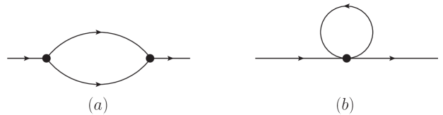
Figure 1: The topologies of 1PI graphs contributing to the two point function at 1-loop.

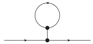
Figure 2: The tadpole topology of the graph contributing to the two point function at 1-loop. The bubble is fermionic and it is connected to the propagator by a zero-momentum $\tilde{\phi}$ line.

Below we shall use the following notation for the 1-loop integrals:

$${\rm I}[m^{2}]=\int\frac{d^{2}q}{(2\pi)^{2}}\frac{1}{q^{2}+m^{2}}\ ,$$ (3.2)

and

$$G[m_{1}^{2},m_{2}^{2};p^{2}]=\int\frac{d^{2}q}{(2\pi)^{2}}\frac{1}{(q^{2}+m_{1}^{2})((p-q)^{2}+m_{2}^{2})}=\frac{1}{4\pi}\int_{0}^{1}dx\frac{1}{p^{2}x(1-x)+m_{1}^{2}x+m_{2}^{2}(1-x)}\,.$$ (3.3)

The latter is UV finite and equal to

$$G[m_{1}^{2},m_{2}^{2};p^{2}]=\frac{\ln\ \frac{p^{2}+m_{1}^{2}+m_{2}^{2}+\sqrt{(p^{2}+m_{1}^{2}+m_{2}^{2})^{2}-4m_{1}^{2}m_{2}^{2}}}{p^{2}+m_{1}^{2}+m_{2}^{2}-\sqrt{(p^{2}+m_{1}^{2}+m_{2}^{2})^{2}-4m_{1}^{2}m_{2}^{2}}}}{4\pi\sqrt{(p^{2}+m_{1}^{2}+m_{2}^{2})^{2}-4m_{1}^{2}m_{2}^{2}}}\,.$$ (3.4)

In particular, we find that ($|p|=\sqrt{p^{2}}$)

$$G[m^{2},m^{2};p^{2}]=\frac{{\rm arcsinh}\frac{|p|}{2m}}{\pi\ |p|\sqrt{p^{2}+4m^{2}}}\,.$$ (3.5)

3.1 The $m=\sqrt{2}$ bosons

Let us start from the correction to the $\tilde{x}\tilde{x}^{*}$ 2-point function, which is the one involving the smaller number of diagrams due to the simplicity of the relevant vertices. The purely bosonic contribution to the 1-loop correction is

$$\langle\tilde{x}(p)\tilde{x}^{*}(-p)\rangle_{1}^{\rm bose}=\left(\frac{2\pi}{\sqrt{\lambda}}\right)^{2}\,32\frac{p_{1}^{2}+1}{(p^{2}+2)^{2}}\left[\int\frac{d^{2}q}{(2\pi)^{2}}\frac{(p_{1}-q_{1})^{2}+1}{(q^{2}+4)((p-q)^{2}+2)}-\frac{1}{2}\int\frac{d^{2}q}{(2\pi)^{2}}\frac{1}{q^{2}+4}\right]\,.$$ (3.6)

The first term here arises from the 3-vertex $\tilde{x}\tilde{x}^{*}\tilde{\phi}$, while the second one from the 4-vertex $\tilde{x}\tilde{x}^{*}\tilde{\phi}^{2}$.

The contributions involving fermions come from the 3-vertex $\tilde{x}\tilde{\eta}_{i}\tilde{\eta}^{j}$ and from the diagram in Fig. 2 obtained by attaching the $\tilde{\phi}$ tadpole to the propagator using the $\tilde{x}\tilde{x}^{*}\tilde{\phi}$ vertex. The sum of the two diagrams read

$$\langle\tilde{x}(p)\tilde{x}^{*}(-p)\rangle_{1}^{\rm fermi}=\left(\frac{2\pi}{\sqrt{\lambda}}\right)^{2}\,32\frac{p_{1}^{2}+1}{(p^{2}+2)^{2}}\left[\int\frac{d^{2}q}{(2\pi)^{2}}\frac{(q_{0}-p_{0})q_{0}}{(q^{2}+1)((p-q)^{2}+1)}-\int\frac{d^{2}q}{(2\pi)^{2}}\frac{q_{1}^{2}+1}{q^{2}+1}\right]\,.$$ (3.7)

One can see that the purely bosonic part eq. (3.6) and the fermionic part eq. (3.7) are separately free of logarithmic UV divergences. In (3.7), the tadpole contribution is important to achieve this.

The 1-loop integrals above may be evaluated in several different ways. We will choose to first perform a tensor reduction of the numerator factors, as described, for example, in the Appendix of [16]. We find

$$\langle\tilde{x}(p)\tilde{x}^{*}(-p)\rangle_{1}^{\rm bose}=\left(\frac{2\pi}{\sqrt{\lambda}}\right)^{2}\,\frac{p_{1}^{2}+1}{(p^{2}+2)^{2}}\Bigg{[}\frac{8}{{(p^{2})^{2}}}\left(\left(p^{2}+2\right)^{2}+4p^{2}\right)(p_{1}^{2}-p_{0}^{2})G[2,4;p^{2}]$$ (3.8)

$$~{}~{}~{}~{}~{}~{}~{}~{}~{}~{}~{}~{}~{}~{}~{}~{}~{}~{}~{}~{}~{}~{}~{}~{}~{}~{}~{}~{}~{}~{}~{}~{}~{}~{}~{}-\frac{8}{{(p^{2})^{2}}}\left(p^{2}+2\right)(p_{0}^{2}-p_{1}^{2})({\rm I}[4]-{\rm I}[2])\Bigg{]}$$ (3.9)

for the bosonic contribution and

$$\langle\tilde{x}(p)\tilde{x}^{*}(-p)\rangle_{1}^{\rm fermi}=\left(\frac{2\pi}{\sqrt{\lambda}}\right)^{2}\,\frac{p_{1}^{2}+1}{(p^{2}+2)^{2}}\Bigg{[}-\frac{8}{p^{2}}({(p^{2})^{2}}+4p_{1}^{2})G[1,1;p^{2}]\Bigg{]}$$ (3.10)

for the fermionic contribution.

Putting the two pieces together, the 1-loop correction to the $\tilde{x}\tilde{x}^{*}$ 2-point function is

$$\langle\tilde{x}(p)\tilde{x}^{*}(-p)\rangle_{1} = \left(\frac{2\pi}{\sqrt{\lambda}}\right)^{2}\frac{p_{1}^{2}+1}{(p^{2}+2)^{2}}\Bigg{[}\frac{8}{{(p^{2})^{2}}}\left(\left(p^{2}+2\right)^{2}+4p^{2}\right)(p_{1}^{2}-p_{0}^{2})G[2,4;p^{2}]$$ (3.12)

$$-\frac{8}{p^{2}}\left({(p^{2})^{2}}+4p_{1}^{2}\right)G[1,1;p^{2}]-\frac{8}{{(p^{2})^{2}}}\left(p^{2}+2\right)(p_{0}^{2}-p_{1}^{2})({\rm I}[4]-{\rm I}[2])\Bigg{]}$$

$$\equiv \left(\frac{2\pi}{\sqrt{\lambda}}\right)^{2}\frac{2}{(p^{2}+2)^{2}}\,F^{(1)}_{\tilde{x}\tilde{x}^{*}}(p_{0},p_{1})$$ (3.13)

Thus the resummed 2-point function in the 1-loop approximation is

$$\langle\tilde{x}(p)\tilde{x}^{*}(-p)\rangle=\frac{2\pi}{\sqrt{\lambda}}\ \frac{2}{p^{2}+2-\frac{2\pi}{\sqrt{\lambda}}F^{(1)}_{\tilde{x}\tilde{x}^{*}}(p_{0},p_{1})}\,.$$ (3.14)

The pole of the propagator is at $p^{2}=-2+{\cal O}(\frac{1}{\sqrt{\lambda}})$; therefore, to the 1-loop order we only need the “on-shell” value of $F^{(1)}_{\tilde{x}\tilde{x}^{*}}(p_{0},p_{1})$ which, using (3.4), i.e. $G[1,1;p^{2}=-2]=4G[2,4;p^{2}=-2]=\frac{1}{8}$, is simply

$$F^{(1)}_{\tilde{x}\tilde{x}^{*}}(p_{0},p_{1})|_{p^{2}=-2}=\frac{1}{2}\left(p_{1}^{2}+1\right)^{2}\,.$$ (3.15)

The 1-loop corrected dispersion relation for the 2 bosons of mass $m^{2}=2$ is then

$$p^{2}=-2+\frac{\pi}{\sqrt{\lambda}}\left(p_{1}^{2}+1\right)^{2}+{\cal O}(\frac{1}{\lambda})\,.$$ (3.16)

Wick-rotating to the Minkowski signature $(p_{0},p_{1})=(iE,p_{1})$, this gives the dispersion relation

$$E^{2}=p_{1}^{2}+2-\frac{\pi}{\sqrt{\lambda}}(p_{1}^{2}+1)^{2}+{\cal O}(\frac{1}{\lambda})$$ (3.17)

$$=\left(p_{1}^{2}+2-\frac{\pi}{\sqrt{\lambda}}\right)\left[1-\frac{\pi}{\sqrt{\lambda}}p_{1}^{2}\right]+{\cal O}(\frac{1}{\lambda})\,.$$ (3.18)

This precisely agrees with the result of [10].

3.2 The $m=2$ boson

Let us now consider the correction to the $\langle\tilde{\phi}\tilde{\phi}\rangle$ 2-point function. This calculation is especially interesting because this mode is absent in the analysis of [10].

Computing the relevant diagrams, one finds that the contributions corresponding to the topology involving two 3-vertices, Fig. 1$(a)$, are (below $s^{\alpha\beta}=$diag$(1,-1)$)

$$\langle\tilde{\phi}(p)\tilde{\phi}(-p)\rangle_{1}^{V_{3}V_{3}}=\left(\frac{2\pi}{\sqrt{\lambda}}\right)^{2}\frac{1}{(p^{2}+4)^{2}}\int\frac{d^{2}q}{(2\pi)^{2}}\Bigg{[}s^{\alpha\beta}s^{\gamma\delta}\frac{2q_{\alpha}q_{\gamma}(q_{\beta}q_{\delta}+2p_{\beta}q_{\delta}-3p_{\beta}p_{\delta})+4q_{\alpha}p_{\beta}p_{\gamma}p_{\delta}}{(q^{2}+4)((p-q)^{2}+4)}$$ (3.19)

$$~{}~{}~{}~{}~{}~{}~{}~{}~{}~{}~{}~{}~{}~{}~{}~{}~{}~{}~{}~{}~{}~{}~{}~{}~{}~{}~{}~{}~{}~{}~{}+16\frac{(q_{1}^{2}+1)((p_{1}-q_{1})^{2}+1)}{(q^{2}+2)((p-q)^{2}+2)}+10s^{\alpha\beta}s^{\gamma\delta}\frac{q_{\alpha}q_{\gamma}(p_{\beta}-q_{\beta})(p_{\delta}-q_{\delta})}{q^{2}(p-q)^{2}}$$ (3.20)

$$~{}~{}~{}~{}~{}~{}~{}~{}~{}~{}~{}~{}~{}~{}~{}~{}~{}~{}~{}~{}~{}~{}~{}~{}~{}~{}~{}~{}~{}~{}~{}-32\frac{((p_{1}-q_{1})^{2}+1)(q_{1}^{2}+1+q_{0}(p_{0}-q_{0}))}{(q^{2}+1)((p-q)^{2}+1)}\Bigg{]}\,.$$ (3.21)

Here the first two lines include all purely bosonic contributions, while the last line corresponds to the diagram with a fermion loop. The contributions to the graph in Fig. 1$(b)$ including the 4-vertex are

$$\langle\tilde{\phi}(p)\tilde{\phi}(-p)\rangle_{1}^{V_{4}} = \left(\frac{2\pi}{\sqrt{\lambda}}\right)^{2}\frac{1}{(p^{2}+4)^{2}}\int\frac{d^{2}q}{(2\pi)^{2}}\Bigg{[}-2\frac{q^{2}+4+p^{2}}{q^{2}+4}-16\frac{q_{1}^{2}+1}{q^{2}+2}-10\frac{q^{2}}{q^{2}}+32\frac{q_{1}^{2}+1}{q^{2}+1}\Bigg{]}$$ (3.22)

$$= \left(\frac{2\pi}{\sqrt{\lambda}}\right)^{2}\frac{1}{(p^{2}+4)^{2}}\int\frac{d^{2}q}{(2\pi)^{2}}\Bigg{[}-2\frac{p^{2}}{q^{2}+4}+16\frac{1}{q^{2}+1}\Bigg{]}\,.$$ (3.23)

Here in the second step we have dropped purely power-like divergences (using rotational invariance when needed). Finally, the tadpole diagram of Fig. 2 gives

$$\langle\tilde{\phi}(p)\tilde{\phi}(-p)\rangle_{1}^{\rm tad.}=\left(\frac{2\pi}{\sqrt{\lambda}}\right)^{2}\,8\frac{p_{0}^{2}-p_{1}^{2}}{(p^{2}+4)^{2}}\int\frac{d^{2}q}{(2\pi)^{2}}\frac{q_{1}^{2}+1}{q^{2}+1}=\left(\frac{2\pi}{\sqrt{\lambda}}\right)^{2}\,4\frac{p_{0}^{2}-p_{1}^{2}}{(p^{2}+4)^{2}}\int\frac{d^{2}q}{(2\pi)^{2}}\frac{1}{q^{2}+1}\,.$$ (3.24)

While the integrals appearing in the $\langle x(p)x^{*}(-p)\rangle$ 2-point function could also be analyzed directly through a Feynman parametrization, this does not seem to be convenient for the integrals appearing in eq. (3.21). Tensor-reducing the numerator factors yields:

$$\langle\tilde{\phi}(p)\tilde{\phi}(-p)\rangle_{1}^{V_{3}V_{3}}=\left(\frac{2\pi}{\sqrt{\lambda}}\right)^{2}\frac{1}{(p^{2}+4)^{2}}\Bigg{[}\frac{2}{{(p^{2})^{2}}}(p^{2}+4)^{2}(p_{0}^{2}-p_{1}^{2})^{2}\,G[4,4;p^{2}]-8\,{{\rm I}}[4]$$ (3.25)

$$~{}~{}~{}~{}~{}~{}~{}~{}+\left((p^{2}+4)^{2}+64\left(\frac{p_{1}^{4}}{{(p^{2})^{2}}}-\frac{p_{1}^{2}}{p^{2}}\right)\right)\,G[2,2;p^{2}]-2(4+p^{2})\,{{\rm I}}[2]$$ (3.26)

$$~{}~{}~{}~{}~{}~{}~{}~{}-4\frac{p_{1}^{2}}{{(p^{2})^{2}}}(p^{2}+4)({(p^{2})^{2}}+4p_{1}^{2})G[1,1;p^{2}]+8p_{1}^{2}{{\rm I}}[1]\Bigg{]}$$ (3.27)

Summing up the contributions in eq. (3.23),(3.24) and (3.27) we see that all UV divergences cancel out, since they combine into $2(p^{2}+4)\left(2{{\rm I}}[1]-{{\rm I}}[2]-{{\rm I}}[4]\right)=(p^{2}+4)\frac{3\ln 2}{2\pi}$. So the final result for the 1-loop correction to the $\tilde{\phi}$ propagator is

$$\langle\tilde{\phi}(p)\tilde{\phi}(-p)\rangle_{1}=\left(\frac{2\pi}{\sqrt{\lambda}}\right)^{2}\,\frac{1}{(p^{2}+4)^{2}}\Bigg{[}\frac{2}{{(p^{2})^{2}}}(p^{2}+4)^{2}(p_{0}^{2}-p_{1}^{2})^{2}\,G[4,4;p^{2}]$$

$$+\left((p^{2}+4)^{2}+64\left(\frac{p_{1}^{4}}{{(p^{2})^{2}}}-\frac{p_{1}^{2}}{p^{2}}\right)\right)\,G[2,2;p^{2}]-4\frac{p_{1}^{2}}{{(p^{2})^{2}}}(p^{2}+4)({(p^{2})^{2}}+4p_{1}^{2})G[1,1;p^{2}]+(p^{2}+4)\frac{3\ln 2}{2\pi}\Bigg{]}$$ (3.28)

$$\equiv\left(\frac{2\pi}{\sqrt{\lambda}}\right)^{2}\,\frac{1}{(p^{2}+4)^{2}}F^{(1)}_{\tilde{\phi}\tilde{\phi}}(p_{0},p_{1})$$ (3.29)

As we will discuss in detail in section 4, to obtain the corrected dispersion relation, it is sufficient as before to evaluate $F^{(1)}_{\tilde{\phi}\tilde{\phi}}(p_{0},p_{1})$ on-shell, i.e. at $p^{2}=-4$. From (3.4) one finds that

$$G[4,4;p^{2}=-4]=\frac{1}{24\sqrt{3}}\ ,\ \ \ \ \ \qquad G[2,2;p^{2}=-4]=\frac{1}{16}\,.$$ (3.30)

The third integral, $G[1,1;p^{2}=-4]$ diverges, since

$$G[1,1;p^{2}]=\frac{{\rm arcsinh}\frac{|p|}{2}}{\pi\ |p|\sqrt{p^{2}+4}}\ .$$ (3.31)

This integral corresponds to the graph in Fig. 1$(a)$ with a fermion loop and external $\tilde{\phi}$ field. The divergence can be attributed to the fact that due to the value of the masses, the $m=2$ boson may kinematically decay into a pair of on-shell $m=1$ fermions. However, the integral $G[1,1;p^{2}]$ appears in our result (3.29) multiplied by a factor $(p^{2}+4)$, and hence

$${\rm lim}_{p^{2}\rightarrow-4}\ \ (p^{2}+4)G[1,1;p^{2}]=0\ .$$ (3.32)

Therefore, due to dynamical reasons (the particular structure of the relevant cubic coupling in (2.24)), the fermionic loop contribution actually drops out of the on-shell self-energy. In section 4 we will see that, in contrast to the case considered in [15], the off-shell behavior of this term does not affect the existence of a real simple pole of the quantum corrected propagator due to the presence of other non-vanishing contributions. Indeed, we find that

$$F^{(1)}_{\tilde{\phi}\tilde{\phi}}(p_{0},p_{1})|_{p^{2}=-4}=\frac{1}{4}\,p_{1}^{2}(p_{1}^{2}+4)\,.$$ (3.33)

Then our final result is that the dispersion relation for $\tilde{\phi}$ at 1-loop is

$$p^{2}=-4+\frac{\pi}{2\sqrt{\lambda}}\,p_{1}^{2}(p_{1}^{2}+4)+{\cal O}(\frac{1}{\lambda})\,.$$ (3.34)

In Minkowski signature this gives

$$E^{2}=\left(p_{1}^{2}+4\right)\left[1-\frac{\pi}{2\sqrt{\lambda}}p_{1}^{2}\right]+{\cal O}(\frac{1}{\lambda})\,.$$ (3.35)

We observe that the mass, defined as the energy at zero momentum, does not receive corrections at 1-loop order, unlike the case of the $m=\sqrt{2}$ boson (cf. (3.17)).

3.3 The massless bosons

To conclude the analysis of bosonic fluctuations, let us consider the 1-loop propagator for the 5 massless fields $y^{a}$. The contributions from the topology in Fig. 1$(a)$ is

$$\langle y^{a}(p)y^{b}(-p)\rangle_{1}^{\rm V_{3}V_{3}}=\left(\frac{2\pi}{\sqrt{\lambda}}\right)^{2}\,\frac{\delta^{ab}}{{(p^{2})^{2}}}\int\frac{d^{2}q}{(2\pi)^{2}}\Bigg{[}\frac{4(p_{0}q_{0}-p_{1}q_{1})^{2}}{q^{2}((p-q)^{2}+4)}$$

$$\ \ \ \ \ \ \ \ \ \ \ \ \ \ \ \ \ +\ 8\frac{((p_{1}-q_{1})^{2}+1)(q_{1}^{2}+1-q_{0}(p_{0}-q_{0}))}{(q^{2}+1)((p-q)^{2}+1)}$$ (3.36)

$$\ \ \ \ \ \ \ \ \ \ \ \ \ \ \ \ +\ 4\frac{p_{0}^{2}q_{0}(p_{0}-q_{0})}{(q^{2}+1)((p-q)^{2}+1)}-16\frac{(q_{1}^{2}+1)p_{0}(p_{0}-q_{0})}{(q^{2}+1)((p-q)^{2}+1)}\Bigg{]}\,.$$ (3.37)

Here the first term in square brackets comes from the purely bosonic contribution, while the other three are due to fermions. We can now simplify these integrals by performing a tensor reduction of the numerators. To highlight the fact that the bosonic contribution is IR finite, we can make use of the identity ($G[m_{1}^{2},m_{2}^{2};p^{2}]$ was defined in (3.3))

$$G[0,m^{2};p^{2}]=\frac{1}{p^{2}+m^{2}}\left(\frac{1}{2\pi}\ln\frac{m^{2}+p^{2}}{m^{2}}-{{\rm I}}[m^{2}]+{{\rm I}}[0]\right)\,.$$ (3.38)

Then we have

$$\langle y^{a}(p)y^{b}(-p)\rangle_{1}^{\rm V_{3}V_{3}}=\left(\frac{2\pi}{\sqrt{\lambda}}\right)^{2}\frac{\delta^{ab}}{{(p^{2})^{2}}}\Bigg{[}\frac{1}{2\pi{(p^{2})^{2}}}(4+p^{2})({(p^{2})^{2}}-8p_{0}^{2}p_{1}^{2})\ln(1+\frac{p^{2}}{4})+2p^{2}{\rm I}[4]$$ (3.39)

$$~{}~{}~{}~{}~{}~{}~{}~{}~{}~{}~{}~{}~{}~{}~{}~{}~{}~{}~{}~{}~{}+\frac{4}{p^{2}}p_{0}^{2}({(p^{2})^{2}}+4p_{1}^{2})\,G[1,1;p^{2}]+(4-8p_{0}^{2}){{\rm I}}[1]\Bigg{]}\,.$$ (3.40)

The contributions coming from the 4-vertex are

$$\langle y^{a}(p)y^{b}(-p)\rangle_{1}^{\rm V_{4}}=\left(\frac{2\pi}{\sqrt{\lambda}}\right)^{2}\frac{\delta^{ab}}{{(p^{2})^{2}}}\int\frac{d^{2}q}{(2\pi)^{2}}\Bigg{[}\frac{5}{2}\frac{p^{2}}{q^{2}}-2\frac{p^{2}}{q^{2}+4}-8\frac{q_{1}^{2}+1}{q^{2}+1}\Bigg{]}$$ (3.41)

$$~{}~{}~{}~{}~{}~{}~{}~{}~{}~{}~{}~{}~{}~{}~{}~{}~{}~{}=\left(\frac{2\pi}{\sqrt{\lambda}}\right)^{2}\frac{\delta^{ab}}{{(p^{2})^{2}}}\Bigg{[}\frac{5}{2}p^{2}{{\rm I}}[0]-2p^{2}{{\rm I}}[4]-4{{\rm I}}[1]\Bigg{]}\,.$$ (3.42)

Finally, the contribution of the diagram involving the tadpole is

$$\langle y^{a}(p)y^{b}(-p)\rangle_{1}^{\rm tad.}=\left(\frac{2\pi}{\sqrt{\lambda}}\right)^{2}\frac{\delta^{ab}}{{(p^{2})^{2}}}\int\frac{d^{2}q}{(2\pi)^{2}}4\frac{p_{0}^{2}-p_{1}^{2}}{q^{2}+1}=\left(\frac{2\pi}{\sqrt{\lambda}}\right)^{2}\frac{\delta^{ab}}{{(p^{2})^{2}}}4(p_{0}^{2}-p_{1}^{2}){{\rm I}}[1]\,.$$ (3.43)

Summing everything up, we get

$$\langle y^{a}(p)y^{b}(-p)\rangle_{1}=\left(\frac{2\pi}{\sqrt{\lambda}}\right)^{2}\frac{\delta^{ab}}{{(p^{2})^{2}}}\Bigg{[}\frac{1}{2\pi{(p^{2})^{2}}}(4+p^{2})({(p^{2})^{2}}-8p_{0}^{2}p_{1}^{2})\ln\left(1+\frac{p^{2}}{4}\right)$$ (3.44)

$$~{}~{}~{}~{}~{}~{}+\frac{4}{p^{2}}p_{0}^{2}({(p^{2})^{2}}+4p_{1}^{2})\,G[1,1;p^{2}]-4p^{2}{{\rm I}}[1]+\frac{5}{2}p^{2}{{\rm I}}[0]\Bigg{]}\equiv\left(\frac{2\pi}{\sqrt{\lambda}}\right)^{2}\frac{\delta^{ab}}{{(p^{2})^{2}}}F^{(1)}_{yy}(p_{0},p_{1})\,.$$ (3.45)

To obtain the corrected dispersion relation, we again need to evaluate $F^{(1)}_{yy}(p_{0},p_{1})$ on-shell, i.e. at $p^{2}=0$, or $p_{0}^{2}=-p_{1}^{2}$. Then all of the UV and IR divergences in the result drop out. Using that at small $p^{2}$ we have $G[1,1;p^{2}]=\frac{1}{4\pi}-\frac{p^{2}}{24\pi}+\ldots$, and taking the limit $p_{0}^{2}\rightarrow-p_{1}^{2}$ in the above expression, we obtain

$$F^{(1)}_{yy}(p_{0},p_{1}){|_{p_{0}^{2}\rightarrow-p_{1}^{2}}}=\frac{7}{6\pi}p_{1}^{4}\,.$$ (3.46)

Notice that in the limit $p_{0}^{2}\rightarrow-p_{1}^{2}$ there is a cancellation of singular terms between the bosonic and fermionic contributions. Using this on-shell value, we conclude that the 1-loop corrected dispersion relation for the 5 massless fields is

$$p^{2}=\frac{7}{3\sqrt{\lambda}}p_{1}^{4}+{\cal O}(\frac{1}{\lambda})\,.$$ (3.47)

Going to Minkowski signature $(p_{0},p_{1})=(iE,p_{1})$, this gives the dispersion relation

$$E^{2}=p_{1}^{2}\left(1-\frac{7}{3\sqrt{\lambda}}p_{1}^{2}\right)+{\cal O}(\frac{1}{\lambda})\,.$$ (3.48)

3.4 The fermions

Let us finally look at the 1-loop correction to the 2-point function of the 8 fermionic fluctuations. The intermediate expressions for the various diagrams are much more involved in this case, and therefore we will omit most of the details here.

From the explicit 1-loop calculation, one can see that the non-vanishing entries in the fermion 2-point function matrix remain the same ones as at the tree level (2.20). In fact, the 1-loop corrections to the fermionic propagators can be written in the form

$$\langle\tilde{\theta}^{i}(p)\tilde{\eta}^{j}(-p)\rangle_{1}=-\left(\frac{2\pi}{\sqrt{\lambda}}\right)^{2}\frac{p_{1}-\mathrm{i}}{(p^{2}+1)^{2}}(\rho_{6}^{\dagger})^{ij}\,F^{(1)}_{\tilde{\theta}\tilde{\eta}}(p_{0},p_{1})\ ,$$ (3.49)

$$\langle\tilde{\theta}_{i}(p)\tilde{\eta}_{j}(-p)\rangle_{1}=-\left(\frac{2\pi}{\sqrt{\lambda}}\right)^{2}\frac{p_{1}-\mathrm{i}}{(p^{2}+1)^{2}}\rho^{6}_{ij}\,F^{(1)}_{\tilde{\theta}\tilde{\eta}}(p_{0},p_{1})$$ (3.50)

$$\langle\tilde{\theta}^{i}(p)\tilde{\theta}_{j}(-p)\rangle_{1}=-\left(\frac{2\pi}{\sqrt{\lambda}}\right)^{2}\frac{p_{0}}{(p^{2}+1)^{2}}\delta^{i}_{j}\,F^{(1)}_{\tilde{\theta}\tilde{\theta}^{\dagger}}(p_{0},p_{1})$$ (3.51)

$$\langle\tilde{\eta}^{i}(p)\tilde{\eta}_{j}(-p)\rangle_{1}=-\left(\frac{2\pi}{\sqrt{\lambda}}\right)^{2}\frac{p_{0}}{(p^{2}+1)^{2}}\delta^{i}_{j}\,F^{(1)}_{\tilde{\eta}\tilde{\eta}^{\dagger}}(p_{0},p_{1})\,.$$ (3.52)

Here $F^{(1)}_{\tilde{\theta}\tilde{\eta}},F^{(1)}_{\tilde{\theta}\tilde{\theta}^{\dagger}},F^{(1)}_{\tilde{\eta}\tilde{\eta}^{\dagger}}$ are $SU(4)$ scalars which are independent functions when momenta are off-shell. However, it turns out that they coincide up to terms which vanish on-shell (i.e. at $p^{2}=-1$). Computing the relevant 1-loop diagrams, reducing them to scalar integrals and dropping terms which do not contribute on-shell, one indeed finds that

$$F^{(1)}_{\tilde{\theta}\tilde{\eta}}(p_{0},p_{1})|_{{}_{p^{2}=-1}}=F^{(1)}_{\tilde{\theta}\tilde{\theta}^{\dagger}}(p_{0},p_{1})|_{{}_{p^{2}=-1}}=F^{(1)}_{\tilde{\eta}\tilde{\eta}^{\dagger}}(p_{0},p_{1})|_{{}_{p^{2}=-1}}$$ (3.53)

$$=16p_{1}^{2}(1+p_{1}^{2})\,G[1,2;p^{2}]+4(1+p_{1}^{2})\left({{\rm I}}[4]+2{{\rm I}}[1]-\frac{5}{4}{{\rm I}}[0]\right)$$ (3.54)

$$~{}~{}+4(1+p_{1}^{2})\left(\frac{5}{4}{{\rm I}}[0]-{{\rm I}}[4]\right)$$ (3.55)

$$~{}~{}-8(1+p_{1}^{2}){{\rm I}}[1]\,,$$ (3.56)

where the terms in the three lines correspond respectively to the contributions of the diagram in Fig. 1$(a)$, Fig. 1$(b)$ and Fig. 2. Notice that the integral $G[1,4;p^{2}]$ turns out to be absent when restricting to on-shell momenta, and so does the finite part of the integral $G[1,0;p^{2}]$ (to extract the finite part, we can use the identity (3.38)). Summing up the contributions in the three lines above, we find that the UV and IR divergences cancel on-shell. Using that $G[1,2;p^{2}=-1]=1/16$ we are then left with

$$F^{(1)}_{\tilde{\theta}\tilde{\eta}}(p_{0},p_{1})|_{{}_{p^{2}=-1}}=F^{(1)}_{\tilde{\theta}\tilde{\theta}^{\dagger}}(p_{0},p_{1})|_{{}_{p^{2}=-1}}=F^{(1)}_{\tilde{\eta}\tilde{\eta}^{\dagger}}(p_{0},p_{1})|_{{}_{p^{2}=-1}}=p_{1}^{2}(1+p_{1}^{2})\,.$$ (3.57)

Inserting this into the 1-loop propagators in (3.52) and comparing to the tree level expressions (2.20), we see that the effect of the 1-loop correction is to shift all denominators by the same amount

$$\frac{1}{p^{2}+1}\rightarrow\frac{1}{p^{2}+1-\frac{2\pi}{\sqrt{\lambda}}\,p_{1}^{2}(1+p_{1}^{2})}\,,$$ (3.58)

so that for all fermions we obtain the same dispersion relation (as expected by the $SO(6)$ symmetry)

$$p^{2}=-1+\frac{2\pi}{\sqrt{\lambda}}\,p_{1}^{2}(1+p_{1}^{2})+{\cal O}(\frac{1}{\lambda})\,.$$ (3.59)

In Minkowski signature this gives

$$E^{2}=\left(p_{1}^{2}+1\right)\left[1-\frac{2\pi}{\sqrt{\lambda}}\,p_{1}^{2}\right]+{\cal O}(\frac{1}{\lambda})\,,$$ (3.60)

which is again in agreement with the ABA result of [10].

4 Comments on poles of the 2-point function, physical states and stability

In the previous section we evaluated the 1-loop correction to the 2-point function of the worldsheet excitations around the long spinning string or, equivalently, the null cusp minimal surface. We carried out the computation on a Euclidean worldsheet; upon analytic continuation to 2d Lorentzian signature ($p_{0}\to iE$), the 1-loop corrections modify the dispersion relation of these excitation by shifting position of the pole of the tree-level 2-point functions. In general, depending on the precise structure of the 1-loop correction to the amputated 2-point function (“self-energy” operator) $\Pi(p_{0},p_{1};\lambda)$, the position of the real pole in the classical propagator may get shifted but it may also happen that the pole may disappear being replaced by a branch cut. In the latter case the corresponding field will no longer represent an asymptotic particle state, as was suggested in [15] for the heavier BMN field in string theory in $AdS_{4}\times\mathbb{CP}^{3}$. As we have seen, in our case the situation is different: all classical excitations, including the heaviest $AdS_{3}$ mode $\tilde{\phi}$, continue to exhibit poles in their quantum-corrected propagator. Let us discuss the difference with the example in [15] in more detail.

4.1 Existence of poles in the 2-point function

Consider a field $\Phi$ with the classical mass-shell condition $p^{2}+m^{2}=0$ and the quantum-corrected 2-point function having a generic form ($p^{2}=p_{0}^{2}+p_{1}^{2}=-E^{2}+p_{1}^{2}$)

$$\langle\Phi(p)\Phi(-p)\rangle=\frac{1}{p^{2}+m^{2}-\Pi(p_{0},p_{1};\lambda)}\ ,\ \ \ \ \ \ \ \ \ \ \ \ \ \ \Pi(p_{0},p_{1};\lambda)={\textstyle{2\pi\over{\sqrt{\lambda}}}}F^{(1)}(p_{0},p_{1})+{\cal O}({\textstyle{1\over({\sqrt{\lambda}})^{2}}})\ ,$$ (4.1)

where we assumed that the theory is such that, like in (2.24),(2.29), the interaction terms do not in general preserve 2d Lorentz invariance. The corrected dispersion relation is then determined by the real solutions of $p^{2}+m^{2}-\Pi(p_{0},p_{1};\lambda)=0$. As usual, the existence of a real simple pole of the exact propagator is equivalent to the possibility to identify the excitations of the field $\Phi$ as free asymptotic particles.

Let us further assume that the 1-loop term in $\Pi$ has the following form

$$F^{(1)}(p_{0},p_{1})=a_{0}+a_{1/2}(p^{2}+m^{2})^{1/2}+a_{1}(p^{2}+m^{2})+a_{2}(p^{2}+m^{2})^{2}\ ,\ \ \ \ \ \ \ \ \ \ a_{k}=a_{k}(p_{0},p_{1})\ ,$$ (4.2)

where the coefficients $a_{k}$ should be regular at $p^{2}=-m^{2}$. This is actually the structure we have found in (3.29) (and also in (3.13) and (3.45) and the off-shell fermion 2-point function; in these cases $a_{1/2}=0$). The non-analytic $(p^{2}+m^{2})^{1/2}$ term appears in the propagator of the $AdS_{3}$ mode $\tilde{\phi}$ and also in the case of the heavy BMN mode in [15] due to the possibility of a threshold two-body decay of the field of mass $m$ into two fields of mass ${\textstyle{1\over 2}}m$ present in the theory.

In the case considered in [15] it was conjectured that due to underlying supersymmetry the leading coefficient $a_{0}$ should vanish so that the non-trivial part of $F^{(1)}$ close to the original mass shell is essentially determined by the threshold term,

$$F^{(1)}(p_{0},p_{1})_{{}_{AdS_{4}\times\mathbb{CP}^{3}}}=a_{1/2}(p^{2}+m^{2})^{1/2}+{\cal O}(p^{2}+m^{2})\ ,\ \ \ \ \ \ \ \ \ \ \ \ \ \ a_{1/2}=-{1\over 4\pi}p^{2}_{1}\ ,$$ (4.3)

where the value of $a_{1/2}$ was found [15] by the explicit 1-loop computation. In this case the condition for existence of a pole in the propagator (4.1) may be written as

$$-E^{2}+p_{1}^{2}+m^{2}-{2\pi\over{\sqrt{\lambda}}}a_{1/2}(-E^{2}+p_{1}^{2}+m^{2})^{1/2}={\cal O}({\textstyle{1\over({\sqrt{\lambda}})^{2}}})\ ,$$ (4.4)

i.e. for $E\approx e(p_{1})+{\cal O}({\textstyle{1\over{\sqrt{\lambda}}}})$ where $e(p_{1})\equiv\sqrt{p_{1}^{2}+m^{2}}$ we get

$$E-e(p_{1})+{2\pi\ {a_{1/2}}\over{\sqrt{\lambda}}\ \sqrt{2e(p_{1})}}\sqrt{e(p_{1})-E}\ ={\cal O}({\textstyle{1\over({\sqrt{\lambda}})^{2}}})\ .$$ (4.5)

This equation does not have a solution $E=e(p_{1})+{\cal O}({\textstyle{1\over({\sqrt{\lambda}})^{2}}})$ for a real pole in $E$ since $a_{1/2}<0$. The resulting conclusion of [15] was that in such case the particle of mass $m$ dissolves in the continuum of 2-particle states of field of mass ${\textstyle{1\over 2}}m$, i.e. it does not exist as an asymptotic state in the spectrum at finite $\lambda$.

The main difference of this case compared to our analysis of the propagator of the $\tilde{\phi}$ mode with $m^{2}=4$ is that here $a_{0}\not=0$ in (3.29), i.e. $F^{(1)}_{\tilde{\phi}\tilde{\phi}}|_{{}_{p^{2}=-m^{2}}}=a_{0}\not=0$ (see (3.33)). As a result, the real pole of the corrected propagator is readily found and was already given in (3.35). Indeed, we find (cf. (4.4),(4.5))

$$-E^{2}+p_{1}^{2}+m^{2}-{2\pi\over{\sqrt{\lambda}}}a_{0}={\cal O}({\textstyle{1\over({\sqrt{\lambda}})^{2}}})\ ,$$ (4.6)

$$E=e(p_{1})-{\pi\over{\sqrt{\lambda}}}{a_{0}\over e(p_{1})}+{\cal O}({\textstyle{1\over({\sqrt{\lambda}})^{2}}})=e(p_{1})\Big{[}1-{\pi\over 4{\sqrt{\lambda}}}p^{2}_{1}\Big{]}+{\cal O}({\textstyle{1\over({\sqrt{\lambda}})^{2}}})\ ,$$ (4.7)

which is equivalent to (3.35) for $a_{0}={1\over 4}p^{2}_{1}[e(p_{1})]^{2}$ in (3.33). As a result, this heavy $AdS_{3}$ mode remains an asymptotic state in the spectrum. The same analysis applies also to all the other excitations we discussed in section 3 (which also have $a_{0}\not=0$ in their self-energy operator) leading to the dispersion relations in (3.17), (3.48) and (3.60).

As a remark, let us however note that there is still a possible scenario in which a slightly modified version of the argument of [15] described above appears to apply. Suppose that the denominator of the all-loop resummed 2-point function takes the form

$$p^{2}+m^{2}-\Pi(p_{0},p_{1};\lambda)=\Delta-\frac{2\pi}{{\sqrt{\lambda}}}\ {\rm a}_{1/2}\ \Delta^{1/2}-\frac{2\pi}{{\sqrt{\lambda}}}\sum_{k\geq 1}{\rm a}_{k}\ \Delta^{k}$$ (4.8)

$$\Delta\equiv p^{2}+\tilde{m}^{2}(p_{0},p_{1};{\sqrt{\lambda}})\ ,\ \ \ \ \ \ \ \ \ \tilde{m}^{2}(p_{0},p_{1};{\sqrt{\lambda}})=m^{2}-\frac{2\pi}{{\sqrt{\lambda}}}\ {\rm a}_{0}(p_{0},p_{1};{\sqrt{\lambda}})\ ,$$

$${\rm a}_{r}\equiv{\rm a}_{r}(p_{0},p_{1};{\sqrt{\lambda}})=a_{r}(p_{0},p_{1})+{\cal O}(\frac{1}{{\sqrt{\lambda}}})\,,\ \ \ \ \ \ \ \ \ \ r=0,1/2,1,...$$

Note that this structure is, in principle, compatible with our 1-loop result for $\langle\tilde{\phi}(p)\tilde{\phi}(-p)\rangle$. Expanding in powers of $\frac{1}{\sqrt{\lambda}}$, one would find a pole to any order in perturbation theory, in particular reproducing the 1-loop dispersion relation as described above. However, the zero of the exact denominator at $p^{2}=-\tilde{m}^{2}$ does not yield a simple pole of the 2-point function but just a branch cut due to the square root term. Therefore, as in [15], one may be led to the conclusion that the particle of mass $m$ dissolves in the continuum of two-particle states. While this is, in principle, a possibility we cannot rule out, we would like to stress that it relies on very strong assumptions regarding the analytic structure of the higher loop corrections to the 2-point function, which, in the absence of explicit calculations, appear to be not very well motivated. It would be interesting to explore this further by examining, e.g., the 2-loop corrections to the propagator.

It is interesting to further discuss the consequences of the presence of the non-analytic term

$$F^{(1)}_{\tilde{\phi}\tilde{\phi}}(p_{0},p_{1})=a_{1/2}(p^{2}+4)^{1/2}+\ldots$$ (4.9)

in the 1-loop self-energy for the field $\tilde{\phi}$ at higher orders in perturbation theory in $1\over{\sqrt{\lambda}}$. Here the explicit value of $a_{1/2}$ can be read off from eq. (3.29) and the omitted terms are analytic close to the mass-shell. When solving perturbatively for the poles of the quantum corrected 2-point function, one would need to evaluate $F^{(1)}_{\tilde{\phi}\tilde{\phi}}(p_{0},p_{1})$ at the position of the 1-loop corrected pole. According to eq. (3.34),(4.6), this is given by $p^{2}+4=\frac{\pi}{2\sqrt{\lambda}}p_{1}^{2}(p_{1}^{2}+4)\geq 0$, i.e. the energy $E$ in (4.7) is shifted below the threshold, $E-e(p_{1})\,{\leqslant}\,0$. Therefore, the 1-loop self-energy remains real on the 1-loop corrected mass shell which is consistent with our conclusion that $\tilde{\phi}$ represents a stable asymptotic state in the spectrum (the presence of an imaginary part would imply a non-vanishing decay width, see the next subsection).

We notice, at the same time, that the presence of the square root term in (4.9) introduces a potential non-analyticity in the on-shell value of the self-energy of $\tilde{\phi}$ considered as a function of $\sqrt{\lambda}$ and $p_{1}$. Indeed,

$$(p^{2}+4)^{1/2}|_{{}_{p^{2}+4=\frac{\pi}{2\sqrt{\lambda}}p_{1}^{2}(p_{1}^{2}+4)}}\ \sim\ \lambda^{-1/4}\sqrt{p_{1}^{2}(p_{1}^{2}+4)}\,.$$ (4.10)

As a result, the next to the leading correction in the dispersion relation (4.7) would actually be of order ${\textstyle{1\over\lambda^{3/4}}}$ instead of the expected ${\cal O}({\textstyle{1\over({\sqrt{\lambda}})^{2}}})$ one. It is possible that this non-analytic behavior, which would single out $\tilde{\phi}$ as being very different from the other fluctuation fields, may be compensated by suitable contributions to the 2-loop self-energy $F^{(2)}_{\tilde{\phi}\tilde{\phi}}(p_{0},p_{1})$. Once again, an explicit 2-loop calculation appears to be needed in order to settle this question.

4.2 On higher-order stability of the $m=2$ field

The field ${\tilde{\phi}}$ is kinematically allowed to decay into a pair of fermions and the relevant interaction terms are present in the Lagrangian (2.13). The existence of this decay becomes therefore a dynamical question. As we have seen above, the poles of the 1-loop corrected 2-point function are real. The absence of an imaginary part at this order implies that ${\tilde{\phi}}$ has vanishing decay width $\Gamma$ at the tree-level. Indeed, the two are related via the optical theorem

$$\Gamma=\frac{1}{m}{\rm Im}\ \Pi|_{{}_{p^{2}=-m^{2}}}\ ,\$$ (4.11)

where in the present case $m^{2}=4$ and $\Pi={2\pi\over{\sqrt{\lambda}}}F_{\tilde{\phi}\tilde{\phi}}^{(1)}(p_{0},p_{1})+...$ is the sum of all quantum corrections to the amputated on-shell 2-point function. The knowledge of $n$-loop corrections to $\Pi$ thus allows one to deduce the $(n-1)$-loop decay width. Since, as was already discussed, the on-shell 1-loop 2-point function found in section 3.2 is real, the total tree-level decay width vanishes.

Reversing the logic of the optical theorem and further using the generalized unitarity to disentangle various multi-particle decay channels, we can gain information about the 1-loop stability of the ${\tilde{\phi}}$ field. Indeed, the complete imaginary part may be evaluated as the on-shell limit of the unitarity cut of the off-shell 2-point function. At the 1-loop level, see Fig. 3$(a)$, this is nothing but the product of certain on-shell tree-level vertices and two cut propagators (i.e. the residues of Feynman propagators at the positive energy poles). At the 2-loop level, the unitarity cut receives two types of contributions: two-particle cuts shown in Fig. 3$(b)$, and three-particle cuts shown in Fig. 3$(c)$. Through the generalized unitarity method (see, e.g., [22, 12] and references therein) these two contributions may be computed and interpreted separately. Each of these two contributions is responsible for one decay channel: Fig. 3$(b)$ contains contributions to a two-particle final state while Fig. 3$(c)$ contains contributions to a three-particle final state.

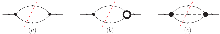
Figure 3: Unitarity cuts at one and two loops. In figure $(b)$ the right hand side part denotes a 1-loop vertex correction. The black dots in figure $(c)$ represent on-shell 4-point amplitudes, which receive contributions from the 4-point vertices as well as from the two three-point vertices.

By analyzing the 1-loop unitarity cut it is easy to see that the product between the ${\tilde{\phi}}{\tilde{\eta}}{\tilde{\theta}}$ 3-point vertex (the second line of (2.24)) and two-cut fermion propagators is proportional to $(p^{2}+4)^{1/2}$ where $p$ is the momentum of ${\tilde{\phi}}$; it thus vanishes for an on-shell field. This shows that the appearance of the similar factor arising from $(p^{2}+4)G[1,1;p^{2}]$ in $\langle{\tilde{\phi}}(p){\tilde{\phi}}(-p)\rangle$ does not rely on summing over all fermionic degrees of freedom.

This observation has an immediate consequence for the part of the cut of the 2-loop 2-point function that describes the decay of ${\tilde{\phi}}$ into two fermions, Fig. 3$(b)$. Indeed, this cut as well as the one in which the vertex correction is on the left side of the cut are proportional to the same product of the ${\tilde{\phi}}{\tilde{\eta}}{\tilde{\theta}}$ 3-point vertex and two-cut fermion propagators and therefore vanish on shell. Consequently, the 1-loop partial decay width into two fermions vanishes.

The analysis of the three-particle cut 3$(c)$ is more involved and will not be attempted here. It is possible that the most efficient way to extract it is from the 2-loop expression for the 2-point function which would be interesting to compute.

5 Concluding remarks

In this paper we used superstring sigma model perturbation theory to compute the leading strong-coupling corrections to the dispersion relations of the fluctuation modes near the long spinning string in $AdS_{5}$ and compared the results with the asymptotic Bethe ansatz predictions [10].

There are several directions that may be interesting to explore. One is extending our computation to the 2-loop level with a possibility of further comparison to the corresponding terms in ABA [10]. That would also check our unitarity-based arguments about the stability of the heaviest $AdS_{3}$ mode $\tilde{\phi}$. Such 2-loop computation would be similar in spirit to a 3-loop computation of the cusp anomaly and at the moment appears to be technically challenging.

Also interesting would be the analysis of multi-excitations/bound states and the computation of the scattering matrix for all the fluctuations. Such a calculation would potentially access the higher-twist excitations discussed in [10] and provide further detailed tests of the ABA.

Another generalization is to the case of non-zero angular momentum in $S^{5}$, which should allow to determine corrections to the dispersion relations in (1.8),(1.8). As discussed in the introduction, that may also help clarify the fate of the heaviest excitation mode.

Finally, it would be interesting to apply direct string sigma model techniques developed in [16, 17] and here to the computation of strong-coupling corrections to the null polygonal Wilson loops via the OPE approach of [11].

Acknowledgments
We would like to thank F. Alday and J. Maldacena for raising the interesting question about superstring corrections to the excitation spectrum of the long spinning string that motivated this investigation. We also acknowledge helpful discussions with J. Collins, P. Vieira and D. Volin. We are grateful to B. Basso and K. Zarembo for very useful comments on the first version of this paper. This work was supported in part by the US National Science Foundation under PHY-0855356 (R.Ro.), the US Department of Energy under contracts DE-FG02-201390ER40577 (OJI) (R.Ro.) and the A.P. Sloan Foundation (R.Ro.). It was also supported by EPSRC (R.Ri.). The work of S.G. is supported by Perimeter Institute for Theoretical Physics. Research at Perimeter Institute is supported by the Government of Canada through Industry Canada and by the Province of Ontario through the Ministry of Research $\&$ Innovation.

References

• [1] S. S. Gubser, I. R. Klebanov and A. M. Polyakov, “A semi-classical limit of the gauge/string correspondence,” Nucl. Phys.  B 636 (2002) 99 [arXiv:hep-th/0204051].
• [2] H. J. de Vega and I. L. Egusquiza, “Planetoid String Solutions in 3 + 1 Axisymmetric Spacetimes,” Phys. Rev.  D 54, 7513 (1996) [arXiv:hep-th/9607056].
• [3] S. Frolov and A. A. Tseytlin, “Semiclassical quantization of rotating superstring in AdS(5) x S(5),” JHEP 0206 (2002) 007 [arXiv:hep-th/0204226].
• [4] S. Frolov, A. Tirziu and A. A. Tseytlin, “Logarithmic corrections to higher twist scaling at strong coupling from AdS/CFT,” Nucl. Phys.  B 766, 232 (2007) [arXiv:hep-th/0611269].
• [5] M. Kruczenski, “A note on twist two operators in N = 4 SYM and Wilson loops in Minkowski signature,” JHEP 0212, 024 (2002) [arXiv:hep-th/0210115].
• [6] L. F. Alday and J. M. Maldacena, “Gluon scattering amplitudes at strong coupling,” JHEP 0706, 064 (2007) [arXiv:0705.0303].
• [7] M. Kruczenski, R. Roiban, A. Tirziu and A.A. Tseytlin, “Strong-coupling expansion of cusp anomaly and gluon amplitudes from quantum open strings in $AdS_{5}\times S^{5}$,” Nucl. Phys.  B 791, 93 (2008) [arXiv:0707.4254].
• [8] L. F. Alday and J. M. Maldacena, “Comments on operators with large spin,” JHEP 0711 (2007) 019 [arXiv:0708.0672].
• [9] D. Gaiotto, J. Maldacena, A. Sever and P. Vieira, “Bootstrapping Null Polygon Wilson Loops,” arXiv:1010.5009 .
• [10] B. Basso, “Exciting the GKP string at any coupling,” arXiv:1010.5237 .
• [11] L. F. Alday, D. Gaiotto, J. Maldacena, A. Sever and P. Vieira, “An Operator Product Expansion for Polygonal null Wilson Loops,” arXiv:1006.2788
• [12] L. F. Alday and R. Roiban, “Scattering Amplitudes, Wilson Loops and the String/Gauge Theory Correspondence,” Phys. Rept.  468, 153 (2008) [arXiv:0807.1889].
• [13] N. Beisert, B. Eden and M. Staudacher, “Transcendentality and crossing,” J. Stat. Mech.  0701, P021 (2007) [arXiv:hep-th/0610251].
• [14] N. Dorey and M. Losi, “Giant Holes,” J. Phys. A 43 (2010) 285402 [arXiv:1001.4750]; “Spiky Strings and Giant Holes,” arXiv:1008.5096 .
• [15] K. Zarembo, “Worldsheet spectrum in AdS(4)/CFT(3) correspondence,” JHEP 0904, 135 (2009) [arXiv:0903.1747].
• [16] S. Giombi, R. Ricci, R. Roiban, A. A. Tseytlin and C. Vergu, “Generalized scaling function from light-cone gauge $AdS_{5}\times S^{5}$ superstring,” JHEP 1006, 060 (2010) [arXiv:1002.0018]. “Quantum $AdS_{5}\times S^{5}$ superstring in the AdS light-cone gauge,” JHEP 1003, 003 (2010) [arXiv:0912.5105].
• [17] S. Giombi, R. Ricci, R. Roiban and A. A. Tseytlin, “Two-loop $AdS_{5}\times S^{5}$ superstring: testing asymptotic Bethe ansatz and finite size corrections,” arXiv:1010.4594 .
• [18] R. R. Metsaev, C. B. Thorn and A. A. Tseytlin, “Light-cone superstring in AdS space-time,” Nucl. Phys.  B 596, 151 (2001) [arXiv:hep-th/0009171]. R. R. Metsaev and A. A. Tseytlin, “Superstring action in AdS(5) x S(5): kappa-symmetry light cone gauge,” Phys. Rev.  D 63, 046002 (2001) [arXiv:hep-th/0007036].
• [19] M. Beccaria, G. V. Dunne, V. Forini, M. Pawellek and A. A. Tseytlin, “Exact computation of one-loop correction to energy of spinning folded string in $AdS_{5}\times S^{5}$ ,” J. Phys. A 43, 165402 (2010) [arXiv:1001.4018].
• [20] R.R. Metsaev and A.A. Tseytlin, “Type IIB superstring action in AdS(5) x S(5) background,” Nucl. Phys.  B 533, 109 (1998) [arXiv:hep-th/9805028].
• [21] N. Gromov and P. Vieira, “Complete 1-loop test of AdS/CFT,” JHEP 0804, 046 (2008) [arXiv:0709.3487]. P. Y. Casteill and C. Kristjansen, “The Strong Coupling Limit of the Scaling Function from the Quantum String Bethe Ansatz,” Nucl. Phys.  B 785, 1 (2007) [arXiv:0705.0890]. B. Basso, G. P. Korchemsky and J. Kotanski, “Cusp anomalous dimension in maximally supersymmetric Yang-Mills theory at strong coupling,” Phys. Rev. Lett.  100, 091601 (2008) [arXiv:0708.3933]. N. Gromov, “Generalized Scaling Function at Strong Coupling,” JHEP 0811, 085 (2008) [arXiv:0805.4615].
• [22] Z. Bern, L. J. Dixon, D. C. Dunbar and D. A. Kosower, “One loop n point gauge theory amplitudes, unitarity and collinear limits,” Nucl. Phys. B 425, 217 (1994) [hep-ph/9403226]; R. Britto, F. Cachazo and B. Feng, “Generalized unitarity and one-loop amplitudes in N = 4 super-Yang-Mills,” Nucl. Phys.  B 725, 275 (2005) [hep-th/0412103]. Z. Bern, J. J. M. Carrasco, H. Johansson and D. A. Kosower, “Maximally supersymmetric planar Yang-Mills amplitudes at five loops,” Phys. Rev.  D 76, 125020 (2007) [0705.1864].