Built-up structure criticality

Abstract.

The built-up land represents an important type of an overall landscape. In this paper the built-up land structure in the largest cities in the Czech Republic and some selected cities in the U.S.A. is analyzed using the framework of statistical physics. We calculate the variance of the total area and of the count of the built-up land plots contained inside discs of different radii. In both cases the variance as a function of the disc radius follows a power law with exponents that are comparable through different cities. The study is based on the cadastral data from the Czech Republic and on the building footprints from GIS data in the U.S.A.

¹ Department of Physics, Faculty of Nuclear Sciences and Physical Engineering
Czech Technical University in Prague, Břehová 7, CZ-115 19, Prague, Czech Republic
² Doppler Institute for Mathematical Physics and Applied Mathematics
Faculty of Nuclear Sciences and Physical Engineering
Czech Technical University in Prague, Břehová 7, CZ-115 19, Prague, Czech Republic
³ Nuclear Physics Institute, Academy of Sciences of the Czech Republic
CZ-25068, Řež near Prague, Czech Republic
⁴ Faculty of Science, University of Hradec Králové, Víta Nejedlého 573
CZ-50002, Hradec Králové, Czech Republic

1. Introduction

Urban land represents one of the most significant fingerprints of human activity on the Earth. The creation and development of its structure is influenced by cultural, sociological, economic, political and other conditions. Despite the apparent complexity, some simple universal properties and rules were found. The classic example is the rank size distribution of cities firstly mentioned by Auerbach (in [1]) and later discussed by Zipf [2]. They claimed that if the cities are ranked by the number of inhabitants, then the rank-size distribution follows a power law with the exponent close to -1 (see also [3]).

From the physical point of view it is interesting to study spatial properties of the urban structure. Existing studies [1, 4, 5, 6, 7, 3, 8] focused especially on the fractal structure and the related scaling-laws of urban clusters. The analyzed pattern is usually given by some coarse-grained map of the spatial population spread and the general claim is that the spatial structure of large urban areas is influenced by certain long-range spatial correlations. Motivated by those properties several urban models were introduced [1, 4, 7, 9, 10, 11, 12].

Our aim here is to study the urban structure in a different representation and on much smaller scales. The analyzed data consists of the exact positions of buildings in the cities where we can expect the urbanization to be only slowly varying with time. The vertical projection of buildings onto the ground gives a built-up land pattern, that forms a natural representation of the city since it is clearly visible and identifiable. Built-up land is usually stable over short and medium time periods as days, months and even years, except of rapid changes during disasters. It is straightforward to expect that the built-up land pattern is correlated with population spread since the human live is strongly connected with buildings. The exact relation however can be rather complicated as it depends on many additional features like the whole 3D shape (capacity) or the usage (living, working) of every building and can in general vary during the day and over short time periods (weekends, vacations e.g.).

In this paper we show that the correlation and fluctuation properties of such built-up land pattern in the city centres are similar as those of the critical systems in thermodynamics. This can represent a connection between the urban and the critical systems. It can be especially helpful when discussing the self-organized criticality concept [13] that was for the urban system introduced by Batty and Xie [14] with a fractal dimension as the criticality indicator.

A connection to the critical systems (phase transitions) can originate from the fact that economically the change of a land to a built-up type represents a change of phase. The land acquires an additional property - a building.

2. Critical phenomena

Let us briefly recall the correlation and fluctuation properties typical for thermodynamic systems near the critical point (e.g. [15, 16, 17]). For a further discussion on the scaling properties in complex systems see [18].

The most important property of the static spacial structure of a critical system is its scaling invariance. In simple terms, if a part of the system is magnified to the same size as the original system, it is not possible to distinguish between the magnified part and the original system.

In order to describe these features explicitly let us define a local order parameter $m$ as a quantity that solely describes the microscopic state of the system in one realization. Thus $m(\boldsymbol{r})$ is the value of the parameter (e.g. density, local magnetization or boolean indicator of some property occurrence) at the position $\boldsymbol{r}\in V$, where $V\subset\mathbbm{R}^{2}$ is the total volume occupied by the 2-dimensional system living in the plane.

Suppose there exist a whole ensemble of realizations (different cities can be treated as different realizations) and denote by $\langle...\rangle$ the ensemble average. We say that the system is homogeneous and isotropic in the volume $V$, if

(1) $$\langle m(\boldsymbol{r})\rangle=\langle m(0)\rangle=m,\qquad\forall\boldsymbol{r}\in V.$$

This means that the mean value of the local order parameter is independent of position in the volume. From now we assume the system to be homogeneous and isotropic.

The spatial properties of the order parameter distribution can be described by the two-point correlation function defined as

(2) $$G(\boldsymbol{r}_{1},\boldsymbol{r}_{2})=\bigg{\langle}\Big{(}m(\boldsymbol{r}_{1})-\langle m(\boldsymbol{r}_{1})\rangle\Big{)}\Big{(}m(\boldsymbol{r}_{2})-\langle m(\boldsymbol{r}_{2})\rangle\Big{)}\bigg{\rangle}.$$

This is under homogeneity and isotropy assumptions simplified to

(3) $$G(\boldsymbol{r}_{1},\boldsymbol{r}_{2})=G(\boldsymbol{r}_{2}-\boldsymbol{r}_{1})=G(r)=\langle m(\boldsymbol{r})m(0)\rangle-m^{2},$$

where $\boldsymbol{r}=\boldsymbol{r}_{2}-\boldsymbol{r}_{1}$ and $r=\left|\boldsymbol{r}\right|$. Therefore the correlation function depends only on the relative distance $\left|\boldsymbol{r}\right|=\left|\boldsymbol{r}_{2}-\boldsymbol{r}_{1}\right|$ of the two points $\boldsymbol{r}_{1}$ and $\boldsymbol{r}_{2}$.

The scaling assumption for systems at the critical point can be written in the following form:

(4) $$G(r)\sim\frac{1}{r^{\eta}},\quad 0<\eta<2,$$

Index $\eta$ appearing in the exponent of the power law part of $G(r)$ is called the anomalous dimension. For systems outside the critical point the correlation function decays with increasing $r$ much faster (usually exponentially).

The definition of the order parameter can be extended to systems composed of point particles. Here, the empirical density function $\rho$ is taken as the local order parameter. For particles located at points $\boldsymbol{r}_{1},\ \boldsymbol{r}_{2},\ \boldsymbol{r}_{3},\ \boldsymbol{r}_{4},\ ...\in\mathbbm{R}^{2}$ it is given by

(5) $$\rho(\boldsymbol{r})=\sum_{i=1}^{\infty}\delta(\boldsymbol{r}-\boldsymbol{r}_{i}).$$

It is well known [17] that the correlation function for such density can be decomposed to

(6) $$G(\boldsymbol{r}_{2}-\boldsymbol{r}_{1})=\rho_{0}\delta(\boldsymbol{r}_{2}-\boldsymbol{r}_{1})+\mathcal{G}(\boldsymbol{r}_{2}-\boldsymbol{r}_{1}),$$

where $\mathcal{G}(\boldsymbol{r}_{2}-\boldsymbol{r}_{1})$ is the non-diagonal part of the form (4) defined for $r=\left|\boldsymbol{r}_{2}-\boldsymbol{r}_{1}\right|>0$. The difference to the ordinary order parameter is thus only in the diagonal $\delta$ therm which of course doesn’t influence the character of the divergence in the vicinity of the critical point.

2.1. Parameter variance in discs

An useful tool to analyze the experimental data is the variance of the parameter value inside discs. For the parameter $m(\boldsymbol{r})$ with homogeneous and isotropic distribution $\langle m(\boldsymbol{r})\rangle=m$ the cumulative value of the parameter in the disc of a radius $R$ is given by

(7) $$M(R)=\int_{S(R)}m(\boldsymbol{r})d\boldsymbol{r},$$

where the disc is the set $S(R)\equiv\{\boldsymbol{r}\in\mathbbm{R}^{2}|\left|\boldsymbol{r}\right|<R\}$ with a volume $\left|S(R)\right|$. The centre of the disc is not important due to the homogeneity of the parameter distribution. The parameter variance is defined [19] as

(8) $$\sigma^{2}(R)=\langle M(R)^{2}\rangle-\langle M(R)\rangle^{2},$$

where

(9) $$\langle M(R)\rangle=\int_{S(R)}\langle m(\boldsymbol{r})\rangle d\boldsymbol{r}=m\left|S(R)\right|,$$

and

(10) $$\langle M(R)^{2}\rangle=\int_{S(R)}\int_{S(R)}\langle m(\boldsymbol{r}_{1})m(\boldsymbol{r}_{2})\rangle d\boldsymbol{r}_{1}d\boldsymbol{r}_{2}.$$

Using the definition (2) of the two-point correlation function and the fluctuation-dissipation theorem [16], one obtains two different asymptotic relations for $\sigma^{2}(R)$:

Outside of the critical point the following relation holds:

(11) $$\sigma^{2}(R)\sim\langle M(R)\rangle\propto R^{2},\qquad R\gg 1.$$

A different situation arises when the system is approaching the critical point. Spatial correlations in this region are long-ranged and the correlation function is dominated by the power-law decay (4). This gives

(12) $$\sigma^{2}(R)\sim\langle M(R)\rangle^{2-\frac{\eta}{2}}\propto R^{4-\eta},\qquad 1\ll R\ll\xi,$$

where $\xi$ is the correlation length of the system that goes to infinity as the system approaches the critical point. The correlation length can be understood as the range of interactions.

Thus, in order to determine the criticality of a thermodynamic system, one can study its fluctuations. If the dependence of $\sigma^{2}(R)$ on $\langle M(R)\rangle$ follows the power law with exponent larger than 1, than the system is close to the critical point. The breakdown of the power-law (12) for very large $R$ is connected with reaching the correlation length. However because of the complicated relation between the correlation function $G(r)$ and $\sigma^{2}(R)$, a more appropriate way to determine the correlation length $\xi$ is a direct study of the correlation function and breakdown of the scaling form (4).

3. Data analysis

In this part we show how the method from previous section can be applied to the built-up land pattern. The analyzed data consist of two different datasets:

Cadastral records in the Czech Republic

The first dataset is formed the by cadastral records stored by COSMC (Czech Office for Surveying Mapping and Cadastre). In general cadastral records contain information about the fractalization of the overall landscape into the smallest unique pieces of land - the land plots (parcels). In the Czech Republic, every land plot $i$ is characterised by its definition point $\boldsymbol{r}_{i}$, exact geodetic shape, size (acreage) $\lambda_{i}$, type of land and the ownership information. Our data contains all information except of the exact shape for all land plots in the CR. The only geodetic information is thus the definition point of the land parcel that is the point located approximately at the centroid of the parcel. The example of this data is shown in figure 2.

Figure 1. Example of the Czech Republic dataset. Blue points represent the definition points of the parcels. The polygon data clearly showing the real shape of the parcels are not accessible to our analysis.

Figure 2. Example of the U.S.A. dataset. Building footprints are defined as polygons. Centroids of polygons are plotted as blue points.

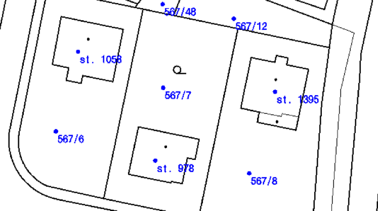
Since our interest is in the built-up structure, we restrict our attention to the built-up land plots only (built-up land plot = a building on it).

Building footprints in the U.S.A.

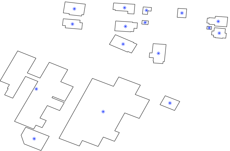
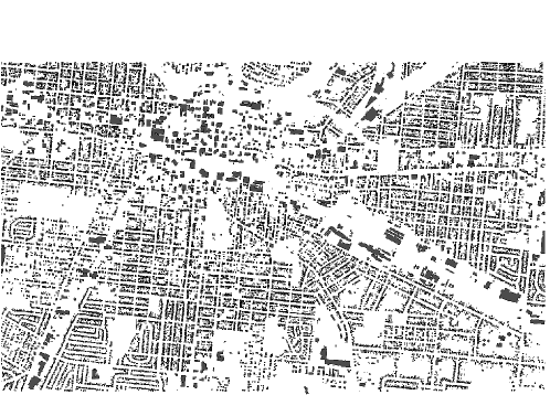
The second part of our data, the building footprints, are part of the GIS data in the ESRI Shapefile format available for few U.S.A. cities on the Internet (see section Resources for links). The building footprints are represented by polygons in the plane. Those polygons reflect the vertical projection of the overlaying buildings to the ground. Visualisation of a small part of the data is shown on the figure 2.

3.1. Representation

In order to analyse those different datasets we use two different but straightforward representations:

Point representation is given by the definition points (CR dataset) resp. centroids of polygons (U.S.A. dataset). For every city this gives a set of points $\{\boldsymbol{r}_{i},i\in I\}$. The order parameter that characterizes such point pattern is given by the singular point density $\rho(\boldsymbol{r})$ given by (5). The parameter variance $\sigma^{2}(R)$ means the variance of the number of points inside discs.

The estimation of $\sigma^{2}(R)$ for a given radius $R$ is done in the following way: Inside the investigated part of the city $A\subset\mathbbm{R}^{2}$ we uniformly and randomly choose centres $\boldsymbol{o}_{j}$ of $N$, $N>>1$ (usually $N=2000$) discs, so that every disc is a subset of $A$, $S(\boldsymbol{o}_{j},R)\equiv\boldsymbol{o}_{j}+S(R)\subset A$. For every disc $S(\boldsymbol{o}_{j},R)$ the number of inner points $N_{j}(R)$ is calculated,

(13) $$N_{j}(R)=\int_{S(\boldsymbol{o}_{j},R)}\rho(\boldsymbol{r})d\boldsymbol{r}.$$

The mean value is then estimated by

(14) $$\langle N(R)\rangle=\frac{1}{N}\sum_{j}N_{j}(R)$$

and the variance by

(15) $$\sigma^{2}(R)=\frac{1}{N-1}\sum_{j}\Big{(}N_{j}(R)-\langle N(R)\rangle\Big{)}^{2}.$$

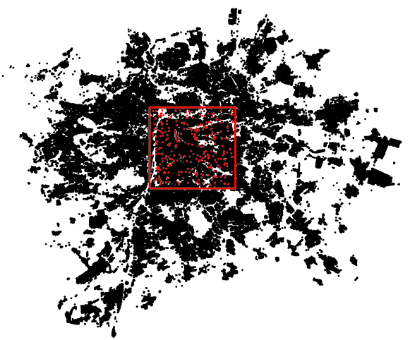
The example of a working area selection for Prague is shown in figure 3.

Figure 3. The point representation of Prague built-up land plots. The analyzed area is bounded by the red rectangle. The randomly positioned centres $\boldsymbol{o}_{j}$ of 200 discs are plotted as red points.

Set representation better reflects the existing structure of the built-up land. Let assume that we work only with the second dataset. Therefore the build-up land is given by non-intersecting polygons $\{p_{i}\subset\mathbbm{R}^{2},i\in I\}$. Such set can be represented as a subset of a plane given by boolean order parameter

(16) $$m(\boldsymbol{r})=\left\{\begin{array}[]{rll}1&\mathrm{building\ at\ }\boldsymbol{r},&(\exists i\in I,\boldsymbol{r}\in p_{i})\\ 0&\mathrm{othervise},&(\forall i\in I,\boldsymbol{r}\notin p_{i})\\ \end{array}\right.$$

The parameter variance $\sigma^{2}(R)$ can be estimated by use of (7).

If we want to deal with unknown shapes of the built-up parcels in the Czech case, the reasonable way is to approximate them by discs with the same area. Such approximation however cannot lead to the same (set) definition of the order parameter, because we generally cannot avoid the discs to overlap. This actually is not a problem and we can introduce the equivalent process of estimating $\sigma^{2}(R)$ that can be easily extended to the overlapping approximation.

Let us now suppose that our built-up parcels are given as a set $\{p_{i}\subset\mathbbm{R}^{2},i\in I\}$ but the non-intersecting property is generally not valid. This set is easily obtained for both datasets. In the Czech case $p_{i}$ is the circle of the same area $\lambda_{i}$ as the $i$-th land plot located at its definition point $\boldsymbol{r}_{i}$,

(17) $$p_{i}=\left\{\boldsymbol{r}\in\mathbbm{R}^{2}|\left|\boldsymbol{r}-\boldsymbol{r}_{i}\right|<\sqrt{\lambda_{i}/\pi}\right\}.$$

In the U.S.A. $p_{i}$ remains the polygon of the $i$-th building.

The estimation of $\sigma^{2}(R)$ for a given radius $R$ is then done as follows: Inside the studied part of the city $A\subset\mathbbm{R}^{2}$ we uniformly and randomly choose centres $\boldsymbol{o}_{j}$ of $N$, $N>>1$ discs, so that every disc is contained in $A$, $S(\boldsymbol{o}_{j},R)\equiv\boldsymbol{o}_{j}+S(R)\subset A$. For every disc $S(\boldsymbol{o}_{j},R)$ the built-up area $M_{j}(R)$ inside it is calculated by the relation

(18) $$M_{j}(R)=\sum_{i\in I}\lambda\left(p_{i}\cap S(\boldsymbol{o}_{j},R)\right),$$

where $\lambda(A)$ stands for the area of the set $A$. In other words, we accumulate the area of every intersection of the land plot $p_{i}$ with the given disc $S(\boldsymbol{o}_{j},R)$ over all land plots.

The process of calculating the area inside the disk $S(\boldsymbol{o}_{j},R)$ for polygons is depicted in figure 4.

Figure 4. The example of a built-up area calculation for a set representation of the U.S.A. dataset. The area $M_{j}(R)$ of polygons inside the disc $S(\boldsymbol{o}_{j},R)$ is marked as red.

The calculation of $M_{j}(R)$ for the polygons (U.S.A. dataset) is exact. On the other hand the disc approximation gives only an approximate result. The error is however not large and it is easy to show that the effective error is inversely proportional $R$

(19) $$\frac{\widehat{M_{j}(R)}-M_{j}(R)}{\widehat{M_{j}(R)}}\sim R^{-1},$$

with increasing $R$. Here $\widehat{M_{j}(R)}$ is the correct built-up area acreage inside the $j$-th disc. This is because for $R$ much larger than the typical parcel radius, deviations are produced only in the vicinity of the large disc boundary.

The mean value is estimated by

(20) $$\langle M(R)\rangle=\frac{1}{N}\sum_{j}M_{j}(R)$$

and the variance by

(21) $$\sigma^{2}(R)=\frac{1}{N-1}\sum_{j}\Big{(}M_{j}(R)-\langle M(R)\rangle\Big{)}^{2}.$$

The estimations for the both representations are based on the assumption of self-averaging property [20, 21]. It means that a sufficiently large sample is a good representative of the whole ensemble. In our case however, the size of the sample is limited by the size of the city centre. By the city centre we mean the area around the city core (central ’plateau’), where the built-up density is virtually constant [8]. This part of the city does not participate in a process of massive urbanization in contrary to the edges of the city. It thus represent a structure in a steady state (slowly varying). This does not exclude some local urbanization changes that are always presented. In order to speak about a virtually uniform density it is also necessary to omit certain locations like lakes or hilly places where it is impossible to construct a building from the analysis. Otherwise the fluctuations will increase.

4. Results

We analyzed the 6 largest cities in the Czech Republic and 6 cities in the U.S.A. In the centre of every city we calculated both the point number variance in discs (point representation) and the built-up area variance in discs (set representation) for different values of the disc radius $R$. The diameter of the city centre for a typical large Czech city is about 4 km. This size puts limitation on the maximal radius $R$ of discs in order to obtain reasonable statistics. Together with the fact that the power law dependence, if present, can be theoretically reached for $R\gg 1$, we decided to study the fluctuations inside the region $200\ \mathrm{m}\ \lesssim R\lesssim 1000\ \mathrm{m}$.

Figure 5. Dependencies of $\sigma^{2}(R)$ for the set representation on $\langle M(R)\rangle$ for different cities in the Czech republic.

Figure 6. Dependencies of $\sigma^{2}(R)$ for the set representation (polygon) on $\langle M(R)\rangle$ for different cities in the U.S.A.

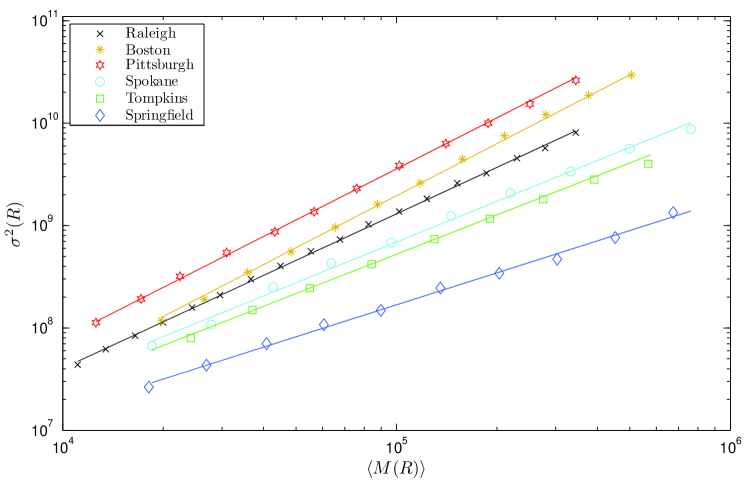
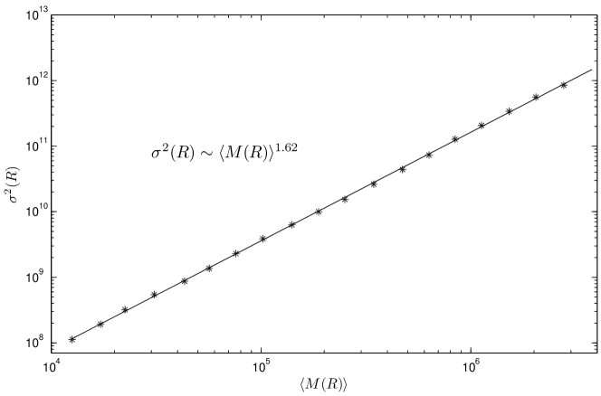
The obtained dependencies of $\sigma^{2}(R)$ on $\langle M(R)\rangle$ for the set representation are shown on figures 5 and 6. It is clearly visible that for the set representation the result follows power law (inside the analysed radius range). The same behaviour is valid also for the point representation. Thus in the studied range the fluctuations behave as

(22) $$\sigma^{2}(R)\propto\langle M(R)\rangle^{\alpha},\quad\alpha=2-\frac{\eta}{2}.$$

We determine the values of the exponent $\alpha$ by performing the linear regression on the logarithm relation

(23) $$\log(\sigma^{2}(R))=\alpha\log(\langle M(R)\rangle)+\beta.$$

The dependency of $\langle M(R)\rangle$ on $R$ resp. $\sigma^{2}(R)$ on $R$ follows the power law with exponent 2 resp. $2\alpha$ as predicted by the homogeneity assumption resp. the relation (12).

Table 1. Exponents $\alpha$ according to the power law dependence (22) of $\sigma^{2}(R)$ on $\langle M(R)\rangle$. In the 2-nd and 5-th column are values of the exponent for the point representation. The 3-rd and 6-th columns contain values for the set representation with circular approximation of the built-up units (for U.S.A. dataset - circles with the origin in the centroid and the same size as actual polygon). The 7-th column contains values for the set representation using the actual known polygonal shape of the building footprints.

City	Points	Area	City	Points	Area
		circle			circle	polygon
Praha	1.47	1.64	Raleigh	1.73	1.58	1.58
Plzeň	1.61	1.69	Pittsburgh	1.62	1.62	1.62
Liberec	1.54	1.65	Boston	1.69	1.68	1.69
Brno	1.40	1.65	Spokane	1.69	1.57	1.59
České Budějovice	1.50	1.58	Tompkins	1.75	1.57	1.59
Ostrava	1.54	1.62	Springfield	1.52	1.30	1.30

The summary of resulting exponents $\alpha$ for studied cities is given in the table 1. As follows from (11), $\alpha=1$ stands for the system that is outside of the critical region, e.g. randomly positioned particles. One can see that this is not the case for the built-up land pattern.

The values of the exponent for the built-up land pattern are for both representations much larger than 1. In the case of a point pattern the average value of the exponent is $\overline{\alpha}_{p}=1.60$. We can see a systematic difference between the Czech cities (lower values) and the American ones (larger values).

More interesting results arise for the set representation. There is not a clear systematic difference in this case between the Czech republic and the U.S.A. The average value of the exponent is $\overline{\alpha}_{a}=1.62$ with much lower fluctuations around this value. The only significant deviation in the power law coefficient is represented by the City of Springfield (Clark County). Such a result can be explained by its constrained lattice-like structure (see figure 7). Because the fluctuations are influenced by the local inhomogeneities of the pattern, the lattice-like structure produce a more homogeneous distribution (with lower fluctuations) of the built-up land than for the other more ”organic” cities [4]. Theoretically in the case of an exactly rigid structure with identical buildings placed at the vertices of a perfect lattice the fluctuations will increase and the coefficient $\alpha<1$. For further information on this so-called superhomogeneous distribution see [19].

Figure 7. The constrained structure of Springfield. The built-up land is plotted in its exact polygonal representation.

Comparing the values of the exponent $\alpha$ in the 6-th and 7-th column of the table 1 we can conclude that the approximation of an unknown parcel shape by a circle does not produce significant error.

Let us now make a short comment on the analysed range of $R$. In our analysis we used the interval $(200\ \mathrm{m},1000\ \mathrm{m})$. For some large cities in the U.S.A. we were eventually able to increase the upper bound to 3 km, because the analysed city centre area can be taken larger than for Czech cities that are much smaller. The power-law dependence remains unchanged in the extended range (see figure 8 for Pittsburgh in the set representation).

Figure 8. Fluctuation dependence in Pittsburgh for a set representation (polygons) in the region $R\in(200,3000)$ m. Straight line represents linear regression fit according to the logarithm relation (23).

Some further extension of the region can be also calculated but the assumption about the homogeneity (constant density) of the distribution is then obviously not valid since the density decreases with the increasing distance from the city centre. This influences the presented estimations of $\sigma^{2}(R)$ because the self-averaging cannot be applied. So even if the correlations may be evaluated on much larger distances, it is not proper to use this method outside of the theoretical homogeneous region.

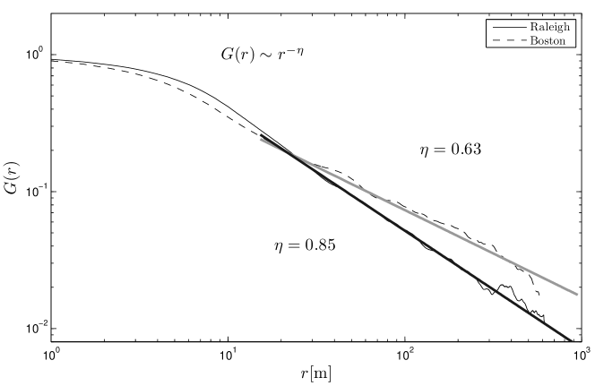
For the polygon representation of the built-up land in the U.S.A. it is also possible to estimate the correlation function directly. Results for Raleigh and Boston are shown in figure 9. The correlation function decay clearly follows a power law and the exponents are consistent with the values of $\alpha$ from table 1 and the relation (22). The same consistency holds for the rest of the studied cities.

Figure 9. The correlation function for Raleigh and Boston. Straight lines represent the linear regression fit of correlation function tails. Expected power-law tail coefficients $\eta$ calculated from the respective values of $\alpha$ in table 1 (according to (22)) are $\tilde{\eta}=0.84$ for Raleigh, resp. $\tilde{\eta}=0.62$ for Boston.

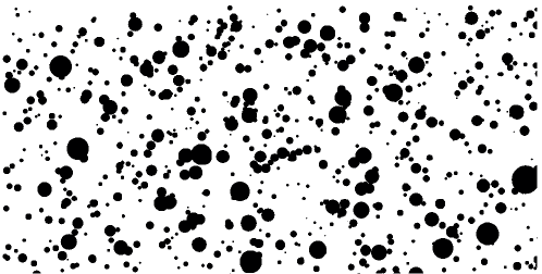
Finally we generated an artificial city by positioning the centres of the buildings randomly. Buildings were approximated by circles with a size distributed with the same distribution as for a real city. The part of this artificial city is shown in figure 10.

Figure 10. Part of a randomly generated city.

The correlation function for such pattern compared with the correlation function for Raleigh is shown in figure 11.

Figure 11. The correlation function for randomly generated pattern compared to the correlation function for Raleigh.

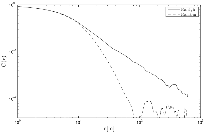
The fluctuation properties of such pattern are consistent with the predictions given by (11).

5. Conclusion

The study shows that dependence of fluctuations of the size of the build up area on its mean value follows a power law. Moreover the set representation of the plots seems to lead to more universal results. The values of the exponent $\alpha$ in the relation $\sigma^{2}(R)\sim\langle M(R)\rangle^{\alpha},$ for different cities (except of Springfield) are all very close to the value $\alpha=1.62$. The different results for Springfield can be explained by the strongly constrained lattice-like structure of that city.

We can conclude that the inner urban area structure is correlated with a long-ranged power-law dependence. The power-law exponent seems to be independent of the particular city. Such an observation is interesting and the possible connection between the urban area correlations and the correlations in critical systems may be useful for the development and verification of further urban models. The fact that the inner (quasi-stable) part of the city has certain city independent properties supports the hypothesis of the self-organized criticality in the urban systems [14]. However we are not able to study the process of the self-organization in details because our data do not reflect the dynamics of city growth, as we have only one time snapshot for each city.

Resources

The building footprints for U.S.A. cities were obtained from the following web sites:

• Boston - http://www.mass.gov/mgis/database.htm

• Raleigh - http://www.wakegov.com/gis/default.htm

• Pittsburgh - http://www.alleghenycounty.us/dcs/gis.aspx

• Spokane - http://www.spokanecity.org/services/gis/

• Tompkins - http://cugir.mannlib.cornell.edu/index.jsp

• Springfield (Clark County) - http://gis.clark.wa.gov/gishome/

References

- [1] Frank Schweitzer. Brownian Agents and Active Particles. Springer, first edition, 2003.
- [2] George Kingsley Zipf. Human Behavior and the Principle of Least Effort. Addison-Wesley, 1949.
- [3] Hernán D. Rozenfeld, Diego Rybski, Xavier Gabaix, and Hernán A. Makse. The area and population of cities: New insights from a different perspective on cities. NBER Working Papers 15409, National Bureau of Economic Research, Inc, October 2009.
- [4] Michael Batty and Paul Longley. Fractal Cities: A Geometry of Form and Function. Academic Press, first edition, 1994.
- [5] P. Frankhauser and R. Sadler. Fractal analysis of urban structures. Natural Structures - Principles, Strategies and Models in Architecture and Nature. Proc. Int. Symp. SFB 230, 4:57–65, 1992.
- [6] H. E. Stanley, L. A. N. Amaral, J. S. Andrade, S. V. Buldyrev, S. Havlin, H. A. Makse, C. K. Peng, B. Suki, and G. Viswanathan. Scale-invariant correlations in the biological and social sciences. Philosophical Magazine Part B, 77(5):1373–1388, 1998.
- [7] H. Eugene Stanley, José S. Andrade, Shlomo Havlin, Hernán A. Makse, and Béla Suki. Percolation phenomena: a broad-brush introduction with some recent applications to porous media, liquid water, and city growth. Physica A, 266(1-4):5– 16, 1999.
- [8] Marianne Guérois and Denise Pumain. Built-up encroachment and the urban field: a comparison of forty european cities. Environment and Planning A, 40:2186–2203, 2008.
- [9] Hernán A. Makse, Shlomo Havlin, and H. Eugene Stanley. Modelling urban growth patterns. Nature, 377:608–612, oct 1995.
- [10] Hernán A. Makse, José S. Andrade, Michael Batty, Shlomo Havlin, and H. Eugene Stanley. Modeling urban growth patterns with correlated percolation. Phys. Rev. E, 58(6):7054–7062, Dec 1998.
- [11] Hernán D. Rozenfeld, Diego Rybski, José Andrade, Michael Batty, H. Eugene Stanley, and Hernán A. Makse. Laws of population growth. PNAS, 105(48):18702–18707, 2008.
- [12] Diego Rybski, Sergey V. Buldyrev, Shlomo Havlin, Fredrik Liljeros, and Hernán A. Makse. Scaling laws of human interaction activity. PNAS, 106(31):12640–12645, 2009.
- [13] Per Bak, Chao Tang, and Kurt Wiesenfeld. Self-organized criticality. Phys. Rev. A, 38(1):364–374, Jul 1988.
- [14] Michael Batty and Yichun Xie. Self-organized criticality and urban development. Discrete Dynamics in Nature and Society, 3:109–124, 1999.
- [15] Igor Herbut. A Modern Approach to Critical Phenomena. Cambridge University Press, Cambridge, U.K., 2007.
- [16] Kerson Huang. Statistical Mechanics. John Wiley & Sons, 2nd edition, 1987.
- [17] L. D. Landau and E. M. Lifschitz. Statistical Physics. Pergamon Press, 3rd edition, 1980.
- [18] Zoltán Eisler, Imre Bartos, and János Kertész. Fluctuation scaling in complex systems: Taylor’s law and beyond. Advances in Physics, 57(1):89–142, 2008.
- [19] Andrea Gabrielli, Michael Joyce, and Francesco Sylos Labini. Glass-like universe: Real-space correlation properties of standard cosmological models. Phys. Rev. D, 65(8):083523, Apr 2002.
- [20] Didier Sornette. Critical Phenomena in Natural Sciences. Springer, 2000.
- [21] Amnon Aharony and A. Brooks Harris. Absence of self-averaging and universal fluctuations in random systems near critical points. Phys. Rev. Lett., 77(18):3700–3703, Oct 1996.