Bankruptcy Risk Model and Empirical Tests

Abstract

We analyze the size-dependence and temporal stability of firm bankruptcy risk in the US economy by applying Zipf scaling techniques. We focus on a single risk factor—the debt-to-asset ratio $R$—in order to study the stability of the Zipf distribution of $R$ over time. We find that the Zipf exponent increases during market crashes, implying that firms go bankrupt with larger values of $R$. Based on the Zipf analysis, we employ Bayes’ theorem and relate the conditional probability that a bankrupt firm has a ratio $R$ with the conditional probability of bankruptcy for a firm with a given $R$ value. For 2,737 bankrupt firms, we demonstrate size-dependence in assets change during the bankruptcy proceedings. Pre-petition firm assets and petition firm assets follow Zipf distributions but with different exponents, meaning that firms with smaller assets adjust their assets more than firms with larger assets during the bankruptcy process. We compare bankrupt firms with non-bankrupt firms by analyzing the assets and liabilities of two large subsets of the US economy: 2,545 Nasdaq members and 1,680 NYSE members. We find that both assets and liabilities follow a Pareto distribution. This is not a trivial consequence of the Zipf scaling relationship of firm size quantified by employees—while the market capitalization of Nasdaq stocks follows a Pareto distribution, this is not true for NYSE stocks. We propose a coupled Simon model that simultaneously evolves both assets and debt with the possibility of bankruptcy, and we also consider the possibility of firm mergers.

Complex systems are commonly coupled together and therefore should be considered and modeled as interdependent. It is important to study the conditions of interaction which may lead to mutual failure, the indicators of such failure, and the behavior of the indicators in times of crisis. As an indicator of economic failure, default risk is defined as the probability that a borrower cannot meet his or her financial obligations, i.e. cannot make principal and/or interest payments Duffie ; Lando . Accordingly, it is important to better understand default risk Duffie ; Lando ; Beaver66 ; Altman68 ; Altman77 ; Ohlson80 ; Scott ; Zmijewski84 ; Schary ; Dichev ; Shumway ; Beaver and its relation to firm growth Simon1 ; Ijiri ; Jovanovic1 ; Sutton1 ; Sutton2 ; pnas1 , and how they behave in times of crisis.

In describing both natural and social phenomena, size-dependent scaling is an essential technique for understanding the common relations between large and small scales. One reason for the importance of scaling relationships is that they capture salient, robust features of a system. Sala-i-Martin found by analyzing the scaling relation between GDP growth rates and initial GDP over the thirty-year period 1960–1990 that poor countries grow slower than rich countries martin96 . Size-dependent scaling of the standard deviations of firm growth rates and country growth rates are reported in Stanley3 and Lee . In finance, Fama and French demonstrated that market risk depends upon the firm size fama .

We find that book values of assets and debt of the U.S. companies that filed for bankruptcy in the past twenty years follow a Zipf scaling (power-law) distribution. The same is true for the values of assets and debt of non-bankrupt firms comprising the Nasdaq. We focus our attention on a single risk indicator, the debt-to-asset ratio $R$, in order to analyze stability of the scaling exponent or establish crossover regions. In order to capture Pareto and Zipf laws, the literature has typically focused on a single Simon model Simon1 ; Ijiri ; Sutton1 ; Sutton2 ; pnas1 describing a single dynamic system which does not interact with others. We model the growth of debt and asset values using two dependent (coupled) Simon models with two parameters only, bankruptcy rate and another parameter controlling debt-to-asset ratio. The Zipf law scaling predictions of the coupled Simon model are consistent with our empirical findings.

I Data Analyzed

Our dataset consists of medium-size and large U.S. companies that filed for bankruptcy protection in the period 1990–2009. We obtain our data from the URL www.BankruptcyData.com, one of the most comprehensive bankruptcy dataset currently available on the web. There is also a bankruptcy data set available at http://bdp.law.harvard.edu/fellows.cfm, but with smaller firms and no debt data. Our dataset includes data on 2,737 public and private firms. The book value of firm assets in the database ranges from 50 million to almost 700 billion USD.

• For each firm in our sample we know the pre-petition book value of firm assets $A_{a}$ and the effective date of bankruptcy. From the court petition documents we find the petition book value of firm assets $A_{b}$, as well as book value of total debt, $D_{b}$. As an example Lehman Brothers filled a petition on September 15, 2008, listing the debt $D_{b}$ and assets $A_{b}$ on May 31, 2008. Thus, $A_{b}$, $A_{a}$, and $D_{b}$ quantify the debtor’s condition before declaring bankruptcy. We are able to obtain $A_{b}$ and debt $D_{b}$ for 462 firms. Note that Refs. Altman77 , Ohlson80 , and Beaver studied 53, 105, and 585 bankrupt firms, respectively. There is often a substantial change in the debt and assets of a company in the time period preceding bankruptcy. Hence for each firm we calculate the debt-to-assets (leverage ratio)

  $$R\equiv D_{b}/A_{b},$$ (1)

  from the total debt $D_{b}$ and assets $A_{b}$ estimated simultaneously. Note that economics has a parallel treatment, known as Tobin’s Q theory of investment which also focuses on a single factor, Q Tobin .

  In the literature on ratio analysis Altman68 ; Ohlson80 ; Zmijewski84 , multiple financial ratios are used for predicting probability of default, such as the ratio of total liabilities to total assets. Adding more factors would likely improve the predictive power of the model, so we consider only one risk factor, namely the debt-to-assets ratio $R$ which captures the level of company indebtedness. We do this for two reasons: (a) to make a model as simple as possible, and (b) in order to simplify our study regarding whether market crashes and global recessions affect the scaling existing in bankruptcy data. In order to relate the probability of bankruptcy to $R$, we analyze the scaling relations that quantify the probability distribution of firms that entered into bankruptcy proceedings with particular values of $A_{b}$ and $R$. Our analysis includes very few number of young start-up firms, for which the age of the firm also factors into the probability of bankruptcy in addition to $R$. In 2009 we find that the average lifetime of the 215 bankrupt firms analyzed was $35.8\pm 33.9$ years, and the minimum lifetime was 3 years.

• We analyze market capitalization, assets and liabilities of 2,545 firms traded on the Nasdaq over the three-year period from 2006 to 2008. We also analyze assets and liabilities of 1,680 firms traded on the New York Stock Exchange (NYSE) in the period from 2007 to 2009. Also, we analyze market capitalization of NYSE members over the period 2002-2007.

II Quantitative Methods

Our analysis is closely related to the literature on firm size EL ; Axtell1 . Analyzing data from the U.S. Census Bureau, Ref. Axtell1 reported that firm sizes of the U.S. firms follow a Zipf law: the number of firms larger than size $s$ is $s^{-\zeta}$, where $\zeta\simeq 1$. The Zipf distribution is found for the distribution of city sizes Gabaix1 and the distribution of firm sizes Axtell1 ; Gabaix09 .

The cumulative distribution is a simple transformation of the Zipf rank-frequency relation, where the observations $x_{i}$ are ordered according to rank $r$ from largest ($r\equiv 1$) to smallest. For Pareto-distributed variables $s$ with cumulative distribution $P(s>x)\sim x^{-\zeta^{\prime}}$, the Zipf plot of size $s$ versus rank $r$ exhibits a power-law scaling regime with the scaling exponent $\zeta$, where

$$\zeta=1/\zeta^{\prime}.$$ (2)

III Results of Analysis

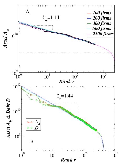
Figure 1: Zipf plot of U.S. bankrupted firm assets. (a) Zipf plot calculated for firms over the last 20 years between pre-petition total assets, $A_{a}$ versus rank. Deviation from the Zipf law is due to the fact that the data set includes mainly the firms with assets larger than 50 million dollars (dotted line). (b) Zipf plot of U.S. bankrupted firms of debt versus rank—462 firms in total—along with Zipf plot of book value asset and rank. The two plots practically overlap.

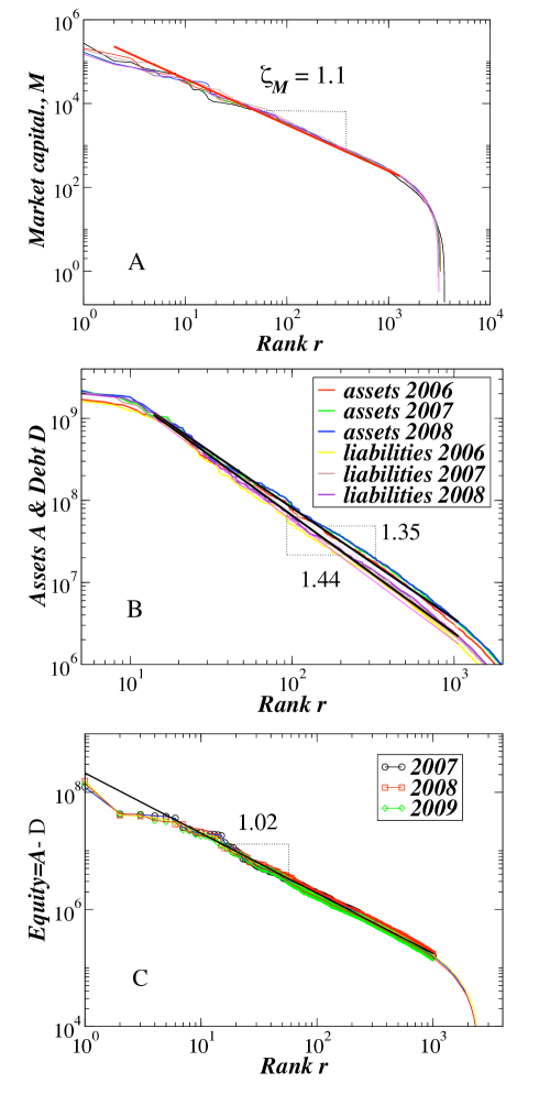
Figure 2: (a) Zipf plot of market capitalization $M$ versus rank $r$ for the Nasdaq members for each year of 6 years. We find practically the same Zipf law for the largest 1,000 companies as we find for the assets $A_{a}$ of bankrupted firms in Fig. 1(b). (b) For the Nasdaq firms both assets and liabilities follow a Zipf plot. (c) Book value of equity of stock traded at Nasdaq, defined as assets less liabilities, follows a Zipf law.

Figure 1(a) shows the Zipf plot for pre-petition book value of assets $A_{a}$. The data are approximately linear in a log-log plot with the exponent

$$\zeta_{{a}}=1.11\pm 0.01,$$ (3)

obtained using the OLS regression method. For the U.S. data on firm size (measured by the number of employees), Ref. Axtell1 reported the value $\zeta\approx 1$. Hence, prior to filing for bankruptcy protection, the book value of firm assets for companies that later underwent bankruptcy satisfies a scaling relation similar to that in Axtell1 . The firms with a rank larger than $\approx 500$ start to deviate from the Zipf law, a result of finite size effects as found in data on firm size Axtell1 .

It is known that the market equity of firms that are close to bankruptcy is typically discounted by traders Dichev ; Beaver . In order to study if those changes are size-dependent during the time of bankruptcy, we test whether there is a difference in scaling behavior between pre-petition and petition firm assets. Figure 1 B ranks the firm book value of assets $A_{b}$ and firm debt $D_{b}$. We find

$$\zeta_{{b}}=\zeta_{D}=1.44\pm 0.01.$$ (4)

Also, a Zipf law is found for the distribution of total liabilities of bankrupted firms in Japan Hideki ; Fujiwara .

We obtain that $\zeta_{b}>\zeta_{a}$, a discrepancy that could be of potential practical interest. To clarify this point, if $A_{b}$ is related to $A_{a}$ by a constant $A_{b}/A_{a}\equiv c$, we would observe $\zeta_{{a}}=\zeta_{{b}}$. However, we observe an increasing relation $A_{a}/A_{b}\propto r^{\zeta_{{b}}-\zeta_{{a}}}$ with rank $r$, meaning that bankrupt firms with smaller $A_{a}$ have larger relative adjustments than do bankrupt firms with larger $A_{b}$. By using a method proposed in Ref. GabaixJBES we obtain $\zeta_{b}=1.39$, close to the exponent we found in Eq. (4).

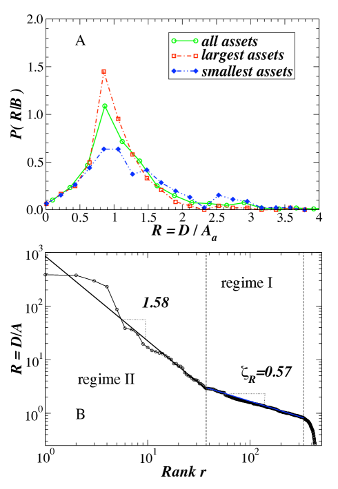
Figure 3: Bankruptcy risk based on petition book value asset $A_{b}$ and debt $D_{b}$. (a) We find the distribution of $R=D_{b}/A_{b}$ for the bankrupted firms. One may calculate the probability that a firm with a given ratio $R$ will go bankrupt when its ratio is $\leq R$. (b) For the ratio values $3>R>0.8$ (67% of all data), we show the Zipf plot that can be approximated by a Pareto distribution with $\zeta_{R}=0.57$. The same regime we fit with the power-law tail of pdf and obtain $0.79R^{-2.72}$ where the exponent $\zeta^{\prime}+1=2.73$ is in agreement (see Eq. (2)) with the Zipf exponent $\zeta=0.57$. For the largest ratio values $R>3$ (7% of all data), we find a crossover to a power-law regime with $\zeta_{R}=1.58$.

Our analysis of bankruptcy probability is, due to data limitation, based on book values. One may argue that a more relevant analysis would be based on market values of assets and liabilities. We now demonstrate that using market instead of book values may in fact lead to similar results. For this purpose, let us consider companies for which we have both market and book value data, namely stocks that comprise the Nasdaq. We begin by finding market capitalization of Nasdaq members for each year from 2002 to 2007. The data are available at www.bloomberg.com. Figure 2(a) shows the Zipf plot for market capitalization deflated to 2002 dollar values. We find that the market capitalization versus rank for the largest $\approx 1,000$ companies is well described by a Zipf law with exponent $\zeta_{M}=1.1\pm 0.02$, in agreement with Ref. Jovanovic3 .

In Fig. 2(b) we repeat the Zipf analysis using, this time, book values of both assets and debt for the same Nasdaq stocks. The scaling exponents we observe in Fig. 2(b) are larger than the exponent observed in Fig. 2(a). However, market capitalization is best compared with book value of equity $E\equiv A-D$, rather than assets $A$. In Fig. 2(c) we find that $E$ also exhibits Zipf scaling with exponent $\zeta_{E}=1.02\pm 0.01$, which is more similar to $\zeta_{M}$. Therefore, we find qualitatively similar scaling for the existing Nasdaq companies and for companies before they entered into bankruptcy proceedings.

The probability of bankruptcy $P(R)$ is a natural proxy for firm distress Dichev . Previous studies analyzed defaults of firms traded at NYSE, AMEX, and Nasdaq Dichev . In contrast, the majority of firms in our dataset are privately held companies. For bankrupt firms in Fig. 3(a) we show $P(R|B)$ for values of the debt-to-assets ratio $0<R<4$. We truncate data to avoid outliers as in Ref. Shumway . We find $P(R|B)$ is right-skewed with a maximum at $R\approx 1$, and $\langle R\rangle=1.4\pm 1.5$.

Previous studies find that bankruptcy risk of NYSE and AMEX stocks is negatively related to firm size Dichev . In order to test for firm-size dependence of bankruptcy risk for mainly private firms using BankruptcyData.com with $R$ as bankruptcy measure, we divide the $R$ values into two subsamples based on their value of $A_{b}$. In Fig. 3(a) we demonstrate qualitatively that $R$ is size-dependent. The pdfs for small $A_{b}$ and large $A_{b}$ are similar in that they both show peaks at $R\approx 1$. However, firms with smaller assets, as measured by $A_{b}$, have a larger probability of high debt-to-assets ratios $R$ than firms with large assets $A_{b}$.

In addition, we test for the size-dependence by performing the Mann-Whitney U-test, which quantifies the difference between the two populations based on the difference between the asset ranks of the two samples. (The null hypothesis is that the distributions are the same). Since the test statistics U-value $=-5.60$, we reject the null hypothesis thus confirming that $R$ depends on $A_{b}$ at the $p=0.05$ confidence level.

In Fig. 3(b) we analyze the Zipf scaling for large $R$. We find that the Zipf plot can be approximated by two power-law regimes. For $\approx 300$ firms with $0.8<R<3$ (regime I), we find a power-law regime with $\zeta_{R}=0.57\pm 0.02$. Hence, according to Eq. (2) we conclude that the cumulative distribution of dangerously high $R$ values of bankrupt firms decreases faster with $\zeta^{\prime}\approx 1.72$ for large $R$ than the distribution of firm size Axtell1 and firm assets with $\zeta^{\prime}\approx 1$ (see Fig. 1). For $R>3$ (7% of all data including predominantly financial firms), we find that the Zipf plot exhibits a significant crossover behavior to a power-law regime with $\zeta\approx 1.58$.

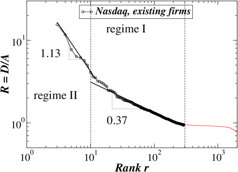
Figure 4: Zipf plot of debt-to-assets ratio $R$ and rank $r$ for the existing firms of the Nasdaq members over the last 3 years. For the $\approx 300$ ratio values smaller than 3.5 and larger than 0.95 the Zipf plot has exponent 0.37. The same regime we fit with the power-law tail of pdf and obtain $1.54R^{-3.6}$ where the exponent $\zeta^{\prime}=3.6$ agrees [see Eq. (2)] with the Zipf exponent $\zeta=0.37$.

The conditional probability $P(B|R)$ that an existing firm with debt-to-assets ratio $R$ will file for bankruptcy protection may be of significance to rating agencies, creditors, and investors. According to Bayes theorem, $P(B|R)$ depends on $P(R|B)$ (see Fig. 3), $P(B)$, the probability of bankruptcy for existing firms, and $P(R)$ where as a proxy for the existing companies we use companies constituting the Nasdaq in the 3-year period between 2007–2009. For this time period we obtain book value of each firm’s assets and liabilities (the latter serving as a proxy for total debt). As a result we obtain 7,635 $R$ values with median value 0.48. For existing Nasdaq members, Fig. 4 shows that the Zipf plot can be approximated by two power-law regimes, where regime I with $3.5>R>0.9$ yields $\zeta_{e}=0.37\pm 0.01$. Note that regime I is similar to the one we find in Fig. 3(b) for bankruptcy data. $P(B)$ may substantially change during economic crises. Interestingly, Ref. DebtEPL analyzes the debt-to-GDP (gross domestic product) ratio for countries, in analogy to the debt-to-assets ratio for existing firms, and calculates a Zipf scaling exponent that is approximately the same as the scaling exponent calculated here for existing Nasdaq firms.

We estimate the scaling of $P(B|R)$ using Bayes’ theorem,

$$P(B|R) = \frac{P(R|B)P(B)}{P(R)}\approx 0.51~{}P(B)R^{1/\zeta_{e}-1/\zeta_{R}}$$ (5)

$$\approx 0.51~{}P(B)~{}R^{0.95}$$

where we approximate $P(R|B)$ and $P(R)$ with power laws—$P(R|B)\sim R^{-(1/\zeta_{R}+1)}\Delta R$ and $P(R)\sim R^{-(1/\zeta_{e}+1)}\Delta R$. The value of the relevant exponents calculated for regime I are: $\zeta_{e}\approx 0.37$ (see Fig. 4) and $\zeta_{R}=0.57$ [see Fig. 3(b)], where $\zeta_{R}>\zeta_{e}$ implies that $P(B|R)$ increases with firm indebtedness quantified by $R$. The pre-factor 0.51 calculated for the regime I we estimate from the corresponding intercepts in pdfs [see Figs. 3(b) and 4]. In Fig. 4 we find a pronounced crossover in the Zipf plot for very large values of the $R$ ratio.

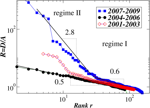
Figure 5: Zipf plot of debt-to-assets ratio $R$ versus rank $r$ for the bankrupt firms for the three different 3-year subperiods. During the last three years characterized by recession the Zipf plot exhibits a crossover behavior. A smaller crossover in the Zipf plot also exists for the period 2001–2003 characterized by the dot-com bubble burst.

In order to test whether market crash and global recession have significant effects on the scaling we find in the bankruptcy data, in Fig. 5 we analyze the Zipf scaling of the large $R$ values for three different 3-year periods. For the period 2004–2006 we find a stable Zipf plot characterized by an exponent $\zeta_{R}=0.50\pm 0.01$ close to the value we found in Fig. 3(b) for all years analyzed. For the period 2001–2003 characterized by the dot-com bubble burst, we find a less pronounced crossover in the Zipf plot between regime I with exponent $\zeta_{R}=0.58\pm 0.01$ and regime II. For the period 2007–2009 we find that the Zipf plot exhibits a significant crossover behavior between regime I and regime II.

Figure 5 demonstrates the existence of a relatively stable scaling exponent (between 0.5 and 0.6) in regime I over the 9-year period 2001-2009. However, in times of economic crisis, e.g., the period 2007–2009, the exponent in regime I increases, implying that firms go bankrupt with larger values of $R$. According to Eq. (5), in times of crisis $(\zeta_{R}\approx 0.6)$ $P(B|R)\propto R^{1/\zeta_{e}-1/\zeta_{R}}~{}\propto R^{1}$ shifts upward compared to times of relative stability $(\zeta_{R}\approx 0.5)$ when $P(B|R)~{}\propto R^{0.7}$. A crossover in scaling exponents may be useful for understanding asset bubbles.

IV A Model

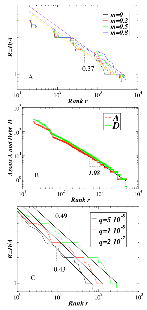
Figure 6: Model results. (a) Zipf plot of debt-to-assets ratio $R$ versus rank $r$ for the firms generated by the model (compare with Fig. 4) when bankruptcy is not included. In order to understand plateaus in the figure, note that both assets and debt in the model exhibit integer values. (b) For each asset and debt the Zipf plot displays a power law $R\sim r^{-\zeta}$. (c) Zipf plot of $R$ versus rank as a function of bankruptcy rate parameter $q$. With decreasing $q$ the slope increases slightly.

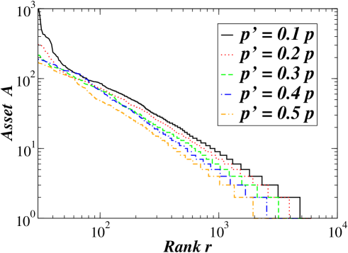
Figure 7: Scale-free persistence in the Simon model with mergers. Zipf plot of value $A_{j}(t)$—the value of assets of the firm $j$—versus rank $r$ for the Simon model with a merger parameter $p^{\prime}$ representing the probability that a pair of firms will merge. With increasing $p^{\prime}$, $\zeta$ slowly increases.

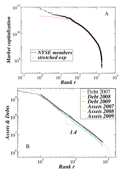
Figure 8: Zipf plot of (a) market capitalization $M$ versus rank $r$ and (b) assets and debt versus rank $r$ for the NYSE members for year 2007. The curve in (a) follows a stretched exponential $exp(-r^{\beta}/\tau)$ with $\beta=0.5$ and $\tau=45$.

Our results complement both the literature on default risk as well as the literature on firm growth. According to a study of U.S. firm dynamics, over 65% of the 500 largest U.S. firms in 1982 no longer existed as independent entities by 1996 Blair1 . To explain how firms develop, expand and then cease to exist, Jovanovic proposed a theory of selection where the key is firm efficiency; efficient firms grow and survive and the inefficient decline and, eventually, fail Jovanovic1 . Many models have been proposed to model default risk Duffie ; Lando ; Merton74 ; Black76 ; Long95 ; Hull95 . One strain of that literature Merton74 develops structural models of credit risk. In these models, risky debt is modeled within an option-pricing framework where an underlying asset is the value of company assets. Bankruptcy occurs endogenously when the value of company assets is insufficient to cover obligations. In contrast, in reduced form models Lando default is modeled exogenously.

In order to reproduce the Zipf law that holds for bankrupt firms, we propose a coupled Simon model, an extension of the Simon model used in the theory of firm growth Simon1 ; Ijiri ; Sutton1 ; Sutton2 ; pnas1 . Here we couple the evolution of both asset growth and debt growth through debt acquisition which depends on a firms assets, and further impose a bankruptcy condition on a firm’s assets and debt values at any given time.

Simon rule for assets. The economy begins with one firm at the initial time $t\equiv 1$. At each step a new firm with initial assets $A\equiv 1$ is added to the economy. With a probability $p$, a new firm $i$ is added to the economy as an individual entity at time $t_{i}$. With probability $1-p$, the new firm $i$ is taken over by another firm. The probability that firm $i$ is taken over by an existing firm $j$ is proportional to $A_{j}(t)$, the number of units in firm $j$ is equal to $(1-p)A_{j}(t)/\Sigma_{k}A_{k}(t)$. Hence, a larger firm is more likely to acquire a firm than a smaller firm. In this expression, the index $k$ runs over all of the existing firms at time $t$. We use the value $A_{j}(t)$ to be the proxy for the value of assets of the firm $j$. Simon found a stationary solution exhibiting power-law scaling, $P(s>x)\propto s^{-\zeta^{\prime}}$, with exponent $\zeta^{\prime}=1/(1-p)$. For an estimate of $p$ one can investigate venture data to see how venture capitalists dispose of their companies. Even though data suggest $p=0.5$ (see Jovanovic4 ), we use a much smaller value $p=0.01$ in oder to reproduce Zipf plot in Eq. (4).

Simon rule for debt. When a new firm $i$ is created at time $t_{i}$, it is assigned debt $D_{i}(t_{i})=m$, where $0<m<1$. For simplicity we use a single $m$ value for all firms. If an existing firm $j$ acquires the new asset $A_{i}\equiv 1$, then $A_{j}(t)-A_{j}(t-1)=1$, and debt $D_{j}(t)-D_{j}(t-1)=m$. Hence, a firm with assets $A_{j}(t)=N$ has debt $D_{j}(t)=mN$, implying that the debt-to-assets ratio $R=m$ is the same for all firms.

In order to introduce variation in $R$ ratios across firms, we assume that at each time $t_{i}$, a new debt is created in the economy for some company $j$, so that $D_{j}(t_{i})-D_{j}(t_{i}-1)=1$. Hence, for each time step, there is a new firm receiving debt $D_{i}=m$ in addition to firm $j$ receiving one unit of debt, where generally $i\neq j$. The newly created units of debt are acquired with probability proportional to $A_{j}(t)$. Hence, the Simon laws controlling the growth of debt $D_{j}(t)$ and the growth of assets $A_{j}(t)$ are coupled. In our model, richer firms become more indebted, but also acquire new firms with larger probability.

In Fig. 6(a) we perform the numerical simulation of the model by generating 500,000 Monte-Carlo time steps. We calculate the Zipf distribution of the debt-to-assets ratio $R$ for different choices of $m$. Even though debt and hence $R$ increases with $m$, the slope of the Zipf plot for $R$ versus rank practically does not depend on the value of $m$. Unless stated otherwise, in other simulations we set $m=0.5$.

Following Barabasi99 , we consider the continuous-time version of our discrete-time model. In this case $D_{j}(t)$ and $A_{j}(t)$ are continuous real-valued functions of time. Further, we assume that the rate at which $D_{j}(t)$ changes in time is proportional to the assets size $A_{j}(t)$. Hence, following this assumption, $D_{j}(t)=(1+m)A_{j}(t)$ because of the acquisition of additional debt. Therefore, since $A_{j}(t)=t/t_{j}$ Barabasi99 , then $D_{j}(t)=(1+m)t/t_{j}$. The cumulative probability that a firm has debt size $D_{j}(t)$ smaller than $D$ is, therefore, $P(D_{j}(t)<D)=P(t_{j}>(1+m)t/D)$. In the Simon model we add new firms at equal time intervals. Thus, each value $t_{i}$ is realized with a constant probability $P(t_{j})=1/t$. It follows that

$$P(t_{j}>(1+m)t/D)=1-(1+m)t/Dt=1-(1+m)/D.$$ (6)

Since the parameter $t$ cancels out, the same expression we obtain when $t$ goes to infinity. This is the Zipf law for debt in the case when there is no possibility of bankruptcy [see Eq. (3)].

Firm bankruptcy. Up to now, debt has been modeled as riskless. We now introduce bankruptcy into the coupled Simon model. We assume that for each firm there is a likelihood of bankruptcy, which depends on the volatile firm asset value Merton74 . In order to be consistent with our empirical findings, we assume that the firm $j$ that was created at time $t_{j}$ files for bankruptcy with probability $q~{}R^{0.95}$ [see Eq. (6)], where $q$ is the bankruptcy rate parameter, related to $P(B)$ in Eq. (6). In the hazard model, the hazard rate is the probability of bankruptcy as of time t, conditional upon having survived until time $t$ Shumway . In our model, once firm $j$ files for bankruptcy, part of its debt is lost (restructured) and the firm starts anew with debt equal to $D_{j}=mA_{j}$. We do not assume a merger or a liquidation and a firm’s probability of failure does not depend on its age Shumway . Besides bankruptcy, a firm may leave an industry through merger and voluntary liquidation Schary .

Next we perform 500,000 Monte-Carlo time steps for the model with the possibility of bankruptcy. Fig. 6(b) presents Zipf distribution for firm asset and debt values for all of the existing firms. Each of these distributions is in agreement with the Zipf law and Eq. (6). In Fig. 6(c), for the subset of bankrupt companies, we show the Zipf distribution for $R$ using three different values of the bankruptcy rate $q$. Note that $q$ is supposed to be small. Namely, with $q=10^{-7}$ and with 500,000 time steps representing one year, $500,000~{}q$ represents a probability per year that a company files for bankruptcy during a period of one year, $\approx 0.05$ in our case. This should be compared with the average default rate, $\approx 0.04$, calculated in the period 1985–2007 Altman07 . We see that model predictions approximately correspond to the empirical findings.

Our model can be extended in different ways including mergers between firms. First, while the Simon model assumes that at each time increment a new unit is added, we can assume that the number of new units grows as a power-law $t^{\theta}$ Dorogovtsev . By using a continuous-time version of a discrete-time model we obtain $P(D_{j}(t)<D)=P(t_{j}>(1+m)t/D)=1-(\frac{1+m}{D})^{1+\theta}$, where we use $P(t_{i}>t_{0})=\int_{t_{0}}^{t}dtt^{\theta}/\int_{0}^{t}dtt^{\theta}$. Second, Jovanovic and Rousseau Jovanovic4 found that mergers contribute more to firm growth than when a firm takes over a small new entrant. In order to incorporate mergers into the Simon model, we assume that at each time $t$, a single merger between a pair of firms occurs with probability $p^{\prime}$, where two firms are randomly chosen. Reference Andrade reported that in more than two thirds of all mergers since 1973, the Tobin $Q$ value of the acquisition firm exceeded the Tobin $Q$ value of the target firm, where $Q$ is Tobin ’s ratio similarly defined as $D$ ratio in Eq. (1). To this end, we assume that if $A_{j}>A_{i}$ when a merger occurs $A_{j}=A_{j}+A_{i}$ and $A_{i}=0$. Thus, the more-rich firm $j$ buys the less-rich firm $i$ resulting in the elimination of firm $i$ as an individual entity. In Fig. 7 we show that the inclusion of mergers does not change the scale free nature of the Simon model. In these simulations we use a varying merger probability $p^{\prime}$, and $p=0.01$ with 1,000,000 time steps. With increasing $p^{\prime}$, the Zipf exponent $\zeta$ slowly decreases. Note that with 1,000,000 time steps if $p^{\prime}=0.5p$, and with $p=0.01$, then approximately 5,000 mergers occur.

V Discussion and summary

We demonstrate that Zipf scaling techniques may be useful in analyzing bankruptcy risk. We find that book values of pre-petition and petition company assets systematically differ from each other and that the difference depends upon company size. Also, the debt-to-assets ratio $R$ for firms that filed for bankruptcy has a probability distribution that depends upon the firm size. In analyzing existing (non-bankrupt) companies we use as a proxy stocks traded at Nasdaq. We demonstrate that market capitalization as well as book value of assets, liabilities and equity for the stocks traded at Nasdaq exhibit Pareto scaling properties. This is not a trivial consequence of the scaling relationship of firm size Axtell1 since for companies traded at NYSE we do not find similar power-law scaling for market capitalization [see Fig. 8(a)] and book value of equity. However, the book value of assets and liabilities for NYSE stocks follows a Pareto law with exponents that are slightly larger than those we find for Nasdaq stocks [see Fig. 8(b)]. Our results reveal a discrepancy in scaling of market capitalization and book value of equity obtained from different exchange markets (e.g., Nasdaq and NYSE).

Using our scaling results, we derive a simple expression for the conditional bankruptcy probability given $R$. Importantly, we find that scaling properties for large $R$ values change during the periods of significant market turbulence such as the dot.com bubble crash (2001–2003) and the current global crisis where scaling exhibits significant cross-over properties. Change of scaling exponents may, therefore, be of significance understanding the asset bubbles.

In order to reproduce our empirical results we model growth of risky debt and asset values by means of two dependent (coupled) Simon models. Predictions of the coupled Simon model are consistent with our empirical findings.

References

- (1) Duffie D, Singleton K (2003) Credit Risk. Princeton University Press.
- (2) Lando D (2004) Credit Risk Modeling. Princeton University Press.
- (3) Beaver W (1966) Financial ratios as Predictors of Failure Journal of Accounting Research 4:71–111.
- (4) Altman E I (1968) Financial ratios, discriminant analysis and the prediction of corporate bankruptcy. J. Finance 23:589–609.
- (5) Altman E I, Haldeman R, and Narayanan P (1977) ZETA Analysis: A new model to identify bankruptcy Risk of Corporation. J. of Banking and Finance 1:29-54.
- (6) Ohlson J A (1980) Financial ratios and the probabilistic prediction of bankruptcy Journal of Accounting Research 18:109–31.
- (7) Scott J (1981) The probability of bankruptcy: A comparison of empirical predictions and theoretical models Journal of Banking & Finance 5:317-344.
- (8) Zmijewski M E (1984) Methodological issues related to the estimation of financial distress prediction models Journal of Accounting Research 22:59-82.
- (9) Schary M A (1991) The Probability of Exit. The Rand Journal of Economics 22:339-53.
- (10) Dichev I D (1998) Is the risk of bankruptcy a systematic risk? Journal of Finance 53:1131-1147.
- (11) Shumway T (2001) Forecasting Bankruptcy More Accurately: A Simple Hazard Model The Journal of Business 74:101-124.
- (12) Beaver W H, McNichols MF, Rhie JW (2005) Have Financial Statements Become less informative? Evidence from the ability of financial ratios to predict bankruptcy. Review of Accounting Studies 10: 93-122.
- (13) Simon HA (1955) On a class of skew distribution functions. Biometrika 42:425–440.
- (14) Ijiri Y, Simon H (1977) Skew distributions and the sizes of business firms. New York: North-Holland.
- (15) Jovanovic B (1982) Selection and the evolution of industry. Econometrica 50: 649–670.
- (16) Sutton J, Gibrat’s legacy (1989) Journal of Economic Literature 35:40–59.
- (17) Sutton J (1995) The size distribution of businesses, Part I: A benchmark case. LSE STICERD Research Paper No. EI09.
- (18) Fu D, et al. (2005) The Growth of Business Firms: Theoretical Framework and Empirical Evidence. Proc. Natl. Acad. Sci. USA 102:18801-18806.
- (19) Sala-i-Martin, X (1995) The classical approach to convergence analysis. The Economic Journal 106:1019–1036.
- (20) Stanley MHR, et al. (1996) Scaling behavior in the growth of companies. Nature 379:804–806.
- (21) Lee, Y. et al. (1998) Universal features in the growth dynamics of complex organizations. Phys. Rev. Lett. 81:3275–3278.
- (22) Fama EF, French KR (1993) Common risk factors in the returns on stocks and bonds. Journal of Financial Economics 33:3–56.
- (23) Tobin J (1969) A general equilibrium approach to monetary theory. J. of Money Credit and Banking 1:15–29.
- (24) Stanley MHR, et al. (1995) Zipf plots and the size distribution of firms. Economics Lett. 49:453–457.
- (25) Axtell RL (2001) Zipf distribution of U.S. firm sizes. Science 293:1818–1820.
- (26) Petersen AM, Podobnik B, Horvatic D, Stanley HE (2010) Scale-invariant properties of public-debt growth. Europhys. Lett. 90: 38006.
- (27) Gabaix X (1999) Zipf’s Law for cities: An explanation. Quarterly Journal of Economics 114:739–767.
- (28) Gabaix X (2009) Power laws in Economics and Finance Annu. Rev. Econ. 1:255–593.
- (29) Aoyama H, et al. (2000) Pareto’s law for the income of individuals and debt of bankrupt companies. Fractals 8:293-300.
- (30) Fujiwara Y (2004) Zipf law in firms bankruptcy. Physica A 337: 219-230.
- (31) Gabaix, X. & Ibragimov, R. Rank-1/2: A simple way to improve the OLS estimation of tail exponents. Journal of Business Economics and Statistics (in press).
- (32) Barbarino A, Jovanovic B (2007) Shakeouts And Market Crashes. International Economic Review 48:385–420.
- (33) Blair MM, Kruse DL, Blasi JR (1998) Is employee ownership an unstable form? Or a stabilizing force? Working paper. Brookings Institution: Washington, D.C.
- (34) Merton RC (1974) On the pricing of corporate debt: The risk structure of interest rates. J. Finance 29: 449–470.
- (35) Black F, Cox JC (1976) On the pricing of corporate debt: the risk structure of interest rates. J. Finance 31:351–367.
- (36) Longstaff FA, Schwartz ES (1995) A Simple Approach to Valuing Risky Fixed and Floating Rate Debt. J. Finance 50:789–819.
- (37) Hull J, White A (1995) The impact of default risk on the prices of options and other derivative securities. J. Banking and Finance 19:299–322.
- (38) Dorogovtsev S N, Mendes J F F, Samukhin A N (2000) Structure of Growing Networks with Preferential Linking Phys. Rev. Lett. 85:4633–4636.
- (39) Jovanovic B, Rousseau P. L (2001) Why Wait? A Century of Life before IPO American Economic Association 91: 336–341.
- (40) Andrade G, Mitchell M, Stafford E (2001) New evidence and perspective on mergers Journal of Economic Perspectives 15: 103–120.
- (41) Barabási AL (1999) Emergence of scaling in random networks. Science 286:509–512.
- (42) Altman E I, Karlin B J (2008) Report on Defaults and Returns in the High-Yield Bond Market: The Year 2007 in Review and Outlook New York University Salomon Center.