Level Crossing Analysis of Cosmic Microwave Background Radiation:
A method for detecting cosmic strings
Abstract
In this paper we study the footprint of cosmic string as the topological defects in the very early universe on the cosmic microwave background radiation. We develop the method of level crossing analysis in the context of the well-known Kaiser-Stebbins phenomenon for exploring the signature of cosmic strings. We simulate a Gaussian map by using the best fit parameter given by WMAP-7 and then superimpose cosmic strings effects on it as an incoherent and active fluctuations. In order to investigate the capability of our method to detect the cosmic strings for the various values of tension, , a simulated pure Gaussian map is compared with that of including cosmic strings. Based on the level crossing analysis, the superimposed cosmic string with in the simulated map without instrumental noise and the resolution could be detected. In the presence of anticipated instrumental noise the lower bound increases just up to .
I Introduction
One of the most interesting predictions of quantum field theory in the domain of cosmology is the possibility of transition between different vacuum states during the expansion of the universe. Depending upon the topology of these states, a series of stable topological defects such as domain walls, monopoles and cosmic strings can be formed. Regarding the formation of strings, they may have self-interactions causing the formation of closed loops according to the so-called inter-commutation neil07 ; neil10 ; matt09 ; hind94 ; sak06 ; vak84 ; vil85 ; vilinkin00 ; shell87 ; maxim99 . In principle, string loops start to oscillate and emit stochastic gravitational waves which results in their annihilation, allen96 while the infinite straight strings survive up to now. Although, in some models of inflation such as false vacuum dominated inflation (in the context of hybrid inflation theories), topological defects are formed at the end of inflation era cope94 , but the true focus on the issue of cosmic strings was in the recent years, mainly because new models of inflation derived from the superstring theory, result in acceptable possibility for the production of cosmic strings sar02 ; tye06 ; kibb04 ; cop03 . This is based on the consideration of cosmic string networks consisting of infinite strings, loops, and junctions of two or more strings which will definitely have effects such as lensing, CMB polarization, and of course CMB anisotropies. Astrophysical evidence of cosmic string strongly depends on the two following parameters, namely: dimensionless string tension ( is the Newton’s constant and stands for energy scale when the strings are created) and inter-commuting probability, . The quantity shows the mass per unit length of cosmic string. The energy density of cosmic string is associated with the scale of phase transition and symmetry breaking in which cosmic strings are produced. Generally the formation of cosmic strings could occur at very extended ranges of energy scale, e.g. the Grand Unified Theory (GUT) scale with GeV corresponding to , consequently there is a wide range of s has been supposed vilinkin00 ; firouz05 . It must be noted that the footprints of strings, such as anisotropies in CMB are directly affected by their tension. So determining the bounds for the tension, directly means limiting the fundamental theory on the basis of which cosmic strings are produced. To this end, observing the cosmic string footprints by using various approaches can be interpreted as a kind of observational evidence for the low energy limit of the superstring theory and would provide the most direct test of string theory and could rule out or constrain on particle physics models.
From theoretical and observational perspectives, there are a dozen constrains on the cosmic string’s parameters. Recent analysis by using pulsar timing and photometry based on gravitational microlensing put a constraint for tension in the range jent06 ; psh09 ; psh10 ; dam05 ; rich10 ; okn99 ; khlop89 ; khlop86 ; khlop82 . Using COSMOS survey, there is for cosmic string reported in smoot10 . The signature of cosmic string wakes has also been explained in Ref. branddd10 . Another robust constraint on the cosmic string’s free parameters comes from the temperature fluctuations at the last scattering surface. More recent full analysis and prediction for incoming satellite based surveys can be found in neil07 ; neil10 ; reg09 ; mark09 . Temperature fluctuations contain the accumulation of anisotropies induced by cosmic strings and can be divided into two categories: 1) anisotropies created by the so-called Kaiser-Stebbins effect and those related to pre-recombination processes and 2) the stochastic background of gravitational waves produced by decaying of string loops kaiser84 ; spergel08 . Calculation of temperature angular power spectrum puts the upper bounds spergel08 ; pre93b ; bevis05 ; wyman05 ; wyman06 ; bevis07 ; fra05 ; kaiser84 and at confidence interval for Abelian-Higgs case rich10 . Nambu-Goto numerical simulation for network of cosmic string has been used by A. A. Fraisse et al. spergel08 . For detecting the anisotropies induced by mentioned strings, temperature gradient magnitude operator has been applied in this paper. Ligo and Virgo collaborations recently have reported the newly lower and upper bounds as on the stochastic gravitational waves produced by cosmic strings ligo09 . The skewness in CMB fluctuations and its dependency on inter-commuting probability has been investigated in daisu10 . Based on B-mode polarization of cosmic microwave background new constraint on has been reported in Ref. zhe10 .
Direct implication based on the explicit recognition of discontinuity in the fluctuation of cosmic microwave background radiation is a unique signature of straight cosmic string , namely the Kaiser-Stebbins effect kaiser84 . In this part, there are also some upper bounds as well as lower bounds for distinguishing cosmic strings. Another method is the so-called Wavelet domain Bayesian denoising which has recently been used by D. K. Hammond et al. hammond09 . Since the cosmic string is characterized by a localized edge like discontinuity, they used a Steerable Pyramid wavelet transform to discriminate straight edge from other features. Transformation has been done with 6 orientations and 4 spatial scales. According to their results, the signature of cosmic strings in the CMB map without noise can be identified for tensions in the range while for a noisy map the lower bound increases more than one order of magnitude hammond09 . For completing this topic, reader can also refer to Refs. barr01 ; barr06 . The detectability threshold for cosmic string signal in the presence of anticipated noise such as extra-Galactic and Galactic foregrounds has been studied in jeong10 . A series of papers published by Brandenberger and his collaborators have been devoted to the ability of so-called Canny algorithm to detect the cosmic string and super strings according to Kaiser-Stebbins effect brand081 ; brand080 ; brand09 . They have concluded the lower bound of . Actually in the Canny method, the sharp and strength edges are picked up by means of the magnitude of the contrast from one side of produced edge to the other one brand081 . Non-gaussianity due to cosmic strings in addition to other events such as kinetic Sunyaev-Zel’dovich effect have been examined in stark03 by multi-scale methods (also see chi10 for more discussions). They have argued that to find a significant results not only one should use robust methods but also a combination of powerful methods is necessary.
Another most interesting method which is potentially able to discriminate map with and without cosmic strings as well as other topological defects is the so-called peak-peak correlation function peac85 ; bardeen86 ; hevan99 ; hevan01 . In this method, two-point correlation function of the local maxima (or minima) of temperature fluctuations on the CMB map at a typical peak threshold is determined. A. F. Heavens et al. have demonstrated that this correlation function for a simulated CMB map accompanying cosmic string grows up significantly at around arcminutes, relative to the pure Gaussian map. As they claimed, this procedure has no adjustable parameter, consequently it can be powerful for test of Gaussianity hypothesis as well as tracking the footprint of other mechanism for producing initial fluctuations in the upcoming high resolution observations. Although, they didn’t show the efficiency of this method for various values of which is the main purpose of this paper, but it is interesting reapply the same idea based on hotspots (or coldspots) framework. In our method not only we investigate all features of fluctuations instead of local extrema used in the peak-peak correlation function, but also the moments of relevant quantity are used (see section II for more details).
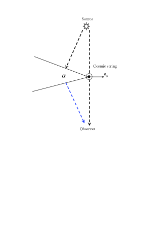
In this study we are relying on a newly demonstrated method to put a lower limit on the tension of straight cosmic strings in the high resolution of CMB map for which we can discriminate their signatures. As the effect of cosmic strings, we concentrate on the discontinuities and fluctuations in the CMB map arising from the Kaiser-Stebbins effect which is a part of integrated Sachs-Wolfe effect and can produce observational consequences on the anisotropies in the CMB map. This feature is based on the gravitational lensing which was a well-established phenomena by the time kaiser84 ; stebb88 ; birkin83 ; aghanim98 ; Birk89 . Consider a string extended in the direction perpendicular to the paper (see Figure (1)), and two photons emitted from a source in the background. Choose two paths on opposite sides of the string that reach the same observer. If the string is moving in the direction perpendicular both to its length and to the line of sight between the source and observer, with the velocity , a frequency shift will occur between two photons. Thus if we move across the cosmic string when sweeping the CMB we can see a jump in the anisotropy map. The amount of this jump is
| (1) |
in which is the direction of observation, is the velocity of the string, its orientation, and is the Lorentz factor for the string. Eq.(1) can provide a basis for detecting cosmic strings via direct observation of the CMB anisotropy map. However, it must be noted that since the Kaiser-Stebbins effect may be considerably smaller than the observed temperature fluctuations in WMAP data, we cannot expect to detect strings in the WMAP data. Meanwhile we are able to produce simulated maps of CMB with any set of parameters. So in order to examine the bounds on the string tension imposed from this analysis, we can use simulated maps to apply certain methods of statistical analysis on the inhomogeneities to detect the strings or to assume their existence and then obtain better bounds on string tension.
The rest of paper is organized as follows: In Sec. II we introduce level crossing analysis to investigate the fluctuation of temperature on the last scattering surface with and without cosmic strings. Simulation maps of CMB for various values of so-called string tension using most recent observation based on WMAP-7 mission will be given in details in Sec. III. Data analysis by using a robust method in complex system from a statistical point of view to distinguish the Gaussian map with an without cosmic strings in the presence of expected instrumental noise will be explored in Sec. IV. Summary and conclusions are presented in Sec. V.
II Level crossing analysis on the flat sky map
After the innovation of Rice for calculating the upcrossings and downcrossings of a stochastic signal at an arbitrary level rice44 , many studies have been devoted to signal processing as well as fluctuations of height of rough surfaces from the level crossing point of view as a powerful method in complex system percy00 ; movahed06 ; movahed05 ; movahed07 ; tabar02 ; tabar03 . In the level crossing analysis, we are interested in determining the number crossings of the temperature fluctuations, , at an arbitrary level . We consider a sample function of temperature fluctuations which is defined on the homogeneous and isotropic random surface represented by at direction relative to the observer placed at the center of sphere. For a flat patch of CMB map, we assign temperature fluctuations to each point by , where and demonstrate the coordinate positions. For convenience, the origin of the coordinate system of the patch is placed in the left bottom of corresponding map.
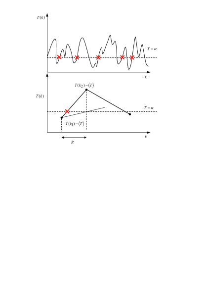
Since we consider the statistical isotropy and homogeneity of temperature random field on the surface, without losing generality, we assume a one-dimensional slice of temperature fluctuations on a patch of CMB with size parallel to or axes. The size of this signal depends on the resolution of data set which is simulated or observed depicted by . Also the numbers of pixels will be . Now consider a sample of an ensemble of one dimensional signal of temperature fluctuation, , for which runs from to . Suppose denotes the numbers of positive slope crossings (upcrossings) of, , for a typical sample size (see Figure (2) ). The ensemble averaging for level crossing with positive slope is also given by:
| (2) |
For a statistical isotropic and homogenous fluctuation, the ensemble averaging can be done on various one dimensional slices of fluctuations. For convenience, we chose these slices to be parallel to or axes. Furthermore, the average number of crossings is proportional to the space (time) interval percy00 . Hence:
| (3) |
which is the average frequency of positive slope crossing of the level . It must be pointed out that in the long run processes the conservation law for upcrossings and downcrossings will be satisfied percy00 . In our analysis due to the statistical isotropy and 200 numbers of run over ensembles or even more, this conservation law statistically holds and so, we use the upcrossing events throughout our analysis.

From mathematical and statistical points of view, the frequency parameter can be
deduced from the probability distributions associated with the temperature fluctuations,
. In order to calculate this probability distribution function, we assume two necessary and sufficient conditions for crossing the level by the underlying signal with positive slope as follows:
1) At the beginning of the interval we should have .
2) The slope of signals should be larger or at least equal to the
slope of line which is drawn between the point at the beginning of
interval and the point located on the horizontal line of level
(Figure (2)), namely:
| (4) |
where . If the above-mentioned conditions are satisfied percy00 ; movahed06 ; movahed05 ; movahed07 ; tabar02 ; tabar03 , we statistically expect to get a high probability for a crossing in the interval . In order to determine whether the above conditions are satisfied at any arbitrary location , we should find how the values of and are distributed by considering their joint probability density function, . For a specific level and interval , we focus on the values of and values of , corresponding to the region between the lines and in the plane () (see Figure (3)). Subsequently, the probability of positive slope crossing of signal at level in the interval is given by:
| (5) |
When , it is legitimate to put:
| (6) |
Since at large values of and , the probability density function approaches zero fast enough, Eq.(5) may be written as:
| (7) |
In this form, the integrand does not depend on so the first integral can be integrated easily:
| (8) |
Figure (3) shows the area of interest for probability of upcrossings at level . As mentioned before, the average number of crossing with positive slope in interval is . So the average number of positive crossings of in interval is equal to the probability of positive crossings of in . We can write the average number of upcrossings at the level in terms of the joint probability density function as follows:
| (9) |
or
| (10) |
Another useful parameter based on can be introduced as:
| (11) |
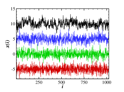
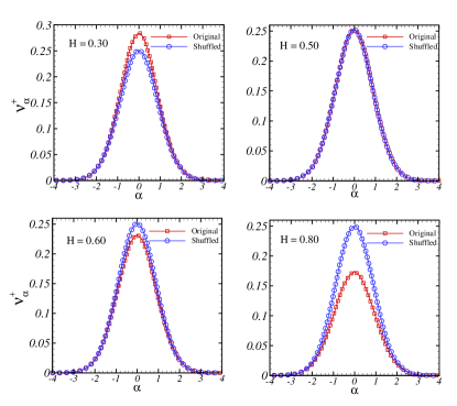
Obviously, for the above quantity determines total number of upcrossings for temperature fluctuations with positive slope at all levels. For a typical rough fluctuation, is larger than that of the smooth signal and consequently, this quantity is a criterion for the roughness of the processes. For a correlated signal, is smaller than that of a completely random one, while for anti-correlated data set is larger than the same series for which its memories have been destroyed by shuffling. Figure (4) shows the level crossing results for some fractional Gaussian noises (fGn) and the corresponding shuffled signals. For an anti-correlated series the so-called Hurst exponent is , for a completely random Gaussian data set and for a correlated signal bunde ; movahedsun . In addition, for moments , those terms in will become dominant that have small deviations from mean level, , which demonstrate the statistics of small fluctuations. On the contrary, for , those terms with large fluctuations in the integrand of Eq.(11) are dominant in explaining the statistical properties of the upcrossings far from mean level. These terms correspond to the rare events.
In what follows, we are going to derive
for discrete temperature fluctuations in the simulated map with and without cosmic strings on the flat sky and compare them to find a robust criterion to distinguish pure Gaussian fluctuations from fluctuations containing cosmic string components. The motivation of using this simple method can be justified according to the following reasons:
i) Since the statistical isotropy is valid as a major statistical property amir1 ; amir2 ; sadeghaniso , one can cut many
one-dimensional signals in every directions and by ensemble averaging, compute the frequency of upcrossings (downcrossings) at all
interested levels along with their variances.
ii) As one can see in the next section, the superposition of fluctuations produced by
cosmic strings can generate new and extra ups and downs in temperature fluctuations, consequently finding such
statistically meaningful footprints in the map in comparison with pure Gaussian signature including instrumental noise may potentially help
us to get deep insight in the cosmic string detections.
iii) Due to the phase coefficient in the Fourier analysis, it seems that many trivial imprints of cosmic strings
diminish or at least are mixed with other observational phenomena so it is another motivation to investigate the imprint of cosmic strings in the real space as mentioned in Ref. brand080 .

III Simulation of Mock CMB map
In this section, we describe in detail our sate-of-the-art code which has been written in Fortran language by authors to simulate temperature fluctuations maps (also for more details see refs brand080 ; brand081 ; brand09 ; pre93 ; pre93a ; pre93b ). Generally, our program has four parts: The first part creates pure Gaussian fluctuations corresponding to the standard inflationary model in the presence of various models governing the evolution of background. In this paper we use CDM model in the flat Universe. Nevertheless, our program can be easily modified to other cosmological models governing the background evolution of universe such as quintessence model and so on sadeghquin . The second part contains anisotropies produced by long cosmic strings by means of Kaiser-Stebbins effect. The superposition of Gaussian and cosmic strings anisotropies as well as the expected instrumental noise are produced in the third part. The normalization factor for each component will be computed in this part. Finally, the algorithm for searching the signatures of cosmic string relying on the level crossing analysis is given in the last part. To find more reliable results and reduced statistical errors, an ensemble averaging over at least 200 runs for a set of input variables will be done. As one can see in the following, we need a fine resolution map. However the random behavior of cosmic strings limits our simulation on the flat sky map approximation brand081 ; white99 ; seljak97 . In this case the Fourier modes are bases functions instead of being spherical harmonics. Before going further, for pedagogical purposes, we summarize all procedures to be done for map making in Figure (5).
III.1 Gaussian map on the Flat sky
In this subsection a Gaussian map for temperature fluctuations will be generated. We use CDM model and the best fit values have been inferred based on the most recent observations such as WMAP-7, Supernova type Ia gold sample (SNIa) and Sloan Digital Sky Survey (SDSS) with the most familiar initial power spectrum established by standard inflationary scenario WMAP7 ; WMAP71 . As discussed in details in Refs. brand080 ; brand081 and indicated in Figure (5), first of all, we should determine the values of initial parameters relevant to the Gaussian map. A part of these parameter are related to the cosmological frame-work and others are the size of simulated map, , angular resolution, , and finally the variance of instrumental noise, namely . Since we are interested in flat sky, namely a simulated map with size less than , two-dimensional plane wave (Fourier basis functions) are used instead of spherical harmonics. The stochastic temperature fluctuations field on the flat sky will be written as:
| (12) |
Actually to guaranty the Gaussianity of distribution based on central limit theorem, we add and as two independent Gaussian random numbers with zero mean and unit variance. The factor in the denominator stands for canceling the corresponding variance of Gaussian random numbers. To set the value of for a given set of in inverse degrees, one can compute as: . The initial power spectrum, , is determined by running CAMB softwarebrand081 ; CAMB . The power spectrum for non-integer values of can be evaluated by linear interpolation in the produced . To this end we modify the public CAMB software for underlaying theoretical model and set the best fit values of corresponding cosmological parameters based on constraints given by the most recent observations. Finally to keep the statistical isotropy and to diminish the undesired preferred direction appearing in simulation, we construct four independent Gaussian maps and superimpose these separate components according to brand080 :
| (13) |
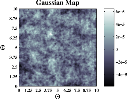
The pre-factor is necessary to keep the initial standard deviation. As mentioned before, in this paper we simulate Gaussian temperature fluctuations based on CDM WMAP7 ; WMAP71 including best fit values for cosmological parameters based on WMAP-7 observations. Figure (6) shows a typical simulated Gaussian map for CDM model.
III.2 Fluctuations Produced by Cosmic Strings
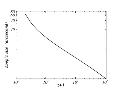
In this subsection we explain in detail the algorithm used for generating cosmic strings by using the Kaiser-Stebbins effect which originally discussed by Perivolaropoulos pre93b ( for more details see Refs. brand081 ; brand080 ; brand09 ; pre93 ; pre93b ; pre93a ). In our toy model, since the size of a typical loop of string is about allen90 ; david88 (see Figure (7)) and the resolution of simulated map is of the order of one arc-minute so we can ignore the contribution of these closed strings and suppose that the main anisotropy in the string map is due to the straight cosmic strings. In addition, it has been shown that loops contribute to temperature fluctuations via the well-known Sachs-Wolfe effect and due to the small bandwidth of simulated map the overall effects can be represented as Gaussian noise sachs67 ; pre93a .
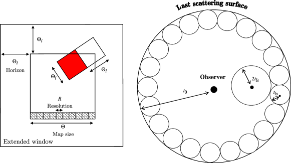
The scaling behavior of the correlation length scale of straight strings demonstrates that the number of strings crossing a given Hubble volume to be fixed. In another word the number density of strings to be invariant under rescaling of correlation length scale allen01 ; allen90 ; ander03 ; arms99 ; david88 ; land03 ; urr07 . Therefore, one can deduce the numbers of straight strings crossing each Hubble volume at any given time to be . Their overall properties such as orientations and velocities are statistically uncorrelated for length scale larger than the corresponding horizon scale david88 ; allen90 ; cope92 . The time interval in our simulation is limited to the interval and since the cosmic strings have relativistic velocity, one can suppose that after ( is Hubble time), a new Hubble volume will be generated and consequently a new network of cosmic strings affects the propagation of the photons transmitted freely after last scattering surface based on the Keiser-Stebbins phenomenon. This is also justified regarding the fact that a photon ray travels most of the Hubble volume during twice the Hubble time, and after that this ray encounters a new volume and will be affected by a new string network. So one can suppose that at successive time intervals according to the relation, , the photon ray could be affected by a new string network. According to this statement, the number of separate string networks (patches) to be simulated is given by (see Figure (8)):
| (14) |
In the string map for the recursion condition, , we let the new network of cosmic strings to kick the photon paths. The apparent angular size of horizon at is given by:
| (15) |
here is , and for flat, closed and open universe, respectively. In the above equation, is the Hubble parameter and includes all model parameters. The number of straight cosmic strings with size at which should be simulated and placed randomly on the desired simulated map will be brand081 ; brand080 ; brand09 ; pre93 :
| (16) |
where is the size of simulated map with resolution equal to , consequently the number of pixels for extended map at th step of simulation is . Actually, to retain all fluctuations produced by cosmic string in a limited area of sky which has been simulated we establish an extended area for each step. The size of mentioned extended window will be at th patch and our simulated map to be considered at the center of this window. Left panel of figure (8) shows this configuration for fluctuations produced by Kaiser-Stebbins phenomena on the cosmic background radiation fluctuations. Upon the calculation of the size of horizon for th successive step by using Eq. (15), we embed a straight string and apply a shift for temperature fluctuations according to Eq.(1). Since the mean value of fluctuations in the simulated map has no physical significance, we add half of to one side of string and subtract the remaining value from other side, namely we use
| (17) |
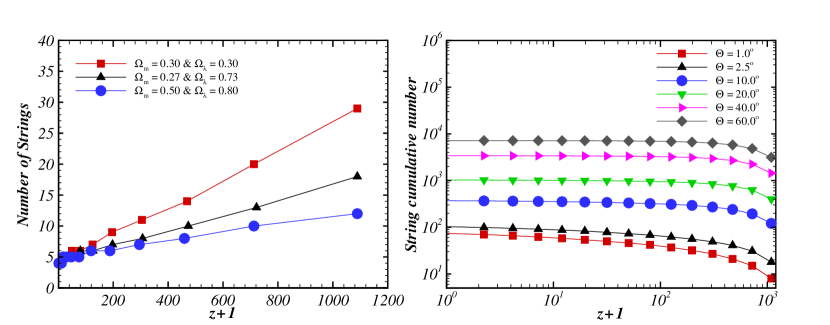
where . The direction of observer for a small field in the map is approximately constant. Since the string’s velocities and orientations are random and furthermore takes into account the contribution of orientation and projection effect of cosmic string, consequently its value will be given by generating a uniform random number over the interval . In addition a binary flag is produced to decide which side of string to be positive and which one will be negative for temperature fluctuations. The location of string in the extended window is also demonstrated by an additional proper random number. We take into account the contribution of projection from 3-dimensions to 2-dimensions of cosmic string by multiplying the proper size of strings at each patch by the cosine of the angle deriving from interval randomly. We fix the relevant coefficient for string simulation e.g. the number of cosmic string for each Hubble volume, and alb85 . It must be pointed out that the fixed values for string quantities change significantly from one theoretical model to the other, consequently in this toy model, we take most popular values for mentioned relevant quantities vilinkin00 . As shown in Figure (9) the number of strings for each step depends on the size of simulated map as well as the underlying cosmological theory. Finally, temperature fluctuations simulated for various patches should be superimposed to reach the final situations for a given pixel in the simulated map. Figure (10) displays a string map for which the cosmic tension is . As an additional check for consistency of our simulation we compute the power spectrum of our pure string simulated map for different values of as well as pure Gaussian generated map in small angle approximation white99 ; mark09 ; spergel08 .
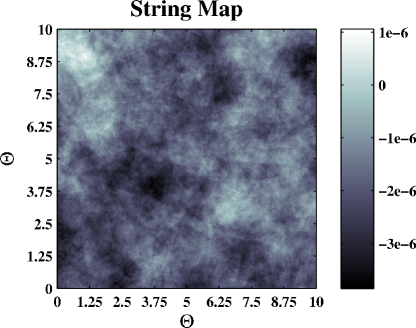
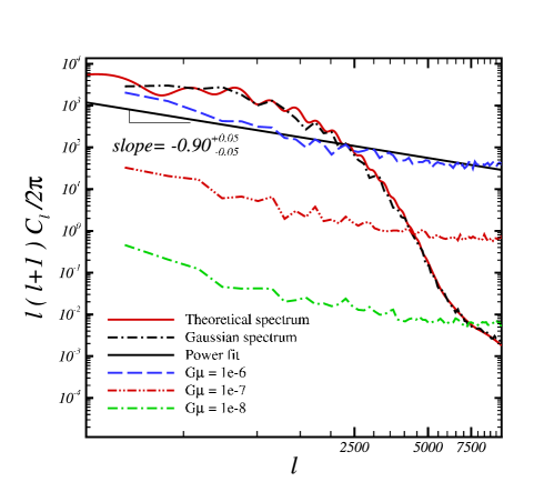
Figure (11) indicates the angular power spectrum for pure Gaussian and pure cosmic string simulated maps for typical field of view of and a resolution of . Since the size and resolution of generated map is finite and temperature fluctuations are limited to the flat sky, the multiple moment will run from to . In addition the expected scaling behavior for pure cosmic string map satisfies the relation for with . Let us explain the final task regarding the simulation of a Gaussian map including induced cosmic string and instrumental noise. As discussed before we simulate all components separately and according to the linear perturbation theory, we superpose all sources to include all phenomena and reach the final situation. We do not expect the observed temperature power spectrum to be changed in the presence of cosmic string, consequently the multiplication by a factor, less than unity causes the power spectrum to remain unchanged. The instrumental noise does not modify the real sky map and its significance is demonstrated by the maximum amplitude of noise represented by . This maximum will be taken as throughout this paper according to the anticipated instrumental noise in South Pole Telescope (SPT) SPT . To finalize our simulation, we use the same method explained in Ref. brand081 . The power spectrum of simulated map can be read as follows:
| (18) |
The cross-correlated term is zero due to independency of Gaussian and string components. We demand the left hand side of the above equation to be equal to power spectrum derived from observation, given by CAMB software. Therefore for each from to , we find a separate ’s. To compute a single , we rely on Bayesian statistics for observations, and model parameters, . We define fab04 : . Here is computed directly from Eq.(18) and derived by an arbitrary merit function which is supposed to be a first order polynomial function throughout this paper.
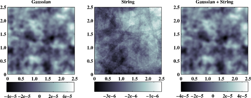
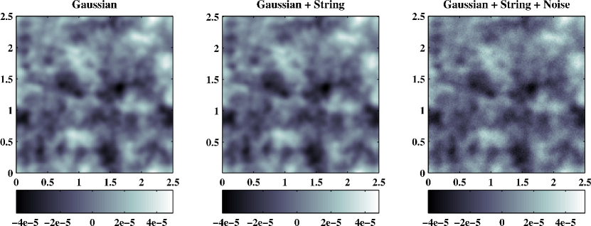
The y-intercept of merit function will be assumed as a best fit value of brand081 . It must be pointed out that to improve the reliability of , we do various simulations and finally by ensemble averaging, an averaged value for can be retrieved. Figure (12) indicates different components simulated without expected instrumental noise. Figure (13) shows simulated map including instrumental noise. Now every things ready to investigate temperature fluctuations on the flat sky with and without cosmic strings. We rely on a robust statistical method namely, level crossing analysis to explore the capability of our method to detect the cosmic strings for various values of string’s tensions.
IV Analysis of CMB Map
As explained in details in section II, we are interested in upcrossings the temperature fluctuations at an arbitrary level, . Or according to probability point of view, we should compute the volume of joint probability density function which is satisfied in the proper conditions mentioned in section II (see Figure (3)). We expect the fluctuations in the presence of cosmic strings to be rougher than pure Gaussian fluctuations. Since the level crossing analysis is applicable for one-dimensional series we construct -dimensional series from simulated map. Furthermore due to the statistical isotropy property of simulated map amir1 ; amir2 ; sadeghaniso , the -dimensional data sets will be created in all given directions as different ensembles for analysis. Actually these series contain temperature fluctuations as a function of pixels in one dimension in an arbitrary direction. Hereafter we turn to investigate -dimensional signals as an input for level crossing subroutine which is the final part of the main simulation program. We introduce the increment of fluctuation as:
| (19) |
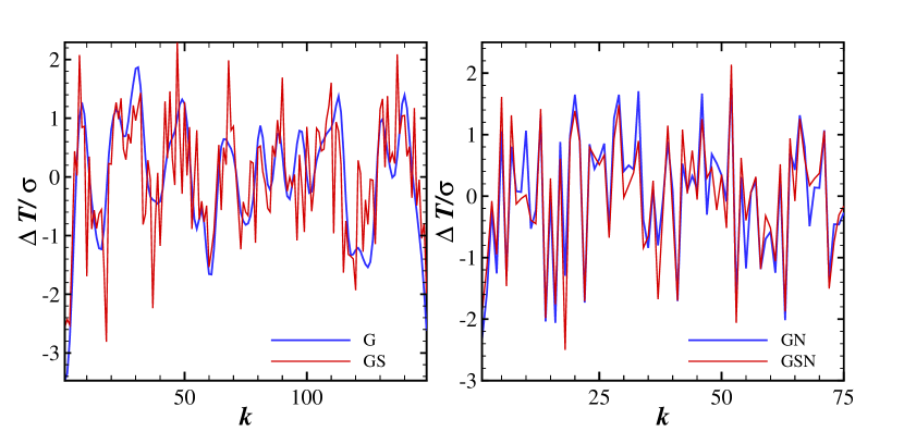
In Figure (14) we have plotted a typical -dimensional increment series for Gaussian and cosmic string signals embedded in Gaussian fluctuations. We see that in the presence of strings, fluctuations near the mean as well as far from the mean have been changed. The magnitude of these changes depends on value of cosmic string tension. As pointed out before, we enumerate the number of crossings with positive slope at whole existence level for all -dimensional data set in a map for a given . It is worth noting that according to conservation law, for long-run simulation all crossings with negative slope are statistically equivalent to that of with positive slope percy00 . Based on this analysis, we find many quantities which may be potentially used as a criterion to distinguish between the maps with and without straight cosmic strings. In Figure (15) we plot the versus for various values of . Generally, total crossings in the Gaussian map is less than that of with cosmic string. As we expect, the existence of instrumental noise decreases the efficiency of our analysis. To compare simulated maps we refer to the generalized form of roughness of signals which is given by Eq.(11), . The various values for ’s take into account crossings with different measures in the total level crossings. Figure (16) indicates the generalized roughness function for some typical values of . To compare the value of generalized roughness function we apply Student’s t-test for equal sample size and unequal mean and standard deviation for each ’s which is defined by:
| (20) |
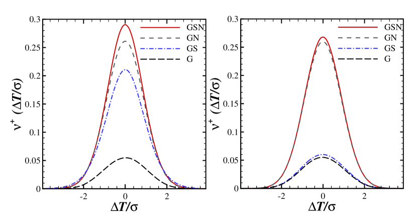
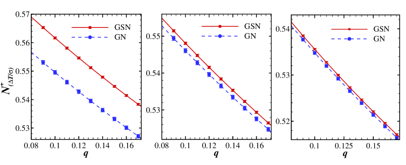
here the symbols and stand for (G) and (GS) for simulated map without noise, respectively. For simulation including instrumental noise these symbols are replaced by (GN) and (GSN), respectively. The is the ensemble average of generalized roughness function for each ’s. The corresponding standard deviation is given by . indicates the number of simulated ensembles. The P-value, for based on t-distribution function with degrees of freedom, will be determined. By the combination of above P-values we introduce the following quantity:
| (21) |
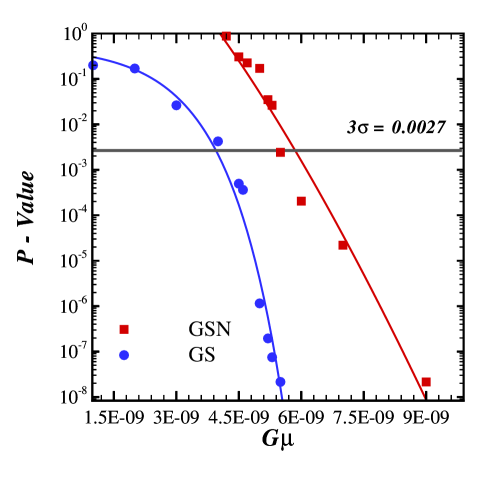
Finally, the last P-value, associating to the by using chi-square distribution function for degrees of freedom will be computed. For significance level namely , we can conservatively say that there exists a significance difference. According to the value of indicated in Figure (17), we conclude that our method can detect the cosmic string with and in the presence of anticipated instrumental noise the lower bound is . The final strategy for detecting cosmic string is as follows: At first by using a map from observation we compute and . Second we simulate a pure Gaussian map with expected instrumental noise and again the level crossing and generalized roughness functions to be calculated. The P-value for deciding about the existence of significant difference between for real and simulated Gaussian maps will be determined. In the case of significant difference, we change the value of for simulated Gaussian map including cosmic strings and compute the corresponding . Upon the for simulation to be equal to that of given for observation we conservatively can express the existence of cosmic strings in the observed map with mentioned .
V Summary and Conclusions
In this paper we relied on a robust method in complex system which has been introduced originally to investigate the statistical properties of -dimensional surface by mapping to -dimensional data sets percy00 ; movahed06 ; movahed05 ; movahed07 ; tabar02 ; tabar03 . Using this method we explore the capability of finding the footprints of straight cosmic string based on the KS effect on the cosmic microwave background fluctuations since the last scattering epoch up to now. To this end we take a simple toy model to simulate the effect of cosmic strings demonstrated in Refs. pre93 ; pre93b . The contribution of loops in this model can be ignored (see Figure (7)). The superposition of kicks due to the embedded cosmic strings cause some additional statistical fluctuations in simulated map. Consequently there exists a difference between the number of level crossing for whole reachable level in -dimensional fluctuations of pure Gaussian map in comparison with map containing cosmic strings. To quantify this deviation we introduced an increment signal and use robust quantity to take into account all deviations relative to pure Gaussian fluctuations, namely generalized roughness function. For the generalized roughness function corresponds to sum of upcrossings at all fluctuation levels which is a measure of roughness of underlying signals. Based on joint probability density function of signal, , we found that the fluctuations near the mean fluctuations could be a proper criterion to discriminate pure Gaussian map from the map induced by cosmic strings. Our result shows that level crossing analysis could place a bound for cosmic string tension for 200 simulated maps with . To explore the contribution of instrumental noise we relied on South Pole Telescope experiment and took for noise map. The new bound for map including instrumental noise is . The small change in the bound on due to the noise could be justified regarding Figure (15). The sensitive part of is crossing near the mean value so the presence the undesired noise can only have minor statistical effects on the ability of this model to place a lower bound on the string’s tension for small value of . In addition, our results for both simulations were not affected by increasing the size of ensemble up to 200 corresponding to increase the coverage of sky map. For the realistic observations there are additional problems to be addressed. The first one is the foreground and the instrumental noise which is supposed to be considered by adding expected noise and smoothing our simulation. As mentioned in Refs. brand081 ; brand080 ; brand09 discontinuity related to the scanning strategy also puts extra imprint on data set. It must point out that our method is sensitive to overall fluctuations in all directions, therefore, since it is expected that by increasing the coverage of underlying map the statistics of fluctuations near the mean to be significant, the mentioned spurious phenomenon will have a negligible contribution to the final result. However we can remove all parallel discontinuities in preferred direction imposed by scanning maneuvering of observational instrument brand081 . Final remark is that we would like to use more realistic models land03 ; spergel08 ; shellard10 to simulate a map taking all contributions of cosmic strings on the cosmic microwave background into account and implement our method to explore the effect of cosmic strings in our future works. In addition as a future study, it is useful to apply this method to distinguish the effect of generic cosmic strings and superstrings on the temperature fluctuations. The n-point peak-peak correlation function is also another method which could be used for the same purpose.
Acknowledgements
We would like to thank H. Firouzjahi and H. Mos’hafi for useful comments and reading manuscript. Also we thank the anonymous referee for his/her useful recommendations and comment regarding the peak-peak correlation function method. M. Sadegh Movahed is grateful to the school of astronomy (IPM) for their hospitality. This work has been partly supported by IPM.
References
- (1) N. Bevis, Mark Hindmarsh, Martin Kunz and Jon Urrestilla, Phys. Rev. Lett. 100, (2008) 021301, astro-ph/0702223.
- (2) N. Bevis, Mark Hindmarsh, Martin Kunz and Jon Urrestilla, Phys. Rev. D. 82, (2010) 065004, arXiv:1005.2663.
- (3) Matthew DePies, Proquest Dissertations And Theses 2009. Section 0250, Part 0606 140 pages; [Ph.D. dissertation].United States – Washington: University of Washington; 2009. Publication Number: AAT 3370485. Source: DAI-B 70/08, Feb 2010, arXiv:0908.3680.
- (4) M. Hindmarsh and T. Kibble, Rept. Prog. Phys. 58:477-562,1995, hep-ph/9411342.
- (5) M. Sakellariadou, Lect. Notes Phys.718:247-288,2007, hep-th/0602276 (2006).
- (6) T. Vachaspati and A. Vilenkin, Phys. Rev. D 30 2036 (1984).
- (7) E. P. S. Shellard, Nucl. Phys. B283, 624 (1987).
- (8) Maxim Yu Khlopov, ”COSMOPARTICLE PHYSICS”, World Scientific publication (1999).
- (9) A. Vilenkin and E. P. S. Shellard, Cosmic Strings and Other Topological Defects (Cambridge, UK: Cambridge University Press. ISBN 0521654769. pp. 578, 2000); T. W. B. Kibble, Topology Of Cosmic Domains And Strings, J. Phys. A 9, 1387 (1976); Y. B. Zeldovich, Cosmological fluctuations produced near a singularity, Mon. Not. Roy. Astron. Soc. 192, 663 (1980); A. Vilenkin, Cosmological Density Fluctuations Produced By Vacuum Strings, Phys. Rev. Lett. 46, 1169 (1981) [Erratum-ibid. 46, 1496 (1981)];
- (10) A. Vilenkin, Phys. Rep., 121 263 (1985).
- (11) B. Allen, ”Relativistic gravitation and gravitational radiation”, J.-A. Marck, J.-P. Lasota. (Proceedings, Les Houches School of Physics: Astrophysical Sources of Gravitational Radiation), Cambridge Contemporary Astrophysics, 1997, pages 373-417, gr-qc/9604033 (1996).
- (12) E. Copeland, Andrew R Liddle, David H Lyth, Ewan D Stewart, David Wands, Phys. Rev. D 49 (1994) 6410-6433.
- (13) Saswat Sarangi, S.-H. Henry Tye, Phys.Lett. B536 (2002) 185-192.
- (14) S.-H. Henry Tye, Lect. Notes Phys. 737:949-974, 2008, arXiv:hep-th/0610221.
- (15) T. W. B. Kibble, arXiv:astro-ph/0410073.
- (16) Edmund J. Copeland, Robert C. Myers, Joseph Polchinski, JHEP 0406:013,2004, arXiv:hep-th/0312067.
- (17) H. Firouzjahi and S. H. Tye, J. Cosm. Astrop. Phys., 03, 009 (2005).
- (18) F. A. Jenet, G. B. Hobbs, W. van Straten, R. N. Manchester, M. Bailes, J. P. W. Verbiest, R. T. Edwards, A. W. Hotan, J. M. Sarkissian and S. M. Ord, Astrophys. J. 653, 1571 (2006), astro-ph/0609013 (2006).
- (19) M. S. Pshirkov and A. V. Tuntsov, Phys. Rev. D, 81, 083519 (2010), arXiv:0911.4955.
- (20) A. V. Tuntsov and M. S. Pshirkov, Phys. Rev. D, 81, 063523 (2010), arXiv:1001.4580.
- (21) T. Damour and A. Vilenkin, Phys. Rev. D 71, 063510 (2005), arXiv:hep-th/0410222.
- (22) Richard Battye and Adam Moss, arXiv:1005.0479.
- (23) V. L. Oknyanskij, Gravit. Cosmol., Vol. 5, suppl. issue, p. 97 - 102 (1999).
- (24) M. V. Sazhin and M. Yu. Khlopov, Astron. Zh. V. 66, PP. 191-193 (1989).
- (25) V. A. Gasilov, V. I. Maslyankin and M. Yu. Khlopov, Astrofizika (1985), V.23, PP.191-201. [English translation: Astrophysics, V.23, NO.1/JAN, PP. 485-491, 1986].
- (26) S. I. Blinnikov and M. Yu. Khlopov, Yadernaya Fizika (1982) V. 36, PP. 809-811. [English translation: Sov.J.Nucl.Phys. (1982) V. 36, PP. 472-474].
- (27) J. L. Christiansen, E. Albin, J. Goldman, I.P.W. Teng, M. Foley, G.F. Smoot, arXiv:1008.0426.
- (28) R. H. Brandenberger, Rebecca J. Danos, Oscar F Hernandez, Gilbert P. Holder, arXiv:1006.2514.
- (29) D. M. Regan and E. P. S. Shellard, Phys. Rev. D. 82 (2010) 063527, arXiv:0911.2491.
- (30) Mark Hindmarsh, Christophe Ringeval and Teruaki Suyama, Phys. Rev. D 80, 083501 (2009).
- (31) Aurelien A. Fraisse, Christophe Ringeval, David N. Spergel and Francois R. Bouchet, Phys. Rev. D 78, 043535 (2008).
- (32) N. Kaiser and A. Stebbins, Nature 310, 391 (1984).
- (33) A. A. Fraisse, arXiv:astro-ph/0503402.
- (34) N. Bevis, M. Hindmarsh and M. Kunz, Phys. Rev. D 70, (2004) 043508.
- (35) N. Bevis, M. Hindmarsh, M. Kunz and J. Urrestilla, Phys. Rev. D 75, 065015 (2007).
- (36) M. Wyman, L. Pogosian and I. Wasserman, Phys. Rev. D 72, 023513 (2005).
- (37) M. Wyman, L. Pogosian and I. Wasserman, Phys. Rev. D 73, 089905(E) (2006).
- (38) L. Perivolaropoulos, Phys. Lett. B 298, 305 - 311 (1993).
- (39) Ligo and Virgo collaboration, Nature, 460, 20 (2009).
- (40) Daisuke Yamauchi, Yuuiti Sendouda, Chul-Moon Yoo, Keitaro Takahashi, Atsushi Naruko and Misao Sasaki, arXiv:1004.0600.
- (41) Yin-Zhe Ma, Wen Zhao and Michael L. Brown, JCAP 10 (2010) 007.
- (42) D. K. Hammond, Y. Wiaux and P. Vandergheynst, Mon. Not. R. Astron. Soc. 398 (2009) 1317, arXiv:0811.1267.
- (43) R. B. Barreiro and M. P. Hobson, MNRAS, 327, 813 (2001).
- (44) R. B. Barreiro, E. Martinez-Gonzalez, P. Vielva and M. P. Hobson, MNRAS, 368, 226 (2006).
- (45) E. Jeong, Carlo Baccigalupi and G. F. Smoot, JCAP, 09, pp. 018 (2010), arXiv:1004.1046.
- (46) R. J. Danos and R. H. Brandenberger, Int.J.Mod.Phys.D19:183-217,2010, arXiv:0811.2004.
- (47) A. Stewart and R. H. Brandenberger, JCAP, 02, pp. 009 (2009), arXiv:0809.0865.
- (48) R. J. Danos and R. H. Brandenberger, JCAP, 02, pp. 033 (2010), arXiv:0910.5722.
- (49) J. L. Starck, N. Aghanim and O. Forni, Astron.Astrophys. 416 (2004) 9-17, arXiv:astro-ph/0311577.
- (50) Christophe Ringeval, Advances in Astronomy, vol. 2010, Article ID 380507, 28 pages, 2010.
- (51) J. A. Peacock and Alan F. Heavens, Mon.Not.Roy.Astron.Soc. 217 (1985) 805.
- (52) J. M. Bardeen, J. R. Bond, N. Kaiser and A. S. Szalay, ApJ, 304 (1986) 15.
- (53) Alan F. Heavens and Ravi K. Sheth, Mon.Not.Roy.Astron.Soc. 310 (1999) 1062.
- (54) Alan F. Heavens and Sujata Gupta, Mon.Not.Roy.Astron.Soc. 324 (2001) 960.
- (55) N. Aghanim, S. Prunet, O. Forni and F. R. Bouchet, arXiv:astro-ph/9803040.
- (56) A. Stebbins, The Astrophysical Journal, 327, 584-614 (1988).
- (57) M. Birkinshaw and S. F. Gull, Nature, 302, 24 (1983).
- (58) M. Birkinshaw, ”Moving gravitational lenses”, Lectutre notes in physics, Vd. 330, 1989, P. 56, Springer- Verlag.
- (59) S. O. Rice, Bell System Tech. J. 23 282 (1944); ibid. 24 46 (1945).
- (60) Percy H. Brill, CORS Bulletin Vol. 34, 4 (2000).
- (61) M. Sadegh Movahed, A. Bahraminasab, H. Rezazadeh and A. A. Masoudi, J. Phys. A: Math. Gen. 39, 3903 (2006).
- (62) A. Bahraminasab, M. Sadegh Movahed, S. D. Nasiri and A. A. Masoudi, Journal of Statistical Physics, Vol. 124, No. 6, (2006).
- (63) G. R. Jafari, M. Sadegh Movahed, S. M. Fazeli, M. Rahimi Tabar and A. F. Masoudi, J. Stat. Mech (2006), P06008.
- (64) A. A. Masoudi, F. Shabazi, J. Davoudi, M. R. Rahimi Tabar, Phys. Rev. E 65, 026132 (2002).
- (65) F. Shahbazi, S. Sobhanian, M. R. Rahimi Tabar, S. Khorram, G. R. Frootan, H. Zadeh, J. Phys. A 36, 2517 (2003).
- (66) J. W. Kantelhardt, S.A. Zschiegner, E. Koscielny-Bunde, A. Bunde, S. Havlin, H.E. Stanley, Physica A 316 (2002) 87.
- (67) M. Sadegh Movahed, G. R. Jafari, F. Ghasemi, S. Rahvar, M. Rahimi Tabar, J. Stat. Mech. (2006) P02003.
- (68) A. Hajian and T. Souradeep, Astrophys. J. 597, L5 (2003).
- (69) A. Hajian and T. Souradeep, Phys. Rev. D 74, 123521 (2006).
- (70) M. Sadegh Movahed, F. Ghasemi, Sohrab Rahvar, M. Reza Rahimi Tabar, arXiv:astro-ph/0602461.
- (71) R. Moessner, L. Perivolaropoulos and R. Brandenberger, Ast. Phys. J. 425, 365 - 371 (1994).
- (72) L. Perivolaropoulos, Phys. Rev. D 48, 4 (1993).
- (73) S. Rahvar and M. Sadegh Movahed, Phys. Rev. D 75, 023512 (2007).
- (74) Matias Zaldarriaga and Uros Seljak, Phys. Rev. D, 55, 1830-1840 (1997).
- (75) M. White, J. Carlstrom, M. Dragovan, and W. Holzapfel, Astrophys. J. 514, 12 (1999).
- (76) E. Komatsu et al., arXiv:1001.4538.
- (77) D. Larson et al., arXiv:1001.4635.
- (78) A. Lewis, A. Challinor and A. Lasenby, ”Efficient Computation of CMB anisotropies in closed FRW models”, Astrophys. J. 538, 473 (2000), arXiv:astro-ph/9911177.
- (79) David P. Bennet and Frencois R. Bouchet, Phys. Rev. Lett. 60, 4 (1988).
- (80) B. Allen and E. P. S. Shellard, Phys. Rev. Lett. 64, 119 (1990)
- (81) R. Sachs and A. Wolfe, ApJ, 147, 3 (1967).
- (82) M. Anderson, ”The Mathematical Theory of Cosmic Strings”, (Institute of Physics Publishing, London, 2003).
- (83) J. W. Armstrong, F. B. Estabrook and M. Tinto, Astrophys. J., 527, 814 (1999).
- (84) M. Landrian and E. P. S. Shellard, Phys. Rev. D 67, 103512 (2003).
- (85) J. Urrestilla and Alexander Vilenkin, JHEP0802:037,2008, arXiv:0712.1146.
- (86) B. Allen and A.C. Ottewill, Phys. Rev. D 63, 063507 (2001).
- (87) E. Copeland, T. W. B. Kibble and Daren Austin, Phys. Rev. D 45, 4 (1992).
- (88) A. Albrecht and N. Turok, Phys. Rev. L 54, 1868 (1985).
- (89) J. E. Ruhl et al. (The SPT) (2004), arXiv:astro-ph/0411122.
- (90) R. Colistete Jr., J.C. Fabris, S.V.B. Goncalves, P.E. de Souza, Internat J. Modern Phys. D 13 (2004) 669.
- (91) M . Landriau and E. P. S. Shellard, arXiv:1004.2885.