Horizon dynamics of distorted rotating black holes

Abstract

We present numerical simulations of a rotating black hole distorted by a pulse of ingoing gravitational radiation. For strong pulses, we find up to five concentric marginally outer trapped surfaces. These trapped surfaces appear and disappear in pairs, so that the total number of such surfaces at any given time is odd. The world tubes traced out by the marginally outer trapped surfaces are found to be spacelike during the highly dynamical regime, approaching a null hypersurface at early and late times. We analyze the structure of these marginally trapped tubes in the context of the dynamical horizon formalism, computing the expansion of outgoing and incoming null geodesics, as well as evaluating the dynamical horizon flux law and the angular momentum flux law. Finally, we compute the event horizon. The event horizon is well-behaved and approaches the apparent horizon before and after the highly dynamical regime. No new generators enter the event horizon during the simulation.

I Introduction

In the efforts by the numerical relativity community leading up to the successful simulation of the inspiral and merger of two black holes, analyses of single black holes distorted by gravitational radiation have offered a convenient and simpler setting to understand the nonlinear dynamics during the late stages of binary black hole coalescence. For this purpose, initial data for a Schwarzschild black hole plus a Brill wave was presented in Bernstein et al. (1994), which was both time symmetric and axisymmetric. In highly distorted cases, the apparent horizon could develop very long, spindlelike geometries. If the event horizon can show similar behavior, this would raise intriguing questions related to the hoop conjecture Thorne (1972). The work of Bernstein et al. (1994) was extended to distorted rotating black holes in Anninos et al. (1994), where the apparent horizon served as a useful tool to examine the quasinormal oscillations of the black hole geometry as it relaxed in an evolution. Further studies have extracted the gravitational waves emitted by the black hole Brandt and Seidel (1995), and compared the apparent and event horizons Anninos et al. (1995).

We continue this line of investigation here, while incorporating various modern notions of quasilocal horizons that have emerged in recent years. Our emphasis is on horizon properties during the highly dynamical regime, and no symmetries are present in our initial data and evolutions. The utility of quasilocal horizons can be immediately appreciated when one wants to perform a numerical evolution of a black hole spacetime. One must be able to determine the surface of the black hole at each time, in order to track the black hole’s motion and compute its properties, such as its mass and angular momentum. However, the event horizon, which is the traditional notion of a black hole surface, can only be found after the entire future history of the spacetime is known.

Quasilocal horizons can be computed locally in time, and so are used instead to locate a black hole during the evolution. Of particular interest is a marginally outer trapped surface (MOTS), which is a spatial surface on which the expansion of its outgoing null normal vanishes Hawking and Ellis (1973). The use of MOTSs is motivated by several results. When certain positive energy conditions are satisfied, an MOTS is either inside of or coincides with an event horizon Hawking and Ellis (1973); Wald (1984). The presence of an MOTS also implies the existence of a spacetime singularity Penrose (1965). In an evolution, the MOTSs located at successive times foliate a world tube, called a marginally trapped tube (MTT). MTTs have been studied in the context of trapping horizons Hayward (1994, 2004), isolated horizons Ashtekar et al. (2000a, b, 2001), and dynamical horizons Ashtekar and Krishnan (2002, 2003); Ashtekar and Galloway (2005).

Both the event horizon and an MTT react to infalling matter and radiation, although their behaviors can be quite different in highly dynamical situations. Being a null surface, the evolution of the event horizon is governed by the null Raychaudhuri equation Poisson (2004), so that even though its area never decreases, in the presence of infalling matter and radiation the rate of growth of its area decreases and can even become very close to zero Booth (2005). Since an MTT is determined by quasilocal properties of the spacetime, its reaction to infalling matter and radiation is often much more intuitive. A MTT is usually spacelike (e.g. a dynamical horizon) in such situations, although further scrutiny has revealed that MTTs can exhibit various intriguing properties of their own. For example, an MTT may become timelike and decrease in area Booth et al. (2006), or even have sections that are partially spacelike and partially timelike Schnetter et al. (2006). In a numerical simulation, such behavior is often indicated by the appearance of a pair of new MTTs at a given time, accompanied by a discontinuous jump in the world tube of the apparent horizon, or outermost MOTS.

In this paper, we investigate the behavior of MTTs and the event horizon in the context of a rotating black hole distorted by an ingoing pulse of gravitational waves. First, we construct a series of initial data sets in which the amplitude of the gravitational waves varies from small to large, which are then evolved. We focus on the evolution with the largest distortion of the black hole, in which the mass of the final black hole is more than double its initial value. During the evolution, the world tube of the apparent horizon jumps discontinuously when the gravitational waves hit the black hole, and as many as five MTTs are found at the same time. Some of these MTTs decrease in area with time, although we find that all the MTTs during the dynamical stages of our evolution are spacelike and dynamical horizons. Moreover, all these MTTs join together as a single dynamical horizon. Their properties are further analyzed using the dynamical horizon flux law Ashtekar and Krishnan (2003), which allows one to interpret the growth of the black hole in terms of separate contributions. We also evaluate the angular momentum flux law based on the generalized Damour-Navier-Stokes equation Gourgoulhon (2005). Finally, we locate the event horizon and contrast its behavior with that of the MTTs.

The organization of this paper is as follows. Section II details the construction of the initial data sets and Sec. III describes the evolutions. Section IV introduces some definitions about MOTSs, and the methods used to locate them. Section V discusses the MTTs foliated by the MOTSs, the determination of their signatures, and the fluxes of energy and angular momentum across them. The emphasis is on the case with the largest distortion of the initial black hole, as is the remainder of the paper. Section VI explains how we find the event horizon, and contrasts its properties with the MTTs. Section VII presents some concluding remarks. Finally, the appendix offers some insight on our results in light of the Vaidya spacetime.

II Initial Data

Initial data sets are constructed following the method of Pfeiffer et al. (2005), which is based on the extended conformal thin sandwich formalism. First, the 3+1 decomposition of the spacetime metric is given by Arnowitt et al. (1962); York, Jr. (1979)

$$^{(4)}ds^{2} =g_{\mu\nu}dx^{\mu}dx^{\nu},$$ (1)

$$=-N^{2}dt^{2}+g_{ij}\left(dx^{i}+\beta^{i}dt\right)\left(dx^{j}+\beta^{j}dt\right),$$ (2)

where $g_{ij}$ is the spatial metric of a $t=\text{constant}$ hypersurface $\Sigma_{t}$, $N$ is the lapse function, and $\beta^{i}$ is the shift vector. (Here and throughout this paper, Greek indices are spacetime indices running from 0 to 3, while Latin indices are spatial indices running from 1 to 3.) Einstein’s equations (here with vanishing stress-energy tensor $T_{\mu\nu}=0$) then become a set of evolution equations,

$$(\partial_{t}-\mathcal{L}_{\beta})g_{ij} =-2NK_{ij},$$ (3)

$$(\partial_{t}-\mathcal{L}_{\beta})K_{ij} =N\left(R_{ij}-2K_{ik}{K^{k}}_{j}+KK_{ij}\right)-\nabla_{i}\nabla_{j}N,$$ (4)

and a set of constraint equations,

$$R+K^{2}-K_{ij}K^{ij} =0,$$ (5)

$$\nabla_{j}\left(K^{ij}-g^{ij}K\right) =0.$$ (6)

In the above, $\mathcal{L}$ is the Lie derivative, $\nabla_{i}$ is the covariant derivative compatible with $g_{ij}$, $R=g^{ij}R_{ij}$ is the trace of the Ricci tensor $R_{ij}$ of $g_{ij}$, and $K=g^{ij}K_{ij}$ is the trace of the extrinsic curvature $K_{ij}$ of $\Sigma_{t}$.

Next, a conformal decomposition of various quantities is introduced. The conformal metric ${\tilde{g}}_{ij}$ and conformal factor $\psi$ are given by

$$g_{ij}=\psi^{4}{\tilde{g}}_{ij},$$ (7)

the time derivative of the conformal metric is denoted by

$$\tilde{u}_{ij}=\partial_{t}{\tilde{g}}_{ij},$$ (8)

and satisfies $\tilde{u}_{ij}\tilde{g}^{ij}=0$, while the conformal lapse is given by $\tilde{N}=\psi^{-6}N$. Equations (5), (6), and the trace of (4) can then be written as

$$\tilde{\nabla^{2}}\psi-\frac{1}{8}\psi\tilde{R}-\frac{1}{12}\psi^{5}K^{2}+\frac{1}{8}\psi^{-7}\tilde{A}_{ij}\tilde{A}^{ij}=0,$$ (9)

$$\tilde{\nabla}_{j}\left(\frac{1}{2\tilde{N}}\left(\mathbb{L}\beta\right)^{ij}\right)-\tilde{\nabla}_{j}\left(\frac{1}{2\tilde{N}}\tilde{u}^{ij}\right)-\frac{2}{3}\psi^{6}\tilde{\nabla}^{i}K=0,$$ (10)

$$\tilde{\nabla}^{2}\left(\tilde{N}\psi^{7}\right)-\left(\tilde{N}\psi^{7}\right)\left(\frac{1}{8}\tilde{R}+\frac{5}{12}\psi^{4}K^{2}+\frac{7}{8}\psi^{-8}\tilde{A}_{ij}\tilde{A}^{ij}\right)$$

$$=-\psi^{5}\left(\partial_{t}K-\beta^{k}\partial_{k}K\right).$$ (11)

In the above, $\tilde{\nabla}_{i}$ is the covariant derivative compatible with $\tilde{g}_{ij}$, $\tilde{R}=\tilde{g}^{ij}\tilde{R}_{ij}$ is the trace of the Ricci tensor $\tilde{R}_{ij}$ of $\tilde{g}_{ij}$, $\tilde{\mathbb{L}}$ is the longitudinal operator,

$$\left(\tilde{\mathbb{L}}\beta\right)^{ij}=\tilde{\nabla}^{i}\beta^{j}+\tilde{\nabla}^{j}\beta^{i}-\frac{2}{3}\tilde{g}^{ij}\tilde{\nabla}_{k}\beta^{k},$$ (12)

and $\tilde{A}^{ij}$ is

$$\tilde{A}^{ij}=\frac{1}{2\tilde{N}}\left(\left(\tilde{\mathbb{L}}\beta\right)^{ij}-\tilde{u}^{ij}\right),$$ (13)

which is related to $K_{ij}$ by

$$K_{ij}=\psi^{-10}\tilde{A}_{ij}+\frac{1}{3}g_{ij}K.$$ (14)

For given $\tilde{g}_{ij}$, $\tilde{u}_{ij}$, $K$, and $\partial_{t}K$, Eqs.  (9), (10), and (II) are a coupled set of elliptic equations that can be solved for $\psi$, $\tilde{N}$, and $\beta^{i}$. From these solutions, the physical initial data $g_{ij}$ and $K_{ij}$ are obtained from (7) and (14), respectively.

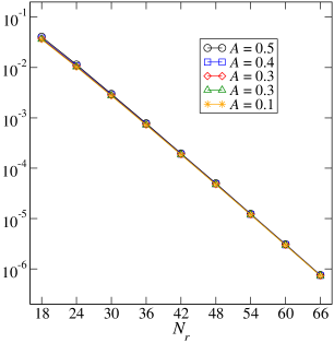
Figure 1: Convergence of the elliptic solver for different amplitudes $A$. Plotted is the square-sum of the Hamiltonian and momentum constraints, Eqs. (5) and (6), as a function of numerical resolution, measured here by the number of radial basis functions in the spherical shell containing the gravitational waves.

To construct initial data describing a Kerr black hole initially in equilibrium, together with an ingoing pulse of gravitational waves, we make the following choices for the free data,

$$\tilde{g}_{ij} =g^{\text{KS}}_{ij}+Ah_{ij},$$ (15)

$$\tilde{u}_{ij} =A\partial_{t}h_{ij}-\frac{1}{3}\tilde{g}_{ij}\tilde{g}^{kl}A\partial_{t}h_{kl},$$ (16)

$$K =K^{KS},$$ (17)

$$\partial_{t}K =0.$$ (18)

In the above, $g^{\text{{KS}}}_{ij}$ and $K^{\text{KS}}$ are the spatial metric and the trace of the extrinsic curvature in Kerr-Schild coordinates, with mass parameter $M_{\text{KS}}=1$ and spin parameter $a_{\text{KS}}=0.7M_{\text{KS}}$ along the $z$-direction. The pulse of gravitational waves is denoted by $h_{ij}$, and is chosen to be an ingoing, even parity, $m=2$, linearized quadrupole wave in a flat background as given by Teukolsky Teukolsky (1982) (see Rinne (2009) for the solution for all multipoles). The explicit expression for the spacetime metric of the waves in spherical coordinates is

$$h_{ij}dx^{i}dx^{j} =\left(R_{1}\sin^{2}\theta\cos 2\phi\right)dr^{2}$$

$$+2R_{2}\sin\theta\cos\theta\cos 2\phi rdrd\theta$$

$$-2R_{2}\sin\theta\sin 2\phi r\sin\theta drd\phi$$

$$+\left[R_{3}\left(1+\cos^{2}\theta\right)\cos 2\phi-R_{1}\cos 2\phi\right]r^{2}d^{2}\theta$$

$$+\left[2\left(R_{1}-2R_{3}\right)\cos\theta\sin 2\phi\right]r^{2}\sin\theta d\theta d\phi$$

$$+\left[R_{3}\left(1+\cos^{2}\theta\right)\cos 2\phi+R_{1}\cos^{2}\theta\cos 2\phi\right]$$

$$\hskip 113.81102pt\times r^{2}\sin^{2}\theta d^{2}\phi,$$ (19)

where the radial functions are

$$R_{1} =3\left[\frac{F^{(2)}}{r^{3}}+\frac{3F^{(1)}}{r^{4}}+\frac{3F}{r^{5}}\right],$$ (20)

$$R_{2} =-\left[\frac{F^{(3)}}{r^{2}}+\frac{3F^{(2)}}{r^{3}}+\frac{6F^{(1)}}{r^{4}}+\frac{6F}{r^{5}}\right],$$ (21)

$$R_{3} =\frac{1}{4}\left[\frac{F^{(4)}}{r}+\frac{2F^{(3)}}{r^{2}}+\frac{9F^{(2)}}{r^{3}}+\frac{21F^{(1)}}{r^{4}}+\frac{21F}{r^{5}}\right],$$ (22)

and the shape of the waves is determined by

$$F =F(t+r)=F(x)=e^{-(x-x_{0})^{2}/w^{2}},$$ (23)

$$F^{(n)} \equiv\left[\frac{d^{n}F(x)}{dx^{n}}\right]_{x=t+r}.$$ (24)

We choose $F$ to be a Gaussian of width $w/M_{\text{KS}}=1.25$, at initial radius $x_{0}/M_{\text{KS}}=15$. The constant $A$ in Eq. (15) is the amplitude of the waves. We use the values $A=0.1$, 0.2, 0.3, 0.4, and 0.5, each resulting in a separate initial data set.

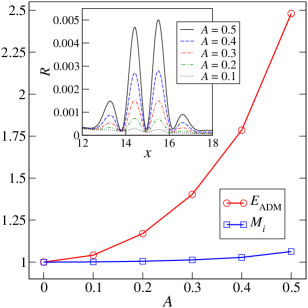
Figure 2: ADM energy $E_{\text{ADM}}$ and Christodoulou mass $M_{i}$ of the initial data sets, versus the gravitational wave amplitude $A$. The inset shows the Ricci scalar $R$ along the $x$-axis. All quantities are given in units of the mass of the background Kerr-Schild metric.

Equations (9), (10), and (II) are solved with the pseudospectral elliptic solver described in Pfeiffer et al. (2003). The domain decomposition used in the elliptic solver consists of three spherical shells with boundaries at radii $r/M_{\text{KS}}=1.5$, 12, 18, and $10^{9}$, so that the middle shell is centered on the initial location of the gravitational wave pulse. The inner boundary lies inside the apparent horizon and Dirichlet boundary conditions appropriate for the Kerr black hole are imposed. It should be noted that these boundary conditions are only strictly appropriate in the limit of small $A$ and large $x_{0}$, when the initial data corresponds to an ingoing pulse of linearized gravitational waves on an asymptotically flat background, with a Kerr black hole at the origin. As $A$ is increased and $x_{0}$ is reduced, we expect this property to remain qualitatively true, although these boundary conditions become physically less well motivated. Nonetheless, we show below by explicit evolution that most of the energy in the pulse moves inward and increases the black hole mass.

At the lowest resolution, the number of radial basis functions in each shell is (from inner to outer) $N_{r}=9$, 18, and 9, and the number of angular basis functions in each shell is $L=5$. At the highest resolution, the number of radial basis functions in each shell is (from inner to outer) $N_{r}=41$, 66, and 41, and the number of angular basis functions in each shell is $L=21$. Figure 1 shows the convergence of the elliptic solver. The expected exponential convergence is clearly visible. Curves for each $A$ lie very nearly on top of each other, indicating that convergence is independent of the amplitude of the waves. We evolve the initial data sets computed at the highest resolution of the elliptic solver.

We locate the apparent horizon (the outermost marginally outer trapped surface defined in Sec. IV.1) in each initial data set using the pseudospectral flow method of Gundlach Gundlach (1998) (explained briefly in Sec. IV.2), and compute the black hole’s initial quasilocal angular momentum $J_{i}$ and Christodoulou mass $M_{i}$ (the subscript “$i$” denotes initial values). The quasilocal angular momentum $J$ is defined in Eq. (48), which we calculate with approximate Killing vectors Lovelace et al. (2008) (see also Cook and Whiting (2007)). The Christodoulou mass $M$ is given by

$$M=\sqrt{{M_{\text{H}}}^{2}+\frac{J^{2}}{4{M_{\text{H}}}^{2}}},$$ (25)

where $M_{\text{H}}=\sqrt{A_{\text{H}}/16\pi}$ is the Hawking or irreducible mass Hawking (1968), with $A_{\text{H}}$ being the area of the marginally outer trapped surface of interest. The main panel of Fig. 2 shows $M$ and the Arnowitt-Deser-Misner (ADM) energy $E_{\text{ADM}}$, as a function of the amplitude $A$ of each initial data set. The difference between $E_{\text{ADM}}$ and $M$ is a measure of the energy contained in the ingoing gravitational waves. For $A\gtrsim 0.4$, this energy is comparable to or greater than $M$, so the black hole will become strongly distorted in the subsequent evolution. The inset of Fig. 2 shows the Ricci scalar $R$ of $g_{ij}$ along the $x$-axis at the initial location of the gravitational wave pulse. The sharp features of $R$ necessitate the use of the higher $N_{r}$ as labeled in Fig. 1.

III Evolutions

Each of the initial data sets are evolved with the Spectral Einstein Code (SpEC) described in Scheel et al. (2006); SpE . This code solves a first-order representation Lindblom et al. (2006) of the generalized harmonic system Friedrich (1985); Garfinkle (2002); Pretorius (2005). The gauge freedom in the generalized harmonic system is fixed via a freely specifiable gauge source function $H_{\mu}$ that satisfies

$$H_{\mu}(t,x)=g_{\mu\nu}\nabla_{\lambda}\nabla^{\lambda}x^{\nu}=-\Gamma_{\mu},$$ (26)

where $\Gamma_{\mu}=g^{\nu\lambda}\Gamma_{\mu\nu\lambda}$ is the trace of the Christoffel symbol. In 3+1 form, the above expression gives evolution equations for $N$ and $\beta^{i}$ Lindblom et al. (2006),

$$\partial_{t}N-\beta^{i}\partial_{i}N =-N\left(H_{t}-\beta^{i}H_{i}+NK\right),$$ (27)

$$\partial_{t}\beta^{i}-\beta^{k}\partial_{k}\beta^{i} =Ng^{ij}\left[N\left(H_{j}+g^{kl}\Gamma_{jkl}\right)-\partial_{j}N\right],$$ (28)

so there is no loss of generality in specifying $H_{\mu}$ instead of $N$ and $\beta^{i}$, as is more commonly done. For our evolutions, $H_{\mu}$ is held fixed at its initial value.

The decomposition of the computational domain consists of eight concentric spherical shells surrounding the black hole. The inner boundary of the domain is at $r/M_{\text{KS}}=1.55$, inside the apparent horizon of the initial black hole, while the outer boundary is at $r/M_{\text{KS}}=50$. The outer boundary conditions Lindblom et al. (2006); Rinne (2006); Rinne et al. (2007) are designed to prevent the influx of unphysical constraint violations Stewart (1998); Friedrich and Nagy (1999); Bardeen and Buchman (2002); Szilágyi et al. (2002); Calabrese et al. (2003); Szilágyi and Winicour (2003); Kidder et al. (2005) and undesired incoming gravitational radiation Buchman and Sarbach (2006, 2007), while allowing the outgoing gravitational radiation to pass freely through the boundary. Interdomain boundary conditions are enforced with a penalty method  Gottlieb and Hesthaven (2001); Hesthaven (2000). The evolutions were run on up to three different resolutions – low, medium, and high. For the low resolution, the number of radial basis functions in each shell is $N_{r}=23$, and the number of angular basis functions in each shell is $L=15$. For the high resolution, $N_{r}=33$ and $L=21$ in each shell.

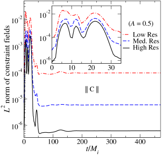
Figure 3: Constraint violations for the evolution with $A=0.5$. Plotted is the $L^{2}$ norm of all constraints, normalized by the $L^{2}$ norm of the spatial gradients of all dynamical fields.

We will be mainly interested in the case where the gravitational waves have an amplitude $A=0.5$. As a measure of the accuracy of this evolution, the constraints of the first-order generalized harmonic system are plotted in Fig. 3. Plotted is the $L^{2}$ norm of all constraint fields, normalized by the $L^{2}$ norm of the spatial gradients of the dynamical fields (see Eq. (71) of Lindblom et al. (2006)). The $L^{2}$ norms are taken over the entire computational volume. The constraints increase at first, as the black hole is distorted by the gravitational waves. As the black hole settles down to equilibrium, the constraints decay and level off. The results presented in the following sections use data from the high resolution runs only.

IV Marginally Trapped Surfaces

IV.1 Basic Definitions and Concepts

Let $\mathcal{S}$ be a closed, orientable spacelike 2-surface in $\Sigma_{t}$. There are two linearly independent and future-directed outgoing and ingoing null vectors $l^{\mu}$ and $k^{\mu}$ normal to $\mathcal{S}$. We write these vectors in terms of the future-directed timelike unit normal $n^{\mu}$ to $\Sigma_{t}$ and the outward-directed spacelike unit normal $s^{\mu}$ to $\mathcal{S}$ as

$$l^{\mu}=\frac{1}{\sqrt{2}}\left(n^{\mu}+s^{\mu}\right)\hskip 5.69054pt\text{and}\hskip 5.69054ptk^{\mu}=\frac{1}{\sqrt{2}}\left(n^{\mu}-s^{\mu}\right),$$ (29)

normalized so that $g_{\mu\nu}l^{\mu}k^{\nu}=-1$. Then the induced metric $\bar{q}_{\mu\nu}$ on $\mathcal{S}$ is

$$\bar{q}_{\mu\nu} =g_{\mu\nu}+l_{\mu}k_{\nu}+l_{\nu}k_{\mu},$$ (30)

$$=g_{\mu\nu}+n_{\mu}n_{\nu}-s_{\mu}s_{\nu}.$$ (31)

The extrinsic curvatures of $\mathcal{S}$ as embedded in the full four-dimensional spacetime are

$$\bar{K}^{(l)}_{\mu\nu}=\bar{q}^{\lambda}_{\mu}\bar{q}^{\rho}_{\nu}\nabla_{\lambda}l_{\rho}\hskip 5.69054pt\text{and}\hskip 5.69054pt\bar{K}^{(k)}_{\mu\nu}=\bar{q}^{\lambda}_{\mu}\bar{q}^{\rho}_{\nu}\nabla_{\lambda}k_{\rho}.$$ (32)

The null vectors $l^{\mu}$ and $k^{\mu}$ are tangent to a congruence of outgoing and ingoing null geodesics, respectively. The traces of the extrinsic curvatures give the congruences’ expansions

$$\theta_{(l)}=\bar{q}^{\mu\nu}\nabla_{\mu}l_{\nu}\hskip 5.69054pt\text{and}\hskip 5.69054pt\theta_{(k)}=\bar{q}^{\mu\nu}\nabla_{\mu}k_{\nu},$$ (33)

and the shears are the trace-free parts,

$$\sigma^{(l)}_{\mu\nu} =\bar{q}^{\lambda}_{\mu}\bar{q}^{\rho}_{\nu}\nabla_{\lambda}l_{\rho}-\frac{1}{2}\bar{q}_{\mu\nu}\theta_{(l)}\hskip 5.69054pt\text{and}$$ (34)

$$\sigma^{(k)}_{\mu\nu} =\bar{q}^{\lambda}_{\mu}\bar{q}^{\rho}_{\nu}\nabla_{\lambda}k_{\rho}-\frac{1}{2}\bar{q}_{\mu\nu}\theta_{(k)}.$$ (35)

The geometrical interpretation of the expansion is the fractional rate of change of the congruence’s cross-sectional area Poisson (2004). We will mainly be interested in 2-surfaces $\mathcal{S}$ on which $\theta_{(l)}=0$, called marginally outer trapped surfaces (MOTSs) following the terminology in Schnetter et al. (2006). If $\theta_{(l)}<0$ on $\mathcal{S}$, then outgoing null normals will be converging towards each other, as one expects to happen inside a black hole. If $\theta_{(l)}>0$ the situation is reversed, so the condition $\theta_{(l)}=0$ provides a reasonable quasilocal prescription for identifying the surface of a black hole. In practice, an MOTS will generally lie inside the event horizon, unless the black hole is stationary. The outermost MOTS is called the apparent horizon, and is used to represent the surface of a black hole in numerical simulations. In the next subsection, we briefly describe how we locate MOTSs.

IV.2 MOTS Finders

We use two different algorithms to locate MOTSs in $\Sigma_{t}$. Both algorithms expand an MOTS “height function” in spherical harmonics

$$r_{\rm MOTS}(\theta,\phi)=\sum_{l=0}^{L_{\rm MOTS}}\sum_{m=-l}^{l}A_{lm}Y_{lm}(\theta,\phi).$$ (36)

Our standard algorithm is the pseudospectral fast flow method developed by Gundlach Gundlach (1998), which we use during the evolution. This method utilizes the fact that the MOTS condition $\theta_{(l)}=0$ results in an elliptic equation for $r_{\rm MOTS}(\theta,\phi)$. The elliptic equation is solved using a fixed-point iteration with the flat-space Laplacian on $S^{2}$ on the left-hand side, which is computationally inexpensive to invert given the expansion Eq. (36). The fixed-point iteration is coupled to parameterized modifications which allow for tuning of the method to achieve fast, but still reasonably robust convergence. In Gundlach’s nomenclature, we use the N flow method, and have found the parameters $\alpha=1$ and $\beta=0.5$ satisfactory (see Gundlach (1998) for definitions).

Gundlach’s algorithm (as well as MOTS finders based on flow methods in general Nakamura et al. (1984); Tod (1991)) incorporates a sign assumption on the surfaces near the MOTS, namely that $\theta_{(l)}$ is positive for a surface which lies somewhat outside of the MOTS. This assumption is satisfied for the apparent horizon. However, this sign assumption is not satisfied for some inner MOTSs in $\Sigma_{t}$ that we discover below. Therefore, these inner MOTSs are unstable fixed-points for Gundlach’s algorithm, so that this algorithm cannot locate these MOTSs.

To find these inner MOTSs, we employ an older algorithm that is based on a minimization technique Baumgarte et al. (1996); Pfeiffer et al. (2000, 2002): The coefficients $A_{lm}$ in Eq. (36) are determined by minimizing the functional

$$\Theta\equiv\int_{\mathcal{S}}\theta_{(l)}^{2}\,\sqrt{\bar{q}}d^{2}x$$ (37)

where the surface integral is over the current trial surface with area element $\sqrt{\bar{q}}$. This technique is insensitive to the sign assumption in Gundlach’s method. However, it is much slower, especially for large $L_{\rm MOTS}$.

When multiple MOTSs are present in $\Sigma_{t}$, the choice of an initial surface determines the final surface the MOTS finder converges to. Therefore, both MOTS finders require judicious choices of these initial surfaces. We typically track MOTSs from time step to time step, and use the MOTS at the previous time step as an initial guess for the MOTS finder at the current time.

V Marginally Trapped Tubes

V.1 Basic Definitions and Concepts

During an evolution, the MOTSs found at successive times foliate a world tube, or a marginally trapped tube (MTT). The type of MTT that is foliated by a series of MOTSs depends on the physical situation. A null MTT is an isolated horizon Ashtekar et al. (2000b, 2001, 1999, a, c) if $-R_{\mu\nu}l^{\nu}$ is future causal, and certain quantities are time independent on it. An isolated horizon describes a black hole in equilibrium. On the other hand, a dynamical horizon describes a black hole that is absorbing matter or gravitational radiation Ashtekar and Krishnan (2002, 2003), and is physically the most relevant. A dynamical horizon is a spacelike MTT foliated by MOTSs on which $\theta_{(k)}<0$, called future marginally outer trapped surfaces. For a given slicing of spacetime by spatial hypersurfaces $\Sigma_{t}$, the foliation of a dynamical horizon by future marginally outer trapped surfaces on $\Sigma_{t}$ is unique Ashtekar and Galloway (2005). Since the location of a MOTS is a property of $\Sigma_{t}$, different spacetime slicings will in general give different MTTs. Also, a timelike MTT is called a timelike membrane Ashtekar and Krishnan (2004). Since causal curves can traverse it in both inward and outward directions, it cannot represent the surface of a black hole.

An additional characterization of MTTs is based on trapping horizons Hayward (1994). A future outer trapping horizon is an MTT foliated by MOTSs that have $\theta_{(k)}<0$ and ${\cal L}_{k}\theta_{(l)}<0$ for some scaling of $l^{\mu}$ and $k^{\mu}$. Such an MOTS is called a future outer trapping surface. If the null energy condition holds, a future outer trapping horizon is either completely null or completely timelike. It was shown in Booth and Fairhurst (2007) that if ${\cal L}_{k}\theta_{(l)}\neq 0$ for at least one point on these future outer trapping surfaces, then the future outer trapping horizon is spacelike, or a dynamical horizon, in a neighborhood of the future outer trapping surfaces. Otherwise the future outer trapping horizon is null.

Interestingly, an MTT may not fall into either of the categories described above, but can have sections of mixed signatures as demonstrated in the head-on collision of two black holes Schnetter et al. (2006). At merger, a common apparent horizon appears in $\Sigma_{t}$ that surrounds the MOTSs of the individual black holes. This common horizon then bifurcates into outer and inner common horizons. The outer common horizon grows in area and is spacelike. However, the inner common horizon decreases in area and foliates an MTT that is briefly partly spacelike and partly timelike, before becoming a timelike membrane later on.

V.2 Multiple MTTs

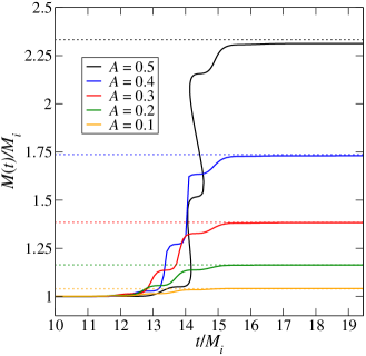
Figure 4: The solid curves are the Christodoulou masses $M(t)$ divided by their initial values $M_{i}$ for the five evolutions with different amplitudes $A=0.1$, 0.2, 0.3, 0.4, and 0.5 for the ingoing pulse of gravitational waves. The horizontal dotted lines denote the ADM energy of each data set, $E_{\text{ADM}}/M_{i}$.

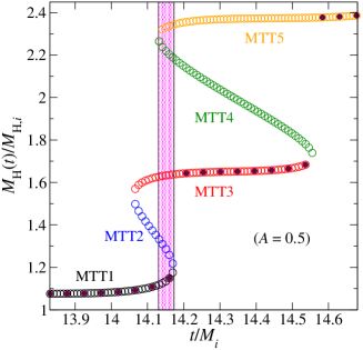
Figure 5: Irreducible mass $M_{\text{H}}$ divided by its initial value $M_{\text{H},i}$ for the evolution with $A=0.5$. The solid circles are the values of $M_{\text{H}}$ for MOTSs found during the evolution. The completed curve is traced out by open circles. The vertical shaded region indicates when five MOTSs exist at the same time.

We now discuss the MOTSs that occur during the five evolutions of the distorted black hole, with amplitude $A=0.1$, 0.2, 0.3, 0.4, or 0.5 for the ingoing gravitational wave pulse. The MOTSs we find are indicated in Fig. 4 by their Christodoulou masses $M$. Early in each simulation, $M$ is approximately constant, and begins to increase when the gravitational wave hits the black hole around $t\approx 12M_{i}$. The effect is more pronounced for larger $A$. The horizontal dotted lines in Fig. 4 indicate the ADM energy of the initial data. Although we do not explicitly calculate the energy carried away by gravitational waves, we can still see that the final Christodoulou mass is close to $E_{\rm ADM}$, indicating that the energy in the gravitational wave pulse predominantly falls into the black hole, and only a small fraction of this energy propagates to null infinity. Even for the highest amplitude case of $A=0.5$, the final value of $M$ is about $99.1\%$ of the ADM energy. These results are as expected. However, for both $A=0.4$ and $A=0.5$, a very interesting new feature arises: multiple concentric MOTSs are present at the same coordinate time.

The evolution with $A=0.5$ shows the multiple MOTSs more distinctly, hence we will focus on it in the remainder of this paper. Figure 5 presents a closer look at the irreducible masses $M_{\text{H}}$ for this case. Locating all MOTSs shown in Fig. 5 requires considerable care. The starting point was the output of the MOTS finder that was run during the evolution, using Gundlach’s fast flow algorithm Gundlach (1998). Because of the computational expense involved, the MOTS finder was not run very frequently, resulting in the solid circles in Fig. 5. The MOTS at the previous time was used as the initial guess for the current time, resulting in a series of MOTSs which is as continuous as possible. The curve traced out by these points has sharp jumps, which was the first indication of the presence of multiple MOTSs at these times. Then to find the remainder of MTT3 and MTT5, an MOTS corresponding to one of these solid circles on MTT3 or MTT5 was used as an initial guess and the MOTS finder was also run more frequently. At this stage, we had completely traced out MTT1, MTT3, and MTT5. Next we found MTT2 and MTT4 to be unstable fixed points for Gundlach’s algorithm, so it was necessary to use our older MOTS finder based on a minimization technique Baumgarte et al. (1996); Pfeiffer et al. (2000, 2002) to find these MTTs. As an initial guess for finding an MOTS on MTT2 for instance, a sphere with radius equal to the average radii of MTT1 and MTT3 sufficed. Once an MOTS on MTT2 was located, it was used as an initial guess for the MOTS finder to locate the MOTSs on neighboring time slices (both later and earlier). The same procedure was used to locate MTT4.

After finding all the MTTs in Fig. 5, a clearer picture of their structures in relation to each other emerged. MTT1 corresponds to the surface of the initial black hole. Shortly after $t=14M_{i}$, a new MOTS with $M_{\text{H}}/M_{\text{H},i}\approx 1.525$ appears and bifurcates into two MTTs. $M_{\text{H}}$ decreases along MTT2, which promptly annihilates with MTT1, while MTT3 persists slightly longer. A similar process then takes place again, and MTT5 is left over as the surface of the final black hole, with $M_{\text{H}}$ more than double its initial value. The vertical shaded region indicates the time interval when five MTTs exist simultaneously. Notice that $M_{\text{H}}$ of the apparent horizon jumps discontinuously in time from the curve of MTT1 to MTT3, and then to MTT5. This indicates that the apparent horizon itself is discontinuous across these times.

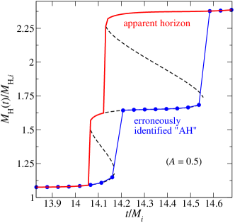
Figure 6: The solid red line denotes the apparent horizon for the evolution with $A=0.5$. The solid blue circles denote an erroneous “apparent horizon,” which is found when the apparent horizon finder is run during the evolution in larger time intervals. The black dashed lines denotes all five MTTs as shown in Fig. 5.

The apparent horizon is the outermost MOTS, and when only one MOTS is present in a black hole evolution, the MOTS and apparent horizon are identical. Here this is not the case, and Fig. 6 shows the apparent horizon in relation to the various MTTs. This figure also highlights another potential pitfall when locating MOTSs. MOTS finders are typically run during the evolution fairly infrequently, using the MOTS from the last MOTS computation as an initial guess (to minimize computational cost). If this had been done for the $A=0.5$ case shown in Figs. 5 and 6, the solid blue circles would have been obtained. Because the previously found MOTS is used as an initial guess, newly appearing MOTSs are generally missed. For instance, the solid blue circles follow MTT1 until it disappears, instead of jumping to MTT3. Therefore, the output of the “apparent horizon finder” (the more widely used name, but technically less precise than “MOTS finder”), is sometimes not the apparent horizon.

A measure of the distortion of the black hole is provided by the intrinsic scalar curvature $\bar{R}$ of the MOTSs. The extrema of $\bar{R}$ is shown in Fig. 7, along with those of the initial apparent horizon. It is interesting to point out that around $t=14.25M_{i}$, the distortion caused by the gravitational waves with $A=0.5$ is sufficiently strong to produce regions of negative $\bar{R}$.

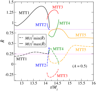
Figure 7: Extrema of the intrinsic scalar curvature $\bar{R}$ of MOTSs during the evolution with $A=0.5$. The horizontal dotted lines are the values for the apparent horizon in the initial data. Around $t=14.25M_{i}$, the MOTSs have regions of negative $\bar{R}$.

V.3 Dynamical Horizons

We determine the signatures of the multiple MTTs during the highly dynamical period. First we compute $\theta_{(k)}$ and $\mathcal{L}_{k}\theta_{(l)}$ using the null normals in Eq. (29), and find that both quantities are negative. So our MTTs are future outer trapping horizons, which must be either spacelike or null, and we can immediately rule out the possibility of there being sections of mixed signatures. Figure 8 shows the extrema of $\theta_{(k)}$ along each MTT. The quantity ${\cal L}_{k}\theta_{(l)}$ is evaluated from the expression Booth and Fairhurst (2007)

$${\cal L}_{k}\theta_{(l)}=-\bar{R}/2+\omega_{\mu}\omega^{\mu}-d_{\mu}\omega^{\mu}+8\pi T_{\mu\nu}l^{\mu}k^{\nu},$$ (38)

where

$$\omega_{\mu}=-\bar{q}^{\nu}_{\mu}k_{\lambda}\nabla_{\nu}l^{\lambda}$$ (39)

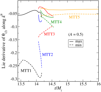
Figure 9: Extrema of ${\cal L}_{k}\theta_{(l)}$ on each MOTS along the MTTs during the evolution with $A=0.5$. For the time shown, ${\cal L}_{k}\theta_{(l)}<0$.

is the normal fundamental form, and $d_{\mu}$ is the covariant derivative compatible with $\bar{q}_{\mu\nu}$. Figure 9 shows the extrema of ${\cal L}_{k}\theta_{(l)}<0$ along each MTT.

Next we compute ${\cal L}_{l}\theta_{(l)}$ to determine whether the MTTs are spacelike or null. We evaluate this using the null Raychaudhuri equation Poisson (2004),

$${\cal L}_{l}\theta_{(l)}=-\sigma^{(l)\mu\nu}\sigma^{(l)}_{\mu\nu}-8\pi T_{\mu\nu}l^{\mu}l^{\nu}.$$ (40)

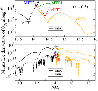
Figure 10: Extrema of $-{\cal L}_{l}\theta_{(l)}$ on each MOTS along the MTTs during the evolution with $A=0.5$. Near $t=14M_{i}$, ${\cal L}_{l}\theta_{(l)}\neq 0$ somewhere on $\mathcal{S}_{v}$.

Figure 10 shows that during the times when there are multiple MTTs, ${\cal L}_{l}\theta_{(l)}\neq 0$ somewhere on each MOTS. Thus all of the MTTs are dynamical horizons at these times.

Here we also mention the extremality parameter $e$ of a MTT introduced in Booth and Fairhurst (2008). In vacuum, it is given by

$$e =\frac{1}{4\pi}\int_{\mathcal{S}}\!\omega_{\mu}\omega^{\mu}\,\sqrt{\bar{q}}d^{2}x,$$ (41)

$$=1+\frac{1}{4\pi}\int_{\mathcal{S}}\!\mathcal{L}_{k}\theta_{(l)}\,\sqrt{\bar{q}}d^{2}x,$$ (42)

where the integral is over an MOTS $\mathcal{S}$ that foliates the MTT. When $\mathcal{S}$ is axisymmetric, this can be regarded as the sum of the squares of all angular momentum multipoles. Because a future outer trapping horizon, which is either spacelike or null, has $\mathcal{L}_{k}\theta_{(l)}<0$, it is always subextremal ($e<1$). So a timelike membrane foliated by future MOTSs (with $\theta_{(k)}<0$) must have $\mathcal{L}_{k}\theta_{(l)}>0$, and is superextremal ($e>1$). Therefore, it was suggested in Booth and Fairhurst (2008) that an MTT’s transition from being spacelike to timelike can be detected when $e\rightarrow 1$.

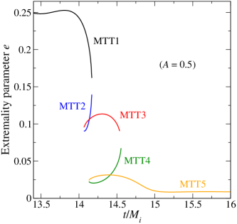
Figure 11: Extremality parameter $e$ along the MTTs during the evolution with $A=0.5$. For the time shown, the MTTs are subextremal with $e<1$, indicating that the MTTs have no timelike sections.

Figure 11 shows $e$ along each MTT, and we see that nowhere does $e\rightarrow 1$, confirming that our MTTs do not become timelike. The value of $e$ shows a substantial decrease after the distortion has left, which is not due to a loss of quasilocal angular momentum $J$ (defined in Eq. (48)), but to the large gain in irreducible mass $M_{\text{H}}$. It may seem that $e$ in Fig. 11 is already rather small to start out with, but one must recall that $e$ depends on the scaling of the null normals $l^{\mu}$ and $k^{\mu}$. That is, we can define new null normals $\bar{l}^{\mu}=fl^{\mu}$ and $\bar{k}^{\mu}=k^{\mu}/f$, rescaled by some function $f$ such that the normalization $\bar{l}^{\mu}\bar{k}_{\mu}=-1$ is preserved. Then $e$ will change as

$$\bar{e}=e+\frac{1}{4\pi}\int_{\mathcal{S}}\!\left[2\omega^{\mu}d_{\mu}\text{ln}f+(d_{\mu}\text{ln}f)(d^{\mu}\text{ln}f)\right]\,\sqrt{\bar{q}}d^{2}x.$$ (43)

Nevertheless, the extremality classification of the MTTs is invariant.

It is known that the irreducible mass $M_{\text{H}}$ of an MOTS must increase along a dynamical horizon Ashtekar and Krishnan (2003), so at first it may seem surprising that MTT2 and MTT4, with decreasing $M_{\text{H}}$ during the evolution, are also dynamical horizons. However, all these MTTs can be viewed as sections of a single dynamical horizon $\mathcal{H}$ that weaves forwards and backwards in time. Then it is clear that the tangent vector to $\mathcal{H}$ along MTT2 and MTT4 points backwards in time, so that $M_{\text{H}}$ is actually increasing along $\mathcal{H}$ as expected. Our simple choice of holding the gauge source function $H_{\mu}$ equal to its initial value leads to a spacetime foliation that interweaves $\mathcal{H}$. This could be avoided by an alternative choice of $H_{\mu}$ that results in a single dynamical horizon that only grows in time.

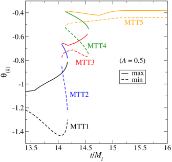
Figure 8: Extrema of $\theta_{(k)}$ on each MOTS along the MTTs during the evolution with $A=0.5$. For the time shown, $\theta_{(k)}<0$.

The situation here resembles an example of a Tolman-Bondi spacetime considered in Booth et al. (2006), where multiple spherically symmetric dust shells fall into a black hole. For their chosen matter distribution, multiple MTTs also formed (up to three at the same time), which were either completely spacelike, or null when the matter density vanished between successive dust shells. In our case the role of the matter density is replaced by the shear $\sigma^{(l)}_{\mu\nu}$ due to the gravitational waves. Since this is always nonvanishing somewhere on the multiple MTTs that form, we only have dynamical horizons.

In Ashtekar and Galloway (2005), it was shown that for a regular dynamical horizon (which is achronal and also a future outer trapping horizon), no weakly trapped surface (on which $\theta_{(l)}\leq 0$ and $\theta_{(k)}\leq 0$) can exist in its past domain of dependence. This helps to explain the difficulty in locating MOTSs along MTT2 and MTT4 using flow methods. For example, consider locating an MOTS on MTT2 at $t=14.1M_{i}$ shown in Fig. 5. If we use a trial surface $\mathcal{S}$ located between the MOTSs on MTT1 and MTT2, it must have $\theta_{(l)}>0$ because it lies in the past domain of dependence of $\mathcal{H}$. This means that $\mathcal{S}$ will be moved inwards when using flow methods, away from MTT2. If we switch to having $\mathcal{S}$ lie between the MOTSs on MTT2 and MTT3, then having $\theta_{(l)}>0$ is desired. Unfortunately, now $\mathcal{S}$ lies in the future domain of dependence of $\mathcal{H}$, and we are no longer guaranteed that $\mathcal{S}$ is not a weakly trapped surface.

V.4 Dynamical Horizon Flux Law

The growth of a black hole in full, nonlinear general relativity can be described by the dynamical horizon flux law of Ashtekar and Krishnan Ashtekar and Krishnan (2002, 2003), which relates the increase in area or mass along a dynamical horizon to fluxes of matter and gravitational energy across it. Here, we will evaluate this flux law for the dynamical horizon $\mathcal{H}$ that consists of the multiple MTT sections we found earlier, using the form given in Booth and Fairhurst (2007).

To state the dynamical horizon flux law, let us specifically consider the change in the irreducible mass $M_{\text{H}}$ along $\mathcal{H}$. Denote an MOTS that foliates $\mathcal{H}$ by $\mathcal{S}_{v}$, which is labeled by a foliation parameter $v$ that is constant on $\mathcal{S}_{v}$. Then choose a tangent vector $V^{\mu}$ to $\mathcal{H}$ that is normal to each $\mathcal{S}_{v}$, and such that

$${\cal L}_{V}v=1.$$ (44)

This vector $V^{\mu}$ can be written as

$$V^{\mu}=\bar{B}\bar{l}^{\mu}-\bar{C}\bar{k}^{\mu},$$ (45)

in terms of coefficients $\bar{B}$ and $\bar{C}$, and null normals $\bar{l}^{\mu}=fl^{\mu}$ and $\bar{k}^{\mu}=k^{\mu}/f$ that are rescaled by a function $f$ (but still having $\bar{l}^{\mu}\bar{k}_{\mu}=-1$) so that

$$\bar{C}=2\frac{dM_{\text{H}}}{dv}.$$ (46)

The dynamical horizon flux law is then

$$\frac{dM_{\text{H}}}{dv}=\int_{\mathcal{S}_{v}}\!\left[T_{\mu\nu}\bar{l}^{\mu}\tau^{\nu}+\frac{\bar{B}}{8\pi}\sigma^{(\bar{l})}_{\mu\nu}\sigma^{(\bar{l})\mu\nu}+\frac{\bar{C}}{8\pi}\bar{\omega}_{\mu}\bar{\omega}^{\mu}\right]\,\sqrt{\bar{q}}d^{2}x,$$ (47)

where $\sigma^{(\bar{l})}_{\mu\nu}$ and $\bar{\omega}_{\mu}$ are given by Eqs. (34) and (39) but in terms of $\bar{l}^{\mu}$ and $\bar{k}^{\mu}$, and $\tau^{\mu}=\bar{B}\bar{l}^{\mu}+\bar{C}\bar{k}^{\mu}$ is the normal vector to $\mathcal{H}$.

The first term in Eq. (47) involving $T_{\mu\nu}$ is the energy flux of matter across $\mathcal{S}_{v}$, and the second term involving $\sigma^{(\bar{l})}_{\mu\nu}$ is a flux of gravitational energy Ashtekar and Krishnan (2003). The last term has been interpreted differently by various authors. The normal fundamental form $\omega_{\mu}$ (or $\bar{\omega}_{\mu}$) enters into the definition of the quasilocal angular momentum $J$ of a black hole mentioned at the end of Sec. II, which is given by Ashtekar and Krishnan (2003),

$$J=-\frac{1}{8\pi}\int_{\mathcal{S}_{v}}\!\phi^{\mu}\omega_{\mu}\,\sqrt{\bar{q}}d^{2}x,$$ (48)

for any choice of rotation vector field $\phi^{\mu}$ on $\mathcal{S}_{v}$. Because of this relation, this term has been interpreted as a flux of rotational energy Ashtekar and Krishnan (2003); Schnetter et al. (2006). However, it has been pointed out in Booth and Fairhurst (2007) that this is unlikely, as $\omega_{\mu}$ is related to $J$ itself and not its flux. Indeed, this may be illustrated by considering a Kerr black hole that is distorted by an ingoing spherically symmetric dust shell (which carries no angular momentum). So even though there will be no flux of rotational energy, the last term in Eq. (47) will still be nonzero whenever $\bar{C}\neq 0$, which is necessarily true on a dynamical horizon. This last term also closely resembles the extremality parameter $e$ mentioned in Sec. V.3.

Another interpretation of the last term in Eq. (47) has been given by Hayward Hayward (2006) as a flux of longitudinal gravitational radiation, by examining the components of an effective gravitational radiation energy tensor in spin-coefficient form. At future null infinity, the outgoing longitudinal gravitational radiation is negligible relative to the outgoing transverse radiation, but near the black hole this is generally not so.

To evaluate the dynamical horizon flux law, we first construct a tangent vector $X^{\mu}$ to $\mathcal{H}$ that connects $\mathcal{S}_{v}$ in $\Sigma_{t}$ to $\mathcal{S}_{v^{\prime}>v}$ in $\Sigma_{t^{\prime}}$ as

$$X^{\mu}=\pm\left(1,\frac{\partial x^{i}_{v}}{\partial t}\right),$$ (49)

where $x^{i}_{v}$ are the coordinates of $\mathcal{S}_{v}$, and the plus sign is for $t^{\prime}>t$ while the minus sign is for $t^{\prime}<t$. The latter occurs along MTT2 and MTT4. The spatial components of the tangent vector $X^{\mu}$ diverge when two MTT sections meet. This may be avoided by a different choice of $X^{\mu}$, but here we employ the simple one described above. For this reason, we also consider the corresponding foliation parameter $v$ along each section of $\mathcal{H}$ separately. Since

$${\cal L}_{X}v=\pm\frac{\partial v}{\partial t},$$ (50)

and we would like this to be unity, it follows that $v=\pm t+v_{0}$, where $v_{0}$ is some constant along each MTT section. We choose $v=t$ along MTT1. Along the other MTT sections, we choose $v_{0}$ so that $v=0$ on the first $\mathcal{S}_{v}$ we find on those sections.

Next we make $X^{\mu}$ orthogonal to $\mathcal{S}_{v}$ to obtain $V^{\mu}$ (while leaving the time component unchanged, so Eq. (44) is still satisfied with the choice of $v$ described above). To achieve this, we use the unit tangent vectors to $\mathcal{S}_{v}$,

$$p^{\mu}=N_{p}\left(0,\frac{\partial x^{i}_{v}}{\partial\theta}\right)\hskip 5.69054pt\text{and}\hskip 5.69054ptq^{\mu}=N_{q}\left(0,\frac{1}{\sin\theta}\frac{\partial x^{i}_{v}}{\partial\phi}\right).$$ (51)

Here, $x^{i}_{v}(\theta,\phi)=c^{i}_{\rm MOTS}+r_{\rm MOTS}(\theta,\phi)d^{i}(\theta,\phi)$ where $r_{\rm MOTS}(\theta,\phi)$ is given in Eq. (36) and $d^{i}$ is the coordinate unit vector pointing from the origin $c^{i}_{\rm MOTS}$ of the expansion along the $(\theta,\phi)$-directions. Also, $N_{p}$ and $N_{q}$ are normalization factors such that $p^{2}=q^{2}=1$. Orthogonalizing $q^{\mu}$ against $p^{\mu}$ gives the vector

$$Q^{\mu}=N_{Q}\left(q^{\mu}-p^{\nu}q_{\nu}p^{\mu}\right),$$ (52)

where $N_{Q}$ is again a normalization factor such that $Q^{2}=1$. Then we obtain the desired tangent vector to $\mathcal{H}$ as

$$V^{\mu} =X^{\mu}-\left(p^{\nu}X_{\nu}\right)p^{\mu}-\left(Q^{\nu}X_{\nu}\right)Q^{\mu}.$$ (53)

This can be also be expressed in terms of our standard null normals of Eq. (29) as

$$V^{\mu}=Bl^{\mu}-Ck^{\mu},$$ (54)

with coefficients $B=-V^{\mu}k_{\mu}$ and $C=V^{\mu}l_{\mu}$.

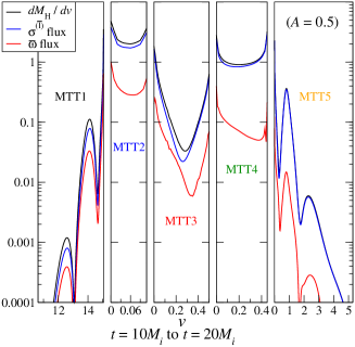
Figure 12: Terms in the dynamical horizon flux law of Eq. (47) plotted against the foliation parameter $v$ along each section of $\mathcal{S}_{v}$. Along MTT1, we choose $v=t$. Along the other MTT sections, we choose $v=0$ on the first $\mathcal{S}_{v}$ we find.

Now we determine the rescaled null normals $\bar{l}^{\mu}$ and $\bar{k}^{\mu}$ appearing in Eq. (45). Since $V^{\mu}$ must be the same vector whether it is written in terms of $l^{\mu}$ and $k^{\mu}$, or $\bar{l}^{\mu}$ and $\bar{k}^{\mu}$, we have the relations

$$\bar{B}=B/f\hskip 5.69054pt\text{and}\hskip 5.69054pt\bar{C}=fC,$$ (55)

which together with Eq. (46) gives

$$\ f=\frac{B}{\bar{B}}=\frac{\bar{C}}{C}=\frac{2}{C}\frac{dM_{\text{H}}}{dv}.$$ (56)

Evaluating the scale factor $f$ requires knowledge of $dM_{\text{H}}/dv$. It is straightforward to show that the area element $\sqrt{\bar{q}}$ of $\mathcal{S}_{v}$ changes along $\mathcal{H}$ as

$${\cal L}_{V}\sqrt{\bar{q}}=-C\theta_{(k)}\sqrt{\bar{q}},$$ (57)

so the change in the cross-sectional area $A_{\text{H}}$ along $\mathcal{H}$ is

$$\frac{dA_{\text{H}}}{dv}=-\int_{\mathcal{S}_{v}}\!C\theta_{(k)}\,\sqrt{\bar{q}}d^{2}x.$$ (58)

From the definition $M_{\text{H}}=\sqrt{A_{\text{H}}/{16{\pi}}}$, it then follows that

$$\frac{dM_{\text{H}}}{dv}=\frac{1}{\sqrt{64\pi A_{\text{H}}}}\frac{dA_{\text{H}}}{dv}.$$ (59)

The terms in the dynamical horizon flux law (47) are calculated by noting that under the rescaling of the null normals $l^{\mu}$ and $k^{\mu}$,

$$\sigma^{(\bar{l})}_{\mu\nu}=f\sigma^{(l)}_{\mu\nu}\hskip 5.69054pt\text{and}\hskip 5.69054pt\bar{\omega}_{\mu}=\omega_{\mu}+d_{\mu}\ln f.$$ (60)

The results are shown in Fig. 12 from $t=10M_{i}$ to $t=20M_{i}$. The energy flux of matter is neglected since we have $T_{\mu\nu}=0$. The flux associated with $\bar{B}\sigma^{(\bar{l})}_{\mu\nu}\sigma^{(\bar{l})\mu\nu}$, labeled as “$\sigma^{(\bar{l})}$ flux”, is always the larger contribution to the growth of $M_{\text{H}}$, which is expected from the interpretation of this term as a flux of gravitational energy. This is most pronounced along MTT2 and MTT4, with decreasing $M_{\text{H}}$ during the evolution, and clearly indicates that their appearance is a consequence of the sufficiently high gravitational energy flux across them. We have seen in Sec. V.2 that for weak gravitational waves and with the same gauge condition for the evolution, no such MTTs appear. The maximum number of MTTs that can exist at the same time may also be linked to the structure of the gravitational waves, as shown in the inset of Fig. 2, although we have not explored this aspect further.

The fluxes increase rapidly near each bifurcation point. This is because of our choice of normalization for $X^{\mu}$ in Eq. (49), which propagates into $V^{\mu}$. To understand this, let us write as $x^{\mu}_{c}$ the spacetime coordinates of $\mathcal{S}_{c}$ that bifurcates, with foliation parameter $v=c$ say. Then on a nearby $\mathcal{S}_{v}$, we can approximate $\partial x^{i}_{v}/\partial t$ by

$$\frac{\partial x^{i}_{v}}{\partial t}\approx\frac{\partial}{\partial t}\left(x^{i}_{c}\pm\lambda\sqrt{|t-t_{c}}|\right)=\pm\frac{\lambda}{2}\frac{1}{\sqrt{|t-t_{c}|}},$$ (61)

where $\lambda$ is some function. As $t\rightarrow t_{c}$, this quantity diverges as does the norm of $V^{\mu}$, and leads to the higher values of the fluxes measured along $V^{\mu}$. This singular behavior could be absorbed into a redefined foliation parameter $v^{\prime}=v^{\prime}(v)$. Also, any visible discontinuities in the fluxes across different sections of $\mathcal{H}$ in Fig. 12 are due to the difficulty in finding $\mathcal{S}_{c}$ exactly (as indicated by the data points in Fig. 5, even searching for MOTSs at every $\Delta t=0.01$ is insufficient for this purpose).

V.5 Angular Momentum Flux Law

The angular momentum $J$ defined in Eq. (48) depends on a choice of rotation vector $\phi^{\mu}$ on $\mathcal{S}_{v}$. If $\mathcal{S}_{v}$ is axisymmetric, the natural choice of $\phi^{\mu}$ is the axial Killing vector. In general spacetimes no such Killing vector exists, but one can nevertheless define a suitable $\phi^{\mu}$ Booth and Fairhurst (2005) by requiring it to have closed orbits, and be divergence-free

$$d_{\mu}\phi^{\mu}=0.$$ (62)

This notion has been further refined to calculate approximate Killing vectors Lovelace et al. (2008); Cook and Whiting (2007) in black hole simulations, and we will make use of this choice here. They were also used to compute $J$ of the initial data sets in Sec. II.

Gourgoulhon has generalized the Damour-Navier-Stokes equation for null hypersurfaces to trapping horizons and used it to derive a flux law for the change in $J$ along a hypersurface $\mathcal{H}$ foliated by 2-surfaces $\mathcal{S}_{v}$ (not necessarily MOTSs) with foliation parameter $v$ Gourgoulhon (2005),

$$\frac{dJ}{dv}= -\int_{\mathcal{S}_{v}}\!T_{\mu\nu}\phi^{\mu}\tau^{\nu}\,\sqrt{\bar{q}}d^{2}x$$ (63)

$$-\frac{1}{16\pi}\int_{\mathcal{S}_{v}}\!\sigma^{(\tau)\mu\nu}{\cal L}_{\phi}\bar{q}_{\mu\nu}\,\sqrt{\bar{q}}d^{2}x$$

$$+\int_{\mathcal{S}_{v}}\!\frac{1}{8\pi}\left[\theta_{(k)}\phi^{\mu}d_{\mu}C-\omega_{\mu}{\cal L}_{V}\phi^{\mu}\right]\,\sqrt{\bar{q}}d^{2}x$$

$$= -\int_{\mathcal{S}_{v}}\!T_{\mu\nu}\phi^{\mu}\tau^{\nu}\,\sqrt{\bar{q}}d^{2}x$$ (64)

$$-\int_{\mathcal{S}_{v}}\frac{1}{8\pi}\left[B\sigma^{(l)}_{\mu\nu}\sigma^{(\phi)\mu\nu}+C\sigma^{(k)}_{\mu\nu}\sigma^{(\phi)\mu\nu}\right]\,\sqrt{\bar{q}}d^{2}x$$

$$+\int_{\mathcal{S}_{v}}\!\frac{1}{8\pi}\left[\theta_{(k)}\phi^{\mu}d_{\mu}C-\omega_{\mu}{\cal L}_{V}\phi^{\mu}\right]\,\sqrt{\bar{q}}d^{2}x,$$

where the vectors $V^{\mu}=Bl^{\mu}-Ck^{\mu}$ and $\tau^{\mu}=Bl^{\mu}+Ck^{\mu}$ are tangent and normal to $\mathcal{H}$, respectively. The first integral in Eq. (64) is the angular momentum flux due to matter. The second integral can be thought of as the flux due to gravitational radiation and vanishes if $\mathcal{S}_{v}$ is axisymmetric. In addition, it is usually required that $\phi^{\mu}$ be Lie transported along the dynamical horizon,

$$\mathcal{L}_{V}\phi^{\mu}=0,$$ (65)

so that the last integral in Eq. (64) vanishes when $\mathcal{S}_{v}$ is an MOTS Gourgoulhon (2005). This requirement ensures that in the absence of matter and gravitational radiation, the angular momentum flux will be zero along an MTT as expected, instead of there being some physically unmeaningful flux simply due to measuring $J$ about different axes.

Here we evaluate the angular momentum flux law for the dynamical horizon $\mathcal{H}$ found in Sec. V.3 for $A=0.5$. Because we calculate $J$ with $\phi^{\mu}$ being an approximate Killing vector, Eq. (65) is not satisfied in general, and so we must keep the last integral in Eq. (64). We use the same tangent vector $V^{\mu}$ and foliation parameter $v$ along each section of $\mathcal{H}$ as in Sec. V.4, and the null normals to $\mathcal{S}_{v}$ given in Eq. (29). The values of the terms in Eq. (64) are shown in Fig. 13 from $t=10M_{i}$ to $t=20M_{i}$. The first integral is neglected since $T_{\mu\nu}=0$. The two terms in the second integral are labeled as “$B\sigma^{(l)}\sigma^{(\phi)}$ flux” and “$C\sigma^{(k)}\sigma^{(\phi)}$ flux”. The last integral is labeled as “$\mathcal{L}_{V}\phi^{\mu}$ flux”. The angular momentum flux $dJ/dv$ is dominated by the flux associated with $B\sigma^{(l)}_{\mu\nu}\sigma^{(\phi)\mu\nu}$, due to the large $\sigma^{(l)}_{\mu\nu}$ produced by the gravitational waves. The magnitude of $dJ/dv$ vanishes initially, becomes largest along the end of MTT1 and the beginning of MTT2 when the gravitational waves reach the black hole, and settles back down to zero again along the successive MTT sections. Because $dJ/dv$ alternates sign along $\mathcal{H}$, the net change in $J$ turns out to be small. The terms in the angular momentum flux law also diverge near each $\mathcal{S}_{v}$ that bifurcates into two MTTs, just like the terms in the dynamical horizon flux law in Fig. 12, and again is a consequence of our choice of $V^{\mu}$ as discussed at the end of Sec. V.4.

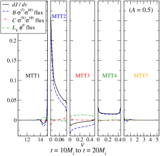
Figure 13: Terms in the angular momentum flux law of Eq. (64) plotted against the foliation parameter $v$ along each section of $\mathcal{H}$. Along MTT1, we choose $v=t$. Along the other MTT sections, we choose $v=0$ on the first $\mathcal{S}_{v}$ we find.

VI The Event Horizon

VI.1 Basic Definitions and Concepts

The standard definition of the surface of a black hole is the event horizon, the boundary of the set of all points that are not in the causal past of future null infinity Wald (1984). It is a null hypersurface, generated by null geodesics that have no future endpoints. As defined, the event horizon is a 3-surface, but it is common to refer to the intersection of this surface with $\Sigma_{t}$ as the event horizon as well. In contrast to an MOTS, the event horizon can only be found after the entire future history of the spacetime is known. Because of its teleological nature, the event horizon can behave nonintuitively. For instance, before a gravitational collapse has occurred an event horizon already forms, even though there is no flux of energy or angular momentum across it yet. In this section we describe our method of finding the event horizon, and contrast its properties with those of the MTTs found in Sec. V.

VI.2 Event Horizon Finder

The event horizon is located in a spacetime by following geodesics backward in time. It is well known Anninos et al. (1995); Libson et al. (1996) that null outgoing geodesics in the vicinity of the event horizon, when followed backwards in time, will converge onto the event horizon exponentially. Therefore, given a well-chosen congruence of geodesics, one can trace the event horizon of the spacetime with exponentially (in time) improving accuracy.

Our event horizon finder Cohen et al. (2009) tracks a set of geodesics backwards in time. The initial guess for the event horizon is chosen at some late time when the black hole is in a quasistationary state. At this time, the apparent horizon and event horizon coincide closely, and the apparent horizon is used as the initial guess. The initial direction of the geodesics is chosen to be normal to the apparent horizon surface, and the geodesics are integrated backwards in time. The geodesic equation requires values for the metric and its derivatives for each geodesic at each point in time. These values are obtained by interpolation from the values computed during the evolution. With an appropriate form of the geodesic equation, we can follow a geodesic as a function of coordinate time $t$, rather than the affine parameter along the geodesic.

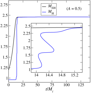
Figure 14: Irreducible masses of the event horizon $M_{\text{EH}}$ and the MOTSs $M_{\text{H}}$ during the evolution with $A=0.5$. At the very beginning of the evolution $M_{\text{EH}}$ is already increasing, while $M_{\text{H}}$ is still fairly constant. As the inset shows, $M_{\text{EH}}$ grows very slightly when $M_{\text{H}}$ changes the most.

VI.3 Contrasting the Event Horizon with MTTs

We find the event horizon for the evolution in which the ingoing gravitational waves have the largest amplitude $A=0.5$. The surface area $A_{\text{EH}}$ of the event horizon is computed by integrating the metric induced on its surface by the spatial metric $g_{ij}$. The irreducible mass of the event horizon is then given as $M_{\text{EH}}=\sqrt{A_{\text{EH}}/16\pi}$. This is shown in Fig. 14, together with the irreducible mass $M_{\text{H}}$ along the MTTs. An obvious difference is that $M_{\text{EH}}$ always increases in time, and the event horizon does not bifurcate like the MTTs shortly after $t=14M_{i}$. The event horizon is also already growing at the very beginning of the evolution, before the gravitational waves have hit the black hole. By $t=14M_{i}$, the value of $M_{\text{EH}}$ has almost doubled while $M_{\text{H}}$ is still fairly close to its initial value. In fact, during the time when multiple MTTs are present and one would intuitively expect the black hole to be the most distorted, the event horizon shows very little growth.

This peculiar behavior of the event horizon was also illustrated in Booth (2005) for the gravitational collapse of spherical dust shells, and explained with the null Raychaudhuri equation Poisson (2004),

$$\frac{d\theta_{(l)}}{d\lambda}=-\frac{1}{2}\theta_{(l)}^{2}-\sigma^{(l)}_{\mu\nu}\sigma^{(l)\mu\nu}-8\pi T_{\mu\nu}l^{\mu}l^{\nu},$$ (66)

where $\lambda$ is an affine parameter along the congruence of null geodesics that generate the event horizon, with tangent vector $l^{\mu}$. The area element $\sqrt{h}$ of the event horizon is related to the expansion $\theta_{(l)}$ by $d\sqrt{h}/d\lambda=\theta_{(l)}\sqrt{h}$, and substituting this into Eq. (66) gives

$$\frac{d^{2}\sqrt{h}}{d\lambda^{2}}=\left(\frac{1}{2}\theta_{(l)}^{2}-\sigma^{(l)}_{\mu\nu}\sigma^{(l)\mu\nu}-8\pi T_{\mu\nu}l^{\mu}l^{\nu}\right)\sqrt{h}.$$ (67)

In dynamical situations we will generally have $\theta_{(l)}\neq 0$ on the event horizon, and this accounts for its accelerated growth, which is evident even at early times in our evolution when the shear $\sigma^{(l)}_{\mu\nu}$ is negligible. When the pulse of gravitational waves hits the black hole, $\sigma^{(l)}_{\mu\nu}$ on the event horizon becomes large, and according to Eq. (67) this will decelerate its growth, even causing the growth to become very small in our case.

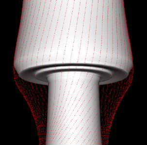
Figure 15: Spacetime diagram of the event horizon and dynamical horizons for $A=0.5$. The dotted red lines are the null generators of the event horizon, while the solid grey surface represents the dynamical horizons.

At late times, the event and apparent horizons eventually coincide as both $\sigma^{(l)}_{\mu\nu}$ and $\theta_{(l)}$ go to zero on the event horizon while the apparent horizon becomes null. Finally, Fig. 15 shows a spacetime diagram of the event horizon and the dynamical horizon $\mathcal{H}$, with the spatial dimension along the $z-$direction suppressed. The null generators of the event horizon are shown as dotted red lines, and lie outside the solid grey surface of $\mathcal{H}$, except when they coincide at late times. In Fig. 15 the event horizon’s cross section appears to be shrinking at late times. The constancy of the area of the event horizon (cf. Fig. 14) shows that this is merely a coordinate effect.

VII Discussion

In this paper, we investigate marginally trapped tubes and the event horizon for rotating black holes distorted by a pulse of ingoing gravitational waves. For small distortions (low amplitude $A$), the simulations do not exhibit any unexpected behavior: the area of the apparent horizon is initially approximately constant, it grows when the gravitational radiation reaches the black hole, and then settles down to a constant value after the highly dynamical regime is over. However, for strong distortions, we find much more interesting behaviors of the MOTSs. A new pair of MOTSs appears outside the original MOTS. These new surfaces are initially close together and move rapidly away from each other, indicating that at the critical time when they first appear they are coincident (although this particular event cannot be resolved in an evolution with finite time step). The inner surface of such a pair shrinks, eventually approaches the original MOTS, and then these two surfaces annihilate each other. For amplitude $A=0.4$ this process happens once, for $A=0.5$ this happens twice, and there is a short time interval during which five MOTSs are present in the simulation.

The MTTs traced out by the MOTSs are smooth, and appear to combine into one smooth hypersurface (although the critical points where different marginally trapped tubes combine with each other cannot be resolved). When the black hole is distorted, we find that this hypersurface is everywhere spacelike and a dynamical horizon. We investigate how the black hole grows by evaluating the dynamical horizon flux law of Ashtekar and Krishnan Ashtekar and Krishnan (2003); Booth and Fairhurst (2007), and find that the gravitational energy flux is largest across the sections of the dynamical horizon that decrease in cross-sectional area with increasing time. We also evaluate the angular momentum flux law of Gourgoulhon Gourgoulhon (2005) along the dynamical horizon, but instead of using a rotation vector $\phi^{\mu}$ that is Lie transported along the dynamical horizon, we use an approximate Killing vector Lovelace et al. (2008), since we prefer to calculate the angular momentum itself in this way. The angular momentum flux law is based on the generalized Damour-Navier-Stokes equation, which treats the black hole as a viscous fluid. Evaluating the generalized Damour-Navier-Stokes equation itself could aid in developing physical intuition about black holes in numerical spacetimes.

In illustrating the procedure for finding multiple MOTSs, caution must be taken to locate the apparent horizon with MOTS finders when the MOTS found at a previous time is used as an initial guess. If the MOTS finder is not run frequently enough, new MOTSs will be missed and an erroneous apparent horizon will be identified. This raises the issue of whether the true apparent horizon was indeed located in similar work involving highly distorted black holes in the past (e.g. Anninos et al. (1994)). A better understanding of the slicing dependence of the MOTSs in our simulations would also be helpful in choosing a more natural slicing condition that gives a single dynamical horizon that only grows in the cross-sectional area with time in highly dynamical situations.

When computing the event horizon, we find it to be smooth, and enveloping the complicated structure of the MOTSs. As can be seen in Figs. 14 and 15, the event horizon is very close to the apparent horizon at late times, as one would expect. The motion of the event horizon is restricted by the fact that it is foliated by null geodesics. Therefore, in order to encompass the MOTSs, the event horizon begins to grow much earlier, and even at the start of our simulation the event horizon is already considerably larger than the apparent horizon. At early times, $t\lesssim 10M_{i}$, the event horizon approaches the apparent horizon exponentially. The rate of approach should be given by the surface gravity of the initial black hole, but we have not verified this in detail, as our simulation does not reach sufficiently far into the past. This could be checked by placing the initial pulse of gravitational radiation at a larger distance from the black hole. The growth of the event horizon is described by the Hawking-Hartle formula Hawking and Hartle (1972), which may also be evaluated to give a more complete comparison of MTTs and the event horizon.

Our findings are analogous to the behavior of MOTSs and event horizons in the Vaidya spacetime, as worked out in detail in the Appendix. In particular, for strong accretion, the Vaidya spacetime can also exhibit multiple MOTSs at the same time, all of which foliate dynamical horizons. Both in the Vaidya spacetime and our distorted Kerr spacetimes, the event horizon begins to grow much earlier before multiple MOTSs appear. By choosing a mass functions $m(v)$ that has two strong pulses of accretion, the Vaidya example in the Appendix would also produce five concentric MOTSs similar to that seen in Fig. 5.

Appendix A Multiple Horizons in the Vaidya Spacetime

The ingoing Vaidya spacetime is a spherically symmetric spacetime describing a black hole that accretes null dust Vaidya (1951). It shares similar features to the distorted Kerr spacetimes presented in this paper, which we mention here briefly. The ingoing Vaidya metric in ingoing Eddington-Finkelstein coordinates $(v,r,\theta,\phi)$ is

$$ds^{2}=-\left(1-\frac{2m(v)}{r}\right)dv^{2}+2dvdr+r^{2}d\Omega^{2},$$ (68)

where $v=t+r$ is advanced time (not to be confused with the foliation parameter $v$ of dynamical horizon in the main text). From the Einstein equations, the stress-energy tensor is

$$T_{\mu\nu}=\frac{dm/dv}{4\pi r^{2}}(\partial_{\mu}v)(\partial_{\nu}v).$$ (69)

With the choice of radial outgoing and ingoing null vectors

$$l^{\mu}=\left[1,\frac{1}{2}\left(1-\frac{2m(v)}{r}\right),0,0\right]\hskip 5.69054pt\text{and}\hskip 5.69054ptk^{\mu}=(0,-1,0,0)$$ (70)

normalized so that $l^{\mu}k_{\mu}=-1$, the expansions of the null normals are

$$\theta_{(l)}=\frac{1}{r}\left(1-\frac{2m(v)}{r}\right)\hskip 5.69054pt\text{and}\hskip 5.69054pt\theta_{(k)}=-\frac{2}{r}.$$ (71)

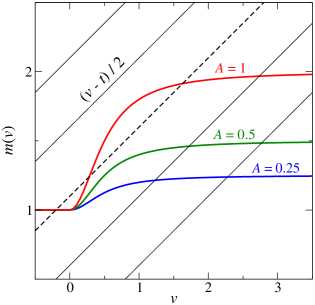
Figure 16: Mass functions $m(v)$ of the Vaidya spacetime for three amplitudes $A=0.25,0.5$, and 1, along with the straight lines $(v-t)/2$. MOTSs exist at the intersections of these functions. For $A=0.5$ and 1, there are up to three intersections, as illustrated by the dashed black line which intersects the $A=1$ mass curve three times.

From this, we see that MOTSs are located at $r=2m(v)$, or

$$m(v)=\frac{1}{2}(v-t).$$ (72)

The number of solutions to Eq. (72), i.e. the number of MOTSs, can be conveniently discussed with the diagram shown in Fig. 16. The thick solid lines represent three different mass functions $m(v)$ plotted vs $v$. The right-hand side of Eq. (72) is a family of straight lines (one for each $t$) represented by the thin diagonal lines in Fig. 16. For a given $t$, the number of intersections between the $(v-t)/2$ and the $m(v)$ curve gives the number of MOTSs at that particular $t$. The straight line $\frac{1}{2}(v-t)$ has slope 1/2, so if $dm/dv<1/2$ for all $v$, then there will be exactly one intersection for every $t$. If

$$\frac{dm}{dv}>\frac{1}{2}\qquad\mbox{for some $v$,}$$ (73)

then the $m(v)$ curve will have regions that are steeper than the straight line. By adjusting the vertical intercept of the straight line, equivalent to choosing a suitable $t$, the straight line will pass through a point with $dm/dv>1/2$. At this point, $m(v)$ passes from below to above the straight line, so there must be an additional intersection at both smaller and larger $v$, for a total of three MOTSs. Thus, sufficiently rapid mass accretion (large $dm/dv$) results in multiple MOTSs.

The signature of a spherically symmetric MTT depends on the sign of Booth et al. (2006)

$$C=\frac{T_{\mu\nu}l^{\mu}l^{\nu}}{1/(2A_{\rm H})-T_{\mu\nu}l^{\mu}k^{\nu}},$$ (74)

where $A_{\rm H}$ is the cross-sectional area of the MTT. The MTT is spacelike if $C>0$, null if $C=0$, and timelike if $C<0$. From Eq. (69) and Eq. (70),

$$T_{\mu\nu}l^{\mu}l^{\nu}=\frac{dm/dv}{4\pi r^{2}}\hskip 5.69054pt\text{and}\hskip 5.69054ptT_{\mu\nu}l^{\mu}k^{\nu}=0,$$ (75)

so we see that $C>0$ for the Vaidya spacetime as long as $dm/dv>0$. Furthermore, since $\theta_{(k)}<0$, these MTTs will also be dynamical horizons.

The event horizon is generated by radial outgoing null geodesics satisfying

$$\frac{dr}{dv}=\frac{1}{2}\left(1-\frac{2m(v)}{r}\right).$$ (76)

Integrating this differential equation requires knowledge of the event horizon location at some point. This is usually supplied by the final state of the black hole, when accretion has ended.

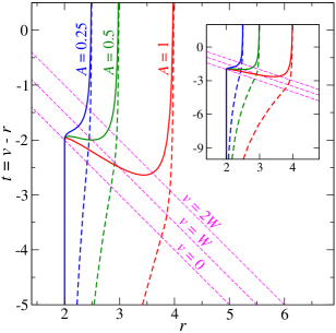
Figure 17: Locations of MOTSs (solid lines) and event horizons (dashed lines) in the Vaidya spacetime. For $A=0.25$ there is one MOTS at all times. For $A=0.5$ and 1, up to three MOTSs exist at a time $t$. The event horizons approach the MTTs at very early and late times, and start growing much earlier than the MTTs. The inset shows a larger interval in $t$.

To close, we illustrate these considerations with a concrete example. We choose the mass function

$$m(v)=\left\{\begin{aligned} &m_{0},&\qquad v\leq 0\\ &m_{0}+\frac{Am_{0}v^{2}}{v^{2}+W^{2}},&\qquad v>0\end{aligned}\right.$$ (77)

similar to that presented in Schnetter and Krishnan (2006) ($Am_{0}$ is the mass accreted by the black hole, and $W$ determines the time scale of accretion). We set $m_{0}=1$, $W=0.5$, and consider three different amplitudes $A=0.25,0.5$, and 1. Figure 16 shows the respective mass functions, and we see that $A=0.25$ never leads to multiple MOTSs, while $A=1$ clearly exhibits three MOTSs for certain $t$. It is easy to show that Eq. (73) implies $Am_{0}>4W/(3\sqrt{3})$. The locations of the MOTSs in $(r,t)$ coordinates are shown in Fig. 17. For $A=0.25$, there is only one MOTS at all times. For $A=0.5$, there are up to three MOTSs at a single time. A new MOTS appears at $r=2.5$ immediately after $t=-2$, and bifurcates into two MTTs. One of these MTTs shrinks and annihilates with the innermost MTT at $t=-1.93256$, while only the outermost MTT remains at late times and grows towards $r=3$. For $A=1$, there are again up to three MOTSs at a single time, but a new MOTS appears earlier at $t=-2.63822$. After $t=-1.96824$, only one MOTS remains and grows towards $r=4$. Also shown in Fig. 17 are lines of constant $v$ indicating when accretion begins ($v=0$), and when $m(v)$ has increased by $50\%$ and $80\%$, respectively ($v=W$ and $v=2W$).

The event horizons for the three cases are computed by integrating Eq. (76) backward in time, starting with $r_{\rm EH}(v\to\infty)=2(1+A)m_{0}$. The resulting surfaces are shown as the dashed curves in Fig. 17. The event horizon is located at $r=2$ in the far past, starts growing long before $m(v)$ increases, and asymptotically approaches the MTT of the final black hole for all amplitudes $A$.

References

- Bernstein et al. (1994) D. Bernstein, D. Hobill, E. Seidel, and L. Smarr, Phys. Rev. D 50, 3760 (1994).
- Thorne (1972) K. S. Thorne, in Magic Without Magic; John Archibald Wheeler, edited by J. Klauder (Frieman, San Francisco, 1972).
- Anninos et al. (1994) P. Anninos, D. Bernstein, S. R. Brandt, D. Hobill, E. Seidel, and L. Smarr, Phys. Rev. D 50, 3801 (1994).
- Brandt and Seidel (1995) S. R. Brandt and E. Seidel, Phys. Rev. D 52, 870 (1995).
- Anninos et al. (1995) P. Anninos, D. Bernstein, S. Brandt, J. Libson, J. Massó, E. Seidel, L. Smarr, W.-M. Suen, and P. Walker, Phys. Rev. Lett. 74, 630 (1995).
- Hawking and Ellis (1973) S. W. Hawking and G. F. R. Ellis, The large scale structure of space-time (Cambridge University Press, Cambridge, England, 1973).
- Wald (1984) R. M. Wald, General Relativity (University of Chicago Press, Chicago and London, 1984).
- Penrose (1965) R. Penrose, Phys. Rev. Lett. 14, 57 (1965).
- Hayward (1994) S. A. Hayward, Phys. Rev. D 49, 6467 (1994).
- Hayward (2004) S. A. Hayward, Phys. Rev. Lett. 93, 251101 (2004).
- Ashtekar et al. (2000a) A. Ashtekar, C. Beetle, and S. Fairhurst, Class. Quantum Grav. 17, 253 (2000a), gr-qc/9907068 .
- Ashtekar et al. (2000b) A. Ashtekar, C. Beetle, O. Dreyer, S. Fairhurst, B. Krishnan, J. Lewandowski, and J. Wiśniewski, Phys. Rev. Lett. 85, 3564 (2000b).
- Ashtekar et al. (2001) A. Ashtekar, C. Beetle, and J. Lewandowski, Phys. Rev. D 64, 044016 (2001), gr-qc/0103026 .
- Ashtekar and Krishnan (2002) A. Ashtekar and B. Krishnan, Phys. Rev. Lett. 89, 261101 (2002), gr-qc/0207080 .
- Ashtekar and Krishnan (2003) A. Ashtekar and B. Krishnan, Phys. Rev. D 68, 104030 (2003).
- Ashtekar and Galloway (2005) A. Ashtekar and G. J. Galloway, Advances in Theoretical and Mathematical Physics 9, 1 (2005), gr-qc/0503109 .
- Poisson (2004) E. Poisson, A Relativist’s Toolkit: The Mathematics of Black-Hole Mechanics (Cambridge University Press, 2004).
- Booth (2005) I. Booth, Can. J. Phys. 83, 1073 (2005), gr-qc/0508107 .
- Booth et al. (2006) I. Booth, L. Brits, J. A. Gonzalez, and C. V. D. Broeck, Class. Quantum Grav. 23, 413 (2006), gr-qc/0506119 .
- Schnetter et al. (2006) E. Schnetter, B. Krishnan, and F. Beyer, Phys. Rev. D 74, 024028 (2006), gr-qc/0604015 .
- Gourgoulhon (2005) E. Gourgoulhon, Phys. Rev. D 72, 104007 (2005).
- Pfeiffer et al. (2005) H. P. Pfeiffer, L. E. Kidder, M. A. Scheel, and D. Shoemaker, Phys. Rev. D 71, 024020 (2005), gr-qc/0410016 .
- Arnowitt et al. (1962) R. Arnowitt, S. Deser, and C. W. Misner, in Gravitation: An Introduction to Current Research, edited by L. Witten (Wiley, New York, 1962).
- York, Jr. (1979) J. W. York, Jr., in Sources of Gravitational Radiation, edited by L. L. Smarr (Cambridge University Press, Cambridge, England, 1979) pp. 83–126.
- Teukolsky (1982) S. A. Teukolsky, Phys. Rev. D 26, 745 (1982).
- Rinne (2009) O. Rinne, Class. Quantum Grav. 26, 048003 (2009).
- Pfeiffer et al. (2003) H. P. Pfeiffer, L. E. Kidder, M. A. Scheel, and S. A. Teukolsky, Comput. Phys. Commun. 152, 253 (2003).
- Gundlach (1998) C. Gundlach, Phys. Rev. D 57, 863 (1998).
- Lovelace et al. (2008) G. Lovelace, R. Owen, H. P. Pfeiffer, and T. Chu, Phys. Rev. D 78, 084017 (2008).
- Cook and Whiting (2007) G. B. Cook and B. F. Whiting, Phys. Rev. D 76, 041501(R) (2007).
- Hawking (1968) S. W. Hawking, J. Math. Phys. 9, 598 (1968).
- Scheel et al. (2006) M. A. Scheel, H. P. Pfeiffer, L. Lindblom, L. E. Kidder, O. Rinne, and S. A. Teukolsky, Phys. Rev. D 74, 104006 (2006).
- (33) http://www.black-holes.org/SpEC.html.
- Lindblom et al. (2006) L. Lindblom, M. A. Scheel, L. E. Kidder, R. Owen, and O. Rinne, Class. Quantum Grav. 23, S447 (2006).
- Friedrich (1985) H. Friedrich, Commun. Math. Phys. 100, 525 (1985).
- Garfinkle (2002) D. Garfinkle, Phys. Rev. D 65, 044029 (2002).
- Pretorius (2005) F. Pretorius, Class. Quantum Grav. 22, 425 (2005).
- Rinne (2006) O. Rinne, Class. Quantum Grav. 23, 6275 (2006).
- Rinne et al. (2007) O. Rinne, L. Lindblom, and M. A. Scheel, Class. Quantum Grav. 24, 4053 (2007).
- Stewart (1998) J. M. Stewart, Class. Quantum Grav. 15, 2865 (1998).
- Friedrich and Nagy (1999) H. Friedrich and G. Nagy, Commun. Math. Phys. 201, 619 (1999).
- Bardeen and Buchman (2002) J. M. Bardeen and L. T. Buchman, Phys. Rev. D 65, 064037 (2002).
- Szilágyi et al. (2002) B. Szilágyi, B. Schmidt, and J. Winicour, Phys. Rev. D 65, 064015 (2002).
- Calabrese et al. (2003) G. Calabrese, J. Pullin, O. Reula, O. Sarbach, and M. Tiglio, Commun. Math. Phys. 240, 377 (2003), gr-qc/0209017 .
- Szilágyi and Winicour (2003) B. Szilágyi and J. Winicour, Phys. Rev. D 68, 041501(R) (2003).
- Kidder et al. (2005) L. E. Kidder, L. Lindblom, M. A. Scheel, L. T. Buchman, and H. P. Pfeiffer, Phys. Rev. D 71, 064020 (2005).
- Buchman and Sarbach (2006) L. T. Buchman and O. C. A. Sarbach, Class. Quantum Grav. 23, 6709 (2006).
- Buchman and Sarbach (2007) L. T. Buchman and O. C. A. Sarbach, Class. Quantum Grav. 24, S307 (2007).
- Gottlieb and Hesthaven (2001) D. Gottlieb and J. S. Hesthaven, J. Comput. Appl. Math. 128, 83 (2001).
- Hesthaven (2000) J. S. Hesthaven, Appl. Num. Math. 33, 23 (2000).
- Nakamura et al. (1984) T. Nakamura, Y. Kojima, and K. ichi Oohara, Phys. Lett. 106A, 235 (1984).
- Tod (1991) K. P. Tod, Class. Quantum Grav. 8, L115 (1991).
- Baumgarte et al. (1996) T. W. Baumgarte, G. B. Cook, M. A. Scheel, S. L. Shapiro, and S. A. Teukolsky, Phys. Rev. D 54, 4849 (1996).
- Pfeiffer et al. (2000) H. P. Pfeiffer, S. A. Teukolsky, and G. B. Cook, Phys. Rev. D 62, 104018 (2000).
- Pfeiffer et al. (2002) H. P. Pfeiffer, G. B. Cook, and S. A. Teukolsky, Phys. Rev. D 66, 024047 (2002).
- Ashtekar et al. (1999) A. Ashtekar, C. Beetle, and S. Fairhurst, Class. Quantum Grav. 16, L1 (1999), gr-qc/9812065 .
- Ashtekar et al. (2000c) A. Ashtekar, S. Fairhurst, and B. Krishnan, Phys. Rev. D 62, 104025 (2000c), gr-qc/0005083 .
- Ashtekar and Krishnan (2004) A. Ashtekar and B. Krishnan, Living Rev. Rel. 7 (2004), 10.
- Booth and Fairhurst (2007) I. Booth and S. Fairhurst, Phys. Rev. D 75, 084019 (2007).
- Booth and Fairhurst (2008) I. Booth and S. Fairhurst, Phys. Rev. D 77, 084005 (2008), arXiv:0708.2209 [gr-qc] .
- Hayward (2006) S. Hayward, Class. Quantum Grav. 23, L15 (2006).
- Booth and Fairhurst (2005) I. Booth and S. Fairhurst, Class. Quantum Grav. 22, 4515 (2005).
- Libson et al. (1996) J. Libson, J. Massó, , E. Seidel, W.-M. Suen, and P. Walker, Phys. Rev. D53, 4335 (1996).
- Cohen et al. (2009) M. Cohen, H. P. Pfeiffer, and M. A. Scheel, Class. Quant. Grav. 26, 035005 (2009), arXiv:0809.2628 [gr-qc] .
- Hawking and Hartle (1972) S. W. Hawking and J. B. Hartle, Commun. Math. Phys. 27, 283 (1972).
- Vaidya (1951) P. C. Vaidya, Phys. Rev. 83, 10 (1951).
- Schnetter and Krishnan (2006) E. Schnetter and B. Krishnan, Phys. Rev. D 73, 021502(R) (2006), gr-qc/0511017 .