CERN-PH-TH/2010-267

Non-linear corrections to
inflationary power spectrum

Jinn-Ouk Gong^∗,†    Hyerim Noh^‡   and   Jai-chan Hwang^§
∗ Instituut-Lorentz for Theoretical Physics, Universiteit Leiden
2333 CA Leiden, The Netherlands
^† Theory Division, CERN
CH-1211 Genève 23, Switzerland
^‡ Korea Astronomy and Space Science Institute
Daejeon 305-348, Republic of Korea
^§ Department of Astronomy and Atmospheric Sciences
Kyungpook National University
Daegu 702-701, Republic of Korea

We study non-linear contributions to the power spectrum of the curvature perturbation on super-horizon scales, produced during slow-roll inflation driven by a canonical single scalar field. We find that on large scales the linear power spectrum dominates and leading non-linear corrections remain negligible, indicating that we can safely rely on linear perturbation theory to study inflationary power spectrum. We also briefly comment on the infrared and ultraviolet behaviour of the non-linear corrections.

1 Introduction

It is now widely accepted that primordial cosmic inflation in the early universe [1] is the leading candidate to provide both the initial conditions for successful hot big bang universe [2], and a natural mechanism of generating the primordial perturbations. The quantum fluctuations of the scalar field which drives inflation, the “inflaton” field, are stretched to super-horizon scales during inflation and become the seeds of temperature anisotropies of the cosmic microwave background and large scale inhomogeneities [3]. The computation of the power spectrum of these primordial perturbations has become a well established subject [4].

Although this linear picture is well studied, its extension to include non-linear effect has not been studied seriously. Only recently, computations to second order metric and matter perturbations were carried out [5], reporting divergent behaviors of non-linear perturbations dominating over linear order ones. This implies that perturbation theory breaks down in the seed generation stage. However, this is not likely to be the case considering the fact that the observed power spectrum on large scales, which is supposed to reflect the primeval behavior of quantum fluctuations, is as small as $10^{-9}$ [6].

We should note that to consistently study the effects of non-linear corrections to the power spectrum, one needs third order perturbations. This means the second order perturbation of previous studies [5] is not sufficient. The non-linear contributions to the power spectrum in terms of other correlation functions have been known in terms of the $\delta{N}$ formalism [7], but it is not clear if those results also exhibit any breakdown of perturbation theory.

In this note, we carry out explicit computations of the leading non-linear contributions to the power spectrum. We consider the simplest but important case of single field slow-roll inflation. The metric and scalar field matter perturbations can be described in terms of the gauge invariant comoving curvature perturbation ${\cal R}$. We further take both large scale limit and slow-roll approximation, which greatly simplify the calculations yet give the leading order result. Our result shows that, contrary to the previous report [5], the linear power spectrum dominates completely and the non-linear contributions are negligible. This assures the validity of linear cosmological perturbation theory in handling the quantum generation process during inflation.

This note is outlined as follows. In Section 2 we present the non-linear equation of the curvature perturbation in the comoving gauge. In Section 3 we solve the equation order by order and find the non-linear solutions up to third order. In Section 4 we calculate the contributions to the power spectrum from non-linear corrections. In Section 5 we present the conclusion.

2 Equations

2.1 Setup

Our starting point is the action of gravity with a minimally coupled scalar field,

$$S=\int d^{4}xN\sqrt{\gamma}\left\{\frac{m_{\rm Pl}^{2}}{2}\left(R^{(3)}+K^{i}{}_{j}K^{j}{}_{i}-K^{2}\right)+\frac{1}{2}\left[\frac{(\phi_{,0}-N^{i}\phi_{|i})^{2}}{N^{2}}-\phi^{|i}\phi_{|i}\right]-V(\phi)\right\}\,,$$ (1)

where the action is written using the Arnowitt-Deser-Misner (ADM) metric [8],

$$ds^{2}=-N^{2}(dx^{0})^{2}+\gamma_{ij}(N^{i}dx^{0}+dx^{i})(N^{j}dx^{0}+dx^{j})\,.$$ (2)

Vertical bars denote 3-space covariant derivatives, $R^{(3)}$ is the 3-space curvature constructed from $\gamma_{ij}$, and the extrinsic curvature 3-tensor is given by

$$K_{ij}=\frac{1}{2N}\left(N_{i|j}+N_{j|i}-\gamma_{ij,0}\right)\,.$$ (3)

Below, we denote the traceless part by an overbar,

$$\overline{K}_{ij}\equiv K_{ij}-\frac{1}{3}\gamma_{ij}K\,,$$ (4)

with $K=K^{i}{}_{i}=\gamma^{ij}K_{ij}$.

By varying the action (1) with respect to $N$, $N^{i}$ and $\phi$, we obtain respectively the energy and momentum constraint equations, and the equation of motion of $\phi$ as

$$\overline{K}^{i}{}_{j}\overline{K}^{j}{}_{i}-\frac{2}{3}K^{2}-R^{(3)}+\frac{2}{m_{\rm Pl}^{2}}E= 0\,,$$ (5)

$$\overline{K}^{j}{}_{i|j}-\frac{2}{3}K_{|i}+\frac{1}{m_{\rm Pl}^{2}}J_{i}= 0\,,$$ (6)

$$\frac{1}{N}\left(\dot{\Pi}^{\phi}-N^{i}\Pi^{\phi}{}_{|i}\right)-K\Pi^{\phi}-\frac{N_{|i}\phi^{|i}}{N}+\phi^{|i}{}{}_{|i}+\frac{\partial V}{\partial\phi}= 0\,,$$ (7)

where the conjugate momentum, energy density and momentum of $\phi$ are respectively given by

$$\Pi^{\phi}= \frac{\phi_{,0}-N^{i}\phi_{|i}}{N}\,,$$ (8)

$$E= \frac{1}{2}\left[\left(\Pi^{\phi}\right)^{2}+\phi^{|i}\phi_{|i}\right]+V(\phi)\,,$$ (9)

$$J_{i}= \Pi^{\phi}\phi_{|i}\,.$$ (10)

To the second and higher order perturbations, in general, we have couplings among the scalar, vector and tensor perturbations. In this work, we consider only scalar perturbations in a flat Friedmann background model. As the temporal gauge (hypersurface) condition, we take the uniform field gauge such that the perturbed scalar field vanishes, $\delta\phi=0$. This is the same as the comoving gauge in the single component case which sets $J_{i}=0$. We take a spatial gauge condition which fixes the spatial gauge degree of freedom completely [9]: under this gauge condition we have $\gamma_{ij}=a^{2}(1+2{\cal R})\delta_{ij}$, where ${\cal R}$ is related to the perturbed part of the spatial curvature $R^{(3)}$. Under our temporal comoving gauge, we call ${\cal R}$ as the “comoving curvature perturbation”. These gauge conditions fix the gauge degrees of freedom completely even to non-linear orders [10]. To summarize, our gauge conditions are

$$\delta\phi= 0\,,$$ (11)

$$\gamma_{ij}= a^{2}(1+2{\cal R})\delta_{ij}\,.$$ (12)

(5), (6) and (7) together with the trace part of (3) provide a complete set of equations to have a closed form equation for the curvature perturbation ${\cal R}$. In our gauge, (7) and (5) become

$$-{\ddot{\phi}\over N^{2}}+\left(K+{\dot{N}\over N^{2}}-{N_{|i}\over N^{2}}N^{i}\right){\dot{\phi}\over N}= \frac{\partial V}{\partial\phi}\,,$$ (13)

$$\overline{K}^{ij}\overline{K}_{ij}-\frac{2}{3}K^{2}+\left({\dot{\phi}^{2}\over{2N^{2}}}+V\right)= R^{(3)}\,,$$ (14)

where an overdot denotes a time derivative with $x^{0}=t$. By removing $K$ in these equations we can derive a relation between ${\cal R}$ in $R^{(3)}$ and $\dot{N}$. Further, (3) and (6) become

$$K= {1\over 2N}\left(2N^{i}{}_{|i}-\gamma^{ij}\dot{\gamma}_{ij}\right)\,,$$ (15)

$$K_{|i}= {3\over 2}\overline{K}^{j}{}_{i|j}\,.$$ (16)

By removing $K$ in these equations, we can derive another relation between $\dot{\cal R}$ in $\dot{\gamma}_{ij}$ and $N$. Combining the two relations between $\dot{\cal R}$ and $\dot{N}$ we can derive a closed form equation of $\ddot{\cal R}$ even to non-linear orders in perturbations.

2.2 Non-linear equations

Now we consider non-linear perturbation theory of ${\cal R}$ [10]. We can explicitly combine (13), (14), (15) and (16) to write the equation purely using the curvature perturbation ${\cal R}$ to all perturbation orders. We will write up to third order, since we are interested in the next-to-leading corrections to the power spectrum. Although the full non-linear equation of $\cal R$ is very lengthy, we can gain more control by taking two approximations. We are interested in the behaviour of ${\cal R}$ on large scales. Thus we keep the leading correction terms in the large scale limit, which include two spatial derivatives. This corresponds to taking the super-horizon limit. Further, in the single field inflation model we consider, the slow-roll approximation is valid with a tiny deviation of $\mathcal{O}(\epsilon)$, where $\epsilon=-\dot{H}/H^{2}=(\dot{\phi}/H)^{2}/(2m_{\rm Pl}^{2})$ is the slow-roll parameter. The zeroth order terms in $\epsilon$ give the leading contributions and we keep only those terms.

From (13), (14), (15) and (16), up to third order we have

$$\ddot{\cal R}+3H\dot{\cal R}-\frac{\Delta}{a^{2}}{\cal R}= \frac{1}{a^{2}}\bigg{[}-\frac{7}{4}{\cal R}^{,i}{\cal R}_{,i}-2{\cal R}\Delta{\cal R}-\frac{1}{2}\Delta^{-1}\left({\cal R}^{,i}\Delta{\cal R}\right)_{,i}$$

$$\hskip 14.22636pt+\frac{13}{2}{\cal R}{\cal R}^{,i}{\cal R}_{,i}+4{\cal R}^{2}\Delta{\cal R}-{\cal R}\Delta^{-1}\left({\cal R}^{,i}\Delta{\cal R}\right)_{,i}$$

$$\hskip 14.22636pt+\frac{1}{2}\Delta^{-1}\left(4{\cal R}{\cal R}^{,i}\Delta{\cal R}+2{\cal R}^{,j}{\cal R}_{,j}{\cal R}^{,i}+\Delta{\cal R}\Delta^{-1}{\cal B}_{2}^{,i}+{\cal R}^{,ij}\Delta^{-1}{\cal B}_{2,j}\right)_{,i}\bigg{]}\,,$$ (17)

where $\Delta\equiv\delta^{ij}\partial_{i}\partial_{j}$ and $\Delta^{-1}$ are the Laplacian and inverse Laplacian operators, and

$${\cal B}_{2}=\frac{7}{4}{\cal R}^{,i}{\cal R}_{,i}+2{\cal R}\Delta{\cal R}-\frac{3}{2}\Delta^{-1}\left({\cal R}^{,i}\Delta{\cal R}\right)_{,i}\,.$$ (18)

We can write (2.2) in the Fourier space by introducing the Fourier component of ${\cal R}$ as

$${\cal R}=\int\frac{d^{3}k}{(2\pi)^{3}}e^{i{\bm{k}}\cdot{\bm{x}}}{\cal R}_{\bm{k}}\,.$$ (19)

Then, we can find

$$\ddot{\cal R}_{\bm{k}}+3H\dot{\cal R}_{\bm{k}}+\frac{k^{2}}{a^{2}}{\cal R}_{\bm{k}}= \frac{1}{a^{2}}\int\frac{d^{3}q_{1}d^{3}q_{2}}{(2\pi)^{3}}\delta^{(3)}({\bm{k}}-{\bm{q}}_{12}){\cal R}_{{\bm{q}}_{1}}{\cal R}_{{\bm{q}}_{2}}\left(2q_{2}^{2}+\frac{7}{4}{\bm{q}}_{1}\cdot{\bm{q}}_{2}+\frac{q_{2}^{2}}{2k^{2}}{\bm{k}}\cdot{\bm{q}}_{1}\right)$$

$$+\frac{1}{a^{2}}\int\frac{d^{3}q_{1}d^{3}q_{2}d^{3}q_{3}}{(2\pi)^{3\cdot 2}}\delta^{(3)}({\bm{k}}-{\bm{q}}_{123}){\cal R}_{{\bm{q}}_{1}}{\cal R}_{{\bm{q}}_{2}}{\cal R}_{{\bm{q}}_{3}}$$

$$\hskip 28.45274pt\times\left[-4q_{3}^{2}-\frac{13}{2}{\bm{q}}_{2}\cdot{\bm{q}}_{3}-\frac{2q_{3}^{2}}{k^{2}}{\bm{k}}\cdot{\bm{q}}_{2}-\frac{{\bm{k}}\cdot{\bm{q}_{3}}}{k^{2}}{\bm{q}}_{1}\cdot{\bm{q}}_{2}+\frac{q_{3}^{2}}{q_{23}^{2}}{\bm{q}}_{23}\cdot{\bm{q}}_{2}\right.$$

$$\hskip 42.67912pt\left.+\frac{1}{2}\left(\frac{q_{1}^{2}}{q_{23}^{2}}\frac{{\bm{k}}\cdot{\bm{q}}_{23}}{k^{2}}+\frac{{\bm{k}}\cdot{\bm{q}}_{1}}{k^{2}}\frac{{\bm{q}}_{1}\cdot{\bm{q}}_{23}}{q_{23}^{2}}\right)\left(-\frac{7}{4}{\bm{q}}_{2}\cdot{\bm{q}}_{3}-2q_{3}^{2}+\frac{3q_{3}^{2}}{2q_{23}^{2}}{\bm{q}}_{23}\cdot{\bm{q}}_{2}\right)\right]\,,$$ (20)

where we have introduced a shorthanded notation ${\bm{q}}_{12\cdots n}={\bm{q}}_{1}+{\bm{q}}_{2}+\cdots+{\bm{q}}_{n}$. The non-linear parts of (2.2) and (2.2) are valid to the leading order in the large scale approximation. We note that the second and third order terms in the right hand sides of (2.2) and (2.2) have $\Delta/a^{2}$ order factor, thus suppressed in the large scale limit.

3 Solutions

We can find the solution of (2.2) by perturbative expansion. We first consider the linear solution ${\cal R}_{\bm{k}}^{(1)}$ of (2.2), which satisfies

$$\ddot{\cal R}_{\bm{k}}^{(1)}+3H\dot{\cal R}_{\bm{k}}^{(1)}+\frac{k^{2}}{a^{2}}{\cal R}_{\bm{k}}^{(1)}=0\,.$$ (21)

On large scales, we find

$${\cal R}_{\bm{k}}^{(1)}=C_{1}+\frac{C_{2}}{a^{3}}\,,$$ (22)

with $C_{1}$ and $C_{2}$ being integration constants depending only on ${\bm{k}}$. In an expanding phase we are interested in, the constant $C_{1}$ is (relatively) the growing solution, while $C_{2}/a^{3}$ is the decaying one. Thus, we neglect the transient decaying solution when we feedback the linear solution to obtain non-linear contributions. The coefficient $C_{1}$ will be determined from quantum fluctuations as we will see in the next section.

With the linear solution ${\cal R}_{\bm{k}}^{(1)}=C_{1}({\bm{k}})$, we perturbatively expand the full non-linear solution ${\cal R}_{\bm{k}}$ in terms of momentum dependent symmetric kernels as

$${\cal R}_{\bm{k}}= \sum_{n=1}^{\infty}\int\frac{d^{3}q_{1}\cdots d^{3}q_{n}}{(2\pi)^{3(n-1)}}\delta^{(3)}({\bm{k}}-{\bm{q}}_{1\cdots n}){\cal G}_{n}^{(s)}({\bm{q}}_{1},\cdots{\bm{q}}_{n}){\cal R}_{{\bm{q}}_{1}}^{(1)}\cdots{\cal R}_{{\bm{q}}_{n}}^{(1)}$$

$$= {\cal R}_{\bm{k}}^{(1)}+{\cal R}_{\bm{k}}^{(2)}+{\cal R}_{\bm{k}}^{(3)}+\cdots\,,$$ (23)

where ${\cal G}_{1}(\bm{k})=1$. Using (3), the original non-linear equation (2.2) is reduced to simple differential equations of the kernels ${\cal G}_{n}$ order by order.

Plugging (3) into (2.2), at second order we have

$$\ddot{\cal G}_{2}+3H\dot{\cal G}_{2}=\frac{1}{a^{2}}\left(2q_{2}^{2}+\frac{7}{4}{\bm{q}}_{1}\cdot{\bm{q}}_{2}+\frac{q_{2}^{2}}{2k^{2}}{\bm{k}}\cdot{\bm{q}}_{1}\right)\,.$$ (24)

This can be solved to give

$${\cal G}_{2}({\bm{q}}_{1},{\bm{q}}_{2})=-\frac{1}{2a^{2}H^{2}}\left(2q_{2}^{2}+\frac{7}{4}{\bm{q}}_{1}\cdot{\bm{q}}_{2}+\frac{q_{2}^{2}}{2k^{2}}{\bm{k}}\cdot{\bm{q}}_{1}\right)\,.$$ (25)

The symmetrized kernel ${\cal G}_{2}^{(s)}({\bm{q}}_{1},{\bm{q}}_{2})$ which we will use to find higher order kernels is then given by exchanging the arguments,

$${\cal G}_{2}^{(s)}({\bm{q}}_{1},{\bm{q}}_{2})=\frac{1}{2!}\left[{\cal G}_{2}({\bm{q}}_{1},{\bm{q}}_{2})+{\cal G}_{2}({\bm{q}}_{2},{\bm{q}}_{1})\right]\,.$$ (26)

With the second order kernel, from (3) we can write the second order solution ${\cal R}_{\bm{k}}^{(2)}$ as

$${\cal R}_{\bm{k}}^{(2)}=\int\frac{d^{3}q_{1}d^{3}q_{2}}{(2\pi)^{3}}\delta^{(3)}({\bm{k}}-{\bm{q}}_{12}){\cal G}_{2}^{(s)}({\bm{q}}_{1},{\bm{q}}_{2}){\cal R}_{{\bm{q}}_{1}}^{(1)}{\cal R}_{{\bm{q}}_{2}}^{(1)}\,.$$ (27)

For the third order kernel ${\cal G}_{3}$ we have

$$\ddot{\cal G}_{3}+3H\dot{\cal G}_{3}= \frac{1}{a^{2}}\left\{{\cal G}_{2}^{(s)}({\bm{q}}_{2},{\bm{q}}_{3})\left[2\left(q_{1}^{2}+q_{23}^{2}\right)+\frac{7}{2}{\bm{q}}_{1}\cdot{\bm{q}}_{23}+\frac{q_{1}^{2}}{2k^{2}}{\bm{k}}\cdot{\bm{q}}_{23}+\frac{q_{23}^{2}}{2k^{2}}{\bm{k}}\cdot{\bm{q}}_{1}\right]\right.$$

$$\hskip 14.22636pt+\left[-4q_{3}^{2}-\frac{13}{2}{\bm{q}}_{2}\cdot{\bm{q}}_{3}-\frac{2q_{3}^{2}}{k^{2}}{\bm{k}}\cdot{\bm{q}}_{2}-\frac{{\bm{k}}\cdot{\bm{q}_{3}}}{k^{2}}{\bm{q}}_{1}\cdot{\bm{q}}_{2}+\frac{q_{3}^{2}}{q_{23}^{2}}{\bm{q}}_{23}\cdot{\bm{q}}_{2}\right.$$

$$\hskip 28.45274pt\left.\left.+\frac{1}{2}\left(\frac{q_{1}^{2}}{q_{23}^{2}}\frac{{\bm{k}}\cdot{\bm{q}}_{23}}{k^{2}}+\frac{{\bm{k}}\cdot{\bm{q}}_{1}}{k^{2}}\frac{{\bm{q}}_{1}\cdot{\bm{q}}_{23}}{q_{23}^{2}}\right)\left(-\frac{7}{4}{\bm{q}}_{2}\cdot{\bm{q}}_{3}-2q_{3}^{2}+\frac{3q_{3}^{2}}{2q_{23}^{2}}{\bm{q}}_{23}\cdot{\bm{q}}_{2}\right)\right]\right\}\,.$$ (28)

Here, let us split the third order kernel ${\cal G}_{3}$ into two parts,

$${\cal G}_{3}({\bm{q}}_{1},{\bm{q}}_{2},{\bm{q}}_{3})={\cal G}_{31}({\bm{q}}_{1},{\bm{q}}_{2},{\bm{q}}_{3})+{\cal G}_{32}({\bm{q}}_{1},{\bm{q}}_{2},{\bm{q}}_{3})\,,$$ (29)

where ${\cal G}_{31}$ denotes the terms multiplied by the second order kernel ${\cal G}_{2}^{(s)}$ and ${\cal G}_{32}$ the rest. For ${\cal G}_{31}$, we can find that ${\cal G}_{31}$ is a product of two ${\cal G}_{2}^{(s)}$’s as

$${\cal G}_{31}({\bm{q}}_{1},{\bm{q}}_{2},{\bm{q}}_{3})=-{\cal G}_{2}^{(s)}({\bm{q}}_{2},{\bm{q}}_{3}){\cal G}_{2}^{(s)}({\bm{q}}_{1},{\bm{q}}_{23})\,.$$ (30)

We can also find ${\cal G}_{32}$ as

$${\cal G}_{32}({\bm{q}}_{1},{\bm{q}}_{2},{\bm{q}}_{3})= -\frac{1}{2a^{2}H^{2}}\left[-4q_{3}^{2}-\frac{13}{2}{\bm{q}}_{2}\cdot{\bm{q}}_{3}-\frac{2q_{3}^{2}}{k^{2}}{\bm{k}}\cdot{\bm{q}}_{2}-\frac{{\bm{k}}\cdot{\bm{q}_{3}}}{k^{2}}{\bm{q}}_{1}\cdot{\bm{q}}_{2}+\frac{q_{3}^{2}}{q_{23}^{2}}{\bm{q}}_{23}\cdot{\bm{q}}_{2}\right.$$

$$\hskip 51.21504pt\left.+\frac{1}{2}\left(\frac{q_{1}^{2}}{q_{23}^{2}}\frac{{\bm{k}}\cdot{\bm{q}}_{23}}{k^{2}}+\frac{{\bm{k}}\cdot{\bm{q}}_{1}}{k^{2}}\frac{{\bm{q}}_{1}\cdot{\bm{q}}_{23}}{q_{23}^{2}}\right)\left(-\frac{7}{4}{\bm{q}}_{2}\cdot{\bm{q}}_{3}-2q_{3}^{2}+\frac{3q_{3}^{2}}{2q_{23}^{2}}{\bm{q}}_{23}\cdot{\bm{q}}_{2}\right)\right]\,.$$ (31)

Then the symmetrized third order kernel is written as

$${\cal G}_{3}^{(s)}({\bm{q}}_{1},{\bm{q}}_{2},{\bm{q}}_{3})=\frac{1}{3!}\left[{\cal G}_{3}({\bm{q}}_{1},{\bm{q}}_{2},{\bm{q}}_{3})+\mbox{5 permutations}\right]\,,$$ (32)

and the third order solution is given by

$${\cal R}_{\bm{k}}^{(3)}=\int\frac{d^{3}q_{1}d^{3}q_{2}d^{3}q_{3}}{(2\pi)^{6}}\delta^{(3)}({\bm{k}}-{\bm{q}}_{123}){\cal G}_{3}^{(s)}({\bm{q}}_{1},{\bm{q}}_{2},{\bm{q}}_{3}){\cal R}_{{\bm{q}}_{1}}^{(1)}{\cal R}_{{\bm{q}}_{2}}^{(1)}{\cal R}_{{\bm{q}}_{3}}^{(1)}\,.$$ (33)

4 Power spectrum

Having found the Fourier mode solution ${\cal R}_{\mathbf{k}}$, we can write the power spectrum as

$$\left\langle{\cal R}_{{\bm{k}}_{1}}{\cal R}_{{\bm{k}}_{2}}\right\rangle= \left\langle{\cal R}_{{\bm{k}}_{1}}^{(1)}{\cal R}_{{\bm{k}}_{2}}^{(1)}+\left[{\cal R}_{{\bm{k}}_{1}}^{(1)}{\cal R}_{{\bm{k}}_{2}}^{(2)}+{\cal R}_{{\bm{k}}_{1}}^{(2)}{\cal R}_{{\bm{k}}_{2}}^{(1)}\right]+\left[{\cal R}_{{\bm{k}}_{1}}^{(2)}{\cal R}_{{\bm{k}}_{2}}^{(2)}+{\cal R}_{{\bm{k}}_{1}}^{(1)}{\cal R}_{{\bm{k}}_{2}}^{(3)}+{\cal R}_{{\bm{k}}_{1}}^{(3)}{\cal R}_{{\bm{k}}_{2}}^{(1)}\right]+\cdots\right\rangle$$

$$\equiv (2\pi)^{3}\delta^{(3)}({\bm{k}}_{1}+{\bm{k}}_{2})\frac{2\pi^{2}}{k_{1}^{3}}{\cal P}_{\cal R}(k_{1})$$

$$= (2\pi)^{3}\delta^{(3)}({\bm{k}}_{1}+{\bm{k}}_{2})\frac{2\pi^{2}}{k_{1}^{3}}\left\{{\cal P}^{(11)}_{\cal R}(k_{1})+{\cal P}^{(12)}_{\cal R}(k_{1})+\left[{\cal P}^{(22)}_{\cal R}(k_{1})+{\cal P}^{(13)}_{\cal R}(k_{1})\right]+\cdots\right\}\,.$$ (34)

Here we have grouped the terms of the same perturbation order. (4) is diagramatically shown in Figure 1.

Figure 1: Diagramatic representation of the power spectrum up to next-to-leading order corrections. Up to this order, all the corrections include one internal momentum loop integral so that they can be dubbed “one-loop” corrections. However, note that ${\cal P}_{\cal R}^{(12)}$, which includes bispectrum, is of higher order than the other two corrections.

Before we proceed, we make some remarks. As mentioned in Section 1, the one-loop corrections to the power spectrum are known from the $\delta{N}$ formalism [7]. Especially, the structure of these corrections in terms of correlation functions which we show below is precisely the same, as it should be. However, there are two differences. First, we obtain our results by solving the non-linear Einstein equation. This provides an alternative approach to non-linearity in the power spectrum. More importantly, we present the explicit momentum dependences of these correction terms, which are hidden in the derivatives of the number of $e$-folds $N$ in the $\delta{N}$ formalism.

4.1 Linear power spectrum

In the context of inflationary cosmology, the brackets of (4) are taken with respect to the vacuum state of the perturbation operator, in our case ${\cal R}$. Thus, to estimate the linear power spectrum of ${\cal R}$, we can expand ${\cal R}_{\bm{k}}$ in terms of the creation and annihilation operators of quantum harmonic oscillators, namely,

$${\cal R}_{\bm{k}}^{(1)}=\frac{1}{z}\left(a_{\bm{k}}u_{k}+a_{-{\bm{k}}}^{\dagger}u_{k}^{*}\right)\,,$$ (35)

where $z=a\dot{\phi}/H$ [12] and the creation and annihilation operators satisfy the canonical commutation relations

$$\left[a_{\bm{k}},a_{\bm{q}}^{\dagger}\right]=(2\pi)^{3}\delta^{(3)}({\bm{k}}-{\bm{q}})\,,$$ (36)

otherwise zero. Then, the mode function equation of $u_{k}$ is given by

$$u_{k}^{\prime\prime}+\left(k^{2}-\frac{z^{\prime\prime}}{z}\right)u_{k}=0\,,$$ (37)

where a prime denotes a derivative with respect to the conformal time $d\eta=dt/a$. The solution which satisfies the Bunch-Davies vacuum boundary condition in the zeroth order slow-roll approximation is known to be [13]

$$u_{k}=\frac{1}{\sqrt{2k}}\left(1+i\frac{aH}{k}\right)e^{ik/(aH)}\underset{k\to 0}{\longrightarrow}\frac{iaH}{\sqrt{2k^{3}}}e^{ik/(aH)}\,.$$ (38)

As $k\to 0$ we have the asymptotic solution $|u_{k}|\propto z$, which can be read from (37). This is the constant amplitude of the growing solution $C_{1}({\bm{k}})$ we found in (22). Note that using the exact solution (38), we can recover the same second order kernel (25) in the large scale limit and slow-roll approximation.

Using (35) and (38) and comparing with (4), we have

$$\left\langle{\cal R}_{{\bm{k}}_{1}}^{(1)}{\cal R}_{{\bm{k}}_{2}}^{(1)}\right\rangle=(2\pi)^{3}\delta^{(3)}({{\bm{k}}_{1}}+{{\bm{k}}_{2}})\frac{|u_{k}|^{2}}{z^{2}}=(2\pi)^{3}\delta^{(3)}({{\bm{k}}_{1}}+{{\bm{k}}_{2}})\frac{2\pi^{2}}{k_{1}^{3}}{\cal P}_{\cal R}^{(11)}(k_{1})\,,$$ (39)

so that we can find the linear power spectrum as

$${\cal P}_{\cal R}^{(11)}(k)=\frac{k^{3}}{2\pi^{2}}\frac{|u_{k}|^{2}}{z^{2}}=\left(\frac{H}{2\pi}\right)^{2}\left(\frac{H}{\dot{\phi}}\right)^{2}\,,$$ (40)

which is the well-known scale invariant power spectrum produced during inflation [3]. In our approximation there is no momentum dependence for ${\cal P}_{\cal R}^{(11)}$.

4.2 Leading corrections to the power spectrum

Next, we consider the leading correction to the linear power spectrum, the terms inside the first square brackets of (4). From (27), we have

$$\left\langle{\cal R}_{{\bm{k}}_{1}}^{(1)}{\cal R}_{{\bm{k}}_{2}}^{(2)}\right\rangle= \int\frac{d^{3}q_{1}d^{3}q_{2}}{(2\pi)^{3}}\delta^{(3)}({\bm{k}}_{2}-{\bm{q}}_{12}){\cal G}_{2}^{(s)}({\bm{q}}_{1},{\bm{q}}_{2})\left\langle{\cal R}_{{\bm{k}}_{1}}^{(1)}{\cal R}_{{\bm{q}}_{1}}^{(1)}{\cal R}_{{\bm{q}}_{2}}^{(1)}\right\rangle$$

$$= \int\frac{d^{3}q_{1}d^{3}q_{2}}{(2\pi)^{3}}\delta^{(3)}({\bm{k}}_{2}-{\bm{q}}_{12}){\cal G}_{2}^{(s)}({\bm{q}}_{1},{\bm{q}}_{2})\frac{1}{z^{3}}$$

$$\times\left\langle\left(a_{{\bm{k}}_{1}}u_{k_{1}}+a_{-{\bm{k}}_{1}}^{\dagger}u_{k_{1}}^{*}\right)\left(a_{{\bm{q}}_{1}}u_{q_{1}}+a_{-{{\bm{q}}_{1}}}^{\dagger}u_{q_{1}}^{*}\right)\left(a_{{\bm{q}}_{2}}u_{q_{2}}+a_{-{\bm{q}}_{2}}^{\dagger}u_{q_{2}}^{*}\right)\right\rangle\,.$$ (41)

What we can see immediately is that, we have the combinations of three creation and/or annihilation operators, such as $a_{{\bm{k}}_{1}}a_{{\bm{q}}_{1}}a_{{\bm{q}}_{2}}$. Thus, we have one remaining creation or annihilation operator after using the commutator relations for two of them, which vanishes since it is sandwiched between the vacuum states. Thus,

$$\left\langle{\cal R}_{{\bm{k}}_{1}}^{(1)}{\cal R}_{{\bm{k}}_{2}}^{(2)}\right\rangle=\left\langle{\cal R}_{{\bm{k}}_{1}}^{(2)}{\cal R}_{{\bm{k}}_{2}}^{(1)}\right\rangle=0\,.$$ (42)

Hence,

$${\cal P}_{\cal R}^{(12)}=0\,,$$ (43)

and non-vanishing corrections appear only in the next order.

Before we move to the next-to-leading order corrections, we consider ${\cal P}_{\cal R}^{(12)}$ further. What we can first note from (4.2) is that it is sourced by the primordial bispectrum,

$$\left\langle{\cal R}_{{\bm{k}}_{1}}^{(1)}{\cal R}_{{\bm{k}}_{2}}^{(1)}{\cal R}_{{\bm{k}}_{3}}^{(1)}\right\rangle\equiv(2\pi)^{3}\delta^{(3)}({\bm{k}}_{1}+{\bm{k}}_{2}+{\bm{k}}_{3})B_{\cal R}({\bm{k}}_{1},{\bm{k}}_{2},{\bm{k}}_{3})\,.$$ (44)

If the distribution of ${\cal R}_{\bm{k}}^{(1)}$ is not Gaussian, in general we have a non-vanishing bispectrum. Indeed even for single field slow-roll inflation this is the case [14]. This intrinsic non-Gaussianity comes from the contributions around the moment of horizon crossing, which we do not take into account by construction [15]. Moreover, although the leading and the next-to-leading order corrections all include one internal momentum integral so that they are usually classified as one-loop corrections, clearly ${\cal P}_{\cal R}^{(12)}$ is of higher order.

4.3 Next-to-leading corrections to the power spectrum

Now we consider the next-to-leading order corrections to the power spectrum. As we can see from (4), there are two contributions. One is given by the quadratic combination of the second order solution, and the other by the product of linear and third order solutions.

4.3.1 ${\cal P}_{\cal R}^{(22)}$

Using the second order solution (27), we can find

$$\left\langle{\cal R}_{{\bm{k}}_{1}}^{(2)}{\cal R}_{{\bm{k}}_{2}}^{(2)}\right\rangle= \int\frac{d^{3}q_{1}d^{3}q_{2}}{(2\pi)^{3}}\delta^{(3)}({\bm{k}}_{1}-{\bm{q}}_{12}){\cal G}_{2}^{(s)}({\bm{q}}_{1},{\bm{q}}_{2})\int\frac{d^{3}q_{3}d^{3}q_{4}}{(2\pi)^{3}}\delta^{(3)}({\bm{k}}_{2}-{\bm{q}}_{34}){\cal G}_{2}^{(s)}({\bm{q}}_{3},{\bm{q}}_{4})$$

$$\times\left\langle{\cal R}_{{\bm{q}}_{1}}^{(1)}{\cal R}_{{\bm{q}}_{2}}^{(1)}{\cal R}_{{\bm{q}}_{3}}^{(1)}{\cal R}_{{\bm{q}}_{4}}^{(1)}\right\rangle\,.$$ (45)

The physically relevant correlations can be understood in terms of contractions. Since we are correlating different perturbations, we have two different ways of contraction as

$$\left\langle{\cal R}_{{\bm{k}}_{1}}^{(2)}{\cal R}_{{\bm{k}}_{2}}^{(2)}\right\rangle=\Big{\langle}\contraction{{\cal R}}{{}_{{\bm{q}}_{1}}^{(1)}}{{\cal R}_{{\bm{q}}_{2}}^{(1)})({\cal R}}{{}_{{\bm{q}}_{3}}^{(1)}}\contraction[2ex]{{}^{(1)}{\cal R}_{{\bm{q}}}}{{}_{{}_{2}}^{(1)}}{)({\cal R}_{{\bm{q}}_{3}}^{(1)}{\cal R}_{{\bm{q}}}}{{}_{{}_{4}}^{(1)}}\Big{(}{\cal R}_{{\bm{q}}_{1}}^{(1)}{\cal R}_{{\bm{q}}_{2}}^{(1)}\Big{)}\Big{(}{\cal R}_{{\bm{q}}_{3}}^{(1)}{\cal R}_{{\bm{q}}_{4}}^{(1)}\Big{)}\Big{\rangle}+\Big{\langle}\contraction{{\cal R}}{{}_{{\bm{q}}_{1}}^{(1)}}{{\cal R}_{{\bm{q}}_{2}}^{(1)})({\cal R}_{{\bm{q}}_{3}}^{(1)}{\cal R}}{{}_{{\bm{q}}_{4}}}\contraction[2ex]{{}^{(1)}{\cal R}_{\bm{q}}}{{}_{{}_{2}}^{(1)}}{)(}{{{\cal R}}_{{\bm{q}}_{3}}^{(1)}{\cal R}_{{\bm{q}}_{4}}}\Big{(}{\cal R}_{{\bm{q}}_{1}}^{(1)}{\cal R}_{{\bm{q}}_{2}}^{(1)}\Big{)}\Big{(}{\cal R}_{{\bm{q}}_{3}}^{(1)}{\cal R}_{{\bm{q}}_{4}}^{(1)}\Big{)}\Big{\rangle}\,.$$ (46)

They correspond to the connected diagram, the third one in Figure 1. Meanwhile, the remaining contractions are within the same perturbations and thus irrelevant: we are interested in the correlation between different perturbations. This corresponds to a disconnected diagram,

$$\Big{\langle}\contraction{{\cal R}}{{}_{{\bm{q}}_{1}}^{(1)}}{}{{\cal R}_{{\bm{q}}_{2}}^{(1)}}\contraction{({\cal R}_{{\bm{q}}_{1}}^{(1)}{\cal R}_{{\bm{q}}_{2}}^{(1)})({\cal R}}{{}_{{\bm{q}}_{3}}^{(1)}}{{}}{{\cal R}_{{\bm{q}}_{4}}^{(1)})}\Big{(}{\cal R}_{{\bm{q}}_{1}}^{(1)}{\cal R}_{{\bm{q}}_{2}}^{(1)}\Big{)}\Big{(}{\cal R}_{{\bm{q}}_{3}}^{(1)}{\cal R}_{{\bm{q}}_{4}}^{(1)}\Big{)}\Big{\rangle}\mapsto\parbox[c]{82.51282pt}{ \begin{picture}(80.0,16.0)\Line(0,8)(20,8) \Vertex(20,8){2} \DashCArc(28,8)(8,0,360){1.8} \DashCArc(52,8)(8,0,360){1.8} \Vertex(60,8){2} \Line(60,8)(80,8) \end{picture} }\,.$$ (47)

Using the above contractions, we obtain

$${\cal P}_{\cal R}^{(22)}(k)=\frac{k^{3}}{2\pi}\int d^{3}q{\cal G}_{2}^{(s)}({\bm{q}},{\bm{k}}-{\bm{q}}){\cal G}_{2}^{(s)}(-{\bm{q}},-{\bm{k}}+{\bm{q}})\frac{{\cal P}_{\cal R}^{(11)}(q)}{q^{3}}\frac{{\cal P}_{\cal R}^{(11)}(|{\bm{k}}-{\bm{q}}|)}{|{\bm{k}}-{\bm{q}}|^{3}}\,.$$ (48)

As ${\cal P}_{\cal R}^{(11)}$ is a constant in our approximation, the two linear power spectra inside can be pulled out of the integral. We introduce the magnitude of ${\bm{q}}$ and the cosine $\mu$ between $\bm{q}$ and $\bm{k}$ as $q=rk\;(0\leq r\leq\infty)$ and ${\bm{k}}\cdot{\bm{q}}=k^{2}r\mu\;(-1\leq\mu\leq 1)$. After the angular integrations, we have

$${\cal P}_{\cal R}^{(22)}(k)= \frac{1}{420}\left(\frac{k}{aH}\right)^{4}\left[{\cal P}_{\cal R}^{(11)}\right]^{2}\int_{0}^{\infty}\frac{dr}{r^{2}|1-r||1+r|}$$

$$\times\Big{[}\left(-41+64r+14r^{2}+84r^{3}+70r^{4}+14r^{5}+14r^{6}-6r^{7}-6r^{8}\right)|1-r|$$

$$\hskip 14.22636pt+\left(41+64r-14r^{2}+84r^{3}-70r^{4}+14r^{5}-14r^{6}-6r^{7}+6r^{8}\right)|1+r|\,\Big{]}\,.$$ (49)

We have overall momentum dependence as ${\cal P}_{\cal R}^{(22)}\propto k^{4}$.

4.3.2 ${\cal P}_{\cal R}^{(13)}$

Next, we move to the rest two terms. We find that

$$\left\langle{\cal R}_{{\bm{k}}_{1}}^{(1)}{\cal R}_{{\bm{k}}_{2}}^{(3)}\right\rangle= \int\frac{d^{3}q_{1}d^{3}q_{2}d^{3}q_{3}}{(2\pi)^{6}}\delta^{(3)}({\bm{k}}_{2}-{\bm{q}}_{123}){\cal G}_{3}^{(s)}({\bm{q}}_{1},{\bm{q}}_{2},{\bm{q}}_{3})\left\langle{\cal R}_{{\bm{k}}_{1}}^{(1)}{\cal R}_{{\bm{q}}_{1}}^{(1)}{\cal R}_{{\bm{q}}_{2}}^{(1)}{\cal R}_{{\bm{q}}_{3}}^{(1)}\right\rangle\,.$$ (50)

We can collect relevant correlations as before using contraction. Here, we are correlating a single ${\cal R}^{(1)}$ to one ${\cal R}^{(3)}$, which contains three ${\cal R}^{(1)}$’s. Thus all the possible combinations of contractions include cross correlations. That is,

$$\left\langle{\cal R}_{{\bm{k}}_{1}}^{(1)}\left({\cal R}_{{\bm{q}}_{1}}^{(1)}{\cal R}_{{\bm{q}}_{2}}^{(1)}{\cal R}_{{\bm{k}}_{3}}^{(1)}\right)\right\rangle= \Big{\langle}\contraction[1.5ex]{}{{\cal R}}{{}_{{\bm{k}}_{1}}^{(1)}(}{{\cal R}}\contraction[1.5ex]{{\cal R}_{{\bm{k}}_{1}}^{(1)}({\cal R}_{{\bm{q}}_{1}}^{(1)}}{{\cal R}}{{}_{{\bm{q}}_{2}}^{(1)}}{{\cal R}}{\cal R}_{{\bm{k}}_{1}}^{(1)}\Big{(}{\cal R}_{{\bm{q}}_{1}}^{(1)}{\cal R}_{{\bm{q}}_{2}}^{(1)}{\cal R}_{{\bm{q}}_{3}}^{(1)}\Big{)}\Big{\rangle}+\Big{\langle}\contraction[1.5ex]{}{{\cal R}}{{}_{{\bm{k}}_{1}}^{(1)}({\cal R}_{{\bm{q}}_{1}}^{(1)}}{{\cal R}_{{\bm{q}}}}\contraction[2.5ex]{{\cal R}_{{\bm{k}}_{1}}^{(1)}(}{{\cal R}}{{}_{{\bm{q}}_{1}}^{(1)}{\cal R}_{{\bm{q}}_{2}}^{(1)}}{{\cal R}}{\cal R}_{{\bm{k}}_{1}}^{(1)}\Big{(}{\cal R}_{{\bm{q}}_{1}}^{(1)}{\cal R}_{{\bm{q}}_{2}}^{(1)}{\cal R}_{{\bm{q}}_{3}}^{(1)}\Big{)}\Big{\rangle}$$

$$+\Big{\langle}\contraction[1.5ex]{}{{\cal R}}{{}_{{\bm{k}}_{1}}^{(1)}({\cal R}_{{\bm{q}}_{1}}^{(1)}{\cal R}_{{\bm{q}}_{2}}^{(1)}}{{\cal R}}\contraction[2.5ex]{{\cal R}_{{\bm{k}}_{1}}^{(1)}(}{{\cal R}}{{}_{{\bm{q}}_{1}}^{(1)}}{{\cal R}}{\cal R}_{{\bm{k}}_{1}}^{(1)}\Big{(}{\cal R}_{{\bm{q}}_{1}}^{(1)}{\cal R}_{{\bm{q}}_{2}}^{(1)}{\cal R}_{{\bm{q}}_{3}}^{(1)}\Big{)}\Big{\rangle}\,.$$ (51)

Thus, any correlation automatically includes the meaningful one, i.e. the contractions between different perturbations. Then, after some computations, we can find

$${\cal P}_{\cal R}^{(13)}(k)=\frac{3}{4\pi}k^{3}\int d^{3}q\left[{\cal G}_{3}^{(s)}({\bm{k}},{\bm{q}},-{\bm{q}})+{\cal G}_{3}^{(s)}(-{\bm{k}},{\bm{q}},-{\bm{q}})\right]\frac{{\cal P}_{\cal R}^{(11)}(k)}{k^{3}}\frac{{\cal P}_{\cal R}^{(11)}(q)}{q^{3}}\,.$$ (52)

This can be also analytically integrated with respect to angles and we find

$${\cal P}_{\cal R}^{(13)}(k)= \frac{1}{128}\left(\frac{k}{aH}\right)^{4}\left[{\cal P}_{\cal R}^{(11)}\right]^{2}\int_{0}^{\infty}\frac{dr}{r^{2}}\bigg{[}2r\left(-71-97r^{2}-25r^{4}+r^{6}\right)$$

$$\hskip 147.95424pt+\left(1-r^{2}\right)^{2}\left(-7-2r^{2}+r^{4}\right)\log\left|\frac{1-r}{1+r}\right|\bigg{]}$$

$$-\frac{1}{16}\left(\frac{k}{aH}\right)^{2}\left[{\cal P}_{\cal R}^{(11)}\right]^{2}\int_{0}^{\infty}\frac{dr}{r^{2}}\bigg{[}2r\left(-30-23r^{2}+3r^{4}\right)+\left(2-5r^{2}+3r^{6}\right)\log\left|\frac{1-r}{1+r}\right|\bigg{]}$$

$$\equiv \ {\cal P}_{\cal R}^{(13a)}(k)+{\cal P}_{\cal R}^{(13b)}(k)\,.$$ (53)

We have different $k$ dependence for the two terms ${\cal P}_{\cal R}^{(13a)}\propto k^{4}$ and ${\cal P}_{\cal R}^{(13b)}\propto k^{2}$.

4.4 Numerical integration

Now we have to integrate the next-to-leading order power spectra in (4.3.1) and (4.3.2). As the linear power spectrum is scale invariant, i.e. ${\cal P}_{\cal R}^{(11)}\propto k^{0}$, we have ${\cal P}_{\cal R}^{(22)}\propto k^{4}$, ${\cal P}_{\cal R}^{(13a)}\propto k^{4}$ and ${\cal P}_{\cal R}^{(13b)}\propto k^{2}$. Since we have worked in the large scale (super-horizon) limit, we cannot integrate over the whole range of $q$ but we have to introduce a cutoff in the maximum of $q$. As our basic perturbation equations are valid only in the large scale limit, our analysis is not valid near and inside the Hubble horizon scale $k_{H}=aH$. Thus we may set $q_{\rm max}=k_{H}$, which gives

$$r_{\text{max}}=\frac{aH}{k}\,.$$ (54)

Note that as this bound itself is $k$ dependent, the bound introduces additional scale dependence. For infrared side we just take a conservative range

$$r_{\text{min}}=10^{-1000}\frac{aH}{k}\,.$$ (55)

Although we also have logarithmic divergences of the integrals in $r\to 0$ limit, the infrared cutoff does not affect the result appreciably (but see the discussion below). The resulting power spectra under such scale dependent bounds are shown in Figure 2. The result apparently shows that non-linear contributions are completely negligible compared with the linear contribution in the observationally relevant scales. Note that similar conclusions hold for the power spectrum of the field fluctuation in the uniform curvature gauge ${\cal P}_{\delta\phi}$ [16].

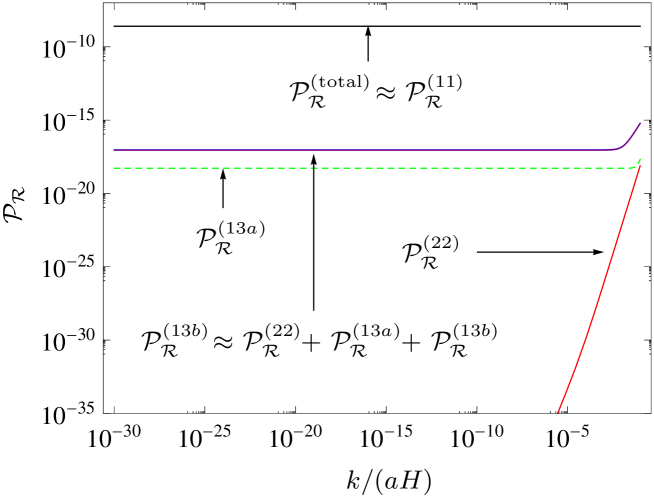
Figure 2: Total second order power spectrum and the contributions from non-linear corrections are shown for scales between the horizon scale to $10^{30}$ factor larger than the horizon scale at, say, the end of inflation; this covers the scales relevant to current observations. Note that ${\cal P}_{\cal R}^{(13a)}$ has negative value. We take the absolute value of ${\cal P}_{\cal R}^{(13a)}$ which is denoted by a dashed line. ${\cal P}_{\cal R}^{(22)}$ continues the slope till the large-scale limit. ${\cal P}_{\cal R}^{(22)}+{\cal P}_{\cal R}^{(13a)}+{\cal P}_{\cal R}^{(13b)}$ nearly coincides with ${\cal P}_{\cal R}^{(13b)}$, and ${\cal P}_{\cal R}^{(11)}$ nearly coincides with ${\cal P}_{\cal R}^{({\rm total})}$.

Our result shows that the effect of leading order non-linear terms to the primordial power spectrum due to a single minimally coupled scalar field is completely negligible under our assumptions of the large scale and the slow-roll. Part of the reason can be found in the $[k/(aH)]^{2}$ suppression factor for the nonlinear terms in (2.2) and (2.2). The effect of $[k/(aH)]^{2}$ suppression factor can be either regarded as large scale suppression occurred during the exponential expansion, or rapid decaying in time during the same expansion. That is, during the accelerated expansion a comoving scale rapidly becomes super-horizon scale. Since our leading order non-linear terms already have $[k/(aH)]^{2}$ terms, the non-linear contributions are suppressed during the accelerated stage as the evolution drives the comoving scales to outside the horizon.

We make a brief discussion on the integrands of the non-linear corrections. In the limit $r\to 0$, the leading term of each integrand is $1/r$ and thus is logarithmically divergent. More specifically, if we restrict ourselves to a box of size $L=1/(aH)$, we have terms with $\log\left(kL\right)$ [17]. Thus, if we push the size of the box to literally infinity, we face a divergence coming from infrared region [18]. Indeed, we have checked that as we push the infrared cutoff towards larger and larger scales, the contributions of the non-linear corrections increase. This infrared divergence may be removed with appropriate manipulations, e.g. boundary effects [19].

Conversely, we can find that the integrals in ${\cal P}_{\cal R}^{(13)}$ diverge in the large $r$ limit. This should be regarded as the breakdown of our approximation near and inside the horizon scale. Thus the ultraviolet cutoff we have chosen in (54), horizon scale cutoff, is the maximum value of $r$ we can have: beyond this value, we are probing sub-horizon regime where our approximation is invalid. We may choose more conservative cutoff, for example $10^{-1}aH/k$. The net effect of pushing $r_{\text{max}}$ to a smaller value is to suppress the non-linear corrections, since as mentioned above the integrands in ${\cal P}_{\cal R}^{(13)}$ become bigger at larger $r$.

5 Conclusions

In this note, we have studied the non-linear corrections to the power spectrum of the comoving curvature perturbation produced during single field slow-roll inflation. All the scalar perturbations in the metric and the inflaton field are described in terms of the gauge invariant comoving curvature perturbation ${\cal R}$. If ${\cal R}$ to the linear order is Gaussian, we need up to third order perturbation to describe the leading non-linear contributions to the power spectrum. Under the assumptions of large scale limit and slow-roll approximation, we have solved the equation of ${\cal R}$ perturbatively up to third order. Using these solutions, we have computed the power spectrum ${\cal P}_{\cal R}$ including the leading non-linear corrections. The resulting power spectrum is, on super-horizon scales, dominated by the linear contribution ${\cal P}_{\cal R}^{(11)}$, and the non-linear corrections are negligible. Our study indicates that we can safely rely on linear cosmological perturbation theory to study power spectrum originated from quantum fluctuations.

Acknowledgement

We thank Donghui Jeong, Misao Sasaki, Martin Sloth and Takahiro Tanaka for useful conversations. J.G. is grateful to the Yukawa Institute for Theoretical Physics, Kyungpook National University and Korea Astronomy and Space Science Institute for hospitality where part of this work was carried out. J.G. was supported in part by a VIDI and a VICI Innovative Research Incentive Grant from the Netherlands Organisation for Scientific Research (NWO) and a Korean-CERN fellowship. H.N. was supported by Mid-career Research Program through National Research Foundation funded by the MEST (No. 2010-0000302). J.H. was supported by the Korea Research Foundation Grant funded by the Korean Government (KRF-2008-341-C00022).

References

• [1] A. H. Guth, Phys. Rev.  D 23, 347 (1981) ; A. D. Linde, Phys. Lett.  B 108, 389 (1982) ; A. Albrecht and P. J. Steinhardt, Phys. Rev. Lett.  48, 1220 (1982).
• [2] For a review, see e.g. D. H. Lyth and A. Riotto, Phys. Rept.  314, 1 (1999) [arXiv:hep-ph/9807278].
• [3] A. H. Guth and S. Y. Pi, Phys. Rev. Lett.  49, 1110 (1982) ; S. W. Hawking, Phys. Lett.  B 115, 295 (1982) ; A. A. Starobinsky, Phys. Lett.  B 117 (1982) 175 ; J. M. Bardeen, P. J. Steinhardt and M. S. Turner, Phys. Rev.  D 28, 679 (1983) ; M. Sasaki, Prog. Theor. Phys.  76, 1036 (1986).
• [4] See e.g. V. F. Mukhanov, H. A. Feldman and R. H. Brandenberger, Phys. Rept.  215, 203 (1992).
• [5] B. Losic and W. G. Unruh, Phys. Rev.  D 72, 123510 (2005) [arXiv:gr-qc/0510078] ; F. Finelli, G. Marozzi, G. P. Vacca and G. Venturi, Phys. Rev.  D 74, 083522 (2006) [arXiv:gr-qc/0604081] ; B. Losic and W. G. Unruh, Phys. Rev. Lett.  101, 111101 (2008) [arXiv:0804.4296 [gr-qc]].
• [6] G. F. Smoot et al., Astrophys. J.  396, L1 (1992) ; E. Komatsu et al., arXiv:1001.4538 [astro-ph.CO].
• [7] C. T. Byrnes, K. Koyama, M. Sasaki and D. Wands, JCAP 0711, 027 (2007) [arXiv:0705.4096 [hep-th]] ; D. Seery, JCAP 0802, 006 (2008) [arXiv:0707.3378 [astro-ph]] ; N. Bartolo, E. Dimastrogiovanni and A. Vallinotto, JCAP 1011, 003 (2010) [arXiv:1006.0196 [astro-ph.CO]].
• [8] R. L. Arnowitt, S. Deser and C. W. Misner, arXiv:gr-qc/0405109.
• [9] J.M. Bardeen, Particle Physics and Cosmology, edited by L. Fang, and A. Zee, (Gordon and Breach, London, 1988), p1.
• [10] H. Noh and J. Hwang, Phys. Rev.  D 69, 104011 (2004) [arXiv:astro-ph/0305123].
• [11] D. Jeong, J. O. Gong, H. Noh and J. c. Hwang, Astrophys. J.  727, 22 (2011) [arXiv:1010.3489 [astro-ph.CO]].
• [12] V. F. Mukhanov, Sov. Phys. JETP 67 (1988) 1297 [Zh. Eksp. Teor. Fiz.  94N7 (1988) 1] ; E. D. Stewart and D. H. Lyth, Phys. Lett.  B 302, 171 (1993) [arXiv:gr-qc/9302019].
• [13] N. D. Birrell and P. C. W. Davies, Quantum Fields in Curved Space (Cambridge University Press, Cambridge, England, 1982).
• [14] J. M. Maldacena, JHEP 0305, 013 (2003) [arXiv:astro-ph/0210603].
• [15] S. B. Giddings and M. S. Sloth, JCAP 1101, 023 (2011) [arXiv:1005.1056 [hep-th]] ; C. T. Byrnes, M. Gerstenlauer, A. Hebecker, S. Nurmi and G. Tasinato, JCAP 1008, 006 (2010) [arXiv:1005.3307 [hep-th]].
• [16] M. S. Sloth, Nucl. Phys.  B 748, 149 (2006) [arXiv:astro-ph/0604488].
• [17] D. H. Lyth, Phys. Rev.  D 45, 3394 (1992) ; L. Boubekeur and D. H. Lyth, Phys. Rev.  D 73, 021301 (2006) [arXiv:astro-ph/0504046] ; D. H. Lyth, JCAP 0712, 016 (2007) [arXiv:0707.0361 [astro-ph]].
• [18] For a review, see e.g. D. Seery, Class. Quant. Grav.  27, 124005 (2010) [arXiv:1005.1649 [astro-ph.CO]].
• [19] Y. Urakawa and T. Tanaka, Prog. Theor. Phys.  122, 779 (2009) [arXiv:0902.3209 [hep-th]] ; Y. Urakawa and T. Tanaka, Phys. Rev.  D 82, 121301 (2010) [arXiv:1007.0468 [hep-th]].
• [20] Y. Tanaka and M. Sasaki, Prog. Theor. Phys.  117, 633 (2007) [arXiv:gr-qc/0612191] ; Y. Tanaka and M. Sasaki, Prog. Theor. Phys.  118, 455 (2007) [arXiv:0706.0678 [gr-qc]] ; Y. i. Takamizu and S. Mukohyama, JCAP 0901, 013 (2009) [arXiv:0810.0746 [gr-qc]] ; Y. i. Takamizu, S. Mukohyama, M. Sasaki and Y. Tanaka, JCAP 1006, 019 (2010) [arXiv:1004.1870 [astro-ph.CO]].