Constraining the S factor of ¹⁵N(p,$\gamma$)¹⁶O at Astrophysical Energies

Abstract

The ¹⁵N(p,$\gamma$)¹⁶O reaction represents a break out reaction linking the first and second cycle of the CNO cycles redistributing the carbon and nitrogen abundances into the oxygen range. The reaction is dominated by two broad resonances at $E_{p}$ = 338 keV and 1028 keV and a Direct Capture contribution to the ground state of ¹⁶O. Interference effects between these contributions in both the low energy region (E_p $<$ 338 keV) and in between the two resonances (338 $<$ E_p $<$ 1028 keV) can dramatically effect the extrapolation to energies of astrophysical interest. To facilitate a reliable extrapolation the ¹⁵N(p,$\gamma$)¹⁶O reaction has been remeasured covering the energy range from E_p=1800 keV down to 130 keV. The results have been analyzed in the framework of a multi-level R-matrix theory and a S(0) value of 39.6 keV b has been found.

I Introduction

The energy production and nucleosynthesis in stars is characterized by nuclear reaction sequences which determine the subsequent phases of stellar evolution. Energy production during the first hydrogen burning phase takes place through the fusion of four protons into helium. This occurs either through the pp-chains or the CNO cycles. The pp-chains dominate hydrogen burning in first generation stars with primordial abundance distributions and in low mass, M$\leq$1.5 M_⊙, stars. The CNO cycles dominate the energy production in more massive, M$\geq$1.5 M_⊙, second or later generation stars with an appreciable abundance of CNO isotopes. The CNO cycles are characterized by sequences of radiative capture reactions and $\beta$-decay processes as shown in Figure Rolfs and Rodney (1988).

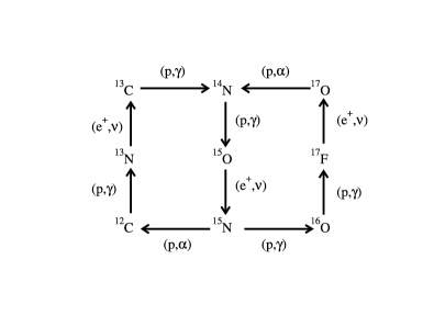
Figure 1: Diagram of the CNO bi cycle Rolfs and Rodney (1988)

At stellar temperatures the ¹⁴N(p,$\gamma$)¹⁵O reaction is the slowest process in the cycle, defining the time scale and the overall energy production rate Imbriani et al. (2004, 2005); Runkle et al. (2005). This reaction is therefore of importance for the interpretation of CNO burning. The proton capture by ¹⁵N is relevant since it is a branch point linking the first CNO or CN cycle with the second CNO, or NO cycle as shown in Figure Rolfs and Rodney (1988) Caughlan and Fowler (1962). This branching has always been a matter of debate since both reactions are characterized by strong low energy resonances.

The reaction rate of ¹⁵N(p,$\alpha$)¹²C is determined by two broad low energy s-wave resonances at E_p = 338 keV and 1028 keV, populating the J^π = 1^- states at 12.44 and 13.09 MeV, respectively, in the ¹⁶O compound nucleus. There have been a number of low energy measurements Schardt et al. (1952),  Zyskind and Parker (1979), and Redder et al. (1982) which provide the basis of the present rate in the literature Caughlan and Fowler (1988); Angulo et al. (1999). Recently, three lower energy points were derived from an indirect “Trojan Horse Method (THM)” Cognata et al. (2009) which are consistent with low energy data Schardt et al. (1952); Zyskind and Parker (1979); Redder et al. (1982).

The competing ¹⁵N(p,$\gamma$)¹⁶O reaction decays predominately to the ground state of ¹⁶O and exhibits the same two resonances but in addition is expected to have a strong non-resonant direct capture component Rolfs and Rodney (1974). The presently available low energy cross section data from Hebbard (1960), Brochard et al. (1973), and Rolfs and Rodney (1974) differ substantially at lower energies. This poses difficulties for a reliable extrapolation of the cross section towards the stellar energy range. An extrapolation was performed Rolfs and Rodney (1974) using a two level Breit-Wigner formalism taking into account the direct capture contribution. The present reaction rate for ¹⁵N(p,$\gamma$)¹⁶O  Angulo et al. (1999) relies entirely on the predictions of Rolfs and Rodney (1974).

To reduce the uncertainty in the strength of the direct capture term single-particle transfer reactions have been performed  Mukhamedzhanov et al. (2008) to determine the proton Asymptotic Normalization Coefficient (ANC) for the ground state of ¹⁶O. With this ANC value $C_{p_{1/2}}^{2}=(192\pm 26)$ fm^-1, R-matrix fits to the ¹⁵N(p,$\gamma$)¹⁶O data have been performed Mukhamedzhanov et al. (2008) which resulted in smaller values for the low energy cross section than those obtained by Rolfs and Rodney (1974). This result was confirmed by an independent R-matrix analysis of the existing data Barker (2008). This conclusion was furthermore supported by a study in which both the (p,$\alpha$) and (p,$\gamma$) reactions were analyzed simultaneously with a multi-level, multi-channel R-matrix formalism Simpson (2006).

Low energy data points were extracted from a re-analysis Bemmerer et al. (2009) of a study of ¹⁴N(p,$\gamma$)¹⁵O performed at the LUNA underground accelerator facility at the Gran Sasso laboratory. This experiment was performed using a windowless differentially pumped gas target with natural nitrogen gas. For detecting the $\gamma$-ray signal, a large BGO scintillator detector was used to observe the characteristic $\gamma$ decay in summing mode Keinonen and Anttila (1976). Since the natural abundance of ¹⁵N is low, the yield of the ¹⁵N(p,$\gamma$) signal was weak and overshadowed by beam induced background yield from proton capture reactions on target impurities and from the ¹⁴N(p,$\gamma$) reaction. The measurements were therefore limited to energies below 230 keV. The proposed cross section results are clearly lower than the values obtained by Rolfs and Rodney (1974) but also slightly lower than the results of Hebbard (1960) and Brochard et al. (1973). Given the strong background conditions, the results could not be normalized to the known on-resonance yield at 338 keV and systematic errors in the data cannot be excluded.

Because of the inconsistencies in the existing data and the uncertainties of an R-matrix analysis based on these existing data, we have performed a new study of the ¹⁵N(p,$\gamma$)¹⁶O over a wide energy range using high resolution Ge detectors. In the following section the experimental approach at the Notre Dame Nuclear Science Laboratory (NSL) and the LUNA II facility at the Gran Sasso underground laboratory will be discussed. This will be followed by a discussion of the experimental data. In the last section the stellar nuclear reaction rate based on the present data will be calculated and compared with existing results.

II Experimental Setup

II.1 Accelerators and Experimental Setup

The experiment was performed at two separate facilities. At the University of Notre Dame the 4 MV KN Van de Graaff accelerator provided proton beams in an energy range of 700 to 1800 keV with beam intensities limited to $\leq$10 $\mu$A on target because of the high count rate in the Ge detector from the ¹⁵N(p,$\alpha_{1}\gamma$)¹²C reaction. The energy calibration of this machine was established to better than 1 keV using the well known ²⁷Al(p,$\gamma$)²⁸Si resonance at 992 keV Keinonen and Anttila (1976). The 1 MV JN Van de Graaff accelerator at Notre Dame was used in the range of 285 keV to 700 keV with protons beams of 20 $\mu$A. The energy of the this machine was calibrated using the well known ¹⁵N(p,$\alpha_{1}\gamma$)¹²C resonance at 429 keV Ajzenberg-Selove (1986).

The LUNA II facility Costantini et al. (2009), located in the Gran Sasso National Laboratory, uses a high current 400 kV, Cockroft- Walton type accelerator. The accelerator provided proton beam currents on target of up to 200 $\mu$A in the energy range of 130 to 400 keV. In addition to the high beam output, the accelerator is extremely stable, and the voltage is known with an accuracy of about 300 eV.

The experimental setup in both experiments was very similar. The targets were water cooled and mounted at 45^∘ with respect to the beam direction. At Notre Dame the position of the beam on the target was defined by a set of vertical and horizontal slits. The beam was swept horizontally and vertically across a target area of 1 cm² by steerers in order to dissipate power over a large target area. At LUNA the ion beam optics provided a de-focused beam on target and no beam sweeping was applied. To avoid the build-up of impurities on the target a Cu finger, cooled to LN₂ temperatures, was placed along the inside of the beamline extending as close to the target as possible. In addition, a bias voltage of about -400 V was applied to the isolated cold finger to suppress the secondary electrons ejected from the target due to proton bombardment.

II.2 Targets

The Ti¹⁵N targets were fabricated at the Forschungszentrum Karlsruhe by reactive sputtering of Ti in a Nitrogen atmosphere enriched in ¹⁵N to 99.95%. The stoichiometry was analyzed using Auger electron spectroscopy to confirm the composition. This test was performed on two target spots, one which had been exposed to beam and one which was not exposed. The results agreed within $\leq$2$\%$ with the nominal stoichiometry of 1:1. Isotopic abundances were experimentally verified by comparing the yield of the ¹⁴N(p,$\gamma)^{15}$O, 278 keV resonance Imbriani et al. (2005) from the enriched targets with that obtained using a target produced with a natural nitrogen gas. The results of this measurement showed an abundance of $\leq$ 2% of ¹⁴N for the thin targets corresponding to a ¹⁵N enrichment of $\geq$ 98% in agreement with the quote of the supplier. For the thick target used at LUNA, ¹⁴N and ¹⁵N enrichment of 17.4 $\pm$ 2.0% and 82.6 $\pm$ 2.0% were found, respectively, most likely caused by a contamination of the enriched gas during sputtering.

 

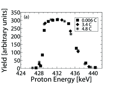
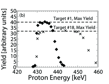
Figure 2: Notre Dame target (left) has a measured width of approximately 7.2 keV at E_p = 430 keV. Squares, diamonds, and stars correspond to 0.006 C, 3.4 C, and 4.8 C of accumulated charge on the target, respectively. LUNA thin (right, diamonds) and thick (right, crosses) targets have measured widths of approximately 9.5 keV, and approximately 25 keV, respectively. The difference in stoichiometry between the two targets can be seen by comparing the plateau heights from the same resonance scan of each target (right).

The thicknesses of all TiN targets were measured using the narrow ¹⁵N(p,$\alpha_{1}\gamma$)¹²C resonance at 429 keV Ajzenberg-Selove (1986). The target used at Notre Dame had a thickness of 7.2 $\pm$ 0.3 keV at E_p = 429 keV and the two targets used at LUNA had thicknesses of 9.5 $\pm$ 0.4 keV and 24.8 $\pm$ 0.5 keV at 429 keV, respectively. The stability of the Notre Dame targets was checked continuously during the course of the experiment using the ¹⁵N(p,$\alpha_{1}\gamma$)¹²C resonance. The thin LUNA target was monitored by rescanning the top of the 338 keV resonance in ¹⁵N(p,$\gamma$)¹⁶O. The thick LUNA target could also be monitored using the ¹⁴N(p,$\gamma$)¹⁵O resonance at E_p = 278 keV because of the large ¹⁴N content (17%) of this target. Because of the relatively low power density delivered at Notre Dame, the target saw virtually no degradation over the experiment with an accumulated charge of 5 C (see Figure 2) and no yield corrections were necessary. During the LUNA experiment with significantly higher beam currents, the thickness of the thin target was reduced by 27$\%$ after an accumulated charge of 17 C and that of the thick target by 30$\%$ after an accumulated charge of 65 C (see Figure 3).

Figure 3: Targets scans of thick target (18) using the ¹⁴N(p,$\gamma)^{15}$O, E_p = 278 keV resonance. The target was stable until about 20 C, and went through significant deterioration. Squares represent the initial target scan, while down triangles represent the scan after 65 C on target

II.3 Detectors

At the NSL, the $\gamma$-rays were observed using a HPGe Clover detector, which consists of four HPGe crystals contained in the same cryostat. This unique arrangement allows the separate detectors to be used in so called add-back mode Dababneh et al. (2004). At LUNA, a single crystal, 115% HPGe detector from Bochum, Germany was used for the detection of $\gamma$-rays. Several sample spectra are given in Figure 4.

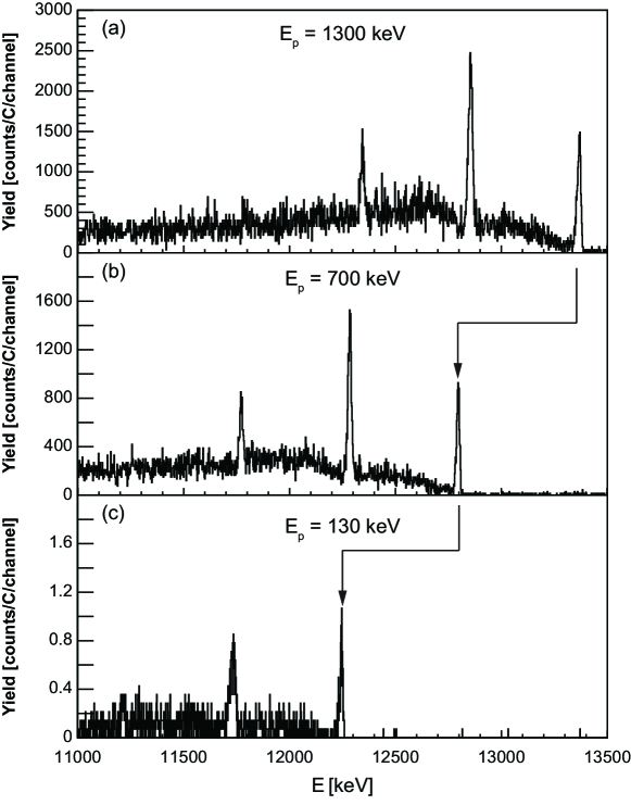
Figure 4: Several sample spectra from the present ¹⁵N(p,$\gamma$)¹⁶O experiment. The spectra were taken with Notre Dame’s KN accelerator (E_p = 1300 keV, top), Notre Dame’s JN accelerator (E_p = 700 keV, middle), and the LUNA II accelerator (E_p = 130 keV, bottom). The ¹⁵N(p,$\gamma$)¹⁶O ground state transition $\gamma$-ray peak is indicated in each spectrum with an arrow.

The primary advantage of the LUNA II facility is the low background environment created by the rock cover from the Gran Sasso mountains. The rock shields from cosmic rays and therefore decreases the $\gamma$-induced background from cosmic rays in the detector and has been shown Bemmerer et al. (2005) to suppress the E_γ > 3.5 MeV background count rate in a Ge detector by three orders of magnitude. In each experiment the detectors were set up at an angle of 45^∘ with respect to the beam direction, allowing the position of the detector to be set as close as possible to the reaction position. The relative efficiency of the $\gamma$-ray detector systems was measured using radioactive sources along with well known capture $\gamma$ reactions. At Notre Dame the relative efficiencies for high energy $\gamma$-rays were established using the ²⁷Al(p,$\gamma$)²⁸Si resonances at 992 keV Keinonen and Anttila (1976) and 1183 keV Meyer et al. (1975) and the ²³Na(p,$\gamma$)²⁴Mg resonance at 1318 keV Zijderhand et al. (1990). The efficiency was extended to a $\gamma$-energy of 12.79 MeV using the ¹¹B(p,$\gamma$)¹²C reaction at 675 keV and 1388 keV following the method of reference  Zijderhand et al. (1990). At LUNA the higher energy efficiencies were determined using the 278 keV resonance in ¹⁴N(p,$\gamma$)¹⁵O  Imbriani et al. (2005)] and the 163 keV resonance in ¹¹B(p,$\gamma$)¹²C  Ajzenberg-Selove (1986). The ¹¹B resonance has a small angular distribution Cecil et al. (1985), and the correction for the relative intensity is less than 3%.

While summing is not of concern for the ground state transition of the ¹⁵N(p,$\gamma$)¹⁶O reaction itself, summing plays a significant role in the determination of the $\gamma$-efficiency. For this reason the efficiency measurements at both laboratories were carried out at several different detector-target distances and the data were simultaneously fitted for all distances following the procedure described by Imbriani et al. Imbriani et al. (2005) (see Figure 5). For the 1 cm and 5 cm measurements, there is one point which has significant summing corrections. This point corresponds to the ground state transition in the E_p = 278 keV ¹⁴N(p,$\gamma$)¹⁵O reaction. While the ground state transition of this reaction has a small branching ratio, each of the other cascades have significant probabilities, which lead to strong summing effects Imbriani et al. (2005).

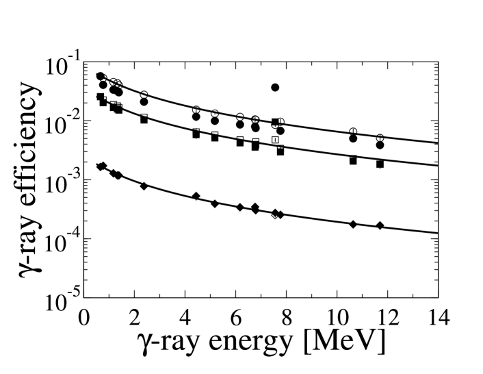
Figure 5: Efficiency curves obtained at LUNA. Circles are measurements at a distance of 1 cm, squares at 3 cm, and diamonds at 20 cm. Closed symbols represent data without summing corrections, open symbols include summing corrections.

III Experimental Results

III.1 Cross Section Determination

The excitation function for the ground state transition of the reaction ¹⁵N(p,$\gamma$)¹⁶O has been measured in the energy range of 131 to 1800 keV. It consists of three distinct, overlapping sections, LUNA data from 131 keV to 400 keV, JN data from 285 keV to 700 keV, and KN data from 700 to 1800 keV. The experimental yield Y (number of reactions per projectile) at proton energy E_p corresponds to the cross section $\sigma$(E) integrated over the target thickness $\Delta$:

$$Y(E_{p})=\int_{E_{p}-\Delta}^{E_{p}}\frac{\sigma(E)}{\epsilon(E)}dE=\sigma(E_{p})\int_{E_{p}-\Delta}^{E_{p}}\frac{f(E)}{\epsilon(E)}dE,$$ (1)

where $\epsilon$ is the stopping power Ziegler, James  F. (2008), and f(E) represents the energy dependence of the cross section in the integration interval:

$$\sigma(E)=\sigma(E_{p})f(E),$$ (2)

with $\sigma$(E_p) the cross section at E_p. This reduces to the well known thin target yield equation if the cross section is constant over the target thickness, f(E)=1. However, at energies where the cross section varies significantly over the target thickness,the yield has to be corrected to extract the cross section. This correction factor is given by:

$$1/\int_{E_{p}-\Delta}^{E_{p}}\frac{f(E)}{\epsilon(E)}dE$$ (3)

and requires the knowledge of the energy dependence of the cross section in the energy interval $\Delta$, f(E). This problem can be solved by an iterative method. In a first step f(E)=1 is assumed resulting in an approximation of the cross section which in turn can be used to calculate a new correction factor. This process is continued until no change in the resulting cross section is obtained. This process quickly converges after 2 to 3 iterations. The resulting cross section is shown in Figure 6.

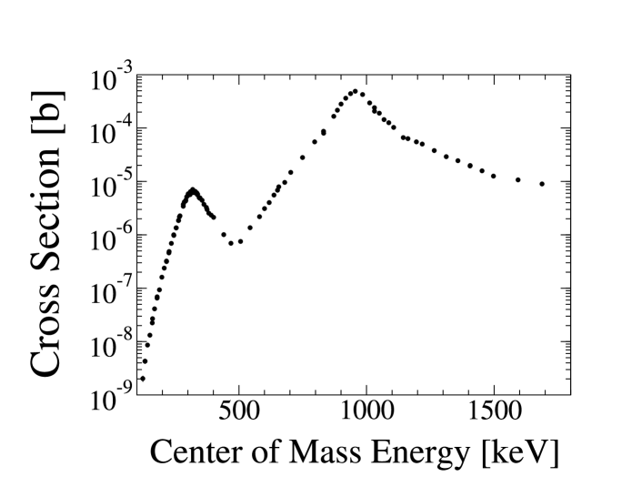
Figure 6: Cross section for the ground state transition of the ¹⁵N(p,$\gamma_{0}$)¹⁶O reaction versus center of mass energy.

An alternative method to determine the cross section was used in which the data were analyzed following the approach described in Imbriani et al. (2005). Here, a brief review of the method is given, which consists of the analysis of the shape of the $\gamma$-line.

The cross section, the stopping power of protons in TiN, the $\gamma$-ray efficiency, and the detector resolution all have an influence on the $\gamma$-ray line shape observed in a spectrum. The observed energy of the $\gamma$-ray is related to the proton energy by Rolfs and Rodney (1988)

$$E_{\gamma}=E_{p}\frac{M}{M+m}+Q-E_{x}-\Delta E_{Rec}+\Delta E_{Dop}$$ (4)

The number of counts N_i in channel i of the $\gamma$-spectrum, corresponding to the energy bin E_γi to E_γi + $\delta$E_γ ($\delta$E = dispersion in units of keV per channel) is given by the expression

$$N_{i}~{}=~{}\frac{\sigma(E_{pi})\delta E_{\gamma}\eta_{fep}(E_{\gamma i})b_{j}}{\epsilon(E_{pi})}$$ (5)

for E${}_{pi}\leq$ E_p (E_pi = proton energy corresponding to channel i, E_p = incident proton energy), where $\sigma(E_{pi})$ is the capture cross section, $\eta_{fep}(E_{\gamma i})$ is the $\gamma$-ray detection efficiency, $\epsilon(E_{pi})$ is the stopping power and b_j is the branching of the associated decay. The conversion from E_γi to E_pi includes the Doppler and recoil effects. The result is folded with the known detector resolution $\Delta$E_γ to obtain the experimental line-shape.

Finally, to infer the cross section in the energy window defined by the target thickness, the cross section was written as the sum of two resonance terms and a constant, non-resonant term as described in Rolfs (1973). In these fits, the free parameters were the non-resonant astrophysical S factor and the gamma-ray background parameters. The results of both methods are in excellent agreement.

The absolute cross section for the ¹⁵N(p,$\gamma$)¹⁶O reaction has been measured on top of the two broad resonances at proton energies of 338 keV and 1028 keV using two independent well known reaction standards and two independent methods. All measurements were performed at three distances (d = 1 cm, 5 cm, 20 cm) to check for systematic errors. The exception to this protocol was the ¹⁵N(p,$\gamma$)¹⁶O measurement at E_p = 338 keV, where the yield at 20 cm was too low. In the first method the cross sections were determined relative to the thick target yield Y_∞(²⁷Al) of the well known ²⁷Al(p,$\gamma$)²⁸Si resonance at 992 keV:

$$Y_{\infty}(^{27}Al)=\frac{\lambda^{2}(E_{R})}{2\epsilon(E_{R})}\frac{M+m}{M}\omega\gamma_{R},$$ (6)

with m (M) the mass of the projectile (target), $\lambda$ the DeBroglie resonance wave length and $\omega\gamma_{R}$ the resonance strength. Adopting the resonance strength of 1.93 $\pm$ 0.13 eV from Paine and Sargood (1979); Antilla et al. (1977); Keinonen and Anttila (1976) the cross sections values of $\sigma_{338}$=6.7 $\pm$ 0.6 $\mu$b and $\sigma_{1028}$=446 $\pm$ 40 $\mu$b are obtained. The errors include the statistical error ($\leq$ 3 $\%$), the error on the relative efficiency (2 $\%$), the error on the relative charge measurement (2$\%$), the uncertainty on stopping power values (5$\%$), and the uncertainty of 7 $\%$ arising from the reference resonance strength of ²⁷Al.

In the second method the cross sections were determined relative to the well known 429 keV resonance in ¹⁵N(p,$\alpha_{1}\gamma$)¹²C Ajzenberg-Selove (1986). In this case the cross section was calculated relative to the integral over the yield curve of the reference resonance, A^ref. The resonance strength $\omega\gamma$ is related to A^ref by:

$$\omega\gamma=\frac{2}{\lambda^{2}}\frac{1}{n_{t}}A^{ref},$$ (7)

with n_t the number of target atoms per cm² which can be calculated from the measured target thickness and the stopping power values. Using this relationship for A^ref (Equation 7), along with Equation 6 and the thin target yield approximation for the ¹⁵N(p,$\gamma$)¹⁶O reaction, the following formula can be derived:

$$\sigma_{(p,\gamma)}(E_{p}) = \left(\frac{\lambda^{2}(E_{R})}{2}\right)\left(\frac{M+m}{M}\right)$$

$$\times\left(\frac{\eta(4.4MeV)}{\eta(12MeV)}\right)\left(\frac{Y(E_{p})}{A^{ref}}\right)\omega\gamma_{R},$$

with $\eta$ the relative $\gamma$-ray efficiency. In this approach the result is independent of all target uncertainties. The yield of the 4.4 MeV $\gamma$-rays from the ¹⁵N(p,$\alpha_{1}\gamma$)¹²C was corrected for the well known angular distribution  Barnes et al. (1952); Kraus et al. (1953). Using the resonance strength of $\omega\gamma_{R}$=21.2 $\pm$ 1.4 eV from Becker et al. (1995), values of $\sigma_{338}$=6.4 $\pm$ 0.6 $\mu$b and $\sigma_{1028}$=436 $\pm$ 44 $\mu$b are obtained. The errors include the statistical error ($\leq$ 3 $\%$), the error of the relative efficiency (2 $\%$), the error of the relative charge measurement (2$\%$), the error of A_ref owing to the numerical integration and angular distribution correction (6$\%$) and the uncertainty of 7 $\%$ of the reference value Becker et al. (1995).

The weighted average of the results from the two methods gives final values of $\sigma_{338}$ = (6.5 $\pm$ 0.3) $\mu$b (5%) and $\sigma_{1028}$ = (438 $\pm$ 16) $\mu$b (4%) taking into account common error sources. The present results are compared to previous values Hebbard (1960); Rolfs and Rodney (1974); Brochard et al. (1973) in Table 1 and are in very good agreement. An exception is the cross section at 338 keV from Rolfs and Rodney Rolfs and Rodney (1974) which is about 50% higher than the other values. This discrepancy will be discussed in more detail in the next section. Data from LUNA and the Notre Dame JN accelerators were normalized to the low energy resonance, while data from the Notre Dame KN accelerator were normalized to the higher energy resonance. Good agreement between the data sets was found at the overlapping energies around 700 keV.

ER	Present	Rolfs	Brochard	Hebbard
		Rolfs and Rodney (1974)	Brochard et al. (1973)	Hebbard (1960)
unit:[keV]	[$\mu$b]	[$\mu$b]	[$\mu$b]	[$\mu$b]
338	6.5 $\pm$ 0.3	9.6 $\pm$ 1.3	6.3*	6.5 $\pm$ .3†
1028	438 $\pm$ 16	420 $\pm$ 60	490*	-

Table 1: Summary of present resonance cross sections in comparison to previous results. *No uncertainty is given. ^† error derived from given reproducibility of 5%.

III.2 Branching Ratios

In previous experiments small cascade transitions have been observed for the broad resonances at 338 keV and 1028 keV Ajzenberg-Selove (1986). For the 338 keV resonance a branching ratio of (1.2 $\pm$ 0.1) $\%$ for the transition to the 6050 keV level was found, in good agreement with the literature value of 1.2 $\pm$ 0.4 $\%$ Ajzenberg-Selove (1986). For the 1028 keV resonance, branches to the 6050 keV level (1.0 $\pm$ 0.3) $\%$ and to the 7118 keV level (2.8 $\pm$ 0.3) $\%$ were measured, and were also in good agreement with literature value of (1.4 $\pm$ 0.4) $\%$ and (3.1 $\pm$ 0.8) $\%$, respectively Ajzenberg-Selove (1986).

III.3 Angular Distributions

In previous analyses of the ¹⁵N(p,$\gamma_{0}$)¹⁶O reaction Rolfs and Rodney (1974); Barker (2008); Mukhamedzhanov et al. (2008), a direct capture component was required to fit the data. In each of these cases, only the l_i = 0 initial wave was included in the calculation. This component represents s-wave capture, and therefore interferes with the resonant component of the cross section. The s-wave components yield isotropic $\gamma$-ray distributions Rolfs (1973); Rolfs and Rodney (1974). However, an $l_{i}$ = 2 direct capture component is allowed for E1 transitions, and can contribute to the reaction, possibly introducing some anisotropy in the gamma decay. In looking for this signature, the set-up was tested using the 1 MeV resonance, which is reported to be isotropic Rolfs and Rodney (1974). Measurements were made with the central Clover axis at several angles relative to the beam direction with a nominal distance of 5 cm. To extract additional data points, the add-back feature was used to treat the left and right halves of the Clover system as separate detectors, where Monte Carlo calculations using the code GEANT4 Geant4 Collaboration et al. (2003) yielded an effective angular offset of each half from the central detector axis of 15^∘. Measurements with a calibrated ¹³⁷Cs source, and the isotropic 278 keV resonance of ¹⁴N(p,$\gamma$)¹⁵O made corrections to the absorption effects possible. The results confirmed the isotropy of the angular distribution of the ground state decay $\gamma$-rays from the 1028 keV resonance in ¹⁵N(p,$\gamma_{0}$)¹⁶O.

In the search for the l_f = 2 component, angular distribution measurements of ¹⁵N(p,$\gamma_{0}$)¹⁶O were made at a proton energy of 540 keV at detection angles of 0^∘, 45^∘, and 90^∘ relative to the beam axis. With two Clover segments, this resulted in 6 data points. Two of these points were excluded due to large absorption effects from the shape of the target chamber. The resulting angular distribution was fit with a function of the form W($\theta$) = a${}_{0}^{exp}$ + a${}_{2}^{exp}$ P₂(cos$\theta$), where P₂ is the L = 2 Legendre polynomial, and a${}_{2}^{exp}$= Q₂ a₂, where Q₂ is the usual geometrical correction factor due to the finite size of the detector Ferguson (1965). The Q₂ term can be directly determined using the ¹⁶O(p,$\gamma$) DC $\rightarrow$ 495 keV reaction Rolfs (1973). This reaction has a well known angular distribution of the form $W(\theta)=sin^{2}(\theta)$. Plotting the measured W$(\theta)$ with respect to $sin^{2}(\theta)$, the deviation of the slope from 1.0 gives directly the $Q_{2}$ value. Using the left and right Clover halves to measure the ¹⁶O(p,$\gamma$)¹⁷F DC$\rightarrow$495 keV a value of Q₂ = 0.975$\pm$0.020 was found. This results in an a₂ value for the ¹⁵N(p,$\gamma_{0}$)¹⁶O reaction at 540 keV of 0.08 $\pm$ 0.10, which is consistent with isotropy.

IV R-Matrix Analysis

An R-matrix analysis was performed which mirrored the procedure of previous analyses Rolfs and Rodney (1974); Barker (2008); Mukhamedzhanov et al. (2008). This analysis included the two broad 1^- resonance levels and a direct capture contribution. The analysis was performed with the multi-channel R-matrix code AZURE Azuma et al. (2010). Details of the theory and the nomenclature are given in Azuma et al. (2010) and references therein. The best fit results can be seen in Figure 7 where the cross sections have been converted to the astrophysical S-factor. This fit results in an S(0) value of 39.6 keV b.

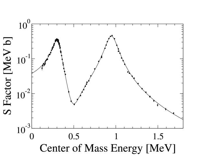
Figure 7: Experimental S factor for the ground state transition of the ¹⁵N(p,$\gamma_{0}$)¹⁶O reaction shown together with the best fit results of an R-matrix calculation using the code AZURE.

Looking closer at the low energy region (see Figure 8) and comparing the results to previous experiments, the low energy data of Rolfs and Rodney (1974) are inconsistent with the present results. While this data set agrees very well at higher energies it starts to deviate below a proton energy of 400 keV. There is no obvious reason for this inconsistency but it should be noted that the low energy data of Rolfs and Rodney Rolfs and Rodney (1974) carry a significant uncertainty in this region. The data of Hebbard Hebbard (1960) are in reasonably good agreement above 230 keV. The data of Brochard Brochard et al. (1973) show good agreement except for the three data points below the 338 keV resonance which show a large scatter.The recent Bemmerer data Bemmerer et al. (2009) are systematically lower than the present data, and also seem to have a slightly different energy dependence.

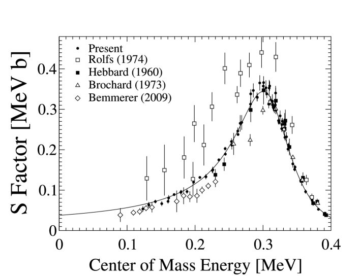
Figure 8: Low energy region of present data set (filled circles) shown with AZURE R-matrix calculation along with previous measurements of Rolfs Rolfs and Rodney (1974)(open squares), Hebbard Hebbard (1960)(filled squares), Brochard Brochard et al. (1973)(open triangles), and Bemmerer Bemmerer et al. (2009)(open diamonds) in the region of 0 - 400 keV

The parameters for the best fit are given in Table 2. With the exception of the first resonance, most parameters are in fair agreement with previous results Mukhamedzhanov et al. (2008); Barker (2008). The width of the first resonance is dominated by the alpha width Ajzenberg-Selove (1986). This parameter is, therefore, well constrained by the present (p,$\gamma$) data. The resonance strength, however, is determined by the product of the proton and $\gamma$ width. Without including proton scattering data in the fit, these parameters are not well constrained. However, it should be noted that tests showed that this ambiguity has no influence on the extrapolation of the data. In these tests, the proton width ($\gamma_{p_{1}}$) was fixed at different values while allowing the other parameters to vary. For the higher energy resonance the proton and alpha width are comparable, which provides more of a constraint on the parameters. In addition, the present result for the ground state ANC is significantly larger than the value of Mukhamedzhanov et al. (2008) which cannot be attributed to the choice of radius (see below). While these differences do not have an impact on the extrapolation of the S-factor to lower energies, a more thorough analysis is warranted for the interpretation of the R-matrix parameters. This will be addressed in a forthcoming publication LeBlanc where the results of simultaneous multi-channel fits to all relevant reaction channels will be presented.

Reference	E1	$\gamma^{2}_{p_{1}}$	$\gamma^{2}_{{\alpha_{0}}_{1}}$	$\gamma^{2}_{\gamma_{1}}$(int)	$\Gamma_{\gamma_{1}}$	E2	$\gamma^{2}_{p_{2}}$	$\gamma^{2}_{{\alpha_{0}}_{2}}$	$\gamma^{2}_{\gamma_{2}}$(int)	$\Gamma_{\gamma_{2}}$	Cg.s[fm1/2]	$\theta_{g.s}$
	Jπ = l-	lp = 0	lα = 1			Jπ = l-	lp = 0	lα = 1			s,d$\rightarrow$p
Present	12.438	52.8	13.5	51.3	33.8	13.087	309.1	5.0	34.1	38.7	23.22	0.608
Mukhamedzhanov et al. (2008)	12.439	280.9	12.5	-	8.8$\pm$1.5	13.089	271.4	6.1	-	50$\pm$8	13.85	-
(Barker, 2008, RR)	12.452	93.6	13.5	38.0	-	13.111	416.0	0.812	0.5	-	-	1.944
(Barker, 2008, HH)	12.447	355.2	10.6	7.2	-	13.087	265.2	5.4	56.2	-	-	0.569

Table 2: Best fit R-matrix parameters for the ¹⁵N(p,$\gamma$)¹⁶O reaction (E_x in MeV, $\gamma^{2}_{i}$ in keV). Channel radii of $a_{p}=5.030$ fm and $a_{\alpha}=6.500$ fm were used in the fit. The boundary condition BC in the fit was chosen to be equal to the shift function at the energy of the lowest J^π=1^- resonance. Because of this choice of BC, the $\Gamma_{\gamma_{1}}$ (in eV) can be calculated directly from the reduced width amplitude while $\Gamma_{\gamma_{2}}$ is calculated from the Barker transformation of the reduced width amplitude Azuma et al. (2010). The parameters shown in this table are mainly intended to enable the reader to reproduce the fit presented in this manuscript, and should not be regarded as final. With respect to the physical interpretation of these fit parameters, a detailed discussion will be presented in a forthcoming paper LeBlanc .

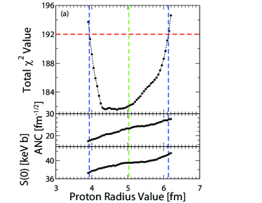
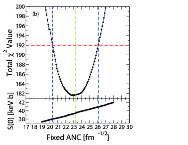
Figure 9: Dependence of AZURE fits on key parameters used in the fits. Parameters were varied noting that for a 9 parameter fit, a 70% confidence region is defined for $\approx$ $\chi^{2}$ = $\chi^{2}_{min}$ + 10 James (1994). Even though a lower $\chi^{2}$ was found with a radius of about 4.4 fm, 5.03 was chosen so as to be more comparable to Barker (2008). ANC was found to be (23 $\pm$ 3) fm^-1/2. Fixing the ANC to the value found in Mukhamedzhanov et al. (2008) gives a $\chi^{2}$ that is much higher than the current best fit value.

In the present parameter space the only non-s-wave contribution arises from the d-wave component of the direct capture. Using the parameters for the best fit the $\gamma$-ray angular distribution was calculated at the minimum of the cross section between the two resonance at 540 keV yielding a value of a₂ = 0.034. The result is consistent with the experimental upper limit of 0.18 (see Section III C).

The sensitivity of the best fit was tested against several key parameters. In multi-parameter fitting, uncertainties of specific parameters are determined in terms of confidence regions. For a nine parameter fit (E_λ,$\gamma_{i}$ for both levels plus ANC or $\theta_{g.s.}$) a 70% confidence region for one of the parameters is defined by the range where $\chi^{2}$ $\leq$ $\chi^{2}_{min}$ + 10 James (1994). The degrees of freedom is 102 (113 data points, 9 parameters) resulting in a reduced $\chi^{2}$ of 1.8.

Radii of r_p = 5.03 fm, and r_α = 6.5 fm, were taken from Barker (2008). The dependence of the fit on the proton radius was tested, and the results are given in Figure 9. Any proton radius value between 4 and 6 fm is considered acceptable. Variation of the radius over this range corresponds to only a 5% uncertainty in the S(0) extrapolation. This test also showed that the ANC is not very sensitive to the choice of the radius. The best fit gives a ground state ANC of (23 $\pm$ 3) fm^-1/2 (corresponding to a reduced width amplitude of $\theta_{g.s.}$ = 0.61). The error associated with the ANC was determined by fixing the ANC at different values, and finding a new best fit. The results of this procedure can be seen in Figure 9. Even though the results give a 13% uncertainty for the ANC, the variation in S(0) from this procedure is only 4%.

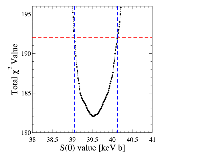
Figure 10: Variation of $\chi^{2}$ with extrapolated S(0) values (for details, see text).

To evaluate the uncertainty of the fit itself, fits were performed which were forced to result in different S(0) values by inserting a fake data point at 1.5 keV with extremely small errors. The small error of this data point forces the calculation to match this fictitious data point and thus vary the extrapolation. By varying the fictitious point and observing the change in the $\chi^{2}_{tot}$, the experimental uncertainty of the extrapolation can be determined (see Figure 10). This results in an uncertainty of $\pm$ 0.6 keV b. Including the 5% error of the absolute cross section gives a final S(0) value of (39.6 $\pm$ 2.6) keV b. This value is compared in Table 3 with previous extrapolations Hebbard (1960); Rolfs and Rodney (1974); Simpson (2006); Barker (2008); Mukhamedzhanov et al. (2008). The present result is in good agreement with the original value of Hebbard Hebbard (1960), the Barker Barker (2008) analysis of the Hebbard data (labelled HH in Table 3, and the results of Mukhamedzhanov et al. Mukhamedzhanov et al. (2008). The extrapolation of the Rolfs and Rodney data Rolfs and Rodney (1974) (Rolfs and Rodney Rolfs and Rodney (1974), Simpson Simpson (2006) and Barker Barker (2008), labelled RR in Table 3) are all significantly higher because of the larger low energy cross sections used for their fit analysis.

Table 3: Summary of Previous Results for extrapolated S(0) values

Analysis	$S(0)_{\gamma}$ (keV b)
Hebbard 1960 Hebbard (1960)	32
Rolfs 1974 Rolfs and Rodney (1974)	64 $\pm$ 6
Barker 2008 (RR) Barker (2008)	$\approx$ 50-55
Barker 2008 (HH) Barker (2008)	$\approx$ 35
Mukhamedzhanov Mukhamedzhanov et al. (2008)	36.0 $\pm$ 6.0
Present	39.6 $\pm$ 2.6

V Reaction Rate

Using the results from the AZURE extrapolations, the reaction rates can be numerically determined using the formalism outlined in Angulo et al. (1999)

$$N_{A}\langle\sigma v\rangle = 3.73\cdot 10^{7}\mu^{-\frac{1}{2}}T^{-\frac{3}{2}}$$

$$\times\int_{0}^{\infty}S(E)e^{(-2\pi\eta)}e^{(-11.605E/T)}dE$$

with $\mu$ the reduced mass, T the temperature in GK, and $\eta$ the Sommerfeld parameter; the results are in cm³ mole^-1 s^-1. The above function was numerically integrated for temperatures between T = 0.01 - 10 GK. The present data covers an energy range of E = 0 to 1.8 MeV, which validates the integration up to a temperature of T = 1 GK. For higher temperatures, the S-factor curve must be extended to higher energies beyond what the present experimental data cover. We followed the procedure of the NACRE compilation Angulo et al. (1999) which handles this difficulty by equating all higher energy S-factor values with the highest energy data point where the cross section varies only slowly with energy. The results are given in Table 4. The present rate is at lower temperatures up to a factor two lower than previous rates reflecting the change in the low energy S-factor.

T9 [GK]	N${}_{A}\langle\sigma v\rangle_{Present}$	N${}_{A}\langle\sigma v\rangle_{NACRE}$	N${}_{A}\langle\sigma v\rangle_{CA88}$
		Angulo et al. (1999)	Caughlan and Fowler (1988)
0.010	2.284E-21	4.33E-21	3.93E-21
0.015	1.377E-17	2.66E-17	2.34E-17
0.020	3.322E-15	6.50E-15	5.61E-15
0.030	3.215E-12	6.41E-12	5.38E-12
0.040	2.456E-10	4.96E-10	4.08E-10
0.050	5.378E-09	1.09E-08	8.90E-09
0.060	5.681E-08	1.16E-07	9.36E-08
0.070	3.747E-07	7.64E-07	6.14E-07
0.080	1.784E-06	3.63E-06	2.91E-06
0.090	6.699E-06	1.36E-05	1.08E-05
0.100	2.104E-05	4.23E-05	3.37E-05
0.150	1.280E-03	2.46E-03	1.92E-03
0.200	1.908E-02	3.52E-02	3.09E-02
0.300	6.143E-01	1.05E+00	1.57E+00
0.400	4.682E+00	7.48E+00	1.45E+01
0.500	1.668E+01	2.58E+01	5.42E+01
0.600	3.908E+01	5.90E+01	1.27E+02
0.700	7.213E+01	1.07E+02	2.25E+02
0.800	1.165E+02	1.68E+02	3.39E+02
0.900	1.763E+02	2.46E+02	4.67E+02
1.000	2.599E+02	3.50E+02	6.18E+02
1.500	1.485E+03	1.67E+03	2.33E+03
2.000	4.735E+03	5.05E+03	6.61E+03
3.000	1.489E+04	1.55E+04	1.97E+04
4.000	2.428E+04	2.27E+04	3.12E+04
5.000	3.064E+04	2.61E+04	3.83E+04
6.000	3.435E+04	2.86E+04	4.19E+04
7.000	3.624E+04	3.06E+04	4.31E+04
8.000	3.699E+04	3.23E+04	4.29E+04
9.000	3.706E+04	3.37E+04	4.19E+04
10.000	3.674E+04	3.51E+04	4.04E+04

Table 4: Table of reaction rates for ¹⁵N(p,$\gamma_{0}$)¹⁶O. Present rates, along with the NACRE Angulo et al. (1999), and CA88 Caughlan and Fowler (1988) results are given.

Following the example of the NACRE compilations, the above results were fit using the following parametrization

$$N_{A}<\sigma v> = a_{1}10^{9}T^{-\frac{3}{2}}exp[a_{2}T^{-\frac{1}{3}}-(T/a_{3})^{2}]$$

$$[1+a_{4}T+a_{5}T^{2}]+a_{6}10^{3}T^{-\frac{3}{2}}$$

$$exp(a_{7}/T)+a_{8}10^{6}T^{-\frac{3}{2}}exp(a_{9}/T),$$

where the best fit parameters can be found in Table 5.

a1 = 0.523	a4 = 6.339	a7 = -2.913
a2 = -15.240	a5 = -2.164	a8 = 3.048
a3 = 0.866	a6 = 0.738	a9 = -9.884

Table 5: Best fit parameters for the ¹⁵N(p,$\gamma_{0}$)¹⁶O reaction rate using the NACRE fitting formulations.

VI Conclusion

The result of this work clearly demonstrates that there are significant uncertainties in the low energy cross section data of radiative capture processes of astrophysical relevance, despite many decades of low energy reaction studies. These uncertainties affect directly our understanding and interpretation of solar and stellar hydrogen burning phenomena. In this case the new results influence primarily the leakage rate from the CN to the ON cycle in stellar burning via the ¹⁵N(p,$\gamma$)¹⁶O radiative capture process, which is reduced by a factor of two compared to the previous rate used traditionally in CNO nucleosynthesis simulations. In particular, the change in rate will modify the equilibrium abundance of ¹⁶O, which is correlated with the leakage rate of ¹⁵N(p,$\gamma$)¹⁶O from the CN cycle and the rate of ¹⁶O(p,$\gamma$)¹⁷F in the NO cycle. However a detailed study of the astrophysical impact of the present measurement goes beyond the aim of the present work, but should benefit from recent studies of low energy reaction rates Azuma et al. (2010).

The reliability of stellar reaction rates depends critically on the quality of the experimental cross section data. Direct measurements of the reaction cross sections at the Gamow range of stellar burning have been successful in only a few cases of reactions between light nuclei. Considering the anticipated count rates for the CNO radiative capture reactions we will continue to rely for most cases on the extrapolation of low energy measurements into the Gamow range. The present analysis clearly demonstrates that this requires a two-fold approach, pursuing the direct reaction measurements to the lowest possible energies in a background shielded environment but also expanding the experimental range of the measurements to determine unambiguously the various reaction components of the radiative capture process. The latter step is essential for minimizing the uncertainties in the R-matrix analysis of the cross section and can be complemented by independent studies which explore independently the strength of specific ”hidden” reaction components such as the direct capture through ANC measurements and analysis.

The approach taken here for the study of the ¹⁵N(p,$\gamma$)¹⁶O reaction has succeeded in combining both the efforts of improving on the extent and quality of the low energy cross section data in underground accelerator experiments. At the same time the study has improved on the detailed measurement of higher energy data providing a better constraint on determining the external capture component and its impact on the low energy extrapolation of the reaction cross section. The combination of these two complementary measurements successfully reduced the overall uncertainty in the ¹⁵N(p,$\gamma$)¹⁶O reaction rate.

We are extremely grateful for the help of the technical staff of both the Nuclear Science Laboratory at the University of Notre Dame and that of the Gran Sasso facility. REA thanks the NSERC for partial financial support through the DRAGON grant at TRIUMF. This work was funded in part by the National Science Foundation through grant number 0758100, the Joint Institute for Nuclear Astrophysics grant number 0822648, along with INFN, Italy.

References

- Rolfs and Rodney (1988) C. E. Rolfs and W. S. Rodney, Cauldrons in the cosmos: Nuclear astrophysics (1988).
- Imbriani et al. (2004) G. Imbriani, H. Costantini, A. Formicola, D. Bemmerer, R. Bonetti, C. Broggini, P. Corvisiero, J. Cruz, Z. Fülöp, G. Gervino, et al., Astronomy and Astrophysics 420, 625 (2004).
- Imbriani et al. (2005) G. Imbriani, H. Costantini, A. Formicola, A. Vomiero, C. Angulo, D. Bemmerer, R. Bonetti, C. Broggini, F. Confortola, P. Corvisiero, et al., European Physical Journal A 25, 455 (2005).
- Runkle et al. (2005) R. C. Runkle, A. E. Champagne, C. Angulo, C. Fox, C. Iliadis, R. Longland, and J. Pollanen, Physical Review Letters 94, 082503 (2005).
- Caughlan and Fowler (1962) G. R. Caughlan and W. A. Fowler, Astrophys. J. 136, 453 (1962).
- Schardt et al. (1952) A. Schardt, W. A. Fowler, and C. C. Lauritsen, Physical Review 86, 527 (1952).
- Zyskind and Parker (1979) J. L. Zyskind and P. D. Parker, Nuclear Physics A320, 404 (1979).
- Redder et al. (1982) A. Redder, H. W. Becker, H. Lorenz-Wirzba, C. Rolfs, P. Schmalbrock, and H. P. Trautvetter, Zeitschrift fur Physik 305, 325 (1982).
- Caughlan and Fowler (1988) G. R. Caughlan and W. A. Fowler, Atomic Data and Nuclear Data Tables 40, 283 (1988).
- Angulo et al. (1999) C. Angulo, M. Arnould, M. Rayet, P. Descouvemont, D. Baye, C. Leclercq-Willain, A. Coc, S. Barhoumi, P. Aguer, C. Rolfs, et al., Nuclear Physics A656, 3 (1999).
- Cognata et al. (2009) M. LaCognata, V. Z. Goldberg, A. M. Mukhamedzhanov, C. Spitaleri, and R. E. Tribble, Phys. Rev. C 80, 012801 (2009).
- Rolfs and Rodney (1974) C. Rolfs and W. S. Rodney, Nuclear Physics A235, 450 (1974).
- Hebbard (1960) D. Hebbard, Nuclear Physics 15, 289 (1960).
- Brochard et al. (1973) F. Brochard, P. Chevallier, D. Disdier, and F. Scheibling, Le Journal de Physique 34, 363 (1973).