Thermodynamic Potential for
     Superfluid ³He in Aerogel

Abstract

We present a free energy functional for superfluid ³He in the presence of homogeneously distributed impurity disorder which extends the Ginzburg-Landau free energy functional to all temperatures. We use the new free energy functional to calculate the thermodynamic potential, entropy, heat capacity and density of states for the B-phase of superfluid ³He in homogeneous, isotropic aerogel.

PACS numbers: 67.30.ef, 67.30.H-, 67.30.hm, 61.43.Hv

Introduction

Liquid ³He infused into high porosity silica aerogel provides us with a model physical system for studying the effects of quenched disorder on an Fermi liquid with unconventional pairing Halperin and Sauls (2004). Indeed ³He-aerogel provides us with a system where the effects of disorder can be explored over the entire range from weak to strong disorder without modifying the basic interactions of the Fermi liquid.

Theoretical analysis by Thuneberg et al. Thuneberg et al. (1998) showed that the effects of scattering by a homogeneous, isotropic medium enhanced the stability of the Balian-Werthamer (BW) phase relative to the anisotropic ABM or Planar phase. These authors also calculated the reduction in the transition temperature, $T_{c}$, the order parameter, $\widehat{\Delta}(\hat{\bf p})$, and condensation energy, $\Delta\Omega(p,T)$, in the Ginzburg-Landau (GL) limit. Experimentally, the equilibrium phase of ³He-aerogel is consistent with the Balian-Werthamer (BW) state, modified by de-pairing, over the entire phase diagram, except perhaps in a narrow region of temperatures near $T_{c}$ at high pressures Sprague et al. (1996); Barker et al. (2000); Sauls et al. (2005). Measurements of the heat capacity of ³He-aerogel at intermediate and high pressures provide quantitative measurements of de-pairing, including the reduction in $\Delta C/\gamma_{\mbox{\tiny N}}T_{c_{0}}$ as well as indirect evidence of gapless excitations with a finite density of states, $N(0)$, at the Fermi energy Choi et al. (2004).

We report results based on a free energy functional which extends the GL theory for superfluid ³He in the presence of homogeneously distributed impurity disorder to all temperatures. This functional is obtained by a reduction of the Luttinger-Ward functional to leading order in the expansion parameters of Fermi-liquid theory. Results for the thermodynamic potential, entropy, heat capacity and density of states for the B-phase of superfluid ³He-aerogel in the weak-coupling limit are reported. For impurity scattering in the unitary limit the B-phase exhibits gapless behavior over the entire phase diagram for high-porosity aerogels with an elastic mean-free path $\ell_{\mbox{\tiny el}}=1500\,\mbox{\AA}$.

Free Energy Functional

Serene and Rainer (SR) obtained a functional of the low-energy, quasiclassical propagator, $\widehat{g}(\hat{\bf p},\epsilon_{n})$, and self-energy, $\widehat{\sigma}(\hat{\bf p},\epsilon_{n})$, for a superfluid Fermi liquid starting from the Luttinger-Ward-DeDominicis-Martin (LWDM) functional Luttinger and Ward (1960); DeDominicus and Martin (1964) of the exact propagator and self energy and subtracting the functional evaluated at the stationarity condition corresponding to the normal Fermi liquid Serene and Rainer (1983). This subtraction confines the functional to the low-energy states near the Fermi surface. Note that $\widehat{\sigma}$, represents corrections to the leading order normal-state self-energy. Similarly, the subtracted $\Phi$-functional can be expressed as a functional of the low-energy propagator and effective interactions represented by block vertices that sum to all orders the bare interaction and higher order processes mediated by the high-energy propagator. So long as the block vertices do not introduce a new low-energy scale, then the contributions to the subtracted $\Phi$-functional can be classified by their order in one or more small parameters of Fermi-liquid theory. The SR functional has the form,

$$\Delta\Omega\bigl{[}\widehat{g},\widehat{\sigma}\bigr{]} = -\frac{\mbox{\footnotesize 1}}{\mbox{\footnotesize 2}}Sp^{\prime}\left\{\widehat{\sigma}\widehat{g}\right\}+\Delta\Omega_{\ln}+\Phi\bigl{[}\widehat{g}\bigr{]}\,,$$ (1)

$$\Delta\Omega_{\ln} = -\frac{\mbox{\footnotesize 1}}{\mbox{\footnotesize 2}}Sp^{\prime}\Bigl{\{}\int d\xi_{{\bf p}}\left[\ln_{\otimes}\left(-i\epsilon_{n}{\widehat{\tau}_{\mbox{\tiny 3}}}+\xi_{{\bf p}}+\widehat{\sigma}\right)-\ln_{\otimes}\left(-i\epsilon_{n}{\widehat{\tau}_{\mbox{\tiny 3}}}+\xi_{{\bf p}}\right)\right]\Bigr{\}}\,,$$ (2)

where $Sp^{\prime}\{...\}\equiv 2N_{f}\int d^{3}R\,\int\frac{d\Omega_{\hat{\bf p}}}{4\pi}\,\pi T\sum_{\epsilon_{n}}\mbox{\sf Tr}_{\mbox{\tiny 4}}\left\{\ldots\right\}$ and $\mbox{\sf Tr}_{\mbox{\tiny 4}}\left\{\ldots\right\}$ is the trace in Nambu space. The SR functional is general enough to describe inhomogeneous equilibrium states of a superfluid Fermi liquid which vary slowly on the atomic scale. In such cases the convolution product attached to the $\ln$-functional is defined as $\widehat{a}\otimes\widehat{b}({\bf p},{\bf R})=\exp\Bigl{\{}\frac{i}{2}\left(\mbox{\boldmath$\nabla$}_{{\bf R}}^{a}\cdot\mbox{\boldmath$\nabla$}_{{\bf p}}^{b}-\mbox{\boldmath$\nabla$}_{{\bf p}}^{a}\cdot\mbox{\boldmath$\nabla$}_{{\bf R}}^{b}\right)\Bigr{\}}$ $\widehat{a}({\bf p},{\bf R})\,\widehat{b}({\bf p},{\bf R})$. For example $\xi_{{\bf p}}\otimes\widehat{a}=(\xi_{{\bf p}}-\frac{i}{2}{\bf v}_{f}\cdot\mbox{\boldmath$\nabla$}_{{\bf R}})\widehat{a}({\bf p},{\bf R})$. The SR functional is stationary with respect to variations of $\widehat{g}$ and $\widehat{\sigma}$. The latter condition generates,

$$\widehat{g}(\hat{\bf p},{\bf R};\epsilon_{n})=\int d\xi_{{\bf p}}\left(i{\widehat{\tau}_{\mbox{\tiny 3}}}\epsilon_{n}-\xi_{{\bf p}}-\widehat{\sigma}\right)_{\otimes}^{-1}\,,$$ (3)

which can be transformed à la Eilenberger into the quasiclassical transport equation Eilenberger (1968), $\Bigl{[}i{\widehat{\tau}_{\mbox{\tiny 3}}}\epsilon_{n}-\widehat{\sigma},\,\widehat{g}\Bigr{]}+i{\bf v}_{f}\cdot\mbox{\boldmath$\nabla$}_{{\bf R}}\widehat{g}=0$, and normalization condition, $\widehat{g}(\hat{\bf p},{\bf R};\epsilon_{n})^{2}=-\pi^{2}\widehat{1}$. Stationarity of the SR functional with respect to variations of the propagator, $\widehat{g}\rightarrow\widehat{g}+\delta\widehat{g}$, identifies the self energy with the skeleton expansion obtained from the $\Phi$-functional,

$$\delta\Phi\bigl{[}\widehat{g}\bigr{]}\equiv\Phi\bigl{[}\widehat{g}+\delta\widehat{g}\bigr{]}-\Phi\bigl{[}\widehat{g}\bigr{]}=\frac{\mbox{\footnotesize 1}}{\mbox{\footnotesize 2}}Sp^{\prime}\{\widehat{\sigma}\delta\widehat{g}\}\,.$$ (4)

To leading order in the small expansion parameter the $\Phi$-functional is given by

$$\Phi_{\mbox{\tiny ff}}=N_{f}\int d^{3}R\,\int\frac{d\Omega_{\hat{\bf p}}}{4\pi}\frac{d\Omega_{\hat{\bf p}^{\prime}}}{4\pi}\,v(\hat{\bf p},\hat{\bf p}^{\prime})\,T\sum_{\epsilon_{n}}^{\prime}{\bf f}(\hat{\bf p},{\bf R};\epsilon_{n})\cdot T\sum_{\epsilon_{n}^{\prime}}^{\prime}\,\bar{{\bf f}}(\hat{\bf p}^{\prime},{\bf R};\epsilon_{n}^{\prime})\,,$$ (5)

where $v(\hat{\bf p}\cdot\hat{\bf p}^{\prime})$ is the odd-parity, spin-triplet pairing interaction, while ${\bf f}(\hat{\bf p},{\bf R};\epsilon_{n})$ and $\bar{{\bf f}}(\hat{\bf p},{\bf R};\epsilon_{n})$ are the spin-triplet components of the the off-diagonal “anomalous” components of the propagator. This functional generates the mean-field pairing self energy,

$$\bm{\Delta}(\hat{\bf p},{\bf R})=\int\frac{d\Omega_{\hat{\bf p}^{\prime}}}{4\pi}v(\hat{\bf p},\hat{\bf p}^{\prime})T\sum_{\epsilon_{n}^{\prime}}^{\prime}\,{\bf f}(\hat{\bf p}^{\prime},{\bf R};\epsilon_{n}^{\prime})\,.$$ (6)

The Matsubara sums include a cutoff, $\Omega_{c}$, that restricts the pairing interaction to the low-energy band near the Fermi level. At this same order the diagonal mean-fields, i.e. the Landau molecular fields, also contribute. These terms are important for states perturbed by external fields or for inhomogeneous phases, but vanish for the homogeneous equilibrium state. For the applications discussed below the Landau molecular field self energy is omitted.

In order to obtain a generalization of the GL functional we invert the self-consistency condition for the anomalous propagator to reduce the SR functional to a functional of the order parameter, $\bm{\Delta}$. Thus, $\Phi_{\mbox{\tiny ff}}$ can be evaluated to give,

$$\Phi_{\mbox{\tiny ff}} = N_{f}\int d^{3}R\,\frac{1}{v_{1}}\int\frac{d\Omega_{\hat{\bf p}}}{4\pi}\,|\bm{\Delta}(\hat{\bf p},{\bf R})|^{2}\,,$$ (7)

for pure p-wave pairing. Similarly, in Eq. (1), $-\frac{\mbox{\footnotesize 1}}{\mbox{\footnotesize 2}}Sp^{\prime}\left\{\widehat{\sigma}\widehat{g}\right\}=-2\Phi_{\mbox{\tiny ff}}$.

In order to include the interaction of liquid ³He with the structure of silica aerogel we explicitly include a one-body interaction, $\widehat{\mbox{\footnotesize{V}}}=\mbox{\footnotesize{V}}\widehat{1}$, representing the interaction of quasiparticles with the static impurity potential, $\mbox{\footnotesize{V}}({\bf p},{\bf p}^{\prime};\{{\bf R}_{i}\})$. The impurity potential enters via the $\ln$-functional, and the stationarity condition with respect to $\widehat{\sigma}$ generates Eq. (3), but now with the impurity potential as an addition to the self energy $\widehat{\sigma}$. The impurity potential depends on the static configuration of the impurities, $\{{\bf R}_{i}\}$, which are treated as random variables governed by a probability distribution, $P(\{{\bf R}_{i}\})$. The impurity-averaged propagator is defined by averaging the propagator for a specific configuration of impurities over the probability distribution for a particular configuration,

$$\widehat{\mathfrak{g}}(\hat{\bf p},{\bf R};\epsilon_{n})=\int d\xi_{{\bf p}}\,\prod_{i=1}^{N_{s}}\int d^{3}R_{i}\,P(\{{\bf R}_{i}\})\,\left(i\epsilon_{n}{\widehat{\tau}_{\mbox{\tiny 3}}}-\xi_{{\bf p}}-\widehat{\Delta}-\widehat{\mbox{\footnotesize{V}}}(\{{\bf R}_{i}\})\right)_{\otimes}^{-1}\,.$$ (8)

The impurity average generates an additional self energy term describing the scattering of quasiparticles and correlated pairs by the random potential. The derivation of the transport equation carries through for the ensemble averaged propagator, which now takes the form

$$\Bigl{[}i{\widehat{\tau}_{\mbox{\tiny 3}}}\epsilon_{n}-\widehat{\Delta}-\widehat{\sigma}_{\mbox{\tiny imp}},\,\widehat{\mathfrak{g}}\Bigr{]}+i{\bf v}_{f}\cdot\mbox{\boldmath$\nabla$}_{{\bf R}}\widehat{\mathfrak{g}}=0\,.$$ (9)

For uncorrelated impurities the impurity self energy, to leading order in $1/\tau E_{f}$, is determined by mean density of impurities and the self-consistent t-matrix for impurity scattering,

$$\widehat{\sigma}_{\mbox{\tiny imp}}(\hat{\bf p},{\bf R};\epsilon_{n}) = n_{\mbox{\tiny imp}}\,\widehat{\mathfrak{t}}(\hat{\bf p},\hat{\bf p},{\bf R};\epsilon_{n})$$ (10)

$$\widehat{\mathfrak{t}}(\hat{\bf p},\hat{\bf p}^{\prime},{\bf R};\epsilon_{n}) = \widehat{u}(\hat{\bf p},\hat{\bf p}^{\prime})+N_{f}\int\frac{d\Omega_{\hat{\bf p}^{\prime\prime}}}{4\pi}\,\widehat{u}(\hat{\bf p},\hat{\bf p}^{\prime\prime})\,\widehat{\mathfrak{g}}(\hat{\bf p}^{\prime\prime},{\bf R};\epsilon_{n})\,\widehat{\mathfrak{t}}(\hat{\bf p}^{\prime\prime},\hat{\bf p}^{\prime},{\bf R};\epsilon_{n})\,.\quad$$ (11)

For the results presented here we consider isotropic impurities with dominant scattering in the s-wave channel, i.e. $\widehat{u}=u_{0}\widehat{1}$. In this case the t-matrix reduces to,

$$\widehat{\mathfrak{t}}({\bf R};\epsilon_{n})=u_{0}\left(\widehat{1}+N_{f}\langle\widehat{\mathfrak{g}}(\hat{\bf p},{\bf R};\epsilon_{n})\rangle_{\hat{\bf p}}\,\widehat{\mathfrak{t}}({\bf R};\epsilon_{n})\right)\,,$$ (12)

where $\langle\widehat{\mathfrak{g}}(\hat{\bf p},{\bf R};\epsilon_{n})\rangle_{\hat{\bf p}}$ is the average of the propagator over the Fermi surface. For normal ³He the propagator reduces to $\widehat{\mathfrak{g}}_{\mbox{\tiny N}}=-i\pi{\widehat{\tau}_{\mbox{\tiny 3}}}\mbox{sgn}(\epsilon_{n})$, and the normal-state t-matrix is parameterized by the s-wave scattering phase shift, $\delta_{0}=\tan^{-1}(\pi N_{f}\,u_{0})$, and reduces to $\widehat{\mathfrak{t}}_{\mbox{\tiny N}}(\epsilon_{n})=\frac{1}{\pi N_{f}}\,\sin\delta_{0}\,e^{-is_{\epsilon}\delta_{0}{\widehat{\tau}_{\mbox{\tiny 3}}}}$, where $s_{\epsilon}=\mbox{sgn}({\epsilon_{n}})$. In this minimal model for aerogel scattering, the mean density of impurities $n_{\text{\tiny s}}=1/\sigma\ell$, and the scattering rate, $1/\tau$, for normal-state quasiparticles are fixed by the mean free path, $\ell=v_{f}\tau$, and scattering cross-section, $\sigma=4\pi\lambda_{f}^{2}\,\bar{\sigma}_{0}$ where $\lambda_{f}=\hbar/p_{f}$ is the Fermi wavelength and $\bar{\sigma}_{0}=\sin\delta_{0}^{2}$ is the dimensionless cross-section Buchholtz and Zwicknagl (1981).

In order to average the free energy functional in Eq. (1) over the impurity ensemble we must average the $\ln$-functional in Eq. (2). This is facilitated by the integral representation for the $\ln$-functional,

$$- \mbox{\sf Tr}_{\mbox{\tiny 4}}\left\{\ln_{\otimes}\left(-i\epsilon_{n}{\widehat{\tau}_{\mbox{\tiny 3}}}+\xi_{\hat{\bf p}}+\widehat{\Delta}({\bf p},{\bf R})+\widehat{\mbox{\footnotesize{V}}}(\{{\bf R}_{i}\})\right)\right\}$$ (13)

$$= \mbox{\sf Tr}_{\mbox{\tiny 4}}\left\{i{\widehat{\tau}_{\mbox{\tiny 3}}}\int_{\epsilon_{n}}^{\infty}d\lambda\,\left(i\lambda{\widehat{\tau}_{\mbox{\tiny 3}}}-\xi_{{\bf p}}-\widehat{\Delta}(\hat{\bf p},{\bf R})-\widehat{\mbox{\footnotesize{V}}}(\{{\bf R}_{i}\})\right)_{\otimes}^{-1}\right\}\,.\quad$$

For the subtracted functional we can now carry out the ensemble average, and interchange the $\xi_{{\bf p}}$ integration with the auxiliary integration over the Matsubara energy to obtain the ensemble averaged free energy functional,

$$\Delta\overline{\Omega}[\widehat{\Delta}]=N_{f}\int d^{3}R\,\int\frac{d\Omega_{\hat{\bf p}}}{4\pi}\,\Bigg{\{} - \frac{1}{v_{1}}\,|\bm{\Delta}(\hat{\bf p},{\bf R})|^{2}$$

$$+ \frac{\mbox{\footnotesize 1}}{\mbox{\footnotesize 2}}T\sum_{\epsilon_{n}}^{\prime}\int_{\epsilon_{n}}^{\infty}d\lambda\mbox{\sf Tr}_{\mbox{\tiny 4}}\left\{i{\widehat{\tau}_{\mbox{\tiny 3}}}[\widehat{\mathfrak{g}}(\hat{\bf p},{\bf R};\lambda)-\widehat{\mathfrak{g}}_{\text{\tiny N}}(\lambda)]\right\}\Bigg{\}}\,,$$

where $\widehat{\mathfrak{g}}_{\mbox{\tiny N}}(\lambda)=-i\pi{\widehat{\tau}_{\mbox{\tiny 3}}}\mbox{sgn}(\lambda)$ and $\widehat{\mathfrak{g}}(\hat{\bf p},{\bf R};\lambda)$ is obtained from the solution to the Eqs. (9,10 and 12) for fixed $\widehat{\Delta}(\hat{\bf p},{\bf R})$ and auxillary Matsubara energy, $i\lambda$. This free energy functional can be used to evaluate the thermodynamic potential for a broad range of equilibrium states of unconventional superconductors in the presence of impurity disorder; it also represents an extension of the Eilenberger’s free energy functional for conventional superconducting alloys in the Born impurity scattering limit Eilenberger (1966). As an application we calculate the thermodynamic potential for the BW state in the presence of homogeneous, isotropic impurity scattering as a model for the B-phase of ³He in silica aerogel.

For spatially uniform states the solution to the transport equation and normalization condition for the propagator can be expressed as

$$\widehat{\mathfrak{g}}=-\pi\frac{i\widetilde{\epsilon}_{n}{\widehat{\tau}_{\mbox{\tiny 3}}}-\widehat{\widetilde{\Delta}}(\hat{\bf p};\epsilon_{n})}{\sqrt{\widetilde{\epsilon}_{n}^{2}+|\widetilde{\bm{\Delta}}(\hat{\bf p};\epsilon_{n})|^{2}}}\,,$$ (15)

where $\widetilde{\epsilon}_{n}=\epsilon_{n}+in_{\mbox{\tiny imp}}\,\mathfrak{t}_{\mbox{\tiny 3}}(\epsilon_{n})$ and $\widetilde{\bm{\Delta}}=\bm{\Delta}(\hat{\bf p})+\bm{\Delta}_{\mbox{\tiny imp}}(\epsilon_{n})$ are the Matsubara energy and order parameter renormalized by the impurity self-energy. However, $\bm{\Delta}_{\mbox{\tiny imp}}(\epsilon_{n})$ vanishes for pure s-wave scattering because the order parameter vanishes when averaged over the Fermi surface, i.e. $\langle\bm{\Delta}(\hat{\bf p})\rangle_{\hat{\bf p}}=0$ Choi and Muzikar (1989). Thus, we obtain from the ${\widehat{\tau}_{\mbox{\tiny 3}}}$-component of the t-matrix,

$$\widetilde{\epsilon}_{n}=\epsilon_{n}+\frac{1}{2\tau}\Bigg{\langle}\frac{\widetilde{\epsilon}_{n}\sqrt{\widetilde{\epsilon}_{n}^{2}+|\bm{\Delta}(\hat{\bf p})|^{2}}}{\widetilde{\epsilon}_{n}^{2}+|\bm{\Delta}(\hat{\bf p})|^{2}(1-\bar{\sigma}_{0})}\Bigg{\rangle}_{\hat{\bf p}}\,.$$ (16)

The self-consistency equation for the order parameter is obtained by evaluating Eq. (6) with the solution for ${\bf f}(\hat{\bf p};\epsilon_{n})$ obtained from Eq. (15). For unitary spin-triplet states ($\bm{\Delta}\times\bm{\Delta}^{*}=0$) the gap equation becomes,

$$\bm{\Delta}(\hat{\bf p})=-\int\frac{d\Omega_{\hat{\bf p}^{\prime}}}{4\pi}v(\hat{\bf p},\hat{\bf p}^{\prime})\pi T\sum_{\epsilon_{n}}^{\prime}\frac{\bm{\Delta}(\hat{\bf p}^{\prime})}{\sqrt{\widetilde{\epsilon}_{n}^{2}+|\bm{\Delta}(\hat{\bf p}^{\prime})|^{2}}}\,.$$ (17)

For pure ³He the linearized gap equation (LGE) with $\bm{\Delta}\rightarrow 0$ and $1/2\tau\rightarrow 0$ determines the bulk transition temperature, $T_{c_{0}}$, in terms of the p-wave pairing interaction, $v_{1}$, and the bandwidth of low-energy states, $\Omega_{c}$, i.e. $\mathsf{K}(T_{c_{0}})=-1/v_{1}$, with $\mathsf{K}(T)=2\pi T\sum_{\epsilon_{n}\geq 0}^{\prime}(1/\epsilon_{n})\simeq\ln(1.13\Omega_{c}/T)$. The LGE also regulates the Matsubara sum and removes the pairing interaction and cutoff in favor of the pure ³He transition temperature, $T_{c_{0}}$.

$$\ln\left(\frac{T}{T_{c_{0}}}\right)\bm{\Delta}(\hat{\bf p})=2\pi T\sum_{n\geq 0}\left(\frac{1}{\sqrt{\widetilde{\epsilon}_{n}^{2}+|\bm{\Delta}(\hat{\bf p})|^{2}}}-\frac{1}{\epsilon_{n}}\right)\bm{\Delta}(\hat{\bf p})\,\,.$$ (18)

The renormalization of the Matsubara energy encodes the effects of de-pairing by the scattering of pair-correlated quasiparticles off the distribution of impurities. This is evident in suppression of the superfluid transition and the order parameter. The suppression of the superconducting transition is given by the solution of Eq. (18) for $|\bm{\Delta}|\rightarrow 0^{+}$. In this limit, $\widetilde{\epsilon}_{n}\rightarrow\epsilon_{n}+\frac{1}{2\tau}\mbox{sgn}(\epsilon_{n})$ and $T\rightarrow T_{c}$,

$$\ln\left(\frac{T_{c}}{T_{c_{0}}}\right) = \sum_{n\geq 0}\left(\frac{1}{n+\frac{\mbox{\footnotesize 1}}{\mbox{\footnotesize 2}}+\frac{\mbox{\footnotesize 1}}{\mbox{\footnotesize 2}}\,\frac{1}{2\pi\tau T_{c}}}-\frac{1}{n+\frac{\mbox{\footnotesize 1}}{\mbox{\footnotesize 2}}}\right)\,,$$ (19)

and we obtain the Abrikosov-Gorkov formula Thuneberg et al. (1998). Note that the pair-breaking parameter, $\alpha=1/2\pi\tau T_{c_{0}}=\xi_{0}(p)/\ell$, where $\xi_{0}=\hbar v_{f}/2\pi k_{B}T_{c_{0}}$ is the pure ³He coherence length and $\ell=v_{f}\tau$ is identified with the transport mean free path. The full range from weak to strong pair breaking can be explored by varying the pressure and aerogel density. The critical point in the phase diagram where $T_{c}=0$ is given by $\alpha_{c}\simeq 0.281$. For 98% aerogel with a mean free path of $\ell\simeq 1400\,\mbox{\AA}$ this gives a critical pressure of $p_{c}\simeq 6\,\mbox{bar}$, below which the superfluid transition is completely suppressed Matsumoto et al. (1997). For superfluidity to survive down to $p=0\,\mbox{bar}$ the mfp must exceed $\approx 3000\,\mbox{\AA}$, while for $\ell\lesssim 650\,\mbox{\AA}$ superfluidity is completely suppressed for all pressures.

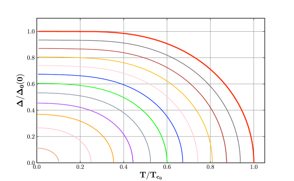
Figure 1: (Color online) Suppression of the B-phase order parameter in the unitary limit as a function of $\alpha=1/2\pi\tau T_{c_{0}}$. $\Delta(T)$ is normalized by $\Delta_{0}(0)=1.78k_{B}T_{c_{0}}$ for pure ³He-B in the weak-coupling limit (red curve). The curves for $0<\alpha\leq 0.275$ are shown for $\alpha$ in steps of $0.025$.

For the B-phase, $|\bm{\Delta}(\hat{\bf p})|^{2}=|\Delta|^{2}$ is isotropic, the angular integration over the Fermi surface is trivial and we can solve the gap equation numerically to obtain the magnitude of the order parameter. Figure 1 shows the de-pairing effect on both the transition temperature and the magnitude of the order parameter over the full temperature range as a function of $\alpha$ for unitary scattering.

The free energy functional for spatially uniform phases of ³He-aerogel is obtained by carrying out the integration in Eq. (Free Energy Functional) over the impurity renormalized propagator in Eq. (15). For unitary spin-triplet states and impurity scattering in the unitary scattering limit we obtain,

$$\Delta\bar{\Omega}\bigl{[}\bm{\Delta},\bm{\Delta}^{*}\bigr{]} = N_{f}V\,\Bigg{\langle}-\frac{1}{v_{1}}\,|\bm{\Delta}(\hat{\bf p})|^{2}+2\pi T\sum_{\epsilon_{n}}^{\prime}\Big{[}\left(|\widetilde{\epsilon}_{n}|-\sqrt{\widetilde{\epsilon}_{n}^{2}+|\bm{\Delta}(\hat{\bf p})|^{2}}\right)$$ (20)

$$\qquad\times\left(1+\frac{1}{2\tau|\widetilde{\epsilon}_{n}|}\right)+\frac{1}{2\tau}\ln\left(\frac{\sqrt{\widetilde{\epsilon}_{n}^{2}+|\bm{\Delta}(\hat{\bf p})|^{2}}}{|\widetilde{\epsilon}_{n}|}\right)\Big{]}\Bigg{\rangle}_{\hat{\bf p}}\,,$$

$$\widetilde{\epsilon}_{n} = \epsilon_{n}+\Bigg{\langle}\frac{1}{2\tau}\frac{\sqrt{\widetilde{\epsilon}_{n}^{2}+|\bm{\Delta}(\hat{\bf p})|^{2}}}{\widetilde{\epsilon}_{n}}\Bigg{\rangle}_{\hat{\bf p}}\,.$$ (21)

This functional reduces to the weak-coupling functional for pure ³He (Eq. 5.16 of Ref. Serene and Rainer (1983)) for $\tau\rightarrow\infty$. One can also verify that the stationarity condition for the ensemble averaged functional, $\delta\Delta\bar{\Omega}/\delta\bm{\Delta}(\hat{\bf p})^{*}=0$, generates the impurity renormalized gap equation, i.e. Eq. (17).

The thermodynamic potential, entropy and heat capacity of BW phase with homogeneous, isotropic disorder are obtained by evaluating the ensemble averaged free energy functional with the self-consistently determined solutions of Eqs. (18), (20) and (21).

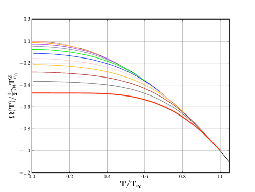
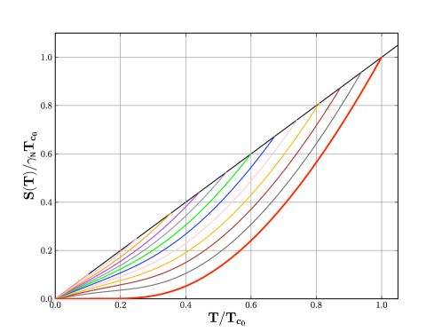
Figure 2: (Color online) Thermodynamic potential (left panel) and entropy (right panel) for the B-phase of ³He-aerogel in the unitary limit as a function of $T/T_{c_{0}}$ for pair breaking ranging from $0\leq\alpha\leq 0.275$ in steps of $0.025$. Results for pure ³He-B are shown as red curves.

Thermodynamic Functions

Figure 2 shows the thermodynamic potential (left panel) and entropy (right panel) for the dirty B-phase for values of the pair breaking parameter spanning the range from weak to strong pair breaking. Note that we plot the full thermodynamic potential, $\Omega_{\mbox{\tiny S}}(T)=\Omega_{\mbox{\tiny N}}(T)+\Delta\bar{\Omega}(T)$, which includes the normal-state contribution $\Omega_{\mbox{\tiny N}}(T)=-\frac{\mbox{\footnotesize 1}}{\mbox{\footnotesize 2}}\gamma_{\mbox{\tiny N}}\,T^{2}$, and we normalized the potential in units of $\frac{\mbox{\footnotesize 1}}{\mbox{\footnotesize 2}}\gamma_{\mbox{\tiny N}}\,T_{c_{0}}^{2}$, where $\gamma_{\mbox{\tiny N}}=\frac{\mbox{\footnotesize 2}}{\mbox{\footnotesize 3}}\pi^{2}N_{f}$ is the Sommerfeld coefficient for the normal state. The entropy was computed by numerically differentiating the thermodynamic potential, $S(T)=-\partial\Omega/\partial T|_{\mbox{\tiny V}}$. For pure ³He-B the entropy vanishes exponentially for $T\ll T_{c_{0}}$, but for the disordered B-phase in the unitary limit the entropy vanishes linearly for sufficiently low temperatures, $S(T)\rightarrow\gamma_{\mbox{\tiny S}}T$, where $\gamma_{\mbox{\tiny S}}$ is the Sommerfeld coefficient for the gapless B-phase. The gapless regime is achieved for $T\ll 0pt$, where $0pt\simeq\sqrt{\Delta(0)/2\tau}$ is the bandwidth of the impurity-induced excitation spectrum near the Fermi level.

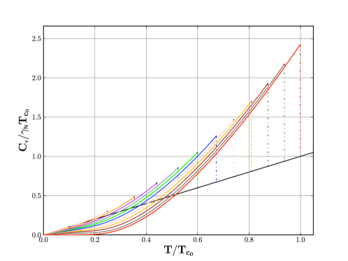
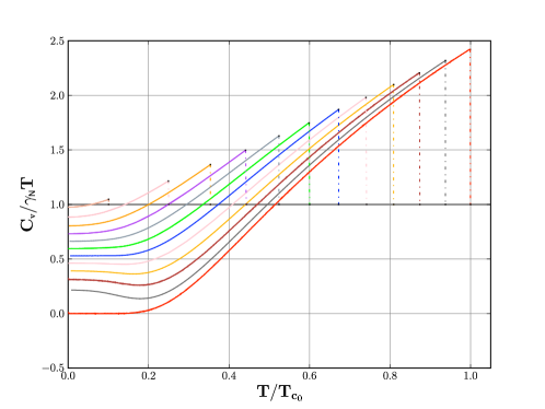
Figure 3: (Color online) Specific heat capacity normalized by $\gamma_{\mbox{\tiny N}}T_{c_{0}}$ (left panel) and by $\gamma_{\mbox{\tiny N}}T$ (right panel) for the B-phase of ³He-aerogel in the unitary limit as a function of $T/T_{c_{0}}$ for pair breaking ranging from $0\leq\alpha\leq 0.275$ in steps of $0.025$. Results for pure ³He-B are shown as red curves.

The heat capacity provides both a quantitative measure of the order that develops at $T_{c}$, as well as the spectrum of gapless states near the Fermi level. Figure 3 (left panel) shows results for the specific heat, $C_{\mbox{\tiny V}}=T\partial S/\partial T|_{\mbox{\tiny V}}$ over the full temperature range. The reduction of the heat capacity jump at $T_{c}$ computed from the thermodynamic potential agrees with the value calculated from the GL theory of Ref. Thuneberg et al. (1998) to three significant figures for all values of the pair breaking parameter. The right panel is the same data for the heat capacity plotted as $C_{\mbox{\tiny V}}/\gamma_{\mbox{\tiny N}}T$ vs. $T/T_{c_{0}}$. For weak to modest pair-breaking, $\alpha=1/2\pi\tau T_{c_{0}}<0.1$, corresponding to $\ell_{\mbox{\tiny el}}>1600\,\mbox{\AA}$ at $p=33\,\mbox{bar}$, $C_{\mbox{\tiny V}}/T$ is a non-monotonic function of $T$, however the limiting low-temperature heat capacity is linear in temperature, $C_{\mbox{\tiny V}}\rightarrow\gamma_{\mbox{\tiny S}}T$, where $\gamma_{\mbox{\tiny S}}$ is the Sommerfeld coefficient for temperatures below the impurity bandwidth, $T\lesssim 0pt$. The non-monotonic behavior of $C_{\mbox{\tiny V}}/T$ for $\alpha\lesssim 0.1$ results from the gap between the impurity band and the continuum states with $\varepsilon\geq|\Delta|$ (see Fig. 4). The limiting value provides the Sommerfeld coefficient for the gapless B-phase, $\gamma_{\mbox{\tiny S}}=\gamma_{\mbox{\tiny N}}\lim_{T\rightarrow 0}C_{\mbox{\tiny V}}/\gamma_{\mbox{\tiny N}}T$. One can infer from the calculated Sommerfeld coefficient for the gapless B-phase the density of states at the Fermi level, i.e. $\gamma_{\mbox{\tiny S}}=\frac{\mbox{\footnotesize 2}}{\mbox{\footnotesize 3}}\pi^{2}\,N(0)$.

Density of States

On the other hand, the density of states can be calculated directly by analytic continuation of the Matsubara propagator to real energies,

$$\mathfrak{g}(i\epsilon_{n}) \xrightarrow[]{i\epsilon_{n}\rightarrow\varepsilon+i0^{+}} \mathfrak{g}^{R}(\varepsilon)=-\pi\frac{\widetilde{\varepsilon}^{R}(\varepsilon)}{\sqrt{|\Delta|^{2}-(\widetilde{\varepsilon}^{R}(\varepsilon))^{2}}}\,,$$ (22)

$$\widetilde{\epsilon}^{R} = \epsilon+i0^{+}-\frac{1}{2\tau}\frac{\sqrt{|\Delta|^{2}-(\widetilde{\epsilon}^{R}(\varepsilon))^{2}}}{\widetilde{\epsilon}^{R}}\,.$$ (23)

$$N(\varepsilon)=N_{f}\,\Bigg{(}-\frac{1}{\pi}\mathrm{Im}\,\mathfrak{g}^{R}(\varepsilon)\Bigg{)}\,,$$ (24)

where $N(\varepsilon)$ is the density of states (DOS) at excitation energy $\varepsilon$ measured relative to the Fermi level. Figure 4 shows the results for the DOS (left panel) from weak to strong pair breaking calculated in the unitary limit for $T\rightarrow 0$. Note that the excitation energy for each value of pairbreaking is normalized by the appropriate value of the order parameter, $\Delta(0)$. The divergence of $N(\varepsilon)$ at $\varepsilon=\pm|\Delta|$ is suppressed by impurity scattering, and gapless excitations are created near the Fermi level for any $\alpha\neq 0$ in the unitary scattering limit.

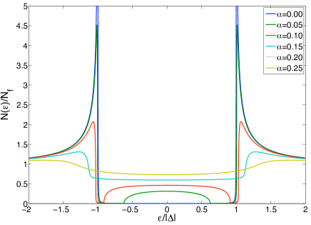
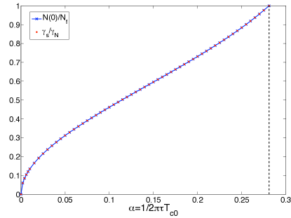
Figure 4: (Color online) Density of states as a function of excitation energy from weak to strong pair breaking (left). Comparison of the normalized density of states at the Fermi level (right panel), $N(0)/N_{f}$ obtained by direct calculation from Eq. (24), and the Sommerfeld ratio, $\gamma_{\mbox{\tiny S}}/\gamma_{\mbox{\tiny N}}$ computed from the limit, $\lim_{T\rightarrow 0}C_{\mbox{\tiny S}}/T$.

The normalized density of states at $\epsilon=0$ can be compared with that inferred from the calculated from the Sommerfeld coefficient. This provides a strong test of our calculations for the thermodynamic potential, entropy and heat capacity, as well as the validity of the ensemble averaged free energy functional obtained in Eq. (20). As Figure 4 shows the results for $N(0)/N_{f}$ and $\gamma_{\mbox{\tiny S}}/\gamma_{\mbox{\tiny N}}$ (right panel) are in perfect agreement. Note that $N(0)/N_{f}$ and $\gamma_{\mbox{\tiny S}}/\gamma_{\mbox{\tiny N}}$ vanish for $\alpha=0$ and both approach 1 continuously for $\alpha\rightarrow\alpha_{c}\approx 0.281$.

In summary we have obtained an ensemble averaged free energy functional for the superfluid ³He in in the presence of homogeneous, isotropic impurity disorder. This functional is based on a quasiclassical reduction of the Luttinger-Ward functional. Results for the thermodynamic potential, entropy and heat capacity were obtained by numerical evaluation of the stationarity conditions. The predicted Sommerfeld ratio based on the new functional agrees exactly with a direct calculation of the DOS from a solution of the quasiclassical transport equation. A quantitative comparison between theory and experimental measurements of the heat capacity of superfluid ³He-B in aerogel Choi et al. (2004) made at intermediate and high pressures will be discussed in a separate report.

References

- Halperin and Sauls (2004) W. P Halperin and J. A Sauls, arXiv, cond-mat.supr-con:0408593, 2004.
- Thuneberg et al. (1998) E. V. Thuneberg, et al. Phys. Rev. Lett., 80:2861, 1998.
- Sprague et al. (1996) D.T. Sprague, et al. Phys. Rev. Lett., 77:4568, 1996.
- Barker et al. (2000) B. I. Barker, et al. Phys. Rev. Lett., 85:2148, 2000.
- Sauls et al. (2005) J. A. Sauls, et al. Phys. Rev. B, 72(2):024507, 2005.
- Choi et al. (2004) H Choi, et al. Phys. Rev. Lett., 93(14):145301, 2004.
- Luttinger and Ward (1960) J.M. Luttinger and J.C. Ward. Phys. Rev., 118:1417, 1960.
- DeDominicus and Martin (1964) C. DeDominicus and P. Martin. J. Math. Phys., 5:14, 1964.
- Serene and Rainer (1983) J. W. Serene and D. Rainer. Phys. Rep., 101:221, 1983.
- Eilenberger (1968) G. Eilenberger. Zeit.f. Physik, 214:195, 1968.
- Choi and Muzikar (1989) C.H. Choi and P. Muzikar. Phys. Rev., B39:11296, 1989.
- Buchholtz and Zwicknagl (1981) L. J. Buchholtz and G. Zwicknagl. Phys. Rev., B23:5788, 1981.
- Eilenberger (1966) G. Eilenberger. Zeit.f. Physik, 190:142, 1966.
- Matsumoto et al. (1997) K. Matsumoto, et al. Phys. Rev. Lett., 79:253, 1997.