Hot Jupiters from Secular Planet–Planet Interactions

Abstract

About 25 per cent of ‘hot Jupiters’ (extrasolar Jovian-mass planets with close-in orbits) are actually orbiting counter to the spin direction of the star[2]. Perturbations from a distant binary star companion[3, 4] can produce high inclinations, but cannot explain orbits that are retrograde with respect to the total angular momentum of the system. Such orbits in a stellar context can be produced through secular (that is, long term) perturbations in hierarchical triple-star systems. Here we report a similar application to planetary bodies, including both the key octupole-order effects and tidal friction, and find that it can produce hot Jupiters in orbits that are retrograde with respect to the total angular momentum. With distant stellar mass perturbers such an outcome is not possible[3, 4]. With planetary perturbers the inner orbit’s angular momentum component parallel to the total angular momentum need not be constant[5]. In fact, as we show here, it can even change sign, leading to a retrograde orbit. A brief excursion to very high eccentricity during the chaotic evolution of the inner orbit can then lead to rapid capture, forming a retrograde hot Jupiter.

Center for Interdisciplinary Exploration and Research in Astrophysics (CIERA), Northwestern University, Evanston, IL 60208, USA

Despite many attempts[3, 4, 6, 7, 8, 9, 10, 11, 12], there is no model that can account for all the properties of the known hot Jupiter (HJ) systems. One model suggests that HJs formed far away from the star and slowly spiraled in, losing angular momentum and orbital energy to the protoplanetary disk[13, 14]. This “migration” process should produce planets with low orbital inclinations and eccentricities. However, many HJs are observed to be on orbits with high eccentricities, and misaligned with the spin direction of the star (as measured through the Rossiter–McLaughlin effect[15]) and some of these ($8$ out of $32$) even appear to be orbiting counter to the spin of the star. In a second model, secular perturbations from a distant binary star companion can produce increases in the eccentricity and inclination of a planetary orbit[16]. During the evolution to high eccentricity, tidal dissipation near pericenter can force the planet’s orbit to decay, potentially forming a misaligned HJ[3, 4]. Recently, secular chaos involving several planets has also been proposed as a way to form HJs on eccentric and misaligned orbits[12]. A different class of models to produce a tilted orbit is via planet–planet scattering[6], possibly combined with other perturbers and tidal friction[8]. In such models the initial configuration is a densly-packed system of planets and the final tilted orbit is a result of dynamical scattering among the planets, in contrast to the secular interactions we study here.

In our general treatment of secular interactions between two orbiting bodies we allow for the magnitude and orientation of both orbital angular momenta to change (see Figure 1). The outer body (here either a planet or a brown-dwarf) gravitationally perturbs the inner planet on time scales long compared to the orbital period (i.e., we consider the secular evolution of the system). We define the orientation of the inner orbit with respect to the invariable plane of the system (perpendicular to the total angular momentum): a prograde (retrograde) orbit has $i_{1}<90^{\circ}$ ($i_{1}>90^{\circ}$), where $i_{1}$ is the inclination of the inner orbit with respect to the total angular momentum vector. Note that the word “retrograde” is also used in the literature to indicate orbital motion counter to the stellar spin. The directly observed parameter is actually the projected angle between the spin axis of the star and the orbital angular momentum of a HJ. Our proposed mechanism can produce HJs that are “retrograde” both with respect to the stellar spin and with respect to the total angular momentum. By contrast, a distant stellar companion can only succeed in the former. See the online Supplementary Information for more details; henceforth we will use the term “retrograde” only to indicate an orbit with $i_{1}>90^{\circ}$ as define above.

We assume a hierarchical configuration, with the outer perturber on a much wider orbit than the inner one. In the secular approximation the orbits may change shape and orientation but the semi-major axes are strictly conserved in the absence of tidal dissipation[5, 17]. In particular, the Kozai-Lidov mechanism[18, 19, 20] produces large-amplitude oscillations of the eccentricity and inclination when the initial relative inclination between the inner and outer orbits is sufficiently large ( $40^{\circ}<i<140^{\circ}$).

We have derived the secular evolution equations to octupole order using Hamiltonian perturbation theory[21, 22, 5]. In contrast to previous derivations of “Kozai-type” evolution, our treatment allows for changes in the $z$-components of the orbital angular momenta (i.e., the components along the total angular momentum) $L_{{\rm z},1}$ and $L_{{\rm z},2}$ (see Supplementary Information). The octupole-order equations allow us to calculate the evolution of systems with more closely coupled orbits and with planetary-mass perturbers. The octupole-level terms can give rise to fluctuations in the eccentricity maxima to arbitrarily high values[5, 22], in contrast to the regular evolution in the quadrupole potential[3, 4, 20], where the amplitude of eccentricity oscillations is constant.

Many previous studies of secular perturbations in hierarchical triples considered a stellar-mass perturber, for which $L_{\rm z,1}$ is very nearly constant[3, 4, 20]. Moreover, the assumption that $L_{\rm z,1}$ is constant has been built into previous derivations[23, 25]. However, this assumption is only valid as long as $L_{2}\gg L_{1}$, which is not the case in comparable-mass systems (e.g., with two planets). Unfortunately, an immediate consequence of this assumption is that an orbit that is prograde relative to the total angular momentum always remains prograde. Figure 1 shows the evolution of a representative system (here without tidal effects for simplicity): the inner planet oscillates between prograde and retrograde orbits (with respect to the total angular momentum) as angular momentum flows back and forth between the two orbits.

Previous calculations of planet migration through “Kozai cycles with tidal friction”[3, 4, 17, 20] produced a slow, gradual spiral-in of the inner planet. Instead, our treatment shows that the eccentricity can occasionally reach a much higher value than in the regular “Kozai cycles” calculated to quadrupole order. Thus, the pericenter distance will occasionally shrink on a short time scale (compared to the Kozai period), and the planet can then suddenly be tidally captured by the star. We propose to call this “Kozai capture.”

Kozai capture provides a new way to form HJs. If the capture happens after the inner orbit has flipped the HJ will appear in a retrograde orbit. This is illustrated in Figure 2. During the evolution of the system the inner orbit shrinks in steps (Fig. 2c) whenever the dissipation becomes significant, i.e., near unusually high eccentricity maxima. The inner orbit can then eventually become tidally circularized. This happens near the end of the evolution, on a very short time scale (see Fig. 2, right panels). In this final step, the inner orbit completely and quickly decouples from the outer perturber, and the orbital angular momenta then become constant. Therefore, the final semi-major axis for the HJ is $\approx 2r_{p}$, where $r_{p}$ is the pericenter distance at the beginning of the capture phase[26].

The same type of evolution shown in Figure 2 is seen with a broad range of initial conditions. There are two main routes to forming a HJ through the dynamical evolution of the systems we consider here. In the first, tidal friction slowly damps the growing eccentricity of the inner planet, resulting in circularized, prograde HJs. In the second, a sudden high-eccentricity spike in the orbital evolution of the inner planet is accompanied by a flip of its orbit. The planet is then quickly circularized into a retrograde short-period orbit. We can estimate the relative frequencies of these two types of outcomes using Monte Carlo simulations. Given the vast parameter space for initial conditions, a complete study of the statistics is beyond the scope of this Letter (but see Naoz et al., in preparation). However, we can provide a representative example: consider systems where the inner planet was formed in situ at $a_{1}=5\,$AU with zero obliquity (orbit in the stellar equatorial plane) and with some small eccentricity $e_{1}=0.01$, while the outer planet has $a_{2}=51\,$AU. The masses are $m_{1}=1\,M_{\rm J}$ and $m_{2}=3\,M_{\rm J}$. We draw the eccentricity of the outer orbit from a uniform distribution and the mutual inclination from a distribution uniform in $\cos i$ between $0$ and $1$ (i.e., isotropic among prograde orbits). For this case we find that, among all HJs that are formed, about $7\%$ are in truly retrograde motion (i.e., with respect to the total angular momentum) and about $50\%$ are orbiting counter to the stellar spin direction. Note that the latter fraction is significantly larger than what previous studies have obtained with stellar-mass perturbers (at most $\sim 10\%$ [3, 4]). The high observed incidence of planets orbiting counter to the stellar spin direction[2] may suggest that planet–planet secular interactions are an important part of their dynamical history.

Our mechanism requires that two coupled orbits start with a relatively high mutual inclination ($i>50^{\circ}$). The particular configuration in Figure 2 has a very wide outer orbit similar to those of directly imaged planets such as Fomalhaut b[27] and HR 8799b[28]. In this case the inner Jupiter could have formed in its original location in accordance with the standard core accretion model[29] on a nearly circular orbit. An alternative path to such a configuration involves strong planet–planet scattering in a closely packed initial system of several giant planets[8]. Independent of any particular planet formation mechanism, we predict that systems with misaligned HJs should also contain a much more distant massive planet or brown dwarf on an inclined orbit.

Figure 1: Dynamical evolution of a representative planet and brown dwarf system. Here we ignore tidal dissipation, but we do include the lowest-order post-Newtonian precession rate for the inner orbit. Here the star has mass $1\,M_{\odot}$, the planet $1\,M_{\rm J}$ and the outer brown dwarf $40\,M_{\rm J}$. The inner orbit has $a_{1}=6\,$AU and the outer orbit has $a_{2}=100\,$AU. The initial eccentricities are $e_{1}=0.001$ and $e_{2}=0.6$ and the initial relative inclination $i=65^{\circ}$. We show from top to bottom: (a) the inner orbit’s inclination ($i_{1}$); (b) the eccentricity of the inner orbit (as $1-e_{1}$); (c) and (d) the $z$-component of the inner- and outer-orbit’s angular momentum, normalized to the total angular momentum (where the $z$-axis is defined to be along the total angular momentum). The thin horizontal line in (a) marks the $90^{\circ}$ boundary, separating prograde and retrograde orbits. The initial mutual inclination of $65^{\circ}$ corresponds to an inner and outer inclination with respect to the total angular momentum (parallel to $z$) of $64.7^{\circ}$ and $0.3^{\circ}$, respectively. During the evolution, the eccentricity and inclination of the inner orbit oscillate, but, in contrast to what would be predicted from evolution equations truncated to quadrupole order [shown by the thin curves in panels (a) and (b)], the eccentricity of the inner orbit can occasionally reach extremely high values and its inclination can become higher then $90^{\circ}$. The outer orbit’s inclination always remains near its initial value. We note that more compact systems usually do not exhibit the same kind of regular oscillations between retrograde and prograde orbits illustrated here, as chaotic effects become more important and are revealed at octupole order (see Fig. 2). We find that $\sim 50\%$ of the time the inner orbit is retrograde.

Figure 2: Dynamical evolution of a representative two-planet system with tidal dissipation included. The inner planet becomes retrograde at 112 Myr, and remains retrograde after circularizing into a HJ. Here the star has mass $1\,M_{\odot}$, the inner planet $1\,M_{\rm J}$ and the outer planet $3\,M_{\rm J}$. The inner orbit has $a_{1}=6\,$AU and the outer orbit has $a_{2}=61\,$AU. The initial eccentricities are $e_{1}=0.01$ and $e_{2}=0.6$, the initial relative inclination $i=71.5^{\circ}$, and argument of periapsis is $45^{\circ}$. We show: (a) the inner orbit’s inclination ($i_{1}$); (b) the eccentricity of the inner orbit (as $1-e_{1}$); (c) the semi-major axis, peri-, and apo-center distances for the inner orbit and the peri- and apo-center distances for the outer orbit; (d) the magnitude of the angular momentum of the inner orbit; and, in (e) and (f) the $z$-components of the inner and outer orbit’s angular momenta, normalized to the total angular momentum. The initial mutual inclination of $71.5^{\circ}$ corresponds to inner- and outer-orbit inclinations of $64.7^{\circ}$ and $6.8^{\circ}$, respectively. During each excursion to very high eccentricity for the inner orbit [marked with vertical lines in panels (b) and (c)], tidal dissipation becomes significant. Eventually the inner planet is tidally captured by the star and its orbit becomes decoupled from the outer body. After this point the orbital angular momenta remain nearly constant. The final semi-major axis for the inner planet is $0.022\,$AU, typical for a HJ. The thin curves in panels (a),(b),(d),(e) and (f) show the evolution in the quadrupole approximation (but including tidal friction), demonstrating that the octupole-order effects lead to a qualitatively different behavior. For the tidal evolution in this example we assume tidal quality factors $Q_{\star}=5.5\times 10^{6}$ for the star and $Q_{\rm J}=5.8\times 10^{6}$ for the HJ (see Supplementary Information). We monitor the pericenter distance of the inner planet to ensure that it always remains outside the Roche limit[30]. Here, as in Figure 1, we also include the lowest-order post-Newtonian precession rate for the inner orbit.

We would like to thank Dan Fabrycky and Hagai Perets for discussions. SN acknowledges support from a Gruber Foundation Fellowship and from the National Post Doctoral Award Program for Advancing Women in Science (Weizmann Institute of Science). Simulations for this project were performed on the HPC cluster fugu funded by an NSF MRI award.

SN preformed a numerical calculations with some help from JT. All authors developed the mathematical model, discussed the physical interpretation of the results and jointly wrote the manuscript.

The authors declare that they have no competing financial interests.

Correspondence and requests for materials should be addressed to S.N
 (email: snaoz@northwestern.edu).

 

Supplementary Information

 

Octupole-order Evolution Equations and Angular Momentum Conservation

Our derivation corrects an error in previous Hamiltonian derivations of the secular evolution equations.

We consider a hierarchical triple system consisting of an inner binary ($m_{1}$ and $m_{2}$) and a third body ($m_{3}$) in a wider exterior orbit. We describe the system using canonical variables, known as Delaunay’s elements, which provide a particularly convenient dynamical description of our three-body system. The coordinates are chosen to be the mean anomalies, $l_{1}$ and $l_{2}$, the longitudes of ascending nodes, $h_{1}$ and $h_{2}$, and the arguments of periastron, $g_{1}$ and $g_{2}$, where subscripts $1,2$ denote the inner and outer orbits, respectively. Their conjugate momenta are:

$$L_{1} = \frac{m_{1}m_{2}}{m_{1}+m_{2}}\sqrt{k^{2}(m_{1}+m_{2})a_{1}}\ ,$$ (1)

$$L_{2} = \frac{m_{3}(m_{1}+m_{2})}{m_{1}+m_{2}+m_{3}}\sqrt{k^{2}(m_{1}+m_{2}+m_{3})a_{2}}\ ,$$

$$G_{1}=L_{1}\sqrt{1-e_{1}^{2}}\ ,\quad G_{2}=L_{2}\sqrt{1-e_{2}^{2}}\ ,$$ (2)

where $k^{2}$ is the gravitational constant, and

$$H_{1}=G_{1}\cos{i_{1}}\ ,\quad H_{2}=G_{2}\cos{i_{2}}\ ,$$ (3)

where $G_{1}$ and $G_{2}$ are the absolute values of the angular momentum vectors (${\bf G}_{1}$ and ${\bf G}_{2}$), and $H_{1}$ and $H_{2}$ are the z-components of these vectors.

We choose to work in a coordinate system where the total initial angular momentum of the system lies along the $z$ axis. The transformation to this coordinate system is known as the elimination of the nodes^30,17; the $x$-$y$ plane in this coordinate system is known as the invariable plane. Figure 3 shows the resulting configuration of the orbits. We obtain simple relations between $H_{1}$, $H_{2}$, $G_{1}$ and $G_{2}$, using ${\bf G}_{\mathrm{tot}}={\bf G}_{1}+{\bf G}_{2}$:

$$\cos{i} = \frac{G_{\mathrm{tot}}^{2}-G_{1}^{2}-G_{2}^{2}}{2G_{1}G_{2}}\ ,$$ (4)

$$H_{1} = \frac{G_{\mathrm{tot}}^{2}+G_{1}^{2}-G_{2}^{2}}{2G_{\mathrm{tot}}}\ ,$$ (5)

$$H_{2} = \frac{G_{\mathrm{tot}}^{2}+G_{2}^{2}-G_{1}^{2}}{2G_{\mathrm{tot}}}\ ,$$ (6)

where the relation for $H_{1}$ comes from setting ${\bf G}_{2}={\bf G}_{\mathrm{tot}}-{\bf G}_{1}$ (and similarly for $H_{2}$). Because total angular momentum is conserved by the evolution of the system, we must have ${\bf G}_{1}(t)+{\bf G}_{2}(t)={\bf G}_{\mathrm{tot}}=G_{\mathrm{tot}}\hat{z}$, implying that

$$h_{1}(t)=h_{2}(t)-\pi.$$ (7)

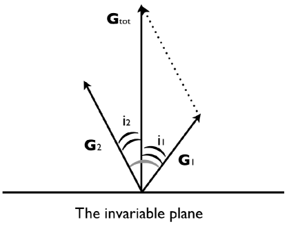
Figure 3: The angular momenta of the bodies after the elimination of the nodes (see also Ref. 4). Note that all three vectors are in the same plane. The mutual inclination $i=i_{1}+i_{2}$ is the angle between ${\bf G}_{1}$ and ${\bf G}_{2}$.

The Hamiltonian for the three-body system can be transformed into the form

$${\mathcal{H}}={\mathcal{H}}^{K}_{1}(L_{1})+{\mathcal{H}}^{K}_{2}(L_{2})+{\mathcal{H}}_{12},$$ (8)

where ${\mathcal{H}}^{K}_{1}$ and ${\mathcal{H}}^{K}_{2}$ represent the Keplerian interaction between bodies 1 and 2 and the central body, and ${\mathcal{H}}_{12}$ represents the interaction between body 1 and body 2. The Kepler Hamiltonians depend only on the momenta $L_{1}$ and $L_{2}$, while the interaction Hamiltonian, ${\mathcal{H}}_{12}$, depends on all the coordinates and momenta. Due to the rotational symmetry of the problem, ${\mathcal{H}}_{12}$ depends on $h_{1}$ and $h_{2}$ only through the combination $h_{1}-h_{2}$. Because we are interested in secular effects, we average the Hamiltonian over the coordinates (angles) $l_{1}$ and $l_{2}$, obtaining the secular Hamiltonian

$$\bar{{\mathcal{H}}}={\mathcal{H}}^{K}_{1}(L_{1})+{\mathcal{H}}^{K}_{2}(L_{2})+\bar{{\mathcal{H}}}_{12},$$ (9)

where

$$\bar{{\mathcal{H}}}_{12}=\frac{1}{4\pi^{2}}\int_{0}^{2\pi}dl_{1}\,\int_{0}^{2\pi}dl_{2}\,{\mathcal{H}}_{12}.$$ (10)

For simplicity we first focus on the quadrupole approximation, where the error is more easily shown; it is then straightforward to see its effects at all orders in the hierarchical triple system’s secular dynamics expansion. The quadrupole Hamiltonian results from expanding $\bar{{\mathcal{H}}}_{12}$ to second order in $a_{1}/a_{2}$:

$$\bar{{\mathcal{H}}}_{12}=\bar{{\mathcal{H}}}^{(2)}_{12}+{\mathcal{O}}\left(\frac{a_{1}}{a_{2}}\right)^{3}.$$ (11)

The resulting quadrupole-order Hamiltonian, $\bar{{\mathcal{H}}}^{(2)}_{12}$, depends only on the coordinates $g_{1}$, $h_{1}$, and $h_{2}$, with the latter two appearing only in the combination $h_{1}-h_{2}$:

$$\bar{{\mathcal{H}}}^{(2)}_{12}=\bar{{\mathcal{H}}}^{(2)}_{12}(g_{1},h_{1}-h_{2}).$$ (12)

Previous calculations^17,20 eliminated $h_{1}$ and $h_{2}$ from the Hamiltonian using eq. (7), obtaining a quadrupole Hamiltonian that depends only on $g_{1}$. But, this is incorrect! Such a Hamiltonian would imply that all quantities in eq. (5) are constant except $G_{1}$, i.e. that eq. (5) is incorrect. Thus the previously used formalism did not conserve angular momentum. The initial Hamiltonian is spherically symmetric, and therefore does conserve angular momentum; the correct quadrupole Hamiltonian does as well. Because the correct quadrupole Hamiltonian depends on $h_{1}$ and $h_{2}$ through the combination $h_{1}-h_{2}$, we have

$$\dot{H}_{1}=-\dot{H}_{2},$$ (13)

or

$$H_{1}+H_{2}=G_{\mathrm{tot}}={\rm const}.$$ (14)

The mathematical error affects all orders in secular perturbations. The independence of the secular quadrupole Hamiltonian on $h_{1,2}$ was the source¹⁷ of the famous relation $\cos i_{1,2}\sqrt{1-e_{1,2}^{2}}={\rm const}$. In the correct derivation, this relation does not always hold. However, in a certain limit, it does. From eq. (5), we see that

$$\dot{H}_{1}=\frac{G_{1}}{G_{\mathrm{tot}}}\dot{G}_{1}-\frac{G_{2}}{G_{\mathrm{tot}}}\dot{G}_{2}.$$ (15)

When $G_{2}\sim G_{\mathrm{tot}}\gg G_{1}$, we have

$$\dot{H}_{1}\approx-\frac{G_{2}}{G_{\mathrm{tot}}}\dot{G}_{2}.$$ (16)

At the quadrupole level $\bar{H}^{(2)}_{12}$ is independent of $g_{2}$, so $\dot{G}_{2}=0$, implying

$$\dot{H}_{1}\approx 0,$$ (17)

when $G_{2}\sim G_{\mathrm{tot}}\gg G_{1}$. This is precisely the limit considered in previous works^{2,3,17,18,19,31}, so their conclusion that $H_{1,2}=\cos i_{1,2}\sqrt{1-e_{1,2}^{2}}={\rm const}$ is correct (though not for the reason they claim), but the limit where $G_{2}\gg G_{1}$ is not sufficient for our work.

In some later studies, the assumption that $H_{1}={\rm const}$ was built into the calculations of secular evolution for various astrophysical systems^9,22-24, even when the condition $G_{2}\gg G_{1}$ was not satisfied. Moreover many previous studies simply set $i_{2}=0$, which is repeating the same error. In fact, given the mutual inclination $i$, the inner and outer inclinations $i_{1}$ and $i_{2}$ are set by the conservation of total angular momentum:

$$\cos i_{1} = \frac{G_{\mathrm{tot}}^{2}+G_{1}^{2}-G_{2}^{2}}{2G_{\mathrm{tot}}G_{1}}\ ,$$ (18)

$$\cos i_{2} = \frac{G_{\mathrm{tot}}^{2}+G_{2}^{2}-G_{1}^{2}}{2G_{\mathrm{tot}}G_{2}}\ .$$ (19)

Tidal Friction

We adopt the tidal evolution equations of Ref. 16, which are based on the equilibrium tide model of Ref. 32. The complete equations can be found in Ref. 2, eqs A1–A5. Following their approach (see their eq. A10) we set the tidal quality factors $Q_{1,2}\propto P_{\rm in}$ [see also Ref. 33]. This means that the viscous times of the star and planet remain constant; the representative values we adopt here are $5$ yr for the star and $1.5$ yr for the planet, which correspond to $Q_{\star}=5.5\times 10^{6}$ and $Q_{J}=5.8\times 10^{6}$, respectively, for a 1-day period.

Comparison to Observations

The observable parameter from the Rossiter–McLaughlin effect is the projected angle between the star’s spin and the orbital angular momentum (the projected obliquity)¹⁴. Here instead we focus on the true angle between the orbital angular momentum of the inner planet and the total angular momentum. Projection effects can cause these two quantities to differ in magnitude, or even sign.

Moreover, several mechanisms have been proposed in the literature that could, under certain assumptions, directly affect the spin axis of the star. These mechanisms can re-align the stellar spin axis through tidal interactions with either a slowly spinning star²⁹ or with the outer convective layer of a sufficiently cold star¹⁰. Additionally, a magnetic interaction between the star and the protoplanetary disk could also lead to misalignment between the stellar spin and the disk⁶.

These effects can potentially complicate the interpretation of any specific observation. Nevertheless, if hot Jupiters are produced by the simple mechanism described here, many of their orbits should indeed be observed with large projected obliquities.

References

- [1]
- [2] Triaud, A. H. M. J., et al. Spin-orbit angle measurements for six southern transiting planets. New insights into the dynamical origins of hot Jupiters. Astron. Astrophys. 524, A25 (2010).
- [3] Fabrycky, D. & Tremaine, S. Shrinking binary and planetary orbits by Kozai cycles with tidal friction. Astrophys. J. 669, 1298–1315 (2007).
- [4] Wu, Y., Murray, N. W. & Ramsahai, J. M. Hot Jupiters in binary star systems. Astrophys. J. 670, 820–825 (2007).
- [5] Ford, E. B., Kozinsky, B. & Rasio, F. A. Secular evolution of hierarchical triple star systems. Astrophys. J. 535, 385–401 (2000).
- [6] Chatterjee, S., Matsumura, S., Ford, E. B. & Rasio ,F. A. Dynamical outcomes of planet-planet scattering. Astrophys. J. 686, 580–602 (2008).
- [7] Lai, D., Foucart, F. & Lin, D. N. C. Evolution of spin direction of accreting magnetic protostars and spin-orbit misalignment in exoplanetary systems. Mon. Not. R. Astron. Soc. (submitted); preprint at http://arxiv.org/ abs/1008.3148, (2011).
- [8] Nagasawa, M., Ida, S. & Bessho, T. Formation of hot planets by a combination of planet scattering, tidal circularization, and the Kozai mechanism. Astrophys. J. 678, 498–508 (2008).
- [9] Schlaufman, K. C. Evidence of possible spin-orbit misalignment along the line of sight in transiting exoplanet systems. Astrophys. J. 719, 602–611 (2010).
- [10] Takeda, G., Kita, R. & Rasio, F. A. Planetary systems in binaries. I. Dynamical classification. Astrophys. J. 683, 1063–1075 (2008).
- [11] Winn, J. N., Fabrycky, D., Albrecht, S. & Johnson, J. A. Hot stars with hot Jupiters have high obliquities. Astrophys. J. 718, L145–L149 (2010).
- [12] Wu, Y. & Lithwick, Y. Secular chaos and the production of hot Jupiters. preprint at http://arxiv.org/abs/1012.3475 (2010).
- [13] Lin, D. N. C. & Papaloizou, J. On the tidal interaction between protoplanets and the protoplanetary disk. III - Orbital migration of protoplanets. Astrophys. J. 309, 846–857 (1986).
- [14] Masset, F. S. & Papaloizou, J. Runaway migration and the formation of hot Jupiters. Astrophys. J. 588, 494–508 (2003).
- [15] Gaudi, B. S. & Winn, J. N. Prospects for the characterization and confirmation of transiting exoplanets via the Rossiter-McLaughlin effect. Astrophys. J. 655, 550–563 (2007).
- [16] Holman, M., Touma, J. & Tremaine, S. Chaotic variations in the eccentricity of the planet orbiting 16 Cygni B. Nature 386, 254–256 (1997).
- [17] Eggleton, P. P., Kiseleva, L. G. & Hut P. The equilibrium tide model for tidal friction. Astrophys, J. 499, 853–870 (1998).
- [18] Kozai, Y. Secular perturbations of asteroids with high inclination and eccentricity. Astron, J. 67, 591–598 (1962).
- [19] Lidov, M. L. The evolution of orbits of artificial satellites of planets under the action of gravitational perturbations of external bodies. Planet. Space Sci. 9, 719–759 (1962).
- [20] Mazeh, T. & Shaham, J. The orbital evolution of close triple systems - The binary eccentricity. Astron. Astrophys. 77, 145–151 (1979).
- [21] Harrington, R. S. The stellar three-body problem. Celestial Mechanics 1, 200–209 (1969).
- [22] Krymolowski, Y. & Mazeh, T. Studies of multiple stellar systems - II. Second-order averaged Hamiltonian to follow long-term orbital modulations of hierarchical triple systems. Mon. Not. R. Astron. Soc. 304, 720–732 (1999).
- [23] Kiseleva, L. G., Eggleton, P. P. & Mikkola, S. Tidal friction in triple stars. Mon. Not. R. Astron. Soc. 300, 292–302 (1998).
- [24] Zdziarski, A. A., Wen, L. & Gierliński, M. The superorbital variability and triple nature of the X-ray source 4U 1820-303. Mon. Not. R. Astron. Soc. 377, 1006–1016 (2007).
- [25] Mikkola, S. & Tanikawa, K. Does Kozai resonance drive CH Cygni? Astron. J. 116, 444–450 (1998).
- [26] Ford, E. B. & Rasio, F. A. On the relation between hot Jupiters and the Roche limit. Astron. J. 638, L45–L48 (2006).
- [27] Kalas, P., et al. Optical images of an exosolar planet 25 light-years from Earth. Science 322, 1345–1348 (2008).
- [28] Marois, C., et al. Direct imaging of multiple planets orbiting the star HR 8799. Science 322, 1348–1352 (2008).
- [29] Pollack, J. B., et. al. Formation of the giant planets by concurrent accretion of solids and gas. Icarus 124, 62–85 (1996).
- [30] Matsumura, S., Peale, S. J. & Rasio, F. A. Formation and Evolution of Close-in Planets. Astrophys. J. 725, 1995–2016 (2010).
- [31] Jefferys, W. H. & Moser, J. Quasi-periodic solutions for the three-body problem. Astron. J. 71, 568–578 (1966).
- [32] Perets, H B. & Naoz, N. Tidal friction, and the dynamical evolution of binary minor planets. Astron. J. 699, L17–L21 (2009).
- [33] Hut, P. Tidal evolution in close binary systems. Astron. Astrophys 99, 126–140 (1981).
- [34] Hansen, P. Calibration of equilibrium tide theory for extrasolar planet systems. Astrophys. J. 723, 285–299 (2010).