Standing Slow-Mode Waves in Hot Coronal Loops:

Abstract

Strongly damped Doppler shift oscillations are observed frequently associated with flarelike events in hot coronal loops. In this paper, a review of the observed properties and the theoretical modeling is presented. Statistical measurements of physical parameters (period, decay time, and amplitude) have been obtained based on a large number of events observed by SOHO/SUMER and Yohkoh/BCS. Several pieces of evidence are found to support their interpretation in terms of the fundamental standing longitudinal slow mode. The high excitation rate of these oscillations in small- or micro-flares suggest that the slow mode waves are a natural response of the coronal plasma to impulsive heating in closed magnetic structure. The strong damping and the rapid excitation of the observed waves are two major aspects of the waves that are poorly understood, and are the main subject of theoretical modeling. The slow waves are found mainly damped by thermal conduction and viscosity in hot coronal loops. The mode coupling seems to play an important role in rapid excitation of the standing slow mode. Several seismology applications such as determination of the magnetic field, temperature, and density in coronal loops are demonstrated. Further, some open issues are discussed.

1 Introduction

The outermost layer of the Sun’s atmosphere, the corona, comprises of high temperature plasmas only visible in EUV and soft X-ray emissions, which reveal the highly inhomogeneous loop-like structures, believed to outline magnetic loops. Coronal loops are highly dynamic. Various periodic and quasi-periodic oscillations in radio, visible, EUV, and soft X-rays have been observed for decades (e.g. reviews by Aschwanden, 2003, 2004a; Wang, 2004; Banerjee et al., 2007). Most of these oscillations were interpreted as MHD waves. In particular, temporally and spatially resolved fast kink mode transverse oscillations and (both standing and propagating) slow mode longitudinal oscillations were credibly observed with TRACE satellite and SOHO spacecraft. These high resolution observations have turned MHD coronal seismology, originally suggested by Uchida (1970); Roberts et al. (1984), from a theoretical concept into a vibrant research area in solar physics (see reviews by Nakariakov & Verwichte, 2005; Wang, 2005; De Moortel, 2005; Ballester, 2007; Roberts, 2008). Measurements of wave properties (such as periods, amplitudes and damping times) and loop geometry in combination with theoretical modeling have been used to estimate physical parameters of coronal plasma such as magnetic field (Nakariakov & Ofman, 2001; Aschwanden et al., 2002; Wang et al., 2007), energy transport coefficients (Nakariakov et al., 1999; Ofman & Aschwanden, 2002), density stratification (e.g. Andries et al., 2005; Van Doorsselaere et al., 2008a), and loop temperature (Marsh et al., 2009; Wang et al., 2009b). MHD waves are also believed to play an important role in coronal dynamics (e.g., Nakariakov, 2007; Aschwanden, 2009) and coronal heating (e.g. Ofman et al., 1998; Aschwanden, 2004b; Nakariakov, 2004; Ofman, 2005; Taroyan & Erdélyi, 2009).

Global fast kink-mode transverse oscillations were first found in cool ($\sim$1 MK) coronal loops from TRACE EUV imaging observations (Aschwanden et al., 1999; Nakariakov et al., 1999). They were seen as spatial displacements with periods of 3$-$5 minutes and were apparently excited by flares or erupting filaments (Schrijver et al., 2002; Aschwanden et al., 2002). In several examples, the fundamental mode was found together with the second harmonic (or its first overtone) via time series analysis (Verwichte et al., 2004; Van Doorsselaere et al., 2007). A fundamental vertically polarized kink mode oscillation was first identified by Wang & Solanki (2004) using TRACE observations, and a fundamental horizontally polarized kink mode was recently identified by Verwichte et al. (2009) using STEREO/EUVI. Wang et al. (2008) found that for many combinations of viewing and loop geometry it is not straightforward to distinguish between these two types of kink modes just using time series of images. The combined fundamental horizontal and vertical kink mode oscillations are also possibly excited as suggested by TRACE and STEREO/EUVI observations (Wang et al., 2008; Aschwanden, 2009). In addition, the vertical kink oscillations were detected in coronal multithreaded loops with ejected cool plasma flows with the Hinode/SOT Ca ii H line filter (Ofman & Wang, 2008). The global fast kink mode oscillations were also observed with a 2D Doppler coronagraph working in the Fe xiv 5303Å line at the Norikura Solar Observatory (Hori et al., 2007). Various kinds of damping mechanisms have been proposed to explain the rapid decay of transverse oscillations observed by TRACE, among which resonant absorption (Ruderman & Roberts, 2002; Van Doorsselaere et al., 2004; Goossens, 2008), phase mixing (Nakariakov et al., 1999; Ofman & Aschwanden, 2002), and lateral wave leakage (Brady & Arber, 2005; Verwichte et al., 2006; Selwa et al., 2007a) are believed to be the most possible ones. In addition, recently some studies reported the discovery of Alfvén waves, such as ubiquitous waves in the corona detected in the time series of Doppler images (Tomczyk et al., 2007; Tomczyk & McIntosh, 2009), transverse waves in threadlike structure of solar prominences (Okamoto et al., 2007; Ning et al., 2009), and the transverse oscillation of spicules in the chromosphere (De Pontieu et al., 2007; He et al., 2009a, b). However, Van Doorsselaere et al. (2008b) suggested that these waves are more likely fast kink waves rather than the true (incompressible) Alfvén mode that is torsional in cylindrical plasma structure and hard to resolve by present instruments. These kink waves may be driven by solar $p$-modes (De Pontieu et al., 2005; Hindman & Jain, 2008; Tomczyk & McIntosh, 2009). Whether they decay during the travel has not been investigated in detail.

Propagating intensity disturbances were first detected in polar plumes with UVCS and EIT onboard SOHO (Ofman et al., 1997; DeForest & Gurman, 1998), and were interpreted as slow magnetoacoustic waves by Ofman et al. (1999, 2000). Their propagation, viscous dissipation, and refraction were studied by Ofman et al. (2000) using 2.5D MHD model. Subsequently, similar propagating disturbances along coronal loops were observed with SOHO/EIT (Berghmans & Clette, 1999) and TRACE (e.g. Nightingale et al., 1999; De Moortel et al., 2000). Their amplitudes are 3$-$4% and the propagating speed is on the order of 100 km s^-1 (De Moortel et al., 2002; McEwan & De Moortel, 2006). These upwardly propagating disturbances were also interpreted as the slow magnetoacoustic wave (Nakariakov et al., 2000). De Moortel et al. (2002) found that loops situated above sunspot umbras show oscillations close to 3 min, whereas non-sunspot loops (above plage regions) show oscillations close to 5 min. This close link between observed periodicity and location suggests that the waves are driven by the underlying $p$-modes oscillations (De Pontieu et al., 2005; De Moortel & Rosner, 2007; Hindman & Jain, 2008). Direct observational evidence for these waves propagating upwards along the magnetic field through the chromosphere and transition region into the lower corona have been found in both the cases of 3 minute oscillations (e.g. Brynildsen et al., 1999a, b; O’Shea et al., 2002; Marsh & Walsh, 2006) and 5 minute oscillations (Marsh et al., 2003; O’Shea et al., 2006; Wang et al., 2009a). However, Wang et al. (2009b) recently reported on observations of 12 and 25 min harmonics of similar propagating waves in coronal loops using Hinode/EIS observations. Since their periods are much longer than the cutoff period at the chromosphere and transition region, the origin of these waves are hardly explained by the wave leakage of the photospheric $p$-modes. In addition, Wang et al. (2009b) determined the plasma temperature near the footpoint region of loops using simultaneous measurements of intensity and Doppler shift oscillations. Marsh et al. (2009) obtained the temperature of the same order from observation of 3D propagation of similar waves with STEREO/EUVI. The rapid damping of these waves are mainly due to thermal conduction (De Moortel & Hood, 2003; Klimchuk et al., 2004). For a full review on propagating slow magnetoacoustic waves in coronal loops, readers can refer to De Moortel (2006, 2009). However, it should be noted that some recent studies argued that these propagating disturbances in fanlike loops and polar plumes observed with TRACE and EIT may not be the waves but likely quasi-periodically triggered upflows by episodic heating events based on the Hinode/EIS observations (Sakao et al., 2007; Harra et al., 2008; McIntosh & De Pontieu, 2009; McIntosh et al., 2010; He et al., 2010; De Pontieu & McIntosh, 2010). The detailed discussions are beyond the scope of this review.

Not only have the flare-excited transverse kink-mode oscillations but also the flare-excited longitudinal slow-mode oscillations have been observed in coronal loops. This review will focused on a discussion of the standing slow-mode waves in hot ($>$6 MK) loops observed by the SUMER spectrometer on SOHO, including the physical properties, their excitation and damping mechanisms, and some examples in coronal seismology. The SUMER Doppler shift oscillations will be compared with those observed by BCS onboard Yohkoh and recent results from EIS onboard Hinode. For the important role of standing slow mode waves in diagnostics of coronal heating, see a recent review by Taroyan & Erdélyi (2009).

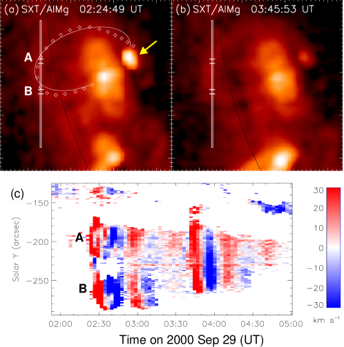
Figure 1: Observations of an oscillating hot coronal loop. (a) and (b) The Yohkoh/SXT images, showing that the Doppler-shift oscillation events may be triggered by microflares near a footpoint of the loop (marked with an arrow). (c) Doppler-shift time series in Fe xix observed with SOHO/SUMER in the sit-and-stare mode. Adapted from Wang et al. (2003b).

2 Properties of Observed Oscillations

2.1 Mode identification

The presence of slow mode oscillations in coronal loops was inferred by long-periodic (10$-$30 min) flux pulsations often seen in radio and X-ray wavelengths (Švestka, 1994; Aschwanden, 2003). Their first direct evidence was provided by Wang et al. (2002) using a high-resolution imaging spectrometer, SUMER, onboard SOHO. Strongly damped Doppler-shift oscillations show up in hot flare lines, Fe xix and Fe xxi, with formation temperature greater than 6 MK (Kliem et al., 2002; Wang et al., 2003a, b). Figure 1 shows an example, in which the coherent Doppler shift oscillations coincide with the regions where the slit crosses a hot loop seen in X-rays. Wang et al. (2002) analyzed two recurring events with coordinated SUMER and Yohkoh/SXT observations. From the measured loop length ($L\approx$140 Mm) and oscillation periods ($P$=14$-$18 min), they estimated the phase speed for the fundamental mode, $c_{t}=2L/P$=240$-$380 km s^-1, which are close to the sound speed at about 6 MK, thus suggesting an interpretation in terms of the standing fundamental slow mode. For seven oscillation events, Wang et al. (2007) derived the temperature of loops in the range of 6$-$7 MK and the electron density on the order of $10^{9}-10^{10}$ cm^-3 from the Yohkoh/SXT data. They estimated the period of the fundamental mode as $P\sim 2L/c_{s}$ where $c_{s}$ is the sound speed, and found the ratio of the predicted period to the measured period in the range 0.75$-$0.94, strongly supporting that the detected loop oscillations all belong to the fundamental slow mode. Wang et al. (2003b) measured physical parameters for 54 oscillation cases (Table 1) and found the oscillation periods in the range of 7$-$31 min with a mean of 17.6$\pm$5.4 min, which is distinctly larger than those (on average about 5 min) for the TRACE transverse oscillations (Aschwanden et al., 2002).

Table 1: Comparisons between physical properties of oscillations observed by SUMER (Wang et al., 2003b), Yohkoh/BCS (Mariska, 2006), and TRACE (Aschwanden et al., 2002; Ofman & Aschwanden, 2002).

Parameter	SUMER	BCS	TRACE
Oscillation period (minutes) ……..	17.6$\pm$5.4	5.5$\pm$2.7	5.4$\pm$2.3
Decay time (minutes)………………..	14.6$\pm$7.0	5.0$\pm$2.5	9.7$\pm$6.4
Amplitude (km s-1)………………….	98$\pm$75	17.$\pm$17.	42$\pm$53
Displacement (Mm)………………….	12.5$\pm$9.9	1.1$\pm$1.7	2.2$\pm$2.8
Decay time to period ratio………..	0.85$\pm$0.35	1.05$\pm$0.63	1.8$\pm$0.8

The interpretation of the SUMER oscillations as the standing slow mode is further supported by the evidence that the associated intensity variations show roughly a quarter-period phase delay to the Doppler signal in some cases (Wang et al., 2003a, b). Figure 2 shows one of the clearest examples. A quarter-period phase lag between velocity and intensity disturbances is a characteristic of the standing compressive wave. In contrast, the propagating wave shows an in-phase relationship (Sakurai et al., 2002).

In addition, the SUMER oscillations in the fundamental mode are also evidenced by the spatial distribution of Doppler shift amplitudes along the loop. Figure 3 shows a comparison of two brightening events observed by SUMER in the Fe xix line above a limb active region. The Doppler shift oscillations are clearly seen in the case when the slit is located at the loop top, whereas no oscillations but plasma flows are seen in the other case when the slit is located across the loop legs. The fact is consistent with the presence of an anti-node at the loop top in velocity perturbation for the fundamental slow mode.

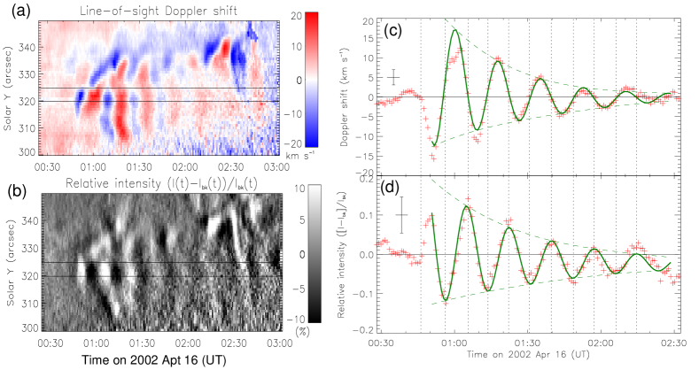
Figure 2: Observations of standing slow-mode waves in a flare loop with SUMER. (a) Time series of Doppler shift in Fe xix along the slit. (b) Time series of the relative intensity of Fe xix, normalized to the background emission. (c) and (d) Time profiles of average Doppler shift and relative intensity over a region along the slit marked in (a) and (b). The solid curves are the best fits with a damped sine function. The dashed curves are the fitted envelope.

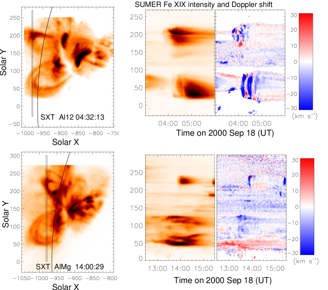
Figure 3: Comparison of two brightening events observed with Yohkoh/SXT (left panels) and SOHO/SUMER (middle and right panels). Upper panels: The case with the slit located at the loop apex. Bottom panels: the case with the slit located at the loop legs. Adapted from Wang et al. (2007). (Reproduced by permission of the AAS)

The detection of similar Doppler-shift oscillations during solar flares in emission lines of S xv and Ca xix with BCS on Yohkoh were reported by Mariska (2005). From measurements of 20 flares, Mariska (2006) obtained average oscillation periods of 5.5$\pm$2.7 min and decay times of 5.0$\pm$2.5 min . Comparison of the averages with the TRACE and SUMER results show that the BCS values are closer to those from TRACE than those from SUMER (Table 1). Since the BCS has no imaging capability, it is not possible to determine from the Doppler shift data alone whether the observed oscillations are the fast kink mode or slow mode. However, the existence of intensity fluctuations shifted by a quarter-period phase in some of flares argues strongly that all of the flare Doppler shift oscillations observed with BCS are slow-mode standing waves. In addition, this interpretation is also supported by the agreement between the loop length measured from SXT and the one derived from the observed wave period based on an assumption of the fundamental slow mode.

Therefore, it is most likely that the SUMER and BCS have observed the same phenomenon. Their difference in the period coverages may be caused by selective effects of the instruments. The temperature of hot oscillating loops observed by SUMER varies in the range about 6$-$8 MK as measured from the SXT data (Wang et al., 2007), whereas during the early phase of flares when the BCS oscillations are observed, the temperature measured in the S xv and Ca xix channels are high upto 12$-$14 MK (Mariska, 2006). Thus, the BCS tends to catch hotter loops which implies the higher phase speed, so the shorter wave period. The other reason (probably the major one) is that the BCS data often only extend for 20 min or less so that they prefer to detect the Doppler shift oscillations with the period less than 10 min (Mariska, 2006), while the SUMER data are mostly often acquired 50${}^{{}^{\prime\prime}}$$-$100${}^{{}^{\prime\prime}}$ off the limb, so prefer to detect oscillations of large loops with longer periods (Wang et al., 2003b).

For both the SUMER and BCS Doppler-shift oscillations only a few of cases are found to exhibit the intensity fluctuations with phase lags that are consistent with that expected for a standing slow mode wave. This may be explained by the spatial distribution of the amplitude in density perturbation along a loop for the fundamental mode, i.e. a node at the loop top and two antiphase antinodes at the footpoints. In the SUMER case, it is difficult to see intensity oscillations since the slit is located in most cases at the loop top (Wang et al., 2007), while in the BCS case one expects to see intensity oscillations only for the partially occulted flares since the BCS images the entire loop.

2.2 Triggers

Several pieces of evidence suggest that the SUMER Doppler shift oscillations are triggered by small (or micro-) flares near one footpoint of a coronal loop (Wang et al., 2003b). Firstly, all the SUMER oscillation events are only seen in hot flare lines of $T$$>$6 MK. Impulsive intensity time profiles and initial large line broadenings indicate the excitation of oscillations by impulsive heating. Of 27 SUMER flarelike events, Wang et al. (2003b) found that 4 were associated with the GOES C-class flares and 2 were the M-class flares. The others likely correspond to microflares with an X-ray flux below the detection threshold of GOES. Secondly, the SUMER oscillation events are characteristic of a high recurrence rate. More than half of the 27 events belong to recurring events (with a rate of 2$-$3 times within a couple of hours), which happen at the same place and manifest identical periods and initial Doppler shifts of the same sign (and not associated with CMEs). Thirdly, the initiation of some events is found associated with the X-ray brightening of a footpoint of the oscillating loop seen with Yohkoh/SXT and RHESSI. A survey of the SUMER oscillation events with RHESSI data have revealed that a dozen of the events were triggered by small flares with a hard X-ray source near footpoints of coronal loops (Wang et al. 2010, in preparation). Fourthly, the initiation of the SUMER events is found associated with a high-speed hot transient flow in coronal loops. Wang et al. (2005) examined the evolution of Fe xix and Fe xxi line profiles in the initial phase for 54 oscillations, and found that the nearly half show the presence of two spectral components. The shifted component reaches a maximum Doppler velocity on the order of 100$-$300 km s^-1. This feature indicates that the initial Doppler shifts are most likely caused by a pulse of hot plasma flowing along the loop.

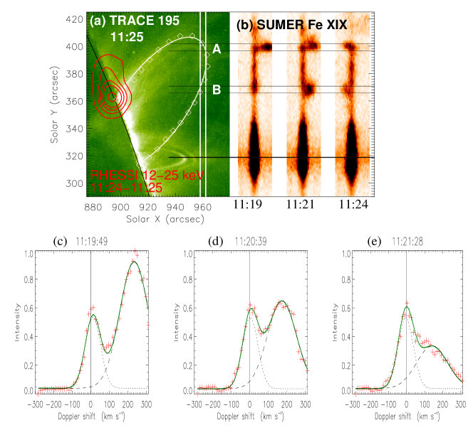
Figure 4: Observations of a hot loop oscillation event at the initial phase. (a) TRACE 195 Å image superimposed with RHESSI CLEAN image contours at 12-25 keV. (b) The SUMER Fe xix spectra along the slit. (c)-(e) Evolution of the Fe xix line profiles for position A marked in (b). The dotted and dashed curves are the fitted Gaussian functions to the two components: one representing the undisturbed loop emission, the other the injected high-speed flow emission. Adapted from Wang et al. (2005).

The features described above suggest a scenario for the trigger of SUMER oscillation events as follows. Small flares are triggered by a sudden energy release due to interactions (local magnetic reconnection) between two magnetic flux systems (e.g., a pre-existing large loop and a small twisted emerging loop), which produce so-called “confined flares” with no substantial change of the magnetic structure (and in particular no opening of the closed field system) (Heyvaerts et al., 1977; Démoulin et al., 1997; Karpen et al., 1998; Wang et al., 1999). The observed initial high-speed upflow is consistent with the impulsive chromospheric evaporation produced in flares (e.g. Fisher et al., 1985; Doschek & Warren, 2005; Milligan & Dennis, 2009), while the standing slow mode waves in flare loops are excited by a shock front or blast compression disturbance preceding the initial hot plasma flow.

Figure 1 shows a good example supporting this picture. In this example, two recurring oscillation events are associated with a footpoint brightening and both events begin with the redshifts (Wang et al., 2003b), suggesting that the events are triggered by an impulsive energy release near the footpoint of the oscillatory loop, while the initial redshifts are produced by hot evaporation (or reconnection) flows. Figure 4 demonstrates another clear example. This event initiates as two brightenings separated by a time lag and located near positions where the slit intersects a coronal loop. RHESSI observations show a hard X-ray source located at a footpoint of the loop, suggesting that a flare near the footpoint produces the high-speed hot flow and excites the slow mode oscillations in the loop. The evolution of spectral profiles shows that the oscillation set up immediately after the decay of the initial hot flow with a speed more than 200 km s^-1 (Wang et al., 2005).

The slow-mode oscillations observed by SUMER and BCS both appear to show a high excitation rate by small flares. Wang et al. (2006) studied the frequency distribution of thermal energy for small flarelike brightenings observed with SUMER in Fe xix above active regions on the limb. These brightenings have lifetimes ranging from 5 to 150 min with an average of about 25 min, and their estimated thermal energy from 10²⁶ to 10²⁹ erg with a power law index of 1.7 to 1.8. The features are well consistent with soft X-ray active region transient brightenings observed by Yohkoh/SXT (Shimizu, 1995), suggesting that these Fe xix brightenings are the coronal parts of loops heated to more than 6 MK by soft X-ray microflares. For nearly 300 events identified visually, 40% of them are associated with Doppler shift oscillations. Those events without showing evident oscillations may be ascribed to their observed location not close to the loop top (e.g., see Fig. 3). Mariska (2006) examined 103 flares observed by Yohkoh/BCS and found 38 showing oscillatory behavior in the measured Doppler shifts. Particularly, 20 of them with well-defined oscillations are mostly located at the limb. This location preference may be caused by the projection effect. As the longitudinal velocity perturbation (parallel to the field) has the maximum amplitude at the loop top for the fundamental mode, it tends to produce smaller Doppler-shift signals when a flare occurs in the loops located close to the disk center. This implies that the BCS Doppler-shift oscillations may be excited indeed more frequently than the observed. In addition, as the SUMER oscillations the BCS oscillations also prefer to be triggered by small flares. Of 20 events studied by Mariska (2006), 75% are C-class flares (the rest are M-class).

In summary, the above discussions suggest that standing slow mode oscillations are a nature of the confined flares, i.e. they are commonly excited by impulsive energy release in non-eruptive closed magnetic structure. Their property of the high excitation and occurrence rates make it invaluable for coronal seismology (see Sect. 4).

3 Theoretical Modeling

3.1 Excitation

For modeling the excitation of slow mode standing waves in hot loops observed by SUMER, Wang et al. (2005) suggested that consideration of the following observed properties are important.
1. The standing slow-mode waves in flaring loops are set up within one wave period.
2. The oscillations are the fundamental mode which appears to be triggered by impulsive asymmetric heating at one footpoint of the loop. The heating time is less than about half of the wave period, as implied by the duration of initial line width broadenings.
3. The loop plasma is impulsively heated to above 6 MK in the initial phase of events, and then gradually cools back to the initial temperature of about 2$-$3 MK.

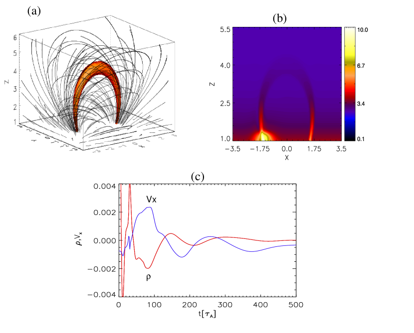
Figure 5: 3D MHD simulation of slow standing waves in a curved active region loop. (a) Initial 3D magnetic configuration of the model AR with a high density loop. (b) Mass density profiles in x-z plane (for y =0) at the beginning of simulation, when the pulse appears. (c) Time-signatures of the mass density and x-component of velocity at the loop’s apex. Adapted from Selwa & Ofman (2009).

The excitation of standing slow mode waves in hot coronal loops has been theoretically studied by many authors using 1D, 2D and 3D MHD models. In the 1D loop model, the magnetic field plays only a role to guide the wave. The advantage is that highly complex field-aligned energy transport processes can be accurately described using a full energy equation. Selwa et al. (2005) showed that pressure pulses launched close to a footpoint excite the fundamental mode, but forming the standing waves needs a dozen or so wave periods. Taroyan et al. (2005) analytically studied the excitation condition for the fundamental mode by the footpoint heating and found that to rapidly set up a standing wave in a single period it needs the duration of the heating pulse approximately matches the period of the oscillations. Under this assumption, Taroyan et al. (2007) studied a SUMER oscillation event using the forward modeling method. They estimated the duration, temporal behavior, and total heat input of the microflare and recovered the time-distance profile of the heating rate along the loop. Based on simulations of the similar model, Taroyan & Bradshaw (2008) predicted footprints and observables of standing and propagating acoustic waves in Hinode/EIS data. Patsourakos & Klimchuk (2006) also generated the synthetic line profile observations based on simulations of the loop oscillation produced by impulsive heating.

However, the duration of the heating pulse required to excite the standing wave in Taroyan et al. (2007) is too long to be supported by observations. This issue may come from the simple treatment of an actual 3D curved loop to the 1D model. Ogrodowczyk & Murawski (2007) showed that slow waves are excited faster in 2D straight slab than in a 1D loop due to coupling between the fast and slow magnetoacoustic waves. Selwa et al. (2007b) considered a 2D arcade loop model and found that the curved configuration plays an important role in efficient excitation of a slow standing wave because of the combined effect of the pulse inside and outside the loop. The standing wave can be set up within 1.6 wave periods. Ogrodowczyk et al. (2009) performed a parametric study using the similar 2D model. Recently, Selwa & Ofman (2009) extended the 2D arcade model to the 3D loop model in a dipolar field. Figure 5 shows that a velocity pulse covering both the footpoint of the loop and surrounding plasma can excite the standing fundamental mode of slow waves within a time interval comparable to the observations. The key point of the 2D and 3D models different from the 1D model is that a fast-mode component of the initial pulse is allowed to propagate quickly outside the loop and excites another slow pulse at the opposite footpoint almost simultaneously as the initial slow pulse (with respect to the time scale of the slow wave period). This effect may cause a great reduction in the excitation time of the standing wave. Pascoe et al. (2009) also studied impulsively generated oscillations in a 3D coronal loop, and found that a fundamental slow mode wave is excited when a pressure pulse nearby impacts on the loop almost parallel to the loop plane, but they did not mention the excitation time. Simulations of the excitation of standing slow waves in a 2D or 3D loop model by impulsive heating are required in the future for developing heating diagnostics of hot coronal loops with MHD waves.

In addition, Haynes et al. (2008) performed a 3D modeling of the kink instability in a twisted straight coronal flux tube, and found that the kink instability initially sets up the second harmonic that is then converted into two out-of-phase fundamental slow modes in two newly-formed, entwined structures. However, no evidence has been found that the SUMER oscillations are triggered by the kink instability.

Figure 6: Measured decay time vs. period for the events observed with the BCS reported by Mariska (2006), the SUMER events reported by (Wang et al., 2003b), and the TRACE events reported by Ofman & Aschwanden (2002), Wang & Solanki (2004), and Verwichte et al. (2004). The dashed line shows the best-fit to the BCS data, the dot-dashed line shows the fit to the SUMER data, and the solid line shows the fit to the combined BCS and SUMER data sets. Adapted from Mariska (2006). (Reproduced by permission of the AAS)

3.2 Damping

The Doppler shift oscillations observed by both SUMER and BCS decay strongly, with a ratio of the damping time to the period on the order of 1 (see Table 1). Figure 6 shows the decay time of the oscillations plotted against the period for the events observed with SUMER, BCS and TRACE. The fit to the combined SUMER and BCS data results corresponds to the expression $t_{decay}=1.30P^{0.81}$ (Mariska, 2006), which is very close to the fit to the SUMER data alone (Wang et al., 2003b).

Pandey & Dwivedi (2006) argued that the individual effect of thermal conduction or viscosity is not sufficient to explain the observed damping based on the linear analysis applicable for small amplitude waves. Sigalotti et al. (2007) compared the damping of standing slow waves due to various dissipation effects in both the linear and nonlinear regimes and obtained the similar conclusion. However, Ofman & Wang (2002) showed using nonlinear 1D MHD modeling that thermal conduction is the primary dissipation mechanism of the observed large amplitude standing slow-mode waves in hot coronal loops, and the scaling of the dissipation time with period agrees well with the SUMER oscillations. Mendoza-Briceño et al. (2004) showed that the damping times are reduced by 10$-$20% compared to homogeneous loops because of enhanced nonlinear viscous dissipation induced by gravity. Bradshaw & Erdélyi (2008) studied the effect of the radiative emission arising from a non-equilibrium ionization on the damping, and found that it may reduce the damping timescale by up to $\sim$10% compared to the equilibrium case. Haynes et al. (2008) showed that in the absence of thermal conduction, large-amplitude slow-mode oscillations are still damped rapidly due to shock dissipation. Verwichte et al. (2008) further studied the case in the presence of thermal conduction, and found that shock dissipation at large amplitudes enhances the damping rate by up to 50% above the rate given by thermal conduction alone. Erdélyi et al. (2008) studied the damping of standing slow waves in nonisothermal, hot, gravitationally stratified coronal loops, and found that the decay time of waves decreases with the increase of the initial temperature. They also derived a second-order scaling polynomial between the damping time and the parameter determining the apex temperature. Ogrodowczyk & Murawski (2007) found that standing slow waves are attenuated more efficiently in 2D straight slab than in 1D loop due to coupling between the fast and slow magnetoacoustic waves. Ogrodowczyk et al. (2009) further showed that these waves are attenuated more quickly in a curved 2D arcade than in a straight 2D slab configuration due to the possible enhanced wave leakage. Selwa & Ofman (2009) found that the damping of slow waves in the curved 3D loop is faster than in the curved 2D loop, and explained it in terms of lateral leakage because the 3D geometry provides additional degrees of freedom for the wave to leak out of the loop than 2D models. However, since these 2D and 3D MHD models metioned above do not include the dissipation terms such as thermal conduction and viscosity in the energy equation, it is unclear whether the coupling to the fast wave due to the transverse density inhomogeneity and the lateral leakage due to the loop curvature can dominate over the thermal conduction responsible for the rapid decay of observed standing slow-mode waves. This needs further investigation in the future.

4 Applications of Coronal Seismology

4.1 Determination of coronal magnetic field

Magnetic field plays a key role in understanding dynamics and heating of solar corona, however, direct measurement of the coronal magnetic field remains a very difficult problem. Recent high-resolution space observations have made MHD coronal seismology a promising tool to measure the coronal field indirectly. Table 2 shows many examples for estimates of the coronal field from the fast kink-mode oscillations in coronal loops. In contrast, Wang et al. (2007) determined the coronal field from the standing slow-mode oscillations in hot coronal loops observed by SUMER.

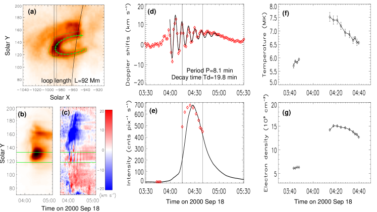
Figure 7: Coordinated observations of a hot loop oscillation event by SOHO/SUMER and Yohkoh/SXT. (a) The SXT image. (b,c) Line intensity and Doppler shift time series in Fe xix along the slit observed with SUMER. (d) Time profile of Doppler shifts averaged over a region marked in (c). The thick solid curve represents the best fit to a damped sine function. (e) Time profile of line intensities averaged over a region marked in (b). The superimposed data ($diamonds$) are the mean intensity of SXT emission averaged over an area at the loop top. (f,g) Temperature and electron density time profiles, calculated for the whole loop with the filter ratio method from SXT images. Adapted from Wang et al. (2007). (Reproduced by permission of the AAS)

The relative higher plasma $\beta$ in hot ($>6$ MK) loops implies the stronger coupling between magnetic perturbation and thermal perturbation than in the typical coronal structure, thus the magnetic field in hot loops may be deduced from diagnostics of standing slow-mode oscillations. Applying the MHD wave theory for a straight magnetic cylindrical model to the coronal loop (Edwin & Roberts, 1983), the oscillation period of a standing slow mode wave in its fundamental mode is given by,

$$P=\frac{2L}{c_{t}},\hskip 8.53581ptc_{t}=\left(\frac{1}{c_{s}^{2}}+\frac{1}{v_{A}^{2}}\right)^{-1/2},$$ (1)

where $L$ is the loop length, $c_{s}$ is the sound speed, and $v_{A}$ is the Alfvén speed. Roberts (2006) showed that the effect of gravitational stratification on the oscillation period of slow modes in hot SUMER loops is negligible. Erdélyi et al. (2008) showed that the effect of longitudinal temperature structure on the period is also trivial. Additional source of the uncertainty comes from the thin flux tube approximation of real coronal magnetic structure, under which the above expression is derived. From equation (1), the magnetic field can be derived as

$$B=\left(\frac{N_{e}}{C_{1}}\right)^{1/2}\left(\frac{P^{2}}{4L^{2}}-\frac{1}{C_{2}T}\right)^{-1/2},$$ (2)

where $C_{1}$ and $C_{2}$ are constants, $B$, $N_{e}$, and $T$ are the field strength, electron density, and loop temperature, respectively. For 7 Doppler-shift oscillation events simultaneously observed with the SUMER and Yohkoh/SXT, Wang et al. (2007) estimated the magnetic field in the range 21$-$61 G with a mean of 34$\pm$14 G. The subtraction of background emission leads to a reduction of the estimated values by 9%$-$35% (see Table 3). The error propagation analysis shows that the uncertainty in the estimated magnetic field is mainly contributed from uncertainties in temperature and loop length measurements which are reversely proportional to the plasma $\beta$. Figure 7 shows an example to demonstrate the measurements of $P$, $L$, $N_{e}$ and $T$. The period is measured by fitting the Doppler shift oscillations with a damped sine function. The loop length is measured by fitting the SXT loop with a simple geometric loop model. The average electron temperature and density are derived using the filter ratio method. Since $T$ and $N_{e}$ both evolved with time because of loop heating and cooling, their time-averaged values are used to determine $B$. Therefore, to improve the measurement accuracy of $B$, not only improved measurements of $T$ and $N_{e}$ should be conducted, but the effect of their temporal variations on the oscillation period also need to consider in the future.

Table 2: Overview of measurements of the coronal magnetic field from observations of fast kink-mode oscillations.

Reference	Wavelength	Instrument	$B$-field (G)	Loops
Nakariakov & Ofman (2001)…….	171 band	TRACE	4$-$30	2
Aschwanden et al. (2002)…………	171 & 195 bands	TRACE	3$-$90	26
Verwichte et al. (2004)…………….	171 band	TRACE	9$-$46	9
Ofman & Wang (2008)…………….	Ca II H band	Hinode/SOT	20$\pm$7	1
Van Doorsselaere et al. (2008c)…	Fe XII 195 line	Hinode/EIS	39$\pm$8	1
Erdélyi & Taroyan (2008)…………	Fe XII 195 line	Hinode/EIS	10$\pm$6	1
Verwichte et al. (2009)…………….	171 band	STEREO/EUVI	11$\pm$2	1

Table 3: Average and range of physical parameters for standing slow-mode oscillations in hot coronal loops measured from coordinated SUMER and Yohkoh/SXT observations. Adapted from Wang et al. (2007). (Reproduced by permission of the AAS)

Parameter	Before $I_{bk}^{\mathrm{a}}$ subtraction			After $I_{bk}$ subtraction
	Average	Range		Average	Range
Oscillation period $P$ (minutes) …….	11.2$\pm$3.8	8.1$-$18.3		Unchanged
Loop length $L$ (Mm) ………………….	116$\pm$44	74$-$199		Unchanged
Temperature $T$ (MK) …………………..	6.4$\pm$0.3	5.9$\pm$7.0		6.6$\pm$0.4	6.1$-$7.0
Electron density $N_{e}$ ($10^{9}$ cm-3) ……	8.4$\pm$3.6	4.3$\pm$14.1		7.4$\pm$3.3	3.4$-$12.4
Sound speed $c_{s}$ (km s-1) ………………	385$\pm$10	369$-$402		391$\pm$11	375$-$402
Alfvén speed $v_{A}$ (km s-1) …………..	830$\pm$223	442$-$1123		784$\pm$218	438$-$1123
Plasma $\beta$ …………………………………..	0.33$\pm$0.26	0.15$-$0.91		0.38$\pm$0.27	0.15$-$0.94
Magnetic field $B$ (G) …………………..	34$\pm$14	21$-$61		31$\pm$14	19$-$57

• $I_{bk}$ is the background emission of a loop.

4.2 Derivation of temperature evolution

We may explore temperature evolution of an oscillatory loop based on the relationship between the amplitudes of velocity and intensity variations for the slow mode wave. For a propagating wave, the amplitude relationship can be easily derived from the linearized continuity equation as $I^{\prime}/2I\sim\rho^{\prime}/\rho_{0}=V^{\prime}/c_{t}$, where $I^{\prime}/I$ and $V^{\prime}$ are the relative amplitude of the intensity and velocity amplitude, respectively, $\rho^{\prime}$ and $\rho_{0}$ are the density perturbation and the undisturbed loop density, and $c_{t}$ is the phase speed. As $\beta\ll{1}$ for a typical (T$\sim$1 MK) coronal loop, $c_{t}\approx{c_{s}}$. We thus can determine the sound speed (so the temperature) from the ratio between the intensity and velocity amplitudes (e.g. Wang et al., 2009b).

Figure 8: Time profile of Fe xix intensity (thin solid curve) observed by SUMER. The dashed curve is the 20-min window smoothing of the light curve. The thick solid line shows the cooling curve of loop temperature derived from the amplitude ratios between Doppler shift and relative intensity oscillations with Eq. (3).

For a standing wave the amplitude relationship also depends on the detected position of the oscillations. Wang et al. (2003a) derived it as,

$$\frac{I^{\prime}}{2I}\sim\frac{\rho^{\prime}}{\rho_{0}}=\frac{V_{x}}{c_{t}}|{\rm tan}(kx)|,$$ (3)

where $V_{x}=V^{\prime}{\rm cos}(kx)$, the amplitude of the detected oscillation at a position and $x$ is its distance to one footpoint along the loop. $k=\pi/L$, the wavenumber for the fundamental mode. For an event shown in Figure 2, Wang et al. (2003a) measured $x\approx 0.33L$ and the angle of $V_{x}$ to the line-of-sight, $\gamma$=15^∘, by fitting the loop geometry with a 3D circular model. The Doppler shift amplitude ($V_{\|}(t)$) and the relative intensity amplitude ($I^{\prime}(t)/I(t)$) are measured by fitting the oscillations with an exponentially damped sine function. We obtain that $V_{\|}(t)=18.3{\rm exp}(-t/33.7)$ km s^-1 and $I^{\prime}(t)/I(t)=0.16{\rm exp}(-t/43.6)$, where $t$ is in units of minute relative to the start time for fitting. So $V_{x}(t)=V_{\|}(t)/{\rm cos}\gamma$. From Eq. (1) it follows that $c_{t}=c_{s}/(1+\gamma\beta/2)^{1/2}$. Given $\beta$=0.3, a typical value for the SUMER hot loops (Wang et al., 2007), then $c_{t}=0.89c_{s}$. Finally, using Eq. (3) we obtain the loop temperature, $T(t)=9.2{\rm exp}(-t/74)$ MK. Figure 8 shows the derived temperature evolution from 00:51 to 02:28 UT, revealing that the loop cools from about 9.2 MK to 2.5 MK within a period of 86 min, over which the oscillations are clearly visible. This result agrees well with that measured in another event, where the SUMER slit is located at a similar height on the limb. The cooling time can be estimated as the delay time between the peak of the light curves seen in Ca xiii (3.2 MK) and Fe xix, which is about 90 min (see Fig. 11d). This example demonstrates that the method proposed above is reasonable.

The problem of the cooling of hot or post-flare loops was previously studied in both observation and theory by many authors (e.g. Antiochos & Sturrock, 1978; Antiochos, 1980; Culhane et al., 1994; Cargill et al., 1995; Harra-Murnion et al., 1998; Aschwanden & Alexander, 2001; Kamio et al., 2003). A well-accepted model by Cargill et al. (1995) assumes that conductive cooling initially dominates with radiative cooling taking over later on, suggesting that the cooling time of flaring loops can vary in a wide range depending on parameters such as the initial temperature, the loop length (or height) and the density. For example, from height$-$time curves of soft X-ray and H${\alpha}$ loops, Harra-Murnion et al. (1998) derived cooling times from 25 to 90 min for initial small and dense loops, while more than 100 min for later larger loops in an event using an initial temperature of 8 MK, which were found similar to the calculated cooling times using the method of Cargill et al. (1995). Our observations of the events discussed above unfortunately do not allow a comparison with the models because of the lack of density information although the measured cooling time appears to be in a reasonable range considering the large loop length ($\sim$200 Mm). The future observations from the combined Hinode/XRT, EIS and SDO/AIA will provide good opportunities in examining the seismological method suggested here in virtue of their abilities to simultaneously measure the temperature, density and geometry of the oscillating loop.

4.3 Diagnosis of plasma density

The Doppler shift oscillations observed by SUMER are strongly decayed, with a ratio of the damping time ($\tau_{d}$) to the period ($P$) on the order of 1 (Wang et al., 2003b). There are a few of cases, however, showing a peculiar weak decaying with oscillations visible for more than 5 periods and $\tau_{d}/P\geq 2$ (Wang et al., 2003a, 2007). Wang et al. (2003a) suggested that the weak damping may be due to a high plasma density in some flaring loops. This idea was confirmed by Pandey & Dwivedi (2006) based on the linear wave theory. They found that for coronal loops with a temperature in the range 6$-$10 MK, the strong-damped ($\tau_{d}/P$$\sim$1) oscillations occur in lower-density (10⁸$-$10⁹ cm^-3) loops, while the weak-damped ($\tau_{d}/P$$\geq$2) oscillations occur in higher-density (10⁹$-$10¹⁰ cm^-3) loops. This result appears to be supported by the coordinated SUMER and SXT observations. Figure 9 shows a comparison between the observed result and those predicted with and without including the effect of optically thin radiation besides thermal conduction and viscosity. We find that out of 7 loops, 4 seem to follow the curve predicted in the case when $T$=10 MK with the effects of thermal conduction and viscosity. This result suggests that the dependence of $\tau_{d}/P$ on $N_{e}$ and $T$ may be used to diagnose the density and temperature in oscillatory loops. However, given the huge error bars and marginal fit in Fig. 9, this will at best be an order of magnitude estimate in this example. Based on the future observations with Hinode/EIS and SDO/AIA, the validity of the method suggested here should be examined by comparing the derived plasma electron density and temperature with those obtained using the classic methods such as line intensity ratio and differential emission measure (DEM) techniques (e.g. Brosius et al., 1996; Landi et al., 2003).

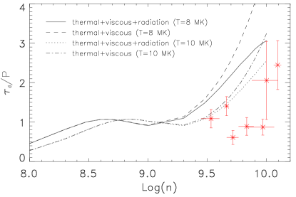
Figure 9: Variation of the ratio between the decay time and wave period ($\tau_{d}/P$) as a function of number density ($n$) for a loop length of 400 Mm. The solid and dashed curves correspond to a loop temperature of 8 MK, while the dotted and dash-dotted curves correspond to 10 MK (Adapted from Pandey & Dwivedi, 2006). The superimposed data are measurements from the SUMER and SXT observations reported by Wang et al. (2007).

5 Discussions

5.1 Propagating feature

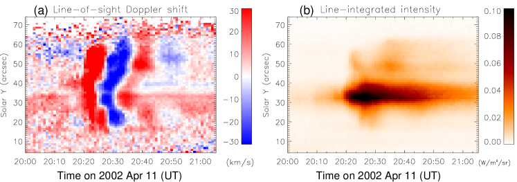
Figure 10: Propagation feature of Doppler shift oscillations revealed by high-cadence (50 s) SUMER observations. (a) Time series of Doppler shifts in Fe xix along the slit. (b) Time series of the Fe xix line intensity.

In some cases, high-cadence SUMER observations of Doppler oscillations exhibit the feature of phase propagation along the slit with speeds in the range 8$-$102 km s^-1 and a mean of 43$\pm$25 km s^-1. Figure 10 shows such an example. The phase delay seems to propagate along the slit from the strong emission region to the faint ones. This propagating feature apparently does not agree with the property of the fundamental standing waves, which should produce inphase oscillations along the loop. However, this feature is either inconsistent with that produced by propagating waves. Simulations by Taroyan & Bradshaw (2008) showed that the propagating slow-mode pulse reflecting back and forth inside the loop exhibits a triangle-like pattern in the time-distance plot of Doppler velocity. Hori et al. (2007) reported simultaneous excitation of transverse fast kink and longitudinal slow modes in a bundle of coronal loops. In the individual loops, a crossing diagonal pattern indicates the propagating slow waves reflecting on both ends of the loop. Instead, Wang et al. (2003b) proposed a scenario to explain the origin of this phase propagation by excitation of standing slow waves in coronal loops with the (multithreaded) fine structure. If magnetic reconnection triggers thermal energy release at a loop’s footpoint in a certain thread, the produced gas-pressure disturbance will affect the other threads at a slightly later time than the directly involved thread, thus exciting slow waves in those threads with phases delayed relative to the slow wave in the thread directly related to the trigger. The 3D MHD loop model in combination with the forward modeling method is necessary to test this idea.

5.2 Temperature dependence

The SUMER Doppler-shift oscillation events are all reported in hot flare lines, Fe xix and Fe xxi, with a formation temperature at above 6 MK (Wang et al., 2003b). Observations of these events at cooler lines have not yet been reported. It is not clear whether this implies that the excitation of slow mode standing waves requires the heating source with an energy input rate above certain threshold value, or only because the oscillations excited in loops heated to the lower temperature are too weak to be detected by SUMER. Recently, small amplitude (2$-$3 km s^-1) Doppler-shift oscillations are observed in Fe x$-$Fe xv lines with Hinode/EIS. Some are consistent with propagating slow magnetoacoustic waves, whose excitation appears to be related to the photospheric drivers (Wang et al., 2009a, b; Mariska & Muglach, 2010). While some others show evidence for standing slow-mode waves excited by small flarelike events (Mariska et al., 2008; Erdélyi & Taroyan, 2008). These oscillations have much smaller amplitudes than those of the SUMER oscillations that range from 12 to 353 km s^-1 with an average value of 62$\pm$57 km s^-1 (Wang et al., 2005). Mariska et al. (2008) found that the decay of the EIS oscillations shows an intriguing temperature dependence that the decay appears to be weaker seen in emission lines with the higher temperature of formation. This behavior is inconsistent with the the damping mechanism for standing slow mode waves by thermal conduction and compressive viscosity because they both cause the damping rate increasing with increasing temperature (Ofman & Wang, 2002). To figure out whether the oscillations in higher- and lower-temperature regimes have different physical properties and damping mechanisms first needs a reliable statistic study in the future.

On the other hand, recently some studies argued that those quasi-periodic propagating disturbances in large fanlike loops observed with TRACE and EIT may not be the true waves but the signature of episodic (or intermittent) heating events based on their association with tens of km s^-1 outflows observed at the edges of active regions with Hinode/EIS (Sakao et al., 2007; Harra et al., 2008; McIntosh & De Pontieu, 2009; He et al., 2010; De Pontieu & McIntosh, 2010). It is very important to verify whether these small-amplitude Doppler-shift oscillations observed with EIS are longitudinal waves or quasi-periodic, heating events for better understanding their physical properties.

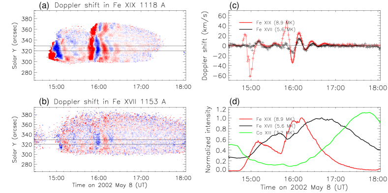
Figure 11: Simultaneous observations of hot loop oscillations in two emission lines by SUMER. (a) Time series of Doppler shift oscillation along the slit in Fe xix. (b) The Doppler shift oscillation in Fe xvii. (c) Time profiles of Doppler shift oscillations in Fe xix and Fe xvii averaged for a region marked in (a) and (b). The solid curves are the best fit to a damped sine function. (d) The corresponding average line intensities in Fe xix $\lambda$1118.06, Fe xvii $\lambda$1153.17 and Ca xiii $\lambda$1133.76.

In addition, the study of temporal dependence of wave properties on the temperature is another interesting topic, which is potentially applied in diagnostics of hydrodynamic processes related to impulsive heating of coronal loops. Figure 11 shows an example for Doppler-shift oscillation events observed simultaneously in Fe xix and Fe xvii lines with SUMER. The intensity evolution in Fe xix, Fe xvii and Ca xiii indicates a gradual cooling of the oscillating hot plasma in the loop (Fig. 11d). The initial amplitudes of oscillations seen in Fe xix are much larger than those in Fe xvii, while later on they tend to become consistency (Fig. 11c). The fitting to the second event (excluding the initial phase) shows that the period and decay time for the oscillations in the two lines are almost the same. This implies that the oscillations are produced by the same plasma and appear to decay quicker than the loop cooling. In other words, the decay of oscillations seen in Fe xix is real but not due to the cooling effect. Since the decay time (about 15 min) of oscillations in this event is shorter than the cooling time (about 30 min) of hot plasma seen in the emission from Fe xix to Fe xvii line, the oscillation has died out before the plasma cools to a lower temperature at which the oscillation is expected to have a longer decay time than that seen in Fe xix. Otherwise the oscillation seen in Fe xvii would last longer than in Fe xix.

5.3 Multiple harmonics

Multiple harmonics of coronal loop kink-mode oscillations have been detected by TRACE and applied to diagnose longitudinal structuring such as density stratification in coronal loops (e.g. Verwichte et al., 2004; Andries et al., 2009). For the slow mode several analytical studies showed that the longitudinal structuring or gravitational stratification can also modify the ratio between the period of the fundamental mode to that of the second harmonic strongly in certain conditions (Roberts, 2006; Díaz & Roberts, 2006; McEwan et al., 2006). For example, this ratio strongly departs from the canonical value of 2 in coronal loops with high density contrast between footpoints and apex or in cooler loops. Therefore, the detection of multiple harmonics is important in development of coronal seismology.

It was shown that Doppler-shift oscillations observed by SUMER in Fe xix and those observed by Yohkoh/BCS in S xv and Ca xix all appear to be consistent with the fundamental slow mode (Wang et al., 2003b, 2007; Mariska, 2006). Recently, Srivastava & Dwivedi (2010) stated that the evidence for multiple harmonics of slow acoustic oscillations was found in the nonflaring coronal loop with the Hinode/EIS data. However, the fact that the intensity signal with the period of the second harmonic is only detected at the loop apex but not at the footpoints does not completely agree with the theory.

Nakariakov et al. (2004) and Tsiklauri et al. (2004) simulated a high-temperature (20$-$30 MK) flaring loop using a 1D MHD model. They found that only the acoustic second standing harmonic is excited, regardless of the spatial position of heat deposition in the loop, and thus suggested that the quasi-periodic pulsations with periods in the range 10$-$300 s, frequently observed in flaring coronal loops in the radio, visible light and X-ray bands, may be produced by the second harmonic slow mode. However, direct evidence has not yet been found in observation. Nakariakov & Melnikov (2006) found that the fundamental and second harmonic modes have quite distinct observational signatures in the loop’s microwave images, which can be used to identify the mode in combination with analysis of the modulation frequency. In a different way, Selwa et al. (2005) numerically studied the excitation of standing slow-mode waves in a hot ($\sim$5 MK) coronal loop by launching a hot pulse at different positions. They found that pulses close to a footpoint excite the fundamental mode, while pulses close the apex excite the second harmonic. In some cases, observed is not a single mode but instead a packet of modes in which the fundamental and harmonic standing modes make the largest contribution. Thus, the interpretation of the SUMER oscillations in terms of the fundamental slow mode implies the possible asymmetric (footpoint) excitation, for which some pieces of evidence have been found in observations (see Sect. 2.2). In addition, it is noted that the wave decay rate of slow modes is larger for higher harmonics due to viscous damping or thermal conduction damping (Porter et al., 1994; Ofman et al., 2000). Thus, it is expected that detection of the higher harmonics is more difficult than the fundamental mode, especially in hot coronal loops.

6 Summary

The advance in observations and modelings of the standing slow mode waves have been reviewed in this paper. These strongly damped Doppler-shift oscillations are commonly observed in flaring hot coronal loops in active regions with different spectrometers such as the SUMER and BCS. The observed periodicities and the phase relationship between the Doppler shift and intensity variations indicate that they are fundamental standing slow-mode waves. The high excitation and recurrence rates of these oscillatory events in coronal loops suggest that the standing slow mode waves are a nature of confined (or non-eruptive) small- or micro-flares, which are produced by impulsive heating in closed magnetic structure. The theoretical studies show that the understanding of quick excitation of the fundamental mode needs at least the 2D MHD models with a curved geometry which allows the mode coupling to act, while the rapid damping can be well interpreted with the 1D nonlinear model.

Observations of the standing slow-mode oscillations in coronal loops are important for development of coronal seismology. The measured period has been applied to determine the mean magnetic field strength in coronal loops. The spatial and temporal relationship between Doppler shift and intensity oscillations may be used to diagnose the cooling of the flare plasma in coronal loops. In addition, the feature of phase propagation observed in Doppler shift oscillations by SUMER may have a potential to be used for diagnostics of fine structure of coronal loops based on 3D MHD modeling.

The Doppler-shift oscillations with small amplitudes of several km s^-1 were observed with Hinode/EIS in coronal loops of a temperature of 1$-$2 MK. These oscillations show a peculiar temperature-dependent behavior that the damping appears to be weaker seen in the higher temperature emission lines. The implication of this behavior is still unclear. So far, only the fundamental mode of slow mode oscillations is detected in hot flaring loops, although the excitation of the second harmonic is possible as predicted by numerical modeling with the symmetrical heating. The SDO/AIA with high spatio-temporal resolutions and wide (1$-$10 MK) temperature coverage will provide better statistics in identification of different (propagating or standing) oscillation modes and help elucidate the trigger sources and excitation conditions.