Redshift-space Enhancement of Line-of-Sight Baryon Acoustic Oscillations in the SDSS Main-Galaxy Sample
Abstract
We show that redshift-space distortions of galaxy correlations have a strong effect on correlation functions with distinct, localized features, like the signature of the baryon acoustic oscillations (BAO). Near the line of sight, the features become sharper as a result of redshift-space distortions. We demonstrate this effect by measuring the correlation function in Gaussian simulations and the Millennium Simulation. We also analyze the SDSS DR7 main-galaxy sample (MGS), splitting the sample into slices on the sky in various rotations. Measuring 2D correlation functions in each slice, we do see a sharp bump along the line of sight. Using Mexican-hat wavelets, we localize it to . Averaging only along the line of sight, we estimate its significance at a particular wavelet scale and location at 2.2. In a flat angular weighting in the coordinate system, the noise level is suppressed, pushing the bump’s significance to 4. We estimate that there is about a 0.2% chance of getting such a signal anywhere in the vicinity of the BAO scale from a power spectrum lacking a BAO feature. However, these estimates of the significances make some use of idealized Gaussian simulations, and thus are likely a bit optimistic.
Subject headings:
cosmology: large-scale structure of Universe - methods: data analysis1. Introduction
In a wide range of cosmological models, acoustic oscillations were generated due to competition between the pressure exerted by the photons and the gravitational collapse of perturbations in the density of baryons in the relativistic baryon-photon plasma of the early universe prior to the epoch of recombination (Silk, 1968; Peebles & Yu, 1970; Sunyaev & Zeldovich, 1970; Bond & Efstathiou, 1984, 1987; Holtzman, 1989). These are imprinted not only on the temperature power spectrum of the cosmic microwave background (CMB), as detected convincingly for the first time around the turn of the millennium (de Bernardis et al., 2000; Hanany et al., 2000), but also on the power spectrum of matter and galaxies. The Baryon Acoustic Oscillation (BAO) feature was first convincingly detected in the correlation function of Luminous Red Galaxies (LRGs) in the Sloan Digital Sky Survey (SDSS) by Eisenstein et al. (2005). Further evidence for the BAO has been found subsequently, in the SDSS and other galaxy surveys (Cole et al., 2005; Padmanabhan et al., 2007; Percival et al., 2007, 2010).
Some of these papers used correlation functions, others used power spectra. Correlation functions have both advantages and disadvantages over power spectra. For example, when there are quasi-harmonic features, like the BAO, forming a sequence of peaks in -space, they can add to a much stronger feature in the correlation function since the harmonics all add to the same peak in . A disadvantage of the correlation function is that unlike the power spectrum, it suffers from substantial off-diagonal covariances, even on large scales (e.g. Hamilton, 2009). However, it has recently been shown that even the power spectrum is not entirely immune from covariance effects in the mildly nonlinear regime (Rimes & Hamilton, 2005; Neyrinck et al., 2006).
Correlation functions of lower-dimensional subsets for a homogeneous isotropic random field are identical to the one estimated from the full three-dimensional one. This can also be extended to density fluctuations with line-of-sight anisotropies caused by redshift space distortions. Over the last two decades there were many redshift surveys, which had pencil-beam- or slice-like geometries (e.g. de Lapparent et al., 1988; Landy et al., 1996; Broadhurst et al., 1990; Pen et al., 2003; Weiner et al., 2005). Even wide angle surveys like the 2dF (Colless et al., 2001) had many pencil-beams as outrigger fields for a random sampling of a larger volume, while making optimal use of the multi-fiber capabilities of the telescope over a limited field of view. In any case, all these geometries should lead to the same redshift space correlation function. However, there are subtle effects due to the geometry entering the covariance of the correlation function.
The statistical analysis of significance for correlation functions is a notoriously difficult task (Kaiser & Peacock, 1991), since the different bins of the correlation function are always correlated to one another. The different modes in the power spectrum are more independent, as long as the survey window is large enough, making estimation in many ways easier (Tegmark et al., 1998). For anisotropic windows the shape of the independent “grains” in -space can be very elongated, leading to complications, like mixing modes over a wide range of scales. This is particularly true for pencil-beams or slices, where power spectra have rarely been used successfully to characterize structure.
Because the behavior of the BAO at low redshift only slightly departs from the predictions of linear cosmological perturbation theory, the BAO signature has recently attracted attention as a powerful “standard cosmological ruler.” It is a useful probe to explore the nature of dark energy or large-distance modifications of gravity, i.e. explanations of the observed accelerated expansion of the Universe.
There is a recent controversy about the reality of a narrow peak at the BAO scales along the line of sight (LOS) in the redshift-space power spectrum of the SDSS LRG sample (Gaztañaga et al., 2009). Gravitational lensing is mentioned as a possible origin of this signal, but this explanation has been disputed (Miralda-Escude, 2009). Kazin et al. (2010), using a suite of realistic LRG mock catalogs, conclude that the LOS peak is likely a statistical fluke. Recently, (Cabré & Gaztañaga, 2010) reached a similar conclusion about the significance of BAO detections, but argued that even a modestly significant peak can be used to constrain cosmological parameters, under the reasonable assumption that the galaxy power spectrum in the Universe contains a BAO feature.
In these papers, the statistical significance of a BAO feature is assessed by comparing data to models without BAO; for example, if a correlation function is better-fit by such a “no-wiggle” model, the features are judged to be spurious. Here, we test a different technique, detecting peaks with a Mexican-hat wavelet. Although it seems more forgiving of modest BAO-like peaks than the standard approach, we show that it still has much BAO-location constraining power
In this paper, we revisit the linear theory of redshift space distortions, and show that for power spectra with distinct spectral features, redshift space distortions will have a characteristic sharpening effect on these, especially along the line of sight, even in linear theory. In Section 2, we demonstrate how different geometric sampling strategies of a given survey volume can lead to strong, but quite different covariances in the resulting correlation functions. In Section 3, we describe our wavelet-based technique for BAO peak detection, and measure its statistical and systematic uncertainties using simple Gaussian simulations. In Section 4, we analyze a sample of galaxies from the Millennium simulation (MS Springel et al., 2005) using the wavelet technique. In Section 5, we build a sample of SDSS DR7 (Abazajian et al., 2009) main-galaxy sample galaxies, and analyze the LOS and 2D correlation functions using a methodology similar to the simulations: we subdivide the sample into many thin slices, compute the 2D redshift space correlation function and calculate the average. In Section 6, we apply the wavelet peak-finding formalism to the SDSS results. Finally, in the conclusion, we discuss our findings.
2. Redshift Space Correlations in Linear Theory
2.1. Amplifying the BAO Features
The seminal paper of Kaiser (1987) laid out the framework to compute the redshift space distortions of power spectra, in the plane-parallel limit, when the two galaxies are very close to the same LOS. Later, Hamilton (1992), and Hamilton & Culhane (1996) worked out explicit expressions for the correlation function. Heavens & Taylor (1995) considered the problem for all-sky redshift surveys using a spherical-harmonic analysis.
Szalay et al. (1998, hereafter SML98) used bipolar spherical harmonics to extend the previous calculations of the correlation function to arbitrary angles between the two lines of sight, and have computed explicit expressions for the distorted correlation function in different directions. Their work was further extended by Szapudi (2004) and Pápai & Szapudi (2008), using a slightly different coordinate system, and including contributions from a previously neglected term in the Jacobian of the real- to redshift-space mapping. Scoccimarro (2004) included various non-linear effects, in particular contributions from the nonlinear pairwise velocity distributions.
The basic papers laying out the theory of redshift-space distortions were written in the 80’s and 90’s, when the generally accepted assumption was that the cosmological dark matter power spectrum is smooth. Here we would like to show that one of the effects of the redshift space distortions on the correlation function is a sharpening of “bumpy” features, in directions close to the LOS.
Following SML98, we can write the redshift space correlation function as a function of the pairwise distance , and the angle ( in SML98), using the expression for the plane-parallel limit (especially applicable near the LOS), as
| (1) | |||||
where is the Legendre polynomial of order , is the usual redshift space distortion parameter, , where is the bias factor, and is the -th spherical Bessel transform of the isotropic, real-space power spectrum ,
| (2) |
The three-dimensional angular average of Eq. (1) is , using a weighting; only the isotropic contributes due to the orthogonality of the Legendre polynomials. However, such a weighting suppresses contributions from close to the LOS, where . If is averaged with a flat (without the factor) angular weighting, appropriate for a 2D sample, there are also contributions from and :
| (3) | |||||
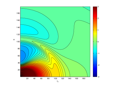
Figure 1 shows contours of the linear redshift-space correlation function derived from a power spectrum with a BAO bump at 107. In linear theory, the BAO feature sharpens near the LOS. Here and are galaxy separations projected parallel and perpendicular to the LOS. We use a transform for easy visualization for both large and small . The function equals for , and for .
The LOS correlation function, , can be written as
| (4) | |||||
The term independent of is just the isotropic, real-space correlation function. The term linear in can be written as , which inside the -integrals behaves as , the second derivative of the spherical Bessel function. Such operators were explicitly shown in Eq. (4) of Hamilton (1992). Applying a second derivative to a Gaussian, and adding it to the function with a positive weight will sharpen the peak, as seen in Fig. 2. The sharpening is much weaker far from the LOS, in the transverse () direction. The other effect of redshift-space compression is an overall smooth shift towards negative values along the LOS, and towards positive values in the transverse.

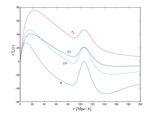
In Fig. 2, we also show the results if is multiplied by , in which case the peaks at different angles line up in scale more obviously. This could be because the slopes on which the peaks find themselves at different angles are much more similar in than in itself. This is an example illustrating how using the absolute position of ’s local maximum, without regard to the slope it is on, can produce a small bias. A peak locator that estimates the second derivative, as our wavelet transform does, is insensitive to such slopes.
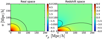
Fig. 3 shows an Eisenstein & Hu (1998) no-wiggle linear in real and redshift space. Note that the trough along the LOS at appears even in the no-wiggle case, and thus seems unrelated to the BAO feature in linear theory. However, as shown below in Fig. 21, the trough is highly amplified in samples with full nonlinearities (in the SDSS and MS samples); we suspect that this could be a result of non-linear infall toward the BAO ridge.
For every pair of galaxies, the observer and the two galaxies define a plane, and the whole problem is invariant under any rotation of this plane around the observer, located at the origin. Thus the anisotropic redshift space correlation function is inherently planar, and in 3D it has an axial symmetry for rotations around the LOS. This means that one can also estimate the same 2D correlation function from an arbitrarily thin slice of the data (though if one goes too thin, shot noise will swamp the signal). From the projection-slicing theorem, described below, this is equivalent to first projecting the three-dimensional redshift-space power spectrum down to two dimensions, and then perform a two-dimensional inverse Fourier transform. This has been noted in SML98. Computing the anisotropic redshift space correlation function this way does not violate any of the underlying symmetries of the problem. However, it impacts the covariances of the estimated correlation function, as we will show.
2.2. Projection-Slicing Theorem
There is well-known theorem in signal processing and medical imaging, stating a relation between the Fourier transform of a lower dimensional subset of a multidimensional scalar field and the original Fourier transform.
The projection-slicing theorem states that the Fourier transform of the projection of an -dimensional scalar function onto an -dimensional subspace is equal to an -dimensional slice, going through the origin of the -dimensional Fourier transform of . For example, if a 3D is projected to 2D along the direction, the Fourier transform of the 2D projection will be on the plane of the 3D Fourier transform of . Symbolically,
| (5) |
where denotes the -dimensional Fourier transform, denotes a projection onto the -dimensional subspace, and denotes slicing of the -dimensional subspace. This technique will be useful for the calculations below.
We can compute the redshift space correlation function in several different ways. We can take the full 3D redshift space correlation function, and perform the axial averaging using the LOS as the symmetry axis to get the 2D . Alternatively, we can compute the 2D correlation function directly from each slice in an ensemble, and then perform the averaging in 2D.
In the case of LOS correlations, one can do the either of the above procedures, then take the LOS, or one can even directly extract all possible pencil-beams from the volume and just compute the 1D correlation function. In the extreme, near the LOS, all three cases will contain the same galaxy pairs, nevertheless the covariances between the correlation function bins estimated in different ways will be somewhat different due to lateral correlations between neighboring slices and pencil-beams. In the following subsections we will illustrate how to compute the covariance of the correlation functions, at least in the linear limit, where the three results are quite intuitive, and show the subtle differences between the outcomes. Furthermore, even though the calculation below is only for the LOS correlation function, it can be easily extended for the covariance of the full 2D redshift space correlation function.
2.3. Estimating the covariance of from pencil-beams
We ignore the effects of shot noise, and only estimate the variance and covariance of the correlation function from the power spectrum. Consider first a single pencil-beam, aligned with the -axis, drawn randomly from a cubic volume with periodic boundary conditions, like the case of the N-body simulations we analyzed in this paper. The overdensity is measured in discrete cells, along each axis of the cube. The estimator for the LOS correlation function is
| (6) |
where is the dimensionless overdensity in the th cell along the LOS. The expectation value .
We can compute the expectation value
| (7) |
and the covariance
| (8) |
If we stay in the Gaussian (linear) limit, there are no higher order, irreducible contributions, thus the expectation value of the product of four overdensities can be factored as
| (9) |
With , we can write the expectation value as
| (10) | |||||
After the summation over the index , we obtain
| (11) |
The first term is just the trivial product of the expectation values. The next terms are the correlations of the correlation function, which we will denote as , a symmetric function of its argument, as
| (12) |
We can compute in the limit of infinitesimal cells, using the Fourier transform of the one dimensional , denoted as . Due to the projection-slicing theorem, the one-dimensional power spectrum corresponding to the correlation function along the pencil-beam is the projection of the three-dimensional power spectrum , anisotropic due to the redshift space distortions along the -axis:
| (13) |
and
| (14) |
In summary, we can write the covariance of the 1D correlation function as estimated from a single pencil-beam as
| (15) |
2.4. The covariance of for independent slices
Next, we randomly select a thin density slice from a cubic volume, and estimate the two dimensional correlation function. We essentially repeat the derivation above, except we have two indices: is along the LOS, and is along the slice:
| (16) |
The LOS correlation function is the special case with . Following the previous calculation, we obtain the equivalent 2D covariance as
| (17) |
with now related to , the 2D projection of the 3D power spectrum:
| (18) |
| (19) |
Along the LOS, can be written as:
| (20) |
This is the projection-slicing theorem at work again: we are ’slicing’ the 2D super-correlation function at , therefore, we need to project its power spectrum down to the -axis. This is however different from the previous result, there the projection has happened for the power spectrum, before the square was taken. Here we performed one projection before and one after taking the square of the power spectrum.
2.5. The covariance from the average of slices
We repeat the calculation of the LOS correlation function as above, but now we average over the whole three-dimensional cube. We can perform this by subdividing the volume into a set of adjacent slices, computing the correlation function of each slice, then averaging them over the whole set. The derivation is quite similar, except now we have a 3D estimator of the LOS correlation function. We will just present the final result:
| (21) |
| (22) |
with
| (23) |
Here all projection takes place after squaring the anisotropic 3D power spectrum. Even without evaluating any of the integrals one can see that the covariances will be the largest in this, third case, since the quadratic mean is always larger than the arithmetic one. So if at a given we project the square of the 3D power spectrum, we always get a larger number if some of the projection takes place before taking the square.
2.6. Effect of strong covariances on the estimated errors
We can write a linear transform of correlation function values in bins as , where are the coefficients of the linear transformation, and are the binned values of the 1D correlation function. Assuming that the transform has a finite support, the sum is over a small, finite number of bins. The expectation value of can be written as
| (24) |
For a wavelet transform, the vector contains some positive and negative coefficients, so that their sum is equal to 0. The expectation value of is
| (25) |
and the variance is
| (26) |
Consider a simple wavelet of length 3: . The covariance of the correlation function is dominated by the term. Since this is a symmetric function of its argument, it is reasonable to approximate it with an inverse parabola , taking also unit diagonal variance. Expanding the covariance matrix up to second order in
| (27) |
then the variance is given by . The covariances of the LOS correlation function are quite high. Thus, applying a similar, but much wider wavelet can potentially reduce the variance considerably compared to the nominal diagonal variances, although it will never go to zero as in this extreme example. This Section only serves as an illustration of the effect of the strong covariances, and the importance of the particulars of the sampling strategy chosen.
Let us describe what this means in simple terms. Consider first a set of independent, uncorrelated slices randomly drawn from a infinite sample, and denote the variance of a wavelet coefficient at some scale over this ensemble as . This variance will be already smaller than the variance of the individual bin values of the correlation function, since the covariance among the bins [] is reducing the wavelet variance.
Next, let us draw a set of adjacent slices from a coherent cubical volume, and compute the average wavelet coefficient over this sample. The covariance of the estimator now becomes much stronger, ; thus, the variance of the wavelet coefficient will be much smaller.
If we took the average over the same number of slices from the independent ensemble, the variance would be reduced by , due to the central limit theorem. For , though, estimating the variance among the slices assuming they are independent will be an underestimate of the true variance. But can be used as a definite bound on the expected variance reduction from the slice-averaging process. At the end of Section 5.4.1 we demonstrate this behavior using Gaussian simulations.
3. Quantifying the Redshift Space Features
3.1. Peak Location from a Mexican Hat Wavelet
We measure the sharpness of peaks in the correlation function using a Mexican hat wavelet, similar in spirit to the (differently shaped) wavelet technique proposed by Xu et al. (2010). A transform using a Mexican hat wavelet, a second derivative of a Gaussian, provides a measurement of (minus) the second derivative of a function, estimated over the scale radius of the wavelet. Before discussing the Mexican hat itself, we describe estimators of the zeroth and first derivatives of a function, also using derivatives of a Gaussian. These estimators will turn out to be useful in visualizing the sharpness of the BAO bump as a function of angle.
Define a Gaussian of scale radius , and normalized to equal 1 at its center (bump position ), as
| (28) |
(The arguments before the semicolon are really parameters of the function itself, which acts on parameters after the semicolon.) An estimate of the mean of (i.e. the zeroth derivative) within a radius of is given by the average . Here is the angle away from the LOS.
To estimate the radial first derivative within a radius of , we use the following, where :
| (29) |
| (30) |
We use to denote a generalized average: in the denominator, the terms multiplying in the integrand are squared.
An estimate of the second derivative is , with the Mexican hat wavelet,
| (31) |
The wavelet transform is given by
| (32) |
Numerically, what we do is to evaluate and integrate the numerator on the same grid as is measured, multiplying the integrand by to take out the weighting from the 2D integration. Note that whenever we use the transform, we divide means by standard deviations, so in fact the normalization (in the denominator) drops out.
We note that in practice, we analyze correlation functions that are undefined for , and while , . However, this problem is negligible if , and we confine our analysis to such cases.
3.2. Flattening transformation with background subtraction
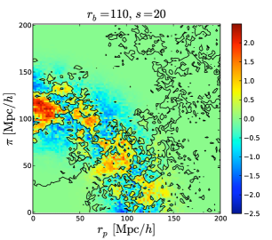
The redshift-space has a strong quadrupole anisotropy, making it difficult to see the strength of the peak at different angles. To make a visual detection of the peak easier, we flatten at a given radius by estimating, and then subtracting, the zeroth and first derivatives with respect to both radius and angle. This is the background subtracted correlation function, shown in Fig. 17. The kernels and are sensitive to the angular quadrupole:
| (33) |
| (34) |
Here , designed to be zero at .
The following flattening transformation enhances the visual contrast of features within a radial distance of , essentially removing the constant and linear terms of a Taylor expansion of in and .
Importantly, though, the Mexican hat is insensitive to linear and constant terms in , so the flattening transformation leaves the Mexican hat transform unchanged for any . Thus, the flattening transformation helps one to see bump-like features visually, but does not affect the quantitative assessment of them. When we plot the flattened correlation functions below, we multiply by to emphasize the region to which the wavelet is most sensitive.
3.3. Wavelet transforms of Gaussian fields
Our method is to estimate the BAO scale by finding the peak in the signal-to-noise ratio S/N of the wavelet transform. At each , this S/N is the mean divided by the standard deviation, over samples , of the wavelet transform .
We first investigate the statistics and systematics of the BAO wavelet estimator using Gaussian simulations, with mode amplitudes drawn from a Rayleigh distribution about the mean linear power spectrum, and using random phases. The linear power spectrum is from camb (Lewis et al., 2000), using the same cosmological parameters as the Millennium Simulation. The Gaussian simulations have a box size of 768, and a cell size of 2. Linear redshift distortions are put on the density fields using Eq. (36). We generated 1400 Gaussian simulations for each case below.
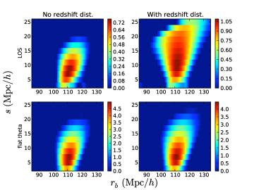
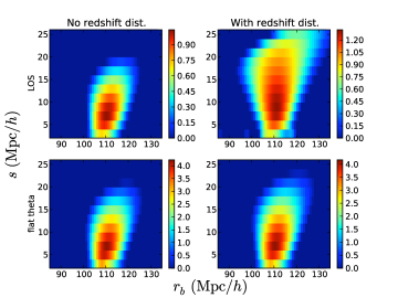
Figs. 4 and 5 show the wavelet S/N from this ensemble of simulations, with and without slicing. Linear redshift distortions are induced along the LOS -axis, and two slicings are taken, along the and axes. The slice thickness used is , which is the physical slice thickness of the SDSS slices at a distance of about 370.
Each 4-plot figure shows the S/N in real and redshift space, and weighting with two different angular weightings in the plane: along the LOS (within of the LOS, ); and with flat weighting in . In no case do we include the weighting typically used in angular averages of for 3D samples. Such a weighting would be inappropriate for the 2D slices that we consider. Also, we do not wish to kill the signal along the LOS.
In all cases, the S/N quoted is that expected from a single simulation box, i.e. it is the mean divided by the standard deviation of the wavelet transform, measured over the 1400 simulation boxes. Note that along the LOS, the S/N is enhanced for the averages of 2D slices. This is even while missing some diagonal modes in the box, since we use only 2 slicing orientations (along axes). Most of the modes very close to the LOS are picked up in at least one of the two orientations, but in the flat weighting, many diagonal modes are missing. This is likely why, with flat weighting, the S/N degrades with the slicings.
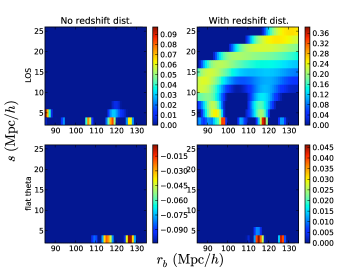
Figs. 6 and 7 show the analogs of the previous two figures, using no-wiggle power spectra. The features detected in the no-wiggle case are generally small in amplitude. However, there is a ridge with S/N reaching from to increasing along the LOS, for the redshift-distorted . This ridge is likely from where the dip at flattens out. This is a region where the second derivative is substantially negative, but where the first derivative is positive (thus it is not, strictly speaking, a peak). There are also peaks at with fairly high significance. These are excluded from the peak-finding below, since they lie along an edge of the searched prior in .

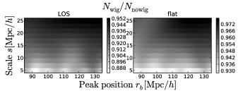
A proper test against the null hypothesis of no BAO feature would use the variance from a no-wiggle power spectrum, but instead, below we estimate variances from the sample itself. Thus it is relevant to ask how the BAO feature affects the standard deviation of the wavelet transform. Fig. 8 shows the ratio of the noise with and without the BAO feature, for both LOS and flat weighting. Typically, the ratio is within 10% of unity, with only very slight fluctuations in .
3.4. Peak-finding Statistics and Systematics in Gaussian fields
In each simulation, we find the maximum of its wavelet transform over a grid , with a grid spacing of . We require that peaks not be along a rectangle-edge in or ; a peak along an edge might indicate that a true peak would be outside the area searched. Thus, the actual possible range for peaks is a bit smaller, . In Bayesian language, this is the range of our flat prior. The error bars that we quote in are marginalized over this flat prior in .
One might worry about covariance as a function of in the S/N plot, and whether it affects our estimate of either the significance, or location, of the bump. Certainly, the wavelet coefficients at nearby are correlated (though less-so than in the raw ). The smoothness of the S/N plots is a sign of this. But this correlation does not affect the interpretation of the S/N: at , it is a good measure of the confidence that a bump exists there, specifically that the Mexican hat wavelet coefficient is positive at that . It does not matter that nearby in and , the S/N is likely quite similar. Covariance in the wavelet coefficient also does not affect the peak location estimate, except that a particular wavelet choice could produce a broader-than-optimal peak in the S/N plot. We have not attempted to optimize or orthogonalize our wavelet, but as we find below, the statistical and systematic errors on the true bump location in Gaussian simulations are still small.
3.4.1 Statistical errors
Figs. 9, 10, 11 and 12 show 2D histograms of peak positions for individual redshift-distorted realizations in the ensembles whose mean S/N plots appear on the right-hand sides of Figs. 4, 5, 6 and 7. The case most relevant to our SDSS measurements is shown in Fig. 10, in which averaged 2D slice correlation functions, drawn from a simulations with BAO features, are analyzed.
In the presence of a BAO feature, the (posterior) distributions of peak ’s after peak-finding are tightened considerably compared to the prior. The set of ’s in the flat prior have a standard deviation of 14, which contracts to 8 when looking along the LOS, and to 2 (we conservatively round up) in the case of flat weighting. In contrast, if there is no BAO feature, the posterior distribution of is hardly narrower than the prior. In the left panel of Fig. 10, there are a couple of curious accumulations of very narrow peaks, along the edge. However, they do not appear to be related to the peaks in the cases with BAO features. True features are somewhat extended in ; we suspect that these narrow features are simply noise.
As recently stated by Cabré & Gaztañaga (2010), the model-comparison question of whether a BAO feature exists in a given sample is quite different than the question of its constraining power. Under the reasonable assumption that the power spectrum underlying the structure in our Universe has a BAO feature, even a low-significance bump gives substantial constraining power. For example, if there happens to be a LOS wavelet S/N peak in a sample, we find that the LOS weighting gives an error bar, even though about half of the mocks possess no LOS peak at all (see Fig. 13).
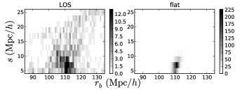
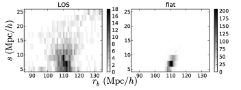
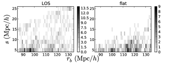
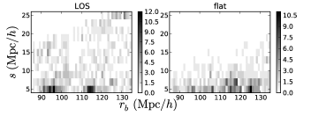
One might also wonder whether error ellipses on the peak and can be inferred directly from the S/N plots. Comparing the S/N plots to the distributions of peaks in Figs. 9, 10, 11 and 12, it seems that there is only a loose relationship. For the two to correspond exactly, the probability of a given having a global peak would have to be simply related to its local S/N value. Given the additional complication of correlations in the S/N plot, it is perhaps not surprising that they are not simply related. One curious difference is that peaks seem more prevalent at small than the mean S/N plots would suggest, especially for flat angular weighting.
3.4.2 Frequency of maximum S/N
The previous section concerned the expectation value of the S/N in the wavelet transform. But if the peak in S/N is broad, the maximum S/N measured in an individual realization will tend to exceed the maximum in the mean, since nearby coefficients may fluctuate independently, and each might produce the observed peak.
Fig. 13 shows the cumulative frequency over 1400 Gaussian simulations of the maximum S/N in various scenarios. For this plot, peaks in were sought in a narrower range of than in the previous sections, more indicative of the peaks actually observed in the SDSS sample. As previously, peaks were excluded if they were along an edge in or ; the actual range of peaks allowed was 100 to 120. The fraction of simulations with a true peak (not on an edge of the prior) can be read off as the fraction with .
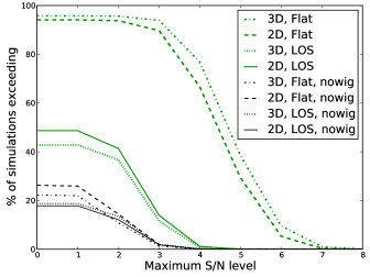
From this figure, we see that if the underlying power spectrum has a BAO feature, using our method it is not uncommon to get a peak up to 3 from a Gaussian sample with the SDSS volume, even along the LOS. Below we estimate the S/N of our bump detection at the peak () to be 2.2 (LOS weighting) and 4.0 (flat weighting). If the underlying power spectrum has a BAO feature, about 40% of the simulations had a LOS peak of S/N , and about 70% had a peak with flat weighting of S/N .
On the other hand, if the underlying power spectrum does not have a BAO feature (i.e. in the null hypothesis of BAO peak detection), it becomes much more uncommon to get such peaks. About 11% of no-wiggle simulations had a LOS peak of S/N , and about 0.2% of no-wiggle simulations had a peak with flat weighting of S/N .
3.4.3 Systematic errors
The Mexican-hat wavelet transform is a natural measure of the second derivative at position , if the function it is applied to is smoothed over a scale . In fact, arguably a peak in the Mexican-hat wavelet coefficient would be a good definition of the peak position itself, if at an appropriate scale. An alternative definition is the actual local maximum of the peak in the linear correlation function. However, this definition can cause a bias, if the peak is on top of a slope, as mildly occurs in the case of a CDM correlation function. Fig. 14 shows computed using a camb power spectrum, along with the difference between that and a no-wiggle . Both are measured from density fields with exactly the Fourier amplitudes prescribed by their linear power spectra. The peaks of , and of the difference, are at 109.5 and 110.3, a shift of almost 1.
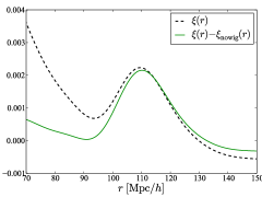
The means in the peak distributions shown in Figs. 4 and 5 are within of both peaks shown in Fig. 14, if the peak is defined as the actual local maximum of the peak in , the wavelet estimator tends to overestimate the peak location by about .
Again, the small systematic errors found here come from purely Gaussian simulations, without nonlinearities or galaxy bias, which could generate their own systematic errors, perhaps of order the statistical error bars in our sample.
4. Measurements from the Millennium simulation
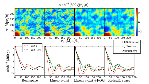
We compare our results from the observations with simulations of large-scale structure formation. We used Millennium-simulation (MS) galaxies to investigate realistic redshift distortions of galaxy samples. However, its box size (), smaller than the size of our sample, and the fact that we only have a single realization, make it insufficient to derive strong conclusions about the detailed statistics of BAO measurements. So, we also employed Gaussian simulations to get a better idea of the correlations involved, keeping in mind that non-linearities would likely degrade significances and constraints we measure.
Figure 15 shows various correlation functions of galaxies from the MS, measured on a grid. The galaxies used were brighter than an -magnitude of (absolute) as modeled by De Lucia & Blaizot (2007), giving a mean density of 0.02 .
The curves shown are averages of slice correlation functions over all possible orientations, axes, and slice locations. For the real-space ’s, the grid was split into 64 slices of thickness along all three Cartesian axes, giving ’s to average together. In the middle two columns, linear redshift-space distortions were generated analytically, using and in the Kaiser formula
| (36) |
where . In the right column, redshift-space distortions were generated using the actual MS galaxy velocities, not an approximate model. In each case, the result is an average over all possible permutations among the three axes of the LOS and the two axes along which the slices were cut.
Generally, linear-theory redshift-space distortions in 2D slices do appear to sharpen the baryon bump in relative to real space. Indeed, as we find below with Gaussian simulations, linear redshift-space distortions seem not only to sharpen the peak, but to increase its robustness too, at least when it is analyzed using wavelets. At some level, one expects fingers of God (FoG) tend to degrade all features in , even away from the LOS. Interestingly, though, at least in the MS, the 1D curves do not change much between the two bottom-middle plots, suggesting that the fogginess effected by FoG may be minor.
We applied the wavelet analysis to the redshift-space MS simulations, as well. Fig. 16 shows the mean S/N from these samples. With flat weighting in angle, there is a shift relative to the Gaussian peak location. It would be tempting to use this as an estimate of the systematic error from using a simulation with full non-linearities and galaxy formation, but it could very well be a statistical fluctuation instead.
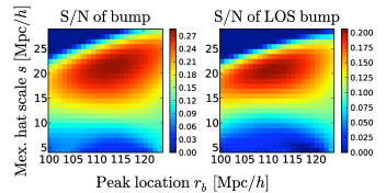

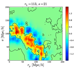
Fig. 17 shows measurements of for MS galaxies, and in linear theory. In these figures, the values of and are those at the peaks in the signal-to-noise ratio of the wavelet transform .
5. Measurements from the SDSS
5.1. The Sample
We analyzed the SDSS DR7 (Abazajian et al., 2009) main-galaxy sample (MGS Strauss et al., 2002). These are all galaxies observed by SDSS that have an R-band Petrosian magnitude R. Importantly for our analysis, their redshifts have been measured spectroscopically. We selected galaxies designated as sciencePrimary, from the Northern cap of SDSS, in stripes 9 through 37, with a redshift confidence 0.9, and redshift error 0.1. We also cut galaxies from the tails of the selection function, including only galaxies with distance . This gave us a total of 527,781 galaxies to begin with. Furthermore, there were several regions with ’holes’ and small, incompletely sampled regions in stripes 13, 29, 35 and 36. We removed all objects in these incomplete areas. This left us with a total of 527,362 objects.
We have computed comoving radial distances for each object, expressed in , using built-in functions in the SDSS SkyServer database (Taghizadeh-Popp, 2010), with , and . The angular coordinates were converted to Cartesian, and rotated to a coordinate system, whose z-axis was along the SDSS North Pole, at ra=185, dec=32.5. Each of the normal vectors were then multiplied with the computed radial distance to give us a 3D location.
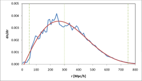
We computed a smooth polynomial fit to the redshift distribution, , using a 6th order polynomial in . The curve is shown in Fig. 18. We used the angular selection mask, defined by boundaries of the selected stripes and the censored ’holes’ and this analytic radial distribution to generate 17M random galaxies with the correct geometric properties. Each random galaxy had an additional random number precomputed, making it easy to select decimated subsets for further analyses.
These two data sets were then stored in two database tables. We created a simple function that was able to take an arbitrary rotation of the samples around the -axis. We stepped the rotation angle in 15 increments, from to , for a total of 12 angular orientations. For each orientation we extract thick slices, resembling the original SDSS stripes, except for the rotation. We eliminated slices which contained only a small fraction of the data, located at the edges of the survey, i.e. slices of width . Slices that were wider than were split in half across, so that no slice exceeded the width of . This gave us 661 slices.
5.2. Computing the Correlations
We used the Landy & Szalay (1993) estimator to estimate the correlations, for its optimal behavior (Kerscher et al., 2000):
| (37) |
where , and are numbers of pairs of random and actual (data) galaxies, in length bins of .
Measuring the distances among all random and data galaxies is inherently an problem. The current state-of-the-art solution by Moore et al. (2001) involves binary trees built on the datasets, and uses a dual-tree traversal algorithm. The idea is to speed up the procedure by checking distance constraints on pairs of tree-nodes that represent 3-D boxes. If all pairs of points coming from the cells fit in a single bin, one can increment the counts and stop going deeper on that branch. For low-resolution 1-D statistics, such as the angular correlation functions measured in a dozen logarithmic bins, the above procedure can indeed increase the performance tremendously especially when one is interested in small-scale clustering and able to discard early all pairs of large separations. Our problem is more difficult: here we measure the the two-dimensional redshift-space - correlation function out to the largest scales at high resolution in 000 bins of spacing Mpc. (To eliminate null pixels in the region of interest, however, we ended up degrading the resolution to 2 Mpc.) The dual-tree code slows down in this high-bin limit and becomes essentially as expensive as the brute-force naive method.
Our solution is to implement the counting on modern graphics processing units (GPUs) that offer hundreds of cores and run tens of thousands of threads simultaneously on commercial video cards. We use NVIDIA’s Compute Unified Device Architecture (CUDA) to implement the parallel correlation function code in the C++ programming language and integrate it with SQL Server where the data reside. Using SQL wrapper routines, we run the analysis directly on GTX 295 GPUs without temporary intermediate file storage. The performance is hundreds of times faster on this parallel architecture when compared to todays CPUs, which is not too surprising for the large number of algorithm logic units (480 ALUs) on these cards. The results from the GPUs are returned in database tables, stored and further analyzed in SQL to compute the final correlation functions.
The 2D correlation function was computed for each slice, with a 2 resolution, out to 570 in each direction. A total of 400 trillion galaxy pairs were computed, including both real and random points.
5.3. Results from the SDSS
Fig. 19 shows from two samples: first, the full sample, including all galaxies from , and a high-redshift sample, . Along the LOS, the full sample has two prominent peaks: one at about , and a second at about . The first could be associated with a BAO feature, but the second could not, given plausible priors on the BAO scale from previous measurements (e.g. Eisenstein et al., 2005).
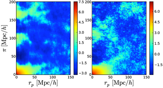
We analyzed the higher-redshift sample because the measurement gives perhaps undue weight to the densely sampled structures at low redshift, such as the Sloan Great Wall. Including the Sloan Great Wall, which is at a distance of about 220 (Gott et al., 2005), is known to change clustering statistics substantially (e.g. Nichol et al., 2006), producing an upward fluctuation in Fig. 18 of 20%.
A better solution might be to reduce the additional cosmic variance from such a structure by down-weighting it, e.g. with a Gaussianizing density mapping (Neyrinck et al., 2009), but for the present paper we simply cut the near part of the sample, within 300, and apply an additional weighting to each galaxy. By volume, this high- sample is only 6% smaller than the the full one, although it only contains about half the galaxies, 261,737. The effective volume including shot noise (Tegmark, 1997)
| (38) |
for the full sample is . For the high- sample, , a 9% difference. Here we use (from the linear power spectrum used in the Gaussian simulations, at about the BAO scale in wavenumber), assuming a -steradian survey.
The optimum (minimum variance) spatial weighting for galaxies at radial distance , on the clustering scale is given by (Kaiser, 1986)
| (39) |
For the SDSS main-galaxy sample, . Using the selection function of the galaxies we can compute the weight corresponding to the 110 scale. We then fit a third-order polynomial to the log of the weight function, and use this analytic expression in the further analysis.
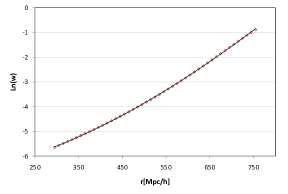
Fig. 20 shows the spatial weighting function. Due to the large change in the weight function from the near to far edge, we experimented with different choices for the weighting, applied to each galaxy: (a) uniform weighting, (b) , (c) . We found that (c) results in a substantially increased shot noise, since there is too much weight added to the small number of objects at the far edge of the volume, while there is very little difference between (a) and (b). As a result, we adopt (b), the square-root-weighted high- sample, as our fiducial one for analysis. Indeed, cutting galaxies closer than does entirely remove the feature.

Figure 21 shows flat angle-averaged, and LOS, correlation functions for MS and Gaussian samples, and for the high- SDSS sample. No galaxy-bias factor was applied to the Gaussian curves.
In each case, is measured among 2D slices, and then averaged together. The error bars are rather different in size; this is because of the different sample volumes. Also, as usual in discussions of the correlation function, we should note that the error bars are somewhat correlated.
The Gaussian error bars are the simulation-to-simulation standard deviations of , measured in 2D slices (using only one slicing orientation) and then averaged together. In the MS and SDSS cases, the error bars are estimated from within the sample of slice correlation functions, requiring an estimate of the number of degrees of freedom (DOF) among the correlated slices. The square root of this DOF is the factor by which we divide the slice-by-slice dispersion to get the plotted error bars.
In the MS case, the flat-angular-weighting DOF is the number of slices (128 = 2 axes 64 slices per axis) divided by 1.2, the same factor used below in Section 5.4.1 from the Gaussian simulations to account for the additional cosmic variance from going from ensembles of slices to ensembles of simulations. The DOF in the LOS case gets divided by an additional, conservative factor of two because many LOS pairs of galaxies are present in slices along both slicing directions. We were particularly careful for the SDSS sample in estimating the reduction in DOF from correlated slicing orientations; see Sect. 5.4 below for details.
The flat-angular-weighting ’s in the SDSS and MS samples are strikingly similar in shape. In fact, we do not necessarily expect the samples to match, since the galaxy properties or number densities do not match between the MS and SDSS samples. We consider the high degree of agreement to be largely by chance.
One feature that seems quite solid, though, is a LOS trough at (see also Fig. 26, below), that is much deeper than the Gaussian simulations. Multiplying the Gaussian curve by some linear bias factor could perhaps make these troughs line up better, but this would cause disagreement at larger , and would require quite a large bias factor, which we do not expect for this relatively low-luminosity sample. The depth of the trough is a sign that non-linear infall and/or galaxy bias clear out this region along the LOS much more dramatically than in linear theory. We speculate that in the SDSS case, one reason for the strong peak along the LOS is a pile-up of these cleared-out galaxies.
5.4. Effective degrees of freedom
While our slicing strategy enables an estimate of error bars and signal significance, this estimate is rather complicated, since slices overlap, and even when they do not, nearby slices are likely correlated with each other. If all slices were statistically independent, the degrees of freedom (DOF) would be the number of slices, 661. We investigate two factors by which this number must be reduced: first, a factor coming from slice correlations and cosmic variance; second, a factor from overlap due to the 12 different angular slicings.
5.4.1 Correlated slices and cosmic variance
We typically expect an overestimate in the significance level of a detection when estimating it from within the sample. We investigate this effect on Gaussian simulations to which linear redshift distortions have been applied.
As in Section 3.3, we sliced Gaussian simulations (box size 768, cell size ) into 16 slices. Here, we take just one slicing per simulation. From each simulation, we estimate (S/N)slices of the wavelet coefficient at each by measuring the mean and standard deviation among slices within the simulation. In this case, we multiply the S/N by , the DOF of the single slicing in the approximation that all slices are independent. We also measure (S/N)slicings more properly, measuring the mean and standard deviation of averages of slicings of different simulations. The latter estimate, which includes the effects of slice-to-slice correlation and cosmic variance, is the same as those performed in Section 3.3, except that here, one (instead of two) slicing orientation is used.
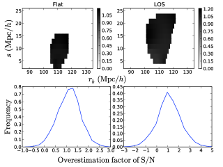
Fig. 22 shows the means and distributions of the ratio of (S/N)slices, which is different for each simulation, to (S/N)slicings. We expect it to exceed one on average, since estimating the significance among slices should give an overestimate. In the top row, the dark regions are within the “peak region,” defined as having a (S/N)slicings of at least half the maximum (S/N)slicings. We focused on this peak region to avoid dividing by small numbers when taking the ratio. The bottom row shows histograms of this ratio over all simulations, and over all in the peak region. Results are shown for both ’flat’ and LOS angular weighting.
Although we have used simulations with about the same volume as the SDSS sample, again they are purely Gaussian simulations, with linear redshift distortions. The slice-to-slice variance in the wavelet coefficient is surely underestimated using them. However, in Gaussian simulations, the simulation-to-simulation variance is likely underestimated as well, so we expect their ratio (which is what actually enters our SDSS analysis) not to be underestimated as severely as the slice-to-slice variance in the wavelet coefficient.
The mean of this ratio of standard deviations in the peak region is only a bit over 1; the mean in both LOS and flat weightings is 1.1. Thus we adopt as the DOF reduction factor from going from slice-to-slice variance to simulation-to-simulation variance. We should note that there is a large dispersion in this factor, which simply means that a given simulation can have a much larger or smaller signal than the mean would give.
5.4.2 Correlated slicing orientations
The factor by which we would overestimate the DOF by assuming all slicings to be independent is , where is the number of slicings, and is the number of slicings including degeneracy. Roughly, , the mean number of slices occupied by a pair of galaxies. We estimate in two ways: first, by counting galaxy pairs that go into the 2D and 3D correlation functions. Second, we relate the problem to that of Buffon’s needle (Buffon, 1777).
To estimate in a brute-force fashion, we add up the raw number of galaxy pairs (), counted in all 661 2D slices, as a function of in the plane. We also measure the pairs in 3D, and compare them. Using a range in of 100-120, we count the pairs in 1-wide bins. Fig. 23 shows the ratio of the 2D to 3D pairs. In the limit of small sky separation, we expect all pairs to enter 12 slices. The reason that the plotted ratio exceeds 12 at small separation is because of the slices’ 2D projection, important for (the slice width): a pair’s 3D gets projected onto the plane of the slice, resulting in a smaller 2D . Also note that at large , the fraction dips below 1. This means that the 12 slicings were not enough to catch all pairs at large angles.
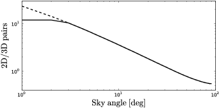
To estimate for the two weightings, we average the plotted ratio from 0 to 6 (LOS), and from 0 to 90 (flat). Since pairs cannot inhabit over 12 slices, for this average we truncate the curve at 12. Averaging this truncated curve gives (LOS) and (flat).
Another, analytical way of estimating the the number of slices on average that a pair of galaxies inhabits is related to the problem of Buffon’s needle, which can be stated as follows: Let denote the probability that a needle of length , dropped randomly on a piece of paper with parallel lines separated by a distance , will cross at least one line. Buffon found that
| (40) |
The expression is more complicated if , but we do not use that case here.
Associating galaxy pairs with “needles,” and slice edges with the parallel lines on the paper, a galaxy pair will inhabit a slice if it does not cross any lines. Imagining a slice orientation as a random rotation and translation of the lined paper, the fraction of slice orientations for which a galaxy pair (of separation on the sky) appears in a slice (of angular thickness ) will be . With 12 orientations, the average number of slices occupied per galaxy will be .
If the angle in the plot were the angle on the sky, we would simply average over a range of to get the average LOS galaxy-pair-slice occupancy. We work in coordinates though, so we estimate a maximum around the BAO scale along the LOS to be about 1/3.5 of the maximum angle in . This 1/3.5 factor is a typical ratio of their LOS separation () to the LOS distance to the observer (). Averaging over angles from to gives 9.4 slices, in accord with the previous estimate based on pair counts.
To illustrate the degree of independence of among the 12 slice orientations, we plot for each orientation, and also its mean. Fig. 25 shows this for LOS and flat weightings. As expected from the arguments in this Section, there is much more variance with flat weighting than LOS, since the galaxy pairs along the LOS occupy slices of many slice orientations.
6. Wavelet analysis of the SDSS Results
We apply the same wavelet-based peak finder described in the previous sections to the high-redshift SDSS results. Fig. 24 shows the results. The top panels shows the S/N from this sample, with LOS and flat angular weighting, over the same range (i.e. Bayesian prior) in () as in the Gaussian simulations. Here the raw inter-slice S/N is divided by the effective number of degrees of freedom (DOF), discussed in Section 5.4. If the slices were independent,the DOF would simply be the number of slices, 661. But this needs to be reduced by a factor from slice correlation and cosmic variance (which we estimate to be 1.2), and a factor from physical slice overlaps from the multiple slicing orientations (which we estimate to be 9.2 for LOS weighting, and 1.7 for flat weighting). With this correction, we estimate the peak S/N of the LOS peak to be significant at the 2.2- level, and the peak with flat angular weighting at the 4.0- level. As in the previous result plots, we weight each slice by its width.
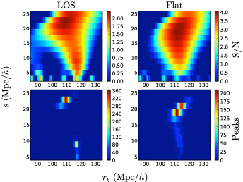
The bottom panels show 2D histograms of peak locations from 3000 bootstrap-resamplings of 661 slices (with replacement) from the 661 slices. Because we use the same number of slices in the bootstrap samples as in the measurement, this gives an estimate of the actual uncertainty in the peak positions, estimated from within the sample itself.
The peak locations, with error bars thus estimated from within the sample, are (LOS), and . These error bars consider some cosmic variance, but only that found within the sample. To this, we add in quadrature the error bars from cosmic variance outside the sample, estimated from the Gaussian simulations (which give error bars of in LOS, and with flat weighting). This gives estimates of (LOS) and (flat). These do not include systematic error bars, which above we estimated to be about for the Gaussian simulations, but would likely be larger for fully non-linear simulations.
The S/N peaks in both the MS and SDSS samples are at substantially higher than in the Gaussian simulations. One possible cause for this is the broadening in the BAO feature that Lagrangian displacements of order from large-scale tidal motions produce (e.g. Eisenstein et al., 2007). Also, fingers of God likely broaden the peak in the LOS direction.
Of course, our Gaussian simulations we use here are idealized, missing several complications that are mild but perhaps not entirely negligible on BAO scales: non-linearities in matter clustering; shot noise; effects from the non-cubic, non-periodic survey shape; bias between the galaxy and matter fields; non-linear redshift distortions, especially fingers of God; and perhaps large non-Gaussian (co)variance (Rimes & Hamilton, 2005), which however seems a bit milder for redshift-space galaxies than for real-space matter (Neyrinck et al., 2010).
To get an iron-clad estimate of the significance, we need high-resolution Gpc-scale simulations, that would both encompass a representative volume, and possess full non-linearities. This will be part of a follow-up analysis, where we will build a few hundred rather high-resolution simulations, analyzed using realistic, SDSS-like survey geometries.
In the mean time, because these constraints will likely enlarge in the face of non-linearities, we conservatively adopt the looser constraint on the BAO peak position, that comes from the LOS weighting, rounding up the error bar to . This error bar is likely larger than any additional systematic errors from non-linearities. Also, it would accommodate the peak in the full (including the Sloan Great Wall) sample, which is at 97.
While 4.0 is a measure of the S/N of a bump in the SDSS sample at the particular peak () in the S/N plot, the percentages given at the end of Section 3.4.2 give another measure of the significance of our peak detection, that is immune to a posteriori bias issues. 0.2% of no-wiggle simulations have any bump of S/N that could plausibly be associated with the BAO feature (i.e. that is between 100 and 120. This implies a 99.8% chance that a bump such as we see (i.e. anywhere in the vicinity of the expected BAO location) is truly a BAO feature.
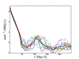
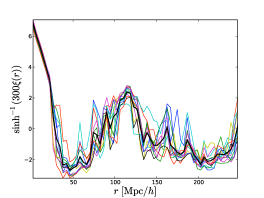
In another test, that does not depend at all on Gaussian simulations, we use the variances among the 12 slicings of the wavelet transforms of correlation functions, averaged over all slices within the slicing. Fig. 25 shows these correlation functions, along with their mean. As expected, the LOS dispersion is smaller than with flat weighting, since the LOS measurements are highly correlated from slicing to slicing. In contrast, the predicted simulation-to-simulation variance in the LOS is greater than with flat weighting; this is why our stated S/N level is lower with LOS than with flat weighting.
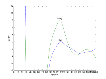
Fig. 26 shows the wavelet transform’s S/N as a function of , holding the wavelet scale fixed at , using the raw, slicing-to-slicing dispersion for the noise N. This gives a LOS peak S/N of 7.9, and a flat-weighting S/N of 1.9. This is without reducing the noise (by the square root of the effective DOF) because we are averaging the results of different slicings together. The effective DOF is the effective number of independent slicings; These are (LOS), and (flat), bringing the estimated S/N to 9.0 (LOS) and 5.2 (flat). The LOS significance, in particular, seems ridiculously large, but we must remember that it is based on only 1.3 effective measurements; including the error bar (fractionally, ), the S/N is . The slicing-to-slicing estimate of the flat S/N is more meaningful, . We should note that this estimate does neglect slicing-to-slicing correlation that goes beyond actual overlaps of galaxy pairs, but we expect this additional correlation to be small.
Fig. 26 also shows the tremendous significance of the trough at . We speculate that this trough is cleared out to a greater degree in the presence of a BAO peak, and this is an interesting issue for further study.
7. Conclusion
In this paper we have shown how redshift space distortions can amplify and modify features in the galaxy correlation function. In linear theory, the BAO feature sharpens as the angle approaches the line of sight. While we expect nonlinear effects such as fingers of God to broaden the BAO feature along the line of sight (LOS), they do not seem to dampen it substantially.
We see a compelling LOS “bump” in the SDSS DR7 MGS correlation function, measured in 2D slices of varying pitch angle that cover the sample. We analyze the bump using a Mexican-hat wavelet transform, which has a peak in signal-to-noise ratio S/N at , marginalized over the scale of the wavelet. We assess the significance of the bump by looking at variances of slice correlation functions within the sample, which presents difficulties because of slice-to-slice correlations. Nevertheless, at the particular location and wavelet scale of the peak in wavelet S/N, we tentatively assess the significance of this peak at 4 if the correlation function is averaged in a flat angular weighting, and at 2.2 if it is averaged only within of the line of sight.
These significance estimates employ Gaussian simulations, and thus are likely a bit optimistic. However, this optimism is more modest than it might at first seem; we only use the Gaussian simulations to extrapolate the significance estimate measured from slices within the sample to the proper, sample-to-sample significance estimate. We make another estimate that does not use simulations at all. From just the variance of the wavelet transform among angular slicing orientations, we estimate that the S/N (LOS) and S/N (flat weighting).
Taking into account a posteriori bias, we also ask how common a bump of the measured significance is in Gaussian no-wiggle simulations, not just at the peak of the wavelet S/N, but anywhere in the vicinity of the BAO feature (within 10 of 110). Evaluating the wavelet using flat angular weighting, we find that such a bump is only present in 0.2% of no-wiggle simulations.
It is curious that the LOS BAO feature seems to be stronger than apparently expected from simulations, in both the Sloan LRG (Gaztañaga et al., 2009) and main-galaxy samples. Its presence in both, rather independent, samples suggests that this is not a fluke.
We propose that the weighting that is commonly used, while sensibly motivated since it follows the distribution of galaxy pairs in a 3D sample, is likely suboptimal in constraining power, since it greatly suppresses any LOS signal. An example of an alternative weighting that is less hostile to the LOS is the flat weighting we employ, which is natural for the 2D slicing strategy we use.
While our current analysis makes the case that the features we see are rather statistically significant, a conclusive determination awaits a planned study employing more-realistic simulations, that include nonlinearities, galaxy bias, survey-shape effects, etc. This study will not only address our present result specifically, but we hope will provide a definitive answer the question of how BAO constraining power varies with angle from the LOS.
Our claimed rather high significance level may be surprising in light of recent analyses casting doubt on the reality of BAO detections even in the larger, SDSS LRG sample (Kazin et al., 2010; Cabré & Gaztañaga, 2010). In these analyses, if a correlation function is better-fit by a “no-wiggle” model, there is deemed not to be a bump. Although we do not quantitatively compare the methods, our peak detector is likely more tolerant of modest bumps. For us, essentially there exists a bump at a certain wavelet scale and location if the correlation function has a positive wavelet coefficient there, i.e. that the second derivative of the correlation function, smoothed over the wavelet scale, is negative.
Even if we have overestimated the significance of our detection, an important point is that it still may be used for cosmological constraints. As Cabré & Gaztañaga (2010) emphasize, the hypothesis test that a BAO feature exists in a given sample is a separate statistical question from the degree of its cosmology-constraining power. There is essentially no doubt that the power spectrum underlying the structure in our Universe had a BAO feature at the epoch when the cosmic microwave background was emitted (e.g. Larson et al., 2010), and if it is not present at the present epoch, that would be a big cosmological puzzle.
Under the assumption that the power spectrum underlying the structure in our Universe has a BAO feature, we find that the appearance of even a low-significance bump gives some constraining power over the BAO feature’s location. For example, in a Gaussian sample with the volume of ours, if a clear bump exists in a sample (which happens about half the time), the bump gives an error bar in the BAO peak location of .
References
- Abazajian et al. (2009) Abazajian, K. N. et al. 2009, ApJS, 182, 543, 0812.0649
- Bond & Efstathiou (1984) Bond, J. R., & Efstathiou, G. 1984, ApJ, 285, L45
- Bond & Efstathiou (1987) ——. 1987, MNRAS, 226, 655
- Broadhurst et al. (1990) Broadhurst, T. J., Ellis, R. S., Koo, D. C., & Szalay, A. S. 1990, Nature, 343, 726
- Buffon (1777) Buffon, G. 1777, Histoire naturelle, générale et particulière, Supplément, 4, 100
- Cabré & Gaztañaga (2010) Cabré, A., & Gaztañaga, E. 2010, ArXiv e-prints, 1011.2729
- Cole et al. (2005) Cole, S. et al. 2005, MNRAS, 362, 505, arXiv:astro-ph/0501174
- Colless et al. (2001) Colless, M. et al. 2001, MNRAS, 328, 1039, arXiv:astro-ph/0106498
- de Bernardis et al. (2000) de Bernardis, P. et al. 2000, Nature, 404, 955, arXiv:astro-ph/0004404
- de Lapparent et al. (1988) de Lapparent, V., Geller, M. J., & Huchra, J. P. 1988, ApJ, 332, 44
- De Lucia & Blaizot (2007) De Lucia, G., & Blaizot, J. 2007, MNRAS, 375, 2, arXiv:astro-ph/0606519
- Eisenstein & Hu (1998) Eisenstein, D. J., & Hu, W. 1998, ApJ, 496, 605, arXiv:astro-ph/9709112
- Eisenstein et al. (2007) Eisenstein, D. J., Seo, H., & White, M. 2007, ApJ, 664, 660, arXiv:astro-ph/0604361
- Eisenstein et al. (2005) Eisenstein, D. J. et al. 2005, ApJ, 633, 560, arXiv:astro-ph/0501171
- Gaztañaga et al. (2009) Gaztañaga, E., Cabré, A., & Hui, L. 2009, MNRAS, 399, 1663, 0807.3551
- Gott et al. (2005) Gott, III, J. R., Jurić, M., Schlegel, D., Hoyle, F., Vogeley, M., Tegmark, M., Bahcall, N., & Brinkmann, J. 2005, ApJ, 624, 463, arXiv:astro-ph/0310571
- Hamilton (1992) Hamilton, A. J. S. 1992, ApJ, 385, L5
- Hamilton (2009) Hamilton, A. J. S. 2009, in Lecture Notes in Physics, Berlin Springer Verlag, Vol. 665, Data Analysis in Cosmology, ed. V. J. Martínez, E. Saar, E. Martínez-González, & M.-J. Pons-Bordería, 415–431, arXiv:astro-ph/0503603
- Hamilton & Culhane (1996) Hamilton, A. J. S., & Culhane, M. 1996, MNRAS, 278, 73, arXiv:astro-ph/9507021
- Hanany et al. (2000) Hanany, S. et al. 2000, ApJ, 545, L5, arXiv:astro-ph/0005123
- Heavens & Taylor (1995) Heavens, A. F., & Taylor, A. N. 1995, MNRAS, 275, 483, arXiv:astro-ph/9409027
- Holtzman (1989) Holtzman, J. A. 1989, ApJS, 71, 1
- Kaiser (1986) Kaiser, N. 1986, MNRAS, 219, 785
- Kaiser (1987) ——. 1987, MNRAS, 227, 1
- Kaiser & Peacock (1991) Kaiser, N., & Peacock, J. A. 1991, ApJ, 379, 482
- Kazin et al. (2010) Kazin, E. A., Blanton, M. R., Scoccimarro, R., McBride, C. K., & Berlind, A. A. 2010, ApJ, 719, 1032, 1004.2244
- Kerscher et al. (2000) Kerscher, M., Szapudi, I., & Szalay, A. S. 2000, ApJ, 535, L13, arXiv:astro-ph/9912088
- Landy et al. (1996) Landy, S. D., Shectman, S. A., Lin, H., Kirshner, R. P., Oemler, A. A., & Tucker, D. 1996, ApJ, 456, L1+, arXiv:astro-ph/9510146
- Landy & Szalay (1993) Landy, S. D., & Szalay, A. S. 1993, ApJ, 412, 64
- Larson et al. (2010) Larson, D. et al. 2010, ArXiv e-prints, 1001.4635
- Lewis et al. (2000) Lewis, A., Challinor, A., & Lasenby, A. 2000, ApJ, 538, 473, arXiv:astro-ph/9911177
- Miralda-Escude (2009) Miralda-Escude, J. 2009, ArXiv e-prints, 0901.1219
- Moore et al. (2001) Moore, A. W. et al. 2001, in Mining the Sky, ed. A. J. Banday, S. Zaroubi, & M. Bartelmann, 71, arXiv:astro-ph/0012333
- Neyrinck et al. (2006) Neyrinck, M. C., Szapudi, I., & Rimes, C. D. 2006, MNRAS, 370, L66, arXiv:astro-ph/0604282
- Neyrinck et al. (2009) Neyrinck, M. C., Szapudi, I., & Szalay, A. S. 2009, ApJ, 698, L90, 0903.4693
- Neyrinck et al. (2010) ——. 2010, ApJ, submitted, 1009.5680
- Nichol et al. (2006) Nichol, R. C. et al. 2006, MNRAS, 368, 1507, arXiv:astro-ph/0602548
- Padmanabhan et al. (2007) Padmanabhan, N. et al. 2007, MNRAS, 378, 852, arXiv:astro-ph/0605302
- Pápai & Szapudi (2008) Pápai, P., & Szapudi, I. 2008, MNRAS, 389, 292, 0802.2940
- Peebles & Yu (1970) Peebles, P. J. E., & Yu, J. T. 1970, ApJ, 162, 815
- Pen et al. (2003) Pen, U., Lu, T., van Waerbeke, L., & Mellier, Y. 2003, MNRAS, 346, 994, arXiv:astro-ph/0304512
- Percival et al. (2007) Percival, W. J., Cole, S., Eisenstein, D. J., Nichol, R. C., Peacock, J. A., Pope, A. C., & Szalay, A. S. 2007, MNRAS, 381, 1053, 0705.3323
- Percival et al. (2010) Percival, W. J. et al. 2010, MNRAS, 401, 2148, 0907.1660
- Rimes & Hamilton (2005) Rimes, C. D., & Hamilton, A. J. S. 2005, MNRAS, 360, L82, arXiv:astro-ph/0502081
- Scoccimarro (2004) Scoccimarro, R. 2004, Phys. Rev. D, 70, 083007, arXiv:astro-ph/0407214
- Silk (1968) Silk, J. 1968, ApJ, 151, 459
- Springel et al. (2005) Springel, V. et al. 2005, Nature, 435, 629, arXiv:astro-ph/0504097
- Strauss et al. (2002) Strauss, M. A. et al. 2002, AJ, 124, 1810, arXiv:astro-ph/0206225
- Sunyaev & Zeldovich (1970) Sunyaev, R. A., & Zeldovich, Y. B. 1970, Ap&SS, 9, 368
- Szalay et al. (1998) Szalay, A. S., Matsubara, T., & Landy, S. D. 1998, ApJ, 498, L1+, arXiv:astro-ph/9712007
- Szapudi (2004) Szapudi, I. 2004, ApJ, 614, 51, arXiv:astro-ph/0404477
- Taghizadeh-Popp (2010) Taghizadeh-Popp, M. 2010, PASP, 122, 976
- Tegmark (1997) Tegmark, M. 1997, Physical Review Letters, 79, 3806, arXiv:astro-ph/9706198
- Tegmark et al. (1998) Tegmark, M., Hamilton, A. J. S., Strauss, M. A., Vogeley, M. S., & Szalay, A. S. 1998, ApJ, 499, 555, arXiv:astro-ph/9708020
- Weiner et al. (2005) Weiner, B. J. et al. 2005, ApJ, 620, 595, arXiv:astro-ph/0411128
- Xu et al. (2010) Xu, X. et al. 2010, ApJ, 718, 1224, 1001.2324