Breakdown of Self-Similarity at the Crests of Large-Amplitude Standing Water Waves

Abstract

We study the limiting behavior of large-amplitude standing waves on deep water using high-resolution numerical simulations in double and quadruple precision. While periodic traveling waves approach Stokes’s sharply crested extreme wave in an asymptotically self-similar manner, we find that standing waves behave differently. Instead of sharpening to a corner or cusp as previously conjectured, the crest tip develops a variety of oscillatory structures. This causes the bifurcation curve that parametrizes these waves to fragment into disjoint branches corresponding to the different oscillation patterns that occur. In many cases, a vertical jet of fluid pushes these structures upward, leading to wave profiles commonly seen in wave tank experiments. Thus, we observe a rich array of dynamic behavior at small length scales in a regime previously thought to be self-similar.

Singularities in fluid mechanics are generally expected to be asymptotically self-similar Eggers and Fontelos (2009). These can be dynamic singularities, such as bubble pinch-off Turitsyn et al. (2009) or wave breaking Bridges (2009), or parametric singularities, where a family of smooth solutions terminates at a singular solution. A famous example of the latter type was posed by Stokes in 1880, who used an asymptotic expansion of the stream function to argue that the periodic traveling water wave of greatest height should have an interior crest angle of $120^{\circ}$. This crest angle has been confirmed in numerous computational studies Gandzha and Lukomsky (2007) as well as theoretically Amick et al. (1982). The asymptotic behavior of the almost highest traveling wave was analyzed by Longuet-Higgins and Fox Longuet-Higgins and Fox (1977, 1978).

Because genuine dynamics are involved, existing numerical methods have been unable to maintain the accuracy needed to fully explore the limiting behavior of large-amplitude standing waves. As a result, Penney and Price’s conjecture Penney and Price (1952) that a limiting standing wave exists and develops $90^{\circ}$ interior crest angles each time the fluid comes to rest has remained open since 1952. Such a singularity would be both dynamic and parametric. The standing waves in question are spatially periodic and have zero impulse (horizontal momentum), maintaining even symmetry for all time. They are also temporally periodic, alternately passing through two zero-velocity rest states of maximal potential energy.

Small-amplitude standing waves of this type were proved to exist by Iooss, Plotnikov, and Toland Iooss et al. (2005). Larger-amplitude waves were computed by Mercer and Roberts Mercer and Roberts (1992), who discovered that the wave steepness (half the crest-to-trough height) does not increase monotonically over the entire one-parameter family of standing waves. They proposed using (downward) crest acceleration, $A_{c}$, as a continuation parameter instead. We reproduce (and extend) their plot of wave steepness versus crest acceleration in Fig. 1. Since pressure increases with depth near the free surface Wu (1997), Euler’s equations imply that $A_{c}$ cannot exceed $g$, the acceleration of gravity.

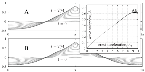
Figure 1: Bifurcation diagram and selected standing waves, plotted at equal time slices over a quarter period. The wavelength is taken to be $2\pi$, and $g=1$. The crest tip sharpens as $A_{c}$ increases over the range $0\leq A_{c}\leq 0.985$, where previous numerical studies are reliable. In particular, the curvature at the crest is visibly higher for solution B than for A.

Taylor Taylor (1953) performed wave tank experiments and confirmed that large-amplitude standing waves do form reasonably sharp crests close to 90 degrees. A further increase in amplitude caused the waves to splash and become unstable in the transverse direction. Grant Grant (1973) and Okamura Okamura (1998) have written theoretical papers to support the $90^{\circ}$ conjecture. Okamura also performed numerical experiments Okamura (2003, 2010) to back this claim. Extrapolating from numerical solutions, Mercer and Roberts Mercer and Roberts (1992) speculated that the limiting crest angle might be as sharp as $60^{\circ}$. Schultz et. al. Schultz et al. (1998) also predicted a limiting wave profile with a crest angle smaller than $90^{\circ}$ and offered the possibility that a cusp may form instead of a corner.

Our objective is to challenge the assumption that standing waves behave as traveling waves in their approach of an “extreme” limiting wave. If there is no limiting wave profile, then a local analysis suggesting a geometric singularity (corner or cusp) is inapplicable.

The equations of motion for a two-dimensional irrotational ideal fluid of infinite depth are

$$\eta_{t} =\phi_{y}-\eta_{x}\phi_{x},$$ (1a)

$$\Phi_{t} =P\left[\phi_{y}\eta_{t}-\textstyle\frac{1}{2}|\nabla\phi|^{2}-g\eta\right],$$ (1b)

where $\eta(x,t)$ is the upper boundary of the evolving fluid and $\Phi(x,t)=\phi(x,\eta(x,t),t)$ is the restriction of the velocity potential to the free surface. Both $\eta(x,t)$ and $\Phi(x,t)$ are assumed to be $2\pi$ periodic in $x$. In (1b), $P$ is the orthogonal projection to zero mean. This equation comes from $\Phi_{t}=\phi_{t}+\phi_{y}\eta_{t}$ and the unsteady Bernoulli equation $\phi_{t}+\frac{1}{2}|\nabla\phi|^{2}+\frac{p}{\rho}+gy=c(t)$, where the arbitrary constant $c(t)$ is chosen to preserve the mean of $\Phi(x,t)$.

To evaluate the right-hand side of (1) for the purpose of time stepping, we use a boundary integral collocation method. Details will be given elsewhere Wilkening and Yu . Briefly, we represent $\phi$ at a point $z=x+iy$ in the fluid using a double layer potential. Suppressing $t$ in the notation and summing over periodic images Ambrose and Wilkening (2010), the result is

$$\phi(z)=\frac{1}{2\pi}\int_{0}^{2\pi}\widetilde{K}(z,\alpha)\mu(\alpha)\,d\alpha,$$ (2)

where $\widetilde{K}(z,\alpha)=\operatorname{Im}\big{\{}\frac{\zeta^{\prime}(\alpha)}{2}\cot\big{(}\frac{z-\zeta(\alpha)}{2}\big{)}\big{\}}$. A prime represents a derivative with respect to $\alpha$, and

$$\zeta(\alpha)=\xi(\alpha)+i\eta(\xi(\alpha))$$ (3)

is a parametrization of the curve. The change of variables $x=\xi(\alpha)$ allows for smooth mesh refinement near the crest tip. Letting $z$ approach the boundary, we obtain a second-kind Fredholm integral equation for $\mu$:

$$\Phi(\xi(\alpha))=\frac{\mu(\alpha)}{2}+\frac{1}{2\pi}\int_{0}^{2\pi}K(\alpha,\beta)\mu(\beta)\,d\beta,$$ (4)

$$K=\operatorname{Im}\left\{\frac{\zeta^{\prime}(\beta)}{2}\cot\left(\frac{\zeta(\alpha)-\zeta(\beta)}{2}\right)-\frac{1}{2}\cot\left(\frac{\alpha-\beta}{2}\right)\right\}.$$

Once $\mu(\alpha)$ is known, we compute $\phi_{x}$ and $\phi_{y}$ on the boundary from (2), closing the system (1); see Wilkening and Yu .

We discretize space and time adaptively to resolve the solution as it becomes increasingly singular. Time is divided into $\nu$ segments $\theta_{l}T$, where $\theta_{1}+\cdots+\theta_{\nu}=1/4$ and $T$ is the current guess for the period. On segment $l$, we fix the number of (uniform) time steps, $N_{l}$, the number of spatial grid points, $M_{l}$, and the function

$$\xi_{l}(\alpha)=\int_{0}^{\alpha}E_{l}(\beta)\,d\beta,\quad E_{l}(\alpha)=1-P\left[A_{l}\sin^{4}(\alpha/2)\right],$$

which controls the grid spacing in the change of variables $x=\xi_{l}(\alpha)$. $A_{l}$ is a parameter chosen between 0 (uniform spacing) and 8/5, the value where $\xi_{l}(\alpha)$ ceases to be a diffeomorphism. As before, $P$ projects out the mean.

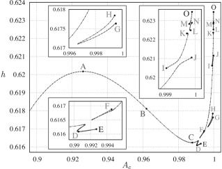
Figure 2: The bifurcation curve in Fig. 1 becomes fragmented in the range $0.985<A_{c}<1$, where previous numerical studies break down. The labels A–O correspond to wave profiles shown in Fig. 3. The turning point in wave steepness at C, the lack of monotonicity in $A_{c}$, the complicated branching structure, and the existence of standing waves with $h>0.62017$ were not previously known.

To compute standing waves, we use the Levenberg-Marquardt method Nocedal and Wright (1999), a trust-region algorithm for nonlinear least squares problems, to minimize

$$f(c)=\frac{1}{4\pi}\int_{0}^{2\pi}\Phi(x,T/4)^{2}\,dx,\qquad c\in R^{n+1},$$ (5)

where $c$ contains the period as well as the nonzero Fourier modes of the initial conditions; i.e., $T=c_{0}$ and

$$\hat{\eta}_{k}(0)=c_{|k|}\quad(k\text{ odd}),\quad\;\hat{\Phi}_{k}(0)=c_{|k|}\quad(k\text{ even}).$$ (6)

Here $k$ ranges from $-n$ to $n$, excluding 0, and $n$ is chosen to be close to $\frac{1}{4}M_{1}$, leaving the upper half of the spectrum of $\eta$ and $\Phi$ to be zero initially. A symmetry argument Mercer and Roberts (1992) shows that driving the velocity potential to zero at time $T/4$ with initial conditions of the form (6) leads to a standing wave with period $T$ and zero impulse. The method fails if $f$ reaches a nonzero local minimum.

We discretize (5) with spectral accuracy by redefining $f=\frac{1}{2}r^{T}r$, where $r\in\mathbb{R}^{m}$, $m=M_{\nu}$, and

$$r_{i}=\Phi(\xi_{\nu}(\alpha_{i}),T/4)\sqrt{E_{\nu}(\alpha_{i})/m},\qquad\alpha_{i}=2\pi i/M_{\nu}.$$

The square root comes from $dx=E_{\nu}(\alpha)\,d\alpha$. Typically, $4n\leq m\leq 10n$. To track families of solutions, one of the $c_{k}$ is chosen as a continuation parameter Keller (1987) and eliminated from the search space when minimizing $f$. When a turning point is detected in this $c_{k}$, we switch to a different one; see Ambrose and Wilkening (2010); Wilkening and Yu for details. The Jacobian $J_{ik}=\partial r_{i}/\partial c_{k}$ is computed by solving the linearization of (1) about the current solution to obtain $\frac{\partial}{\partial c_{k}}\Phi(x,T/4)$. This can be parallelized very efficiently Wilkening and Yu , dramatically increasing the resolution we are able to achieve.

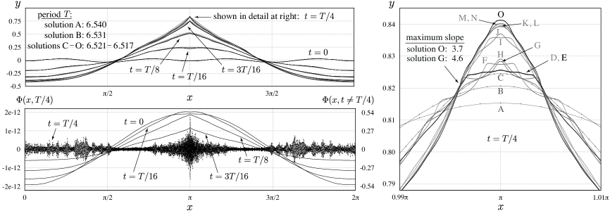
Figure 3: Evolution of standing waves and velocity potential over a quarter period. (Top left) Solutions A–O in Fig. 2 are plotted on top of each other at the indicated times. (Right) These solutions develop oscillatory structures near the crest that change phase across disconnections in the bifurcation diagram. Solutions D–O have 350–600 grid points between $0.99\pi$ and $1.01\pi$. With at most 3 grid points in this interval, previous numerical studies could not resolve these structures. (Bottom left) The velocity potential of solution O has been driven almost to zero at $t=T/4$, yielding $f=1.3\times 10^{-26}$. For this solution, we used $\nu=4$, $\theta_{l}=\{0.2,0.2,0.4,0.2\}$, $M_{l}=\{4608,6144,6912,8192\}$, $N_{l}=\{192,288,768,480\}$, and $A_{l}=\{0,0.774,1.358,1.381\}$.

Our results are summarized in Figs. 2 and 3. First, we corroborate the result of Mercer and Roberts Mercer and Roberts (1992) that wave steepness, $h$, reaches a local maximum of $h_{\text{max}}=0.62017$ at $A_{c}=0.92631$. (The values reported in Mercer and Roberts (1992) were $0.6202$ and $0.9264$.) Using quadruple precision, we are able to compute $h_{\text{max}}$ to 26 digits of accuracy and the corresponding $A_{c}$ to 13 digits. Okamura Okamura (2003), who found that $h$ increases monotonically all the way to $A_{c}=1$, was incorrect. Second, we find that crest acceleration has turning points at $A_{c}=0.99135$ and $0.99040$. This is a surprise, as $A_{c}$ was chosen as a continuation parameter in Mercer and Roberts (1992) to avoid the lack of monotonicity in $h$. In our work, $h$ and $A_{c}$ are plotted parametrically as functions of whichever $c_{k}$ is currently used as a continuation parameter. Finally, in the process of tracking this primary branch of solutions, we discovered several other families of standing waves. Each of these branches was tracked in both directions until the computations became too expensive to continue further with the desired accuracy, $f\sim 10^{-26}$ in double precision.

The standing waves that constitute these branches look qualitatively similar to each other in the large, where they closely resemble the photographs from Taylor’s wave tank experiments Taylor (1953). However, as illustrated in Fig. 3, solutions on different branches feature different oscillation patterns in the vicinity of the crest tip. The rapid increase in wave steepness from solution E to solution O in Fig. 2 corresponds to a vertical jet of fluid that forms near the crest before the standing wave reaches its rest state. The resulting protrusion causes the maximum slope to be much larger than 1 for most of these solutions. Taylor photographed similar structures at the crest in his wave tank experiments. Schultz et. al. Schultz et al. (1998) argued that surface tension was responsible for these protrusions, but we find that they occur even without surface tension. Comparing solutions A–E on the primary branch, we see that solutions eventually flatten out at the crest and become oscillatory rather than sharp. Figure 4 provides further evidence that these oscillations grow large enough to prevent this family of solutions from approaching a limiting wave profile in an asymptotically self-similar fashion.

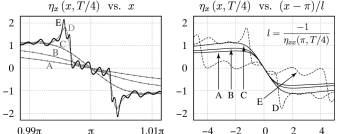
Figure 4: Breakdown of self-similarity on the primary branch. When lengths are rescaled so the radius of curvature at the crest is 1, the slopes of solutions A–C have similar shapes. In the traveling case (Fig. 5), these rescaled slopes would approach a limiting curve. But, for standing waves, oscillations develop, and a limiting curve does not emerge.

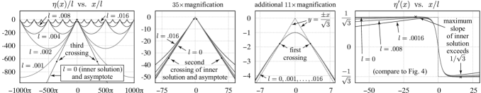
Figure 5: Self-similar asymptotics of traveling water waves near the wave crest. (Left) Using a variant of our standing wave code, we computed 5 periodic traveling solutions with wavelength $2\pi$ and particle speed $q$ at the wave crest, chosen so that $l=q^{2}/2g$ has the values shown. We then plotted $\eta(x)/l$ versus $x/l$, as well as the inner solution of Longuet-Higgins and Fox (1977). The distance between successive crossings of the inner solution with its asymptote grows exponentially; thus, $l$ must be extremely small to observe oscillatory behavior near the crest. (Right) As $l\rightarrow 0$, the slopes of the rescaled periodic waves approach the slope of the inner solution.

Regarding accuracy, our method is spectrally accurate in space, 8th or 15th order in time Wilkening and Yu , and quadratically convergent in the search for a minimizer of $f$ in (5). We achieve robustness by formulating the shooting method as an overdetermined nonlinear least squares problem. If the numerical solution loses resolution, the equations $r_{i}(c)=0$ become incompatible with each other and the objective function $f=\frac{1}{2}r^{T}r$ grows accordingly. This prevents the method from giving misleading overestimates of the accuracy of the standing waves it finds. For example, we recomputed solution O of Fig. 3 in quadruple precision on a finer mesh ($M_{l}=\{6144,7500,8192,9216\}$, $\theta_{l}=\{0.1,0.3,0.4,0.2\}$, and $A_{l}=\{0,1.043,1.405,1.476\}$), using the initial conditions obtained by minimizing $f$ in double precision. The more accurately computed value of $f$ is $8.6\times 10^{-27}$, which is 34% smaller than predicted in double precision. This level of inaccuracy in the predicted error is acceptable, as driving $\Phi(x,T/4)$ to zero entails eliminating as many significant digits as possible. For solution A, we repeated the minimization in quadruple precision, causing $f$ to decrease from $2.2\times 10^{-28}$ to $2.1\times 10^{-60}$. In addition to $f$, we monitor energy conservation and the decay of Fourier modes at various times to ensure that $\eta$ and $\Phi$ remain resolved to machine precision; see Wilkening and Yu for more details.

It is instructive to compare our results to the traveling wave case. Longuet-Higgins and Fox Longuet-Higgins and Fox (1977, 1978) showed that periodic traveling waves are asymptotically self-similar in two scaling regimes. If the wavelength, $L$, is held fixed as the crest tip sharpens, the limiting wave profile has a $120^{\circ}$ corner. This is the outer solution of Longuet-Higgins and Fox (1978), predicted by Stokes and proved to exist in Amick et al. (1982). If, instead, the fluid velocity at the crest remains fixed as the wavelength goes to infinity, the limiting wave profile is shown in Fig. 5. This inner solution crosses the asymptotes $y=\pm x/\sqrt{3}$ infinitely often Longuet-Higgins and Fox (1977), implying that traveling waves approach Stokes’s limiting wave in an oscillatory manner, rather than monotonically, with $L$ fixed.

The oscillations in the standing wave case are of a completely different nature. No choice of scaling will cause the curves in Fig. 4 to approach a limiting inner solution. We believe these oscillations are caused by resonant modes in the two-point boundary value problem (1) with boundary conditions $\Phi(x,\pm T/4)=0$, treating $T$ as a bifurcation parameter. A resonant mode is a perturbation that nearly satisfies the linearized boundary value problem. Such modes can be strongly excited in the process of computing standing waves, especially in finite depth Mercer and Roberts (1994); Smith and Roberts (1999); Wilkening and Yu . Disconnections in the bifurcation diagram seem to occur when a resonant mode can be excited with more than one amplitude. For example, solutions I and J in Fig. 3 both contain a secondary, higher-frequency standing wave (the resonant mode) superimposed on a low-frequency carrier wave. The secondary wave sharpens the crest at J and flattens it at I, being 180 degrees out of phase from one branch to the other.

We conclude that resonance is responsible for oscillations and trumps self-similarity in determining the dynamics of standing waves at small scales. This shows that, although under-resolved numerical simulations may exhibit self-similar dynamics, as happened in Okamura (2003), the true dynamics may be more complex. Recent work on singularity formation in free surface flow problems, such as droplet and bubble pinch-off Eggers and Fontelos (2009); Turitsyn et al. (2009) and wave breaking Bridges (2009), may also benefit from higher-resolution simulations, which could reveal new aspects of their dynamics.