The effect of local thermal fluctuations on the folding kinetics: a study from the perspective of the nonextensive statistical mechanics

Abstract

Protein folding is a universal process, very fast and accurate, which works consistently (as it should be) in a wide range of physiological conditions. The present work is based on three premises, namely: ($i$) folding reaction is a process with two consecutive and independent stages, namely the search mechanism and the overall productive stabilization; ($ii$) the folding kinetics results from a mechanism as fast as can be; and ($iii$) at nanoscale dimensions, local thermal fluctuations may have important role on the folding kinetics.

Here the first stage of folding process (search mechanism) is focused exclusively. The effects and consequences of local thermal fluctuations on the configurational kinetics, treated here in the context of non extensive statistical mechanics, is analyzed in detail through the dependence of the characteristic time of folding ($\tau$) on the temperature $T$ and on the nonextensive parameter $q$.

The model used consists of effective residues forming a chain of 27 beads, which occupy different sites of a $3-$D infinite lattice, representing a single protein chain in solution. The configurational evolution, treated by Monte Carlo simulation, is driven mainly by the change in free energy of transfer between consecutive configurations.

We found that the kinetics of the search mechanism, at temperature $T$, can be equally reproduced either if configurations are relatively weighted by means of the generalized Boltzmann factor ($q>1$), or by the conventional Boltzmann factor ($q=1$), but in latter case with temperatures $T^{\prime}>T.$

However, it is also argued that the two approaches are not equivalent. Indeed, as the temperature is a critical factor for biological systems, the folding process must be optmized at a relatively small range of temperature for the set of all proteins of a given organism. That is, the problem is not longer a simple matter of renormalization of parameters. Therefore, local thermal fluctuation on systems with nanometric components, as proteins in solution, becomes a important factor affecting the configurational kinetics.

As a final remark, it is argued that for a heterogeneous system with nanoscopic components, $q$ should be treated as a variable instead of a fixed parameter.

year number number identifier Date text]date

LABEL:FirstPage101 LABEL:LastPage#1102

I Introduction

Differently of most polymers, each natural protein folds over itself in a specific $3-$D structural conformation, its native structure. The series of events that drive a polypeptidic chain into its native structure, the folding process, is not yet fully understood: protein systems involve many complex interactions, and presents several remarkable properties that seems to require new experiments kumar , theoretical, and computational approaches dalmolin ; mok ; dill .

Although the folding process is surprisingly quick, folding rates $(K_{f})$ of different proteins can span several orders of magnitude ($K_{f}$ is a measure of how fast the folding process leads the chain from the unfolded state up to the native structure), and this remains true even for proteins of approximately the same size. Moreover, even for a single domain, two states, small proteins, existing theories for the kinetics of folding can not quantitatively predict this experimental observation plaxco –probably because the folding mechanisms have been routinely proposed from their ensemble-averaged properties, and from conflicting interpretation of its fundamentals rose1 ; rose2 .  Hence, the alternative ideas and hypotheses about folding explain only partially the phenomenon. For instance, the concept of transition state explain satisfactorily the two state kinetics but not the folding reaction rates, while that the funnel landscape idea can give insights about the folding rates but not for the two state kinetics Dill-a .

A remarkable characteristic of the folding process is its robustness, which can be illustrated by two intriguing properties: first, one finds that the folding is similarly processed in a large temperature range, covering about 100$\,{}^{\mathtt{o}}$C; and second, all functional proteins of all organisms, which live in the most different environments, fold correctly, and are stable about a particular ideal temperature. Indeed, living organisms are found in extreme conditions: some live in environments with temperatures near to freezing water piette ; Nicholas , while others are found in places with temperatures of boiling water wiggins ; zebb . Therefore, the search mechanism must work properly in the temperature interval from about zero to about 100 ^oC, while that for each alive species the range of functional temperature is in general relatively much smaller.

Proteins also present an extraordinarily precise and fast self-organization process. They fold some ten orders of magnitude faster than the predicted rate of a random search mechanism levinthal ; it is as if each protein had been designed to fold as fast as possible. Indeed, the probability of finding a fast-folding sequence, choosing it randomly from the set of all possible sequences, is very small gutin . However, there is also a physiological reason for fast folding: because do not have enough chaperone molecules to support folding of every protein (anyway chaperones also are proteins), they must fold very rapidly in order to avoid aggregation due to exposing hydrophobic areas of their surface for too long lorimer ; ecroyd .

Globular proteins can be considered as independent nanomachines. This particularity, in combination with the nature of most currently available experimental data, can be considered as one of the sources of certain inadequate views of the folding problem. The stable appearance and the properties of homogeneous macroscopic objects are resulting from the average activity of a very large number of atoms, but, contrasting with this scenario, nanostructures like colloidal particles or proteins, in contact with a thermal reservoir (the solvent), experience thermal fluctuations in a special way beck ; rajagopal . Actually, local unbalanced forces shake and deform continuously each of such nanostrucutures, which cannot be revealed by most of available data about protein kinetics that just reflects the collective behavior of a huge number of them in dilute aqueous solutions. That is, the result is a kind of temporal averaged view of the phenomenon. Nevertheless, new data and ideas start to emerge from single molecule experiments kumar , such as about transition paths at equilibrium –which is only observable for single molecules, allowing to obtain crucial mechanistic information, for instance, folding and unfolding rates Eaton .

Part of such general properties may be better understood if one considers that the search mechanism is governed mainly by the hydrophobic effect, whose strength, as shown experimentally at least for small hydrophobic molecules chandler ; luiz , varies slightly in the temperature interval from about zero to 100 ^oC. Therefore, it is suggested that folding process should be composed of two temporal steps eulalia : the search mechanism, as the first stage, followed by the overall stabilization that only begins with the chain close enough to its native conformation, when energy and structural requirements, as encoded in the residue sequence, would be associated in a productive and cooperative way.

Based in these general properties, a few hypotheses can be formulated; therefore we assume as general grounds for the folding problem, the following three statements:

$(i)$- the complete folding process is composed by two timely independent steps, namely: the search mechanism, and the overall productive stabilization.

$(ii)$- for typical one domain, two state globular proteins the folding instructions encoded in the residues sequence provide a folding kinetic as fast as possible; and

$(iii)$- at nanoscale dimensions randomness emerges as a peculiar attribute of the protein molecule, which should be treat individual and appropriately with respect to the effects of local thermal fluctuations.

Our goal in this work is to show evidences concerning the importance of local thermal fluctuations on the kinetics of the folding process of globular proteins. The simplified model employed here (next section) focuses exclusively on the search mechanism and have as its grounds the hydrophobic effect. Fluctuation effects on a nanoscale structure are treated in the context of the nonextensive statistical mechanics (section III), and are analyzed in details through the dependence of the folding characteristic time $\tau$ on the temperature $T$ and nonextensive parameter $q$ (section IV). The behavior of small, single-domain globular proteins are used here as ideal prototypes; usually many of them fold via an all-or-nothing process, that is, without detectable intermediates jackson . Comments and conclusions (section V) are formulated according the three hypotheses stated above.

II The model

The model presented here is based on the first hypothesis, stated in previous section. It is devoted just for the first stage of the folding process, the search mechanism, in order to explore general aspects of the folding problem valid, in principle, for all proteins. Therefore a lattice model is used: effective residues (a chain of 27 beads), occupying consecutive and distinct sites of a three-dimensional infinity cubic lattice, represent a single protein-like chain in solution; effective solvent molecules, which explicitly interact with the chain, fill up the lattice vacant sites. The general scheme to explore the configurational space presumes that, during the simulation, solvent molecules and chain units exchange their respective sites so that all sites of the lattice remain always fully filled eulalia ; roosevelt .

For each configurational change, only the transfer free energy (variations on the hydrophobic energy) is taken into account –given that the model is conceived to deal specifically with the search mechanism; solvent-solvent and residue-residue interactions are represented by hard core-type interactions (excluded volume). For a regular cubic lattice, which in the present case means uniform solvent density, this interaction scheme is exactly equivalent to the use of additive, first neighbor, inter-residue pairwise potentials, namely $h_{i,j}=h_{i}+h_{j}$, where $h_{i}$ is the hydrophobic level of the $i^{th}$ residue in the chain sequence luiz2 . Residues are taken from a repertory of ten distinct units (a ten-letter alphabet), which are characterized by distinct hydrophobic levels and a set $\{c_{i,j}\}$ of inter-residue steric specificities. The hydrophobic levels has been considered the most general and influential chemical factor acting along the folding process li , while the set of inter-residues constraint mimics steric specificities of the real residues. These specificities are achieved through the specification of which pairs of residues are allowed to get closer, as first neighbors, and its main consequence is to select folding and unfolding pathways through the configurational space. The set of inter-monomer constraints is fixed for each monomer pair, that is, it does not depend on the particularities of the native structure dalmolin ; eulalia .

The configurational energy $E([\kappa,l])$ of an arbitrary chain configuration $\xi$ defined by the set $[\kappa,l]$ of $N_{\xi}$ first neighbor inter-residue contacts $(0\leq N_{\xi}\leq 28)$ is

$$E([\kappa,l])=\sum_{\{i,j\}}(h_{i,j}+c_{i,j})\delta_{(i,j),[\kappa,l]},$$ (1)

where the sum runs over the set of all residues pairs $\{i,j\}$; the factor $\delta_{(i,j),[\kappa,l]}=1$ if $(i,j)$ belongs to the set $[\kappa,l]$; otherwise $\delta_{(i,j),[\kappa,l]}=0$.

The present model is not native-centric, that is, data from the native structure are not employed to guide the chain along the simulation. Consequently, a rule for sequence designing, valid for any target structure –representing the native structure, is necessary. The provided syntax is mainly based on the hydrophobic inside rule dill2 and on the local topological features of the target structure roosevelt ; tese .

Models based on this stereochemical potential has been proved to be efficient in packing the chain and finding the native state ines , but they fail to provide stability to the native state because such additive potential, $h_{i,j}=h_{i}+h_{j}$, satisfies marginally the segregation principle (namely, $2h_{i,j}+h_{i,i}+h_{j,j}\leq 0$) through the equal sign, that is: $2h_{i,j}+h_{i,i}+h_{j,j}=0$. However, adding up steric constraints $\{c_{i,j}\}$ to the hydrophobic potential $h_{i,j}$, as in Eq.(1), some important consequences are observed: for instance, it helps to select folding and unfolding pathways, which makes faster the folding process, and improves the overall stability condition of the globule in the native state eulalia .

The folding process is simulated through the Metropolis Monte Carlo (MC) method, involving standard elementary chain moves, namely: crankshaft, corner, and end flips. For each move attempt, a particular reference point along the chain is chosen at random and the process evolves without any reference to the native configuration, except to check when it is found for the first time: for each particular run, the number of MC-steps spent to reach the native structure from the initial configuration (the first passage time) is took as the folding time $t$ for that case.

III Local thermal fluctuations and the nonextensive statistical mechanics

Usual thermodynamic and kinetic data about proteins are time-averaged results from the collective behavior of many molecules, something between$~{}\sim 10^{17}-10^{20}$ molecules/litter. This condition determines the traditional tendency to view globular proteins as mostly compact and static structures. However, when considered individually, proteins surely undergo strong fluctuations in their thermodynamic properties. For instance, let us reproduce here a specific thermodynamic calculation cooper for a system constituted by a representative protein of about $250$ residues in solution,  with molecular mass $m$ about $4\times 10^{-23}$ kg that typically shows heat capacity $(C_{p}\cong C_{v})$ about $0.3$ kcal kg^-1K^-1, at temperature $T=300$K. A simple estimate of the internal energy fluctuation about the mean, for an individual molecule, gives $\Delta U_{rms}\cong 6\times 10^{-20}$ cal per molecule $(\Delta U_{rms}=kT^{2}mC_{V})$. Essentiality, it would be in the same order of magnitude of the typical enthalpy changes on thermal denaturation of proteins –tens of Kcal/mol privalov – if all molecules were fluctuating in concert cooper . Actually, fluctuations are individually uncorrelated: in a population with a huge number of macromolecules, fluctuations tend to cancel each other, producing thermodynamic parameters well behaved.

However, for each single protein such fluctuations may interfere in the folding kinetics in one way or another; therefore the folding process has to be explained for each single molecule. Let us then think about a protein in solution as a heterogeneous system constituted by just one chain in its solvent, which works as a heat reservoir at macroscopic temperature $\beta_{0}^{-1}$. But, due to the protein nanosize scale, it is as if the temperature were locally fluctuating. Then, if (locally) $\beta^{-1}$ fluctuates rapidly with respect to the typical time spent for chain configurational interchanges, one could think about a generalized Boltzmann factor exp${}_{q}(-\beta_{0}\epsilon)$ as an integral over all possible locally fluctuating $\beta^{-1}$, that is

$$\mathrm{exp}_{q}(-\beta_{0}\epsilon)=\int_{0}^{\infty}\mathrm{exp}(-\beta\epsilon)f(\beta)d\beta.$$ (2)

It has been shown that if $f(\beta)$ is assumed to be the $\chi^{2}$-distribution, a special case of the gamma-distribution of variable $\beta$, present in many common circumstances hastings , the generalized Boltzmann factor becomes beck ; rajagopal ; touchette

$$\mathrm{exp}_{q}(-\beta_{0}\epsilon)=[1-(1-q)\beta_{0}\epsilon]^{\frac{1}{1-q}},$$ (3)

which is the same expression proposed in the context of nonextensive statistical mechanics tsallis1 ; tsallis2 . The $\chi^{2}$-distribution

$$f(\beta)=[\Gamma(n/2)]^{-1}\left(\frac{n}{2\beta_{0}}\right)^{n/2}\beta^{-1+n/2}\exp\left(-\frac{\beta}{2\beta_{0}}n\right)$$ (4)

is parameterized such that the heat reservoir temperature $\beta_{0}^{-1}$ coincides with the average of the fluctuating $\beta$, that is: $\beta_{0}=\langle\beta\rangle=\int_{0}^{\infty}\beta f(\beta)d\beta$ . The nonextensive parameter $q$, set as

$$q=1+2/n,$$ (5)

is associated with the relative dispersion of $\beta$, according $q=1+(\langle\beta^{2}\rangle-\beta_{0}^{2})/\beta_{0}^{2}$, where $n$ is the number of degrees of freedom. This point will be returned later in the next section.

In the present work our interest is mainly concerned with the kinetic behavior of the chain during the folding process, starting from a open configuration until to reach its native conformation. Therefore, for MC realizations we assume a generalized transition probability exp${}_{q}(-\beta_{0}\Delta\epsilon_{ab})=\langle$exp$(-\beta_{0}\Delta\epsilon_{ab})\rangle$ between the configuration $a$ with energy $\epsilon_{a}$, and configuration $b$ with energy $\epsilon_{b}$, that is,

$$\mathrm{exp}_{q}(-\beta_{0}\Delta\epsilon_{ab})=[1-(1-q)\beta_{0}\Delta\epsilon_{ab}]^{\frac{1}{1-q}}$$ (6)

where $\Delta\epsilon_{ab}=\epsilon_{b}-\epsilon_{a}$ .

For $q\gtrsim 1$ the $q$-exponential and the conventional exponential function behave in a very similar way, that is, one may expect that exp${}_{q}(-x)$ is effectively equivalent to the conventional exponential function in which its argument has been adequately changed (that is, with the temperature increased somewhat). Actually, comparing the two following difference functions, namely $\Delta_{q}(x)=\exp_{q}(-x)-\exp(-x)$ and $\Delta_{a}(x)=\exp(-ax)-\exp(-x)$, as shown in Figure 1 for $a$ and $q\cong 1$ , one sees that their profiles are similar, although the maximum of $\Delta_{a}(x)$ occurs about $x_{a}=1,$ and for $\Delta_{q}(x)$ it is about $x_{q}=2$. Actually, the $\lim_{a\rightarrow 1}(x_{a})=1,$ while $\lim_{q\rightarrow 1}(x_{q})=2$; in both cases $x_{a}$ and $x_{q}$ increases slowly when $a$ decreases from one and $q$ increases from one.

Therefore we compare the effect of both approaches on the configurational kinetics through MC simulation, and then discuss possible implications for the understanding of the folding mechanism. In order to address directly this issue, we consider the folding time $t$ and the folding characteristic time $\tau$ (described in the next section) as analytical amounts emerging from the folding kinetics. The comparison between the two approaches emphasizes the effects of local fluctuations in a heterogeneous system (with nanosized scaled components) through the view of the nonextensive statistical mechanics.

IV Results and Discussion

The characteristic folding time $\tau$ is determined by means of a sample of many folding trajectories, that is for each target (native) structure a number $N$ of independent runs represents the folding process of a set of $N$ non-interacting proteins (diluted solution). For each run, say the $i^{th}$ run, the MC time $t_{i}$ spent to find the native structure (first passage time) is adopted as the folding time for that case. So, at the end of $N$ independent runs one gets a set $\{t_{i}\}_{N}$ of independent folding times and then, by counting the number of folding times that fall in each time interval $[t,t+\Delta t]$ one finally gets the decay histogram of the number of unfolded proteins as a function of the MC time $t$. These data are then fitted by one (or more) exponential function, giving the specific characteristic folding time $\tau$ for that structure. The simulations are carried out in a given range of temperatures $T$ for several values of the nonextensive parameter $q$, and for distinct native structures. Each native structure is characterized by their topological complexities, which can roughly be estimated by its structural Contact Order plaxco1 ; ines .

As an encompassing survey, Table $1$ shows $\tau$ in function of the temperature $T$ and nonextensive parameter $q$, in the interval $0.9\leq T\leq 1.5$ and $1\leq q\leq 1.4$. Three representative target (native) structures (identified as ID 866; 1128 and 36335) were used; in general, $\tau$ depends on the structure complexity, and is a continuous, convex function of $T$ and $q$. A total of $N=150$ independent runs were used for each pair $(T,q)$. The structure ID 36335 presents higher topological complexity than the others two, a fact reflected in its larger $\tau$.

For any temperature $T_{i}$, there is a specific $q_{i}=q(T_{i}),$ let us say $q_{i}^{\ast},$ that minimizes $\tau$, that is $\tau\rightarrow\tau_{\min}$, as emphasized in Table $1$ by shaded cells; better approximations can be achieved by extra refinement of $q$.  The uncertainty in $\tau$ was estimated by the standard deviation of the mean of means, considering $20$ distinct samples $\{t_{i}\}_{N}$ $($with $N=150)$ taken from an extended set of $10^{4}$ independent runs. The uncertainty $\delta\tau$ depends on the pair $(T,q);$ the smallest uncertainties $(\simeq 5\%)$ occur for those specific values $q_{i}^{\ast}$ which minimize the characteristic folding time $\tau\cong\tau_{min}$. On the other hand, when the system approaches the glassy regime ($T<<1)$ the time spent in metastable states increases substantially, and so $\delta\tau$ is strongly influenced by the size $N$ of the set $\{t_{i}\}_{N}$ of independent runs.

This scenario suggests that the kinetic of the search mechanism is equally reproduced, not mattering if the configurations are relatively weighted by mean of the generalized Boltzmann factor, namely, $\exp_{q}(-\Delta\epsilon/kT)$ (see Eq. (3)), or by the conventional Boltzmann factor, $\exp(-\Delta\epsilon/kT^{\prime}~{}),$ with the system temperature $T^{\prime}$ increased by some amount with respect to $T$. This can be seen clearly if, for each $q,$ the behavior of $\tau$ is plotted as a function of the translated temperature scale $\mathcal{T}_{q}=T-T_{q}^{\ast}$, as shown in Figure 2 for structure ID 1128; $T_{q}^{\ast}$ is the temperature in that $\tau$ approaches $\tau_{\min}$ for that value of $q$. Essentially all curves behave in the same way about $\mathcal{T}_{q}=0.$

A more detailed examination shows that the distributions $\Phi$ of folding times are essentially the same in both approaches, that is, using $\exp_{q}(-\Delta\epsilon/kT)$  or $\exp(-\Delta\epsilon/kT^{\prime}).$ Figure 3  shows $\Phi=\Phi(T)$ for structure ID $866,$ for different values of $q$; much more independent runs $(N=10^{4})$ were employed for each case. In general, the distributions are better fitted with one or more lognormal curves, depending on the temperature.

For $(q,T)=(1,1)$, the system approaches the glassy regime with manifestation of ergodic difficulties, as indicated by the three peaked curve; Figure 3, open, smaller circles. As $T$ increases from $T=1,$ the domain of $t$ is accordingly reduced; at $T\cong 1.5$ the distribution presents the smallest domain, namely $0<\ln(t)<5.5$, and as $T$ increases from this point its behavior is reverted: the size of the domain starts to increase again and the curve’s peak moves in the direction of larger $t$. In the region of the smaller folding times, namely for $\ln(t)<2.5$, all curves present the same behavior, if $T$  is restricted in the interval $1.2\leq T\leq 1.5$. The meaning for this is: even with the temperature 25% higher than $T=1.2$, there exist some configurations among the initial open ones, which combined with certain configurational evolution, can lead the chain very rapidly into the native structure. Note that this is also true for the case $(q,T)=(1.1,1.0).$

The frequency distribution $\Phi=\Phi(T)$ for $(q,T)=(1.1,1.0)$ (open large circles –generalized Boltzmann factor) is practically the same as that for $(q,T)=(1.0,1.25)$ (full smaller circles –conventional Boltzmann factor ), implying in the convergence of the folding characteristic time for the two cases, namely, $\tau_{\min}=24$ (see Table $1$ and Figure 3). This result confirms that (for the present problem) the net effect of the generalized Boltzmann weight on the kinetic of the search mechanism is equivalent, from the perspective of the conventional Boltzmann factor, to a specified increase in the system temperature, that is, a certain increase on thermal fluctuations. So, a specific well tuned amount of thermal fluctuation is what determines the fastest folding process. Then, independent of the approach (generalized or conventional Boltzmann factor), and according the hypothesis that the folding instruction encoded in the residue sequence provides a folding kinetic as fast as possible (Section II, second premise), $\tau_{\min}$ is adopted as the optimum $\tau,$ the actual characteristic folding time.

However, due mostly to the peculiarities of protein systems, the folding process must be minimaly optimazed in a relatively narrow range of temperature, and for the total set of proteins of each living organism.  In this sense the two approaches are not equivalent: the fact that each target structure has a proper temperature for fastest folding could be seem as a model deficience that should be improved by approaching the problem by the nonextesive statistical mechanics. Moreover, as already mentioned, the search mechanism operates equally in large temperature interval, but, once the native structure is found, the other stage of the folding process takes place –the overall productive stabilization, which is strictly dependent on the temperature. Indeed, for the set of protein of each organism there is a working temperature interval $T_{\omega}-\Delta T\lesssim T\lesssim T_{\omega}+\Delta T$  (with $\Delta T/T_{\omega}\lesssim 20\%),$ outside of which its functionality can be seriously reduced or completely lost. Therefore, the system temperature $T$ must be kept as the reference temperature, measured macroscopically, and all thermal characteristics of a nanosize body, in response to the local thermal fluctuations, should be conveniently controlled by the nonextensive parameter $q$.

For any target structure, at specific system temperature $T$, it is always possible to adjust $q$ in order to get the optimum $\tau$. But, what intrinsic factors would determine a specific $q^{\ast}$ value that induces the fasted folding for that specific protein? In the present case, namely a chain evolving through the configurational space from a open chain into a compact specific globule, the straightforward idea comes from the observation that local fluctuations of $\beta$ should be dependent on the spatial scale beck1 ; beck2 . Indeed, along the simulation specific traps as well wrong packing tendency are recurrent, and so the resulting effect of local thermal fluctuations is to promote a rich variety of shape and size of the globule. To see this argument in more details, let each residue of the chain be associated, as upper bound, to just one degree of freedom, which allow us to explore the relation between $q$ and the numbers of degrees of freedom $n$ of the system: $q=1+2/n$, Eq. (4) and (5). Through this relation we may recognize a subtle association between $q^{\ast}$ and the topological complexity of the native structure. One notes, firstly, the dynamic nature of the number of degrees of freedom $n$: as the chain degree of compactness changes in the course of the time, $n$ changes accordingly. So, for an open chain we have $q_{\min}=1+2/n_{\max}\rightarrow 1$, and for a fully compact globule $q_{\max}=1+2/n_{\min}$. Using $n_{\min}=1$ as a limiting condition, one gets a kind of upper bond for $q$, that is, $q_{\max}=3$. Actually, along the folding process, energy and topological traps must be overcome until the target structure is reached. Such recurrent traps keep the chain for relatively long time in wrong conformations of different degrees of compactness, which must be disassembled so that the folding process can be restarted. Therefore, as the chain suffers the thermal effects differently, depending on its compactness, the simulation process should be governed by a variable instead of a fixed parameter $q$. However, depending on the number of traps and their peculiarities –determined by the combination of the complexity of the native structure and the chain sequence, a specific $q^{\ast}$ (kind of average $q$) may be associated to each target structure; this is what we did in this work and is showed in Table $1$ for three different target structures. Clearly, a direct inspection of this process can be carried out using a dynamic process that changes (appropriately) the value of $q$ along the simulation. The implementation of this idea is now in progress.

V Final Comments and Conclusions

The hypotheses about the folding reaction as a two independent stages (search and stabilization) enabled us to place emphasis just on the search mechanism as an universal process guided by the hydrophobic force, which performs equally in a large range of temperatures. The premise about the fastness of the folding process (necessary to prevent protein aggregation) was used in order to associate the nonextensive parameter $q^{\ast}$ to each native structure.

The comparison between the two approaches, namely the nonextensive $(~{}q>1)$ and the conventional $(q=1)~{}$statistical mechanics, suggests that suitable thermal fluctuations –adequately achieved only in the nonextensive context– drives the chain through the fastest possible courses to the native conformation, as shown in Figure 2. The generalized Boltzmann factor  has a qualitatively equivalent effect with respect to the conventional Boltzmann factor, that is, to enlarge the chance of removing the chain from energetic or topological traps. Although their extremum effects on the transition probabilities between two consecutive configurations are energetically shifted (Figure 1), appropriate combinations of $T$ and $q,$ such as $(T=1;q>1)$ and $(T^{~{}\prime}>1;q=1),$ for example, can produce practically the same folding time distribution $\Phi$ (Figure 3), determining the same optimum characteristic folding time $\tau_{\min}.$

The well known U–shape dependence of $\tau$ on temperature, shown in Figure 2, has been commonly attributed exclusively to peculiarities of the chain sequence –or to the complexity of the target structure. Indeed, sequences are usually generated and tested for its ability to fold rapidly in an small and specific range of temperature Karplus-a , even knowing that this procedure eliminates many suitable structures that would otherwise be important for kinetic studies. But a new perspective emerges when local thermal fluctuations experienced by nanoscale structures is associated with its spatial characteristics (as its size and degrees of freedom), by means of the parameter $q$  from the nonextensive statistical mechanics. Specifically, such as chaperone that assists the folding, well tuned thermal fluctuations help to disassemble chain segments wrongly collapsed, improving the fastness of the folding process; otherwise, using the conventional statistic mechanics, it would be achieved only at higher temperature of the reservoir. Therefore, extending this scenario to real protein systems we may visualize the two main driving forces (entropic forces compacting the chain and local thermal fluctuations tending to open it) suporting a continuous process of folding/unfolding until, eventually, the neighborhoods of the native state is reached. At this point, and only under this condition, the native structural peculiarities and chain energetic interactions, as encoded along the chain sequence, would be associated in a cooperative and fully productive way, guarantying the globule overall stability.

As a final remark, we recall that the exploratory analysis summarized in Table 1 suggests that $q$ increases with the topological complexity of the target structure. Indeed, treating $q$ as a variable, let us say $\mathbf{q}$, we get essentiality the same result, that is: the characteristic time $\tau$ converges to the same $\tau_{\min}$ obtained using $q=q^{\ast}$ as a parameter. In a preliminary investigation, $\mathbf{q}$ was functionally linked to the instantaneous radio of gyration, which was used as a measure of the chain compactness (degrees of freedom). Accordingly, for each of several distinct target configurations investigated, the resulting $\mathbf{q}$-distribution is characterized by one or two peaks around the constant $q=q^{\ast}$ used as a parameter.

Acknowledgements

We thank Dr. Alexandre S. Araujo for reading our manuscript, and CNPq for funding.

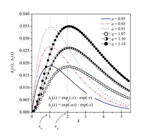
Figure 1: Functional difference between the generalized and the ordinary exponential function, namely $\Delta_{q}(x)=\exp_{q}(-x)-\exp(-x)$, with $q\gtrsim 1,$ and between two ordinary exponential functions with the argument of one of them rescaled, that is: $\Delta_{a}(x)=\exp(-ax)-\exp(-x),$ with $a\lesssim 1$; the parameter $a$ represents a small increment in the system temperature. Their profiles are similar but, for $a$ and $q$ near to $1,$ the maximum of $\Delta_{a}(x)$ and $\Delta_{q}(x)$occur about $x_{a}=1$ and $x_{q}=2$, respectively.  In both cases, $x_{a}$ and $x_{q}$ increases very slowly when $a$ and $q$ depart from 1.

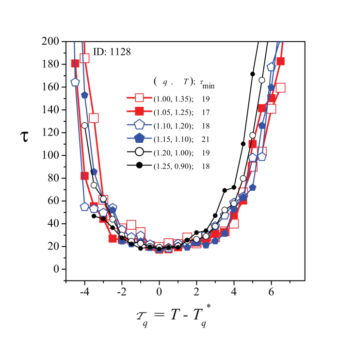
Figure 2: The $\tau\times T$  ”U–shape ” : folding characteristic time $\tau$ as a function of the translated temperature $\mathcal{T}_{q}=T-T_{q}^{\ast}$  for several $(q,T)$ combinations. $T_{q}^{\ast}$ is the temperature in that $\tau=\tau_{\min}$ for that value of $q$. For each $q$, the temperature range was covered by increments $\Delta T=0.05.$ All curves behave very similarly around $\mathcal{T}_{q}=0$.

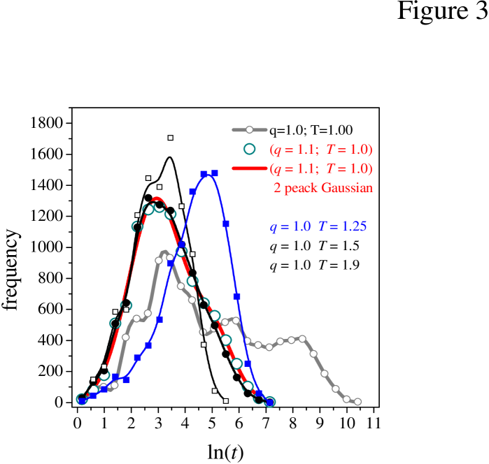
Figure 3: Folding time distributions $\Phi$ for structure ID 866. The lognormal distribution for $q=1.1$ and $T=1.0$   (larger open circles) was fitted using two peaks Gaussian (continuous thicker line – amplitude: ($A_{1};\,A_{2})\,=(1310\pm 40;430\pm 70)$; width ($w_{1};$ $w_{2})=(0.49\pm 0.07;0.8\pm 0.3)$, and average $(\mu_{1};\mu_{2})=(2.91\pm 0.09;5.0\pm 0.2))$. For $q=1.0$ the folding time behavior is shown for several temperatures (fitted by basic spline functions). In particular, the folding time distribution for $(q,T)=(1.0,1.25)$ and $(1.1,1.0)$ are practically the same, confirming that the generalized Boltzmann factor $(q>1)$ at temperature $T$, corresponds to the conventional Boltzmann factor $(q=1)$ with a certain increase in $T$. In the region of the smaller folding times $(\ln(t)<2.5)$ and for temperatures in the interval $1.0\leq T<1.5$, all curves coalesce –including the case $(q,T)=(1.1,1.0)$. At $T=1.0$ and $q=1$ (full gray circles) the system approaches the glassy regime and manifestation of ergodic difficulties are evident. At temperature $T=1.5$ the distribution has the lowest domain, that is, $0<\ln(t)<5.5$ (open squares), and inasmuch as $T$ increases from this point, the peak of the distribution moves again toward larger $t$, as illustrated for $T=1.9$ (full squares).

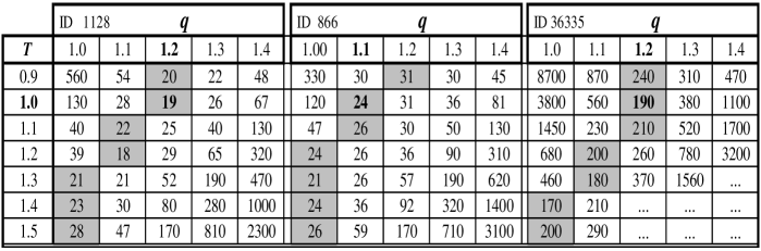
Figure 4: Table 1 – Characteristic folding (MC) time $t$ for three target (native) structures; the unit MC time used here corresponds to 8100 attempts to move the chain. For each structure and temperature $T_{i}$ there is a specific $q=q(T_{i})\geq$ 1 that minimizes $\tau$ (shaded cells). Due to the higher topological complexity of structure ID 36335, its $\tau$ is 5 to 10 times larger than the corresponding values of $\tau$ for the others two structures. A set of $N=150$ independent runs was used to estimate $\tau$ for each pair $(T,q)$. The figures were rounded off according to average relative uncertainty $\delta\tau=10\%$ (two significant figures); see text. At $T=1$, the values for $q$ that give the smallest folding characteristic times are generally depending on the complexity of the corresponding native structure –shaded cells, bold figures.

References

- (1) Sanjay Kumar, Mai Suan Li, Physics Reports, 486 1 (2010).
- (2) J. P. Dal Molin, Marco Antonio Alves da Silva, I. R. da Silva, and A. Caliri, Braz. J. Phys. 39(2A), 435 (2009).
- (3) K. H. Mok, L. T. Kuhn, M. Goez, I. J. Day, J. C. Lin, N. H. Andersen, P. J. Hore, Nature 447, 106 (2007).
- (4) K.A. Dill, S.B. Ozkan, M.S. Shell, T.R. Weikl, Annu. Rev. Biophys. 37, 289 (2008).
- (5) B. Gillespie, K. W. Plaxco, Annu. Rev. Biochem. 73, 837 (2004).
- (6) G. D. Rose, P. J. Fleming, J. R. Banavar, Amos Maritan, Proc. Natl. Acad. Sci. USA, 103(45), 16623 (2006).
- (7) D. W. Bolen, G. D. Rose, Annu. Rev. Biochem., 77 339 (2008).
- (8) Jack Schonbrun and Ken A. Dill, Proc. Natl. Acad. Sci. USA, 100(22), 12678 (2003).
- (9) F. Piette, S. D’Amico, C. Struvay, G. Mazzucchelli, J. Renaut, M. L. Tutino, A. Danchin, P. Leprince, G. Feller, Molecular Microbiology, 76(1), 120 (2010).
- (10) Nicholas J. Russel, Extremophiles 4, 83 (2000).
- (11) P. Wiggins, PLoS ONE, 3(1), e1406 (2008).
- (12) M. Zeeb, G. Lipps, H. Lilie, J. Balbach, J. Mol. Biol., 336, 227 (2004).
- (13) C. Levinthal, J. de Chim. Phys., 65(1), 44 (1968).
- (14) A. M. Gutin, V. I. Abkevich, E. I. Shakhnovich, Proc. Natl. Acad. Sci. USA, 92(5), 1282 (1995).
- (15) G. H. Lorimer, FASEB J, 10, 5 (1996).
- (16) H. Ecroyd, J. A. Carver, IUBMB Life, 60(12), 769 (2008).
- (17) C. Beck, Europhys. Lett., 57(3), 329 (2002).
- (18) A. K. Rajagopal, C. S. Pande, S. Abe, Nano-Scale Materials: From Science to Technology, pages: 241-248 (2006) - Workshop on Nano-Scale Materials - From Science to Technology; APR 05-08, 2004 Puri INDIA.
- (19) H. S. Chung, J. M. Louis, and W. A. Eaton, Proc. Natl. Acad. Sci. USA, 106(29), 11837 (2009).
- (20) D. Chandler, Nature 417, 491 (2002).
- (21) L.F.O. Rocha, M.E. Tarragó Pinto, and A. Caliri, Braz. J. Phys. 34(1), 90 (2004).
- (22) M.E.P. Tarragó, L.F.O. Rocha, R.A. da Silva, A. Caliri, Phys. Rev. E 67, 031901-1 (2003).
- (23) S. E. Jackson, Fold. and Des., 3 81 (1998).
- (24) R.A. da Silva, M.A.A. da Silva, A. Caliri, J. Chem. Phys. 114(9), 4235 (2001).
- (25) L. F. O. Rocha, I. R. Silva, A. Caliri, Physica A, 388 4097 (2009).
- (26) H. Li, C. Tang, and N. S. Wingreen, Phys. Rev. Lett. 79, 765 (1997).
- (27) K. A. Dill, Biochemistry 29, 7133 (1990).
- (28) I. R. da Silva, PhD Thesis, http://www.teses.usp.br/teses/disponiveis/59/59135/tde-24082005-112844/ in Portuguese (2005).
- (29) I.R. Silva, L.M. dos Reis, A. Caliri, J. Chem. Phys. 123(15), 154906-1, (2005).
- (30) A. Cooper, Proc. Natl. Acad. Sci. USA, 73(8), 2740 (1976).
- (31) P. L. Privalov, in Protein Folding, ed. by T.E. Creighton, W.H. Freeman and Company, New York, chapter 3, (1992).
- (32) N. A. J. Hastings, J. B. Peacock, Statistical Distributions, John Wiley & Sons INC, New York (2000).
- (33) H. Touchette, in Nonextensive Entropy: Interdisciplinary Applications, ed. by M. Gell-Mann, C. Tsallis, Oxford University Press, (2004).
- (34) C. Tsallis, J. Stat. Phys. 52, 479 (1988).
- (35) C. Tsallis, Introduction to Nonextensive Statistical Mechanics, Springer, (2009).
- (36) K. W. Plaxco, K. T. Simons, D. Baker, J. Mol. Biol., 277, 985 (1998).
- (37) C. Beck, G. S. Lewis, H. S. Swinney, Phys. Rev. E, 63, 035303, (2001).
- (38) C. Beck, Phys. Rev. Lett., 87, 180601 (2001).
- (39) A. R. Dinner, A. Sali, and M. Karplus, Proc. Natl. Acad. Sci. USA, 93, 8356 (1996).