Analytic Harmonic Approach to the $N$-body problem

Abstract

We consider an analytic way to make the interacting $N$-body problem tractable by using harmonic oscillators in place of the relevant two-body interactions. The two-body terms of the $N$-body Hamiltonian are approximated by considering the energy spectrum and radius of the relevant two-body problem which gives frequency, center position, and zero point energy of the corresponding harmonic oscillator. Adding external harmonic one-body terms, we proceed to solve the full quantum mechanical $N$-body problem analytically for arbitrary masses. Energy eigenvalues, eigenmodes, and correlation functions like density matrices can then be computed analytically. As a first application of our formalism, we consider the $N$-boson problem in two- and three dimensions where we fit the two-body interactions to agree with the well-known zero-range model for two particles in a harmonic trap. Subsequently, condensate fractions, spectra, radii, and eigenmodes are discussed as function of dimension, boson number $N$, and scattering length obtained in the zero-range model. We find that energies, radii, and condensate fraction increase with scattering length as well as boson number, while radii decrease with increasing boson number. Our formalism is completely general and can also be applied to fermions, Bose-Fermi mixtures, and to more exotic geometries.

1 Introduction

Determining the ground state and properties of $N$ interacting particles in some fixed geometry is at the core of many disciplines in physics and other natural sciences. However, in general even for moderate values of $N$, methods based on first principles are either intractable or extremely time-consuming. Fortunately, the properties of many systems can be described by correlations that involve just a few particles and the problem of many particles can be reduced to consider a much smaller number in the background of the remaining particles. Two-body interactions still have a tendency to make even such few-body problems very difficult to solve and insights gained from approximations that allow analytic treatments are therefore very useful.

In configuration interaction methods, where large basis states of properly symmetrized wave functions are built and diagonalized to determine system properties, a basis of harmonic oscillator states can be very convenient as matrix elements of the two-body interaction are easy to calculate. This approach was used early on in the context of the nuclear shell model [1, 2]. Turning this method upside down the potentially complicated two-body interaction could be reproduced or simulated by a simple harmonic oscillator potential. The great advantage is obviously that the coupled set of differential equations of motion are much simpler to solve, and a number of properties are easily systematically obtained as functions of interaction parameters and particle number.

In subfields of physics where the structure is already established at a given level of accuracy, the insight gained from oscillator approximations is most often insufficient for improvements. However, in cold atomic gas physics it is now possible to prepare systems with very exotic and often unknown properties, to use controlled two-body interactions, to study different geometries and dimensions, and to vary trapping conditions [3]. Analytical oscillator approximations can therefore be expected to be very valuable, as it has been in other fields of physics. While we are concerned mainly with the quantum mechanical many-body problem here, we note that similar techniques are currently used also in the study of classical dynamics [4].

Obviously, the accuracy of the oscillator approximation increases as the potentials resemble oscillators. This means that pronounced smooth potential single minima with room for bound states are directly suited for investigations of system structures as functions of particle number and other characteristics. However, also much weaker binding potentials would reveal correct overall qualitative, and perhaps also semi-quantitative, behaviour in an appropriate oscillator approximation. This is especially emphasized by the universal behaviour of a number of weakly bound structures which only depend on integral properties like scattering length. In that case, the bulk part of the potentials are not crucial by themselves but rather the large distance effect or equivalently the tail of the wave function or the binding energy. All these quantities are related in the correct model descriptions but for specific purposes a subset may suffice. It seems clear that continuum properties like scattering behaviour are beyond the regime where useful results can be expected. Still even phase shifts can be extracted from properly discretized continuum states [5].

The harmonic oscillator has been used in virtually every aspect of physics where potentials are needed. Still, in full generality, the procedure is not well described probably for several reasons. First, relative and center-of-mass (cm) motions are not separable even for two interacting particles with different masses in a trapping one-body potential. Second, the simplest approximation for a self bound $N$-body system is found by the mean-field approximation where the spurious cm-motion is ignored. Third, one- or two-body potentials centered at different points in space have only been of interest when the harmonic approximation is insufficient, as e.g., in chemistry and for crystal structures. Now optical lattices and split traps offer the possibility to also use multi-centered potentials. If only the relative motion is of interest, a decoupling scheme is necessary in order to separate the full solution to relative and cm-motions.

For cold atoms the oscillator approximation has been applied recently in [6, 7, 8, 9, 10, 11, 12, 13, 14] and in [15, 16, 17]. These works considered Bose-condensate properties for equal mass particles, and this is almost the only case where the center-of-mass motion separates. In this report we develop formalism to treat the most general harmonically interacting system for bosons (or distinguishable particles). In turn, we solve the $N$-body problem for arbitrary quadratic forms of the one- and two-body interactions. The use of Cartesian coordinates allows simple solutions for both one, two and three spatial dimensions, and any non-spherical behaviour of the corresponding potentials. First we derive the transformation matrices from initial to final particle coordinates where the differential equations are completely decoupled. We also derive expressions for various quantities like energies, root-mean-square radii, density matrix and its dominating eigenvalue. The hope is to provide simple tools to reveal at least qualitative features of the new and unknown systems under design and investigations particularly in the field of cold atomic gases.

We demonstrate our method by finding solutions in two (2D) and three (3D) dimensions for $N$ identical and pairwise interacting bosons in external harmonic one-body potentials. The pairwise interactions are taken from the celebrated results of Busch et al. [18] for two particles with zero-range interaction in a harmonic trap, the validity of which have been tested in ultracold atomic gas experiments [19]. Our method thus provides an analytical approximation to the $N$-boson problem with short-range interactions. The condensate fraction is readily available from our calculations and shows interesting behaviour as the scattering length is tuned and the number of particles changes. In particular, at small positive scattering length we find a highly fragmented state in both two and three dimensions.

2 Theoretical derivations

We first define the Hamiltonian in its most general quadratic form for both coordinates and kinetic energy derivative operators. The spin degrees of freedom are omitted and symmetries of the spatial wave functions can in principle easily be imposed by permutations of the coordinates. We use matrices to simplify the derivations. We then derive the coordinate transformation to decouple the set of coupled oscillators and distinguish between cases where the cm motion is free and confined by one-body potentials. Lastly, we calculate pertinent properties.

2.1 Hamiltonian

We consider a system of $N$, possibly different, particles of mass $m_{k}(k=1,\dots,N)$ interacting through deformed harmonic potentials $V_{\textrm{int}}$. The particles are in addition subject to external one-body potentials, $V_{\textrm{ext}}$, for each particle constructed as a sum of harmonic oscillators with different centers. The total Hamiltonian $H=T+V$ with kinetic energy $T$ and potential $V=V_{\textrm{int}}+V_{\textrm{ext}}$ is then given by

$$T = -\sum_{k=1}^{N}\frac{\hbar^{2}}{2m_{k}}\Bigg{(}\frac{\partial^{2}}{\partial x_{k}^{2}}+\frac{\partial^{2}}{\partial y_{k}^{2}}+\frac{\partial^{2}}{\partial z_{k}^{2}}\Bigg{)}\;\;,$$ (1)

$$V_{\textrm{int}} = \frac{1}{4}\sum_{i,k=1}^{N}\Bigg{(}V_{ik,0}+\mu_{ik}\Big{(}\omega^{2}_{x,ik}(x_{i}-x_{k}+x_{ik,0})^{2}$$

$$+ \omega^{2}_{y,ik}(y_{i}-y_{k}+y_{ik,0})^{2}+\omega^{2}_{z,ik}(z_{i}-z_{k}+z_{ik,0})^{2}\Big{)}\Bigg{)},$$

$$V_{\textrm{ext}} = \frac{1}{2}\sum_{k=1}^{N}m_{k}\bigg{(}\omega^{2}_{x,k}(x_{k}-x_{k,0})^{2}$$

$$+ \omega^{2}_{y,k}(y_{k}-y_{k,0})^{2}+\omega^{2}_{z,k}(z_{k}-z_{k,0})^{2}\bigg{)}\;,$$

where $(x_{k},y_{k},z_{k})$ are the $(x,y,z)$-coordinates of the $k^{\prime}$th particle, $\mu_{ik}=m_{i}m_{k}/(m_{i}+m_{k})$ is the reduced mass of particles $i$ and $k$, $(\omega_{x,ik},\omega_{y,ik},\omega_{z,ik})$ are the frequencies in the $(x,y,z)$-directions for the interaction potential between particles $i$ and $k$, and ($\omega_{x,k},\omega_{y,k},\omega_{z,k}$) are the frequencies in the $(x,y,z)$-directions for the one-body potential on the $k^{\prime}$th particle with centers specified by $(x_{k,0},y_{k,0},z_{k,0})$. The factor $1/4$ is made of two factors $1/2$ where one of them is the conventional notation for an oscillator potential. The other factor $1/2$ is to count the two-body interaction only once when the $i,k$ summations are extended to assume all integer values from $1$ to $N$. The shift of the interaction centers, $x_{ik,0}$, for each pair of the two-body interactions should then change sign when the particles are interchanged, $x_{ik,0}=-x_{ki,0}$, which implies that the diagonal has to vanish, $x_{ii,0}=0$, in accordance with zero self interaction.

This Hamiltonian has the most general quadratic form expressed in terms of the parameters for one- and two-body oscillator potentials. The shift of potential energy, $V_{ik,0}$, of the energy for each pair allows adjustment without change of structure. The shifts of both one- and two-body oscillator centers suggest applications approximating optical lattice potentials. The frequencies traditionally all enter as squares which suggest attraction but the formalism is equally applicable for imaginary frequencies or equivalently negative values of these squared frequencies. To produce stable solutions with such repulsive interactions requires sufficient attraction from the other two-body interactions or from the external fields. The choice of Cartesian coordinates allows independent solution for each dimension, and thereby treats deformations and different dimensions without any additional complications. Obviously this also prohibits direct use of symmetries and conserved quantum numbers where the dimensions are mixed. One example is angular momentum conservation in the absence of external fields.

We now proceed by rewriting the Hamiltonian in matrix form. For this we define vectors, $\vec{x}=(x_{1},x_{2},...,x_{N})^{T}$, $\vec{\nabla}_{x}=(\partial/\partial x_{1},\partial/\partial x_{2},...,\partial/\partial x_{N})^{T}$, where a vector is given as a column of its coordinates, which means the transposed of the row as indicated by “$T$”. The $y$ and $z$-direction can be defined analogously if necessary. We treat each coordinate independently and may therefore omit the $x$-index to simplify the notation in the derivation. The $x$-part of the Hamiltonian, $H_{x}$, in (1)-(2.1) is given by:

$$H_{x}=\frac{1}{2}\vec{\nabla}_{x}^{T}T\vec{\nabla}_{x}+\frac{1}{2}\vec{x}^{T}A\vec{x}+\vec{c}\cdot\vec{x}+V_{\mathrm{shift}}\;,$$ (4)

where the kinetic energy matrix, $T_{ik}=-\delta_{ik}\hbar^{2}/(m_{i})$, is diagonal and depends only on inverse masses. The constant term, $V_{\mathrm{shift}}$ consists of the sum of all separate shift energies:

$$V_{\mathrm{shift}} = \frac{1}{2}\sum_{k=1}^{N}m_{k}\omega_{x,k}^{2}x_{k,0}^{2}$$

$$+ \frac{1}{4}\sum_{i,k=1}^{N}\bigg{(}V_{ik,0}+\mu_{ik}\omega_{x,ik}^{2}x_{ik,0}^{2}\bigg{)}\;\;.$$

The quadratic potential term in (4) contains the symmetric matrix $A$ which is given in terms of masses and frequencies by

$$A_{i\neq k} = -\mu_{ik}\omega^{2}_{x,ik}$$ (6)

$$A_{kk} = m_{k}\omega^{2}_{x,k}+\sum_{i,i\neq k}^{N}\mu_{ik}\omega^{2}_{x,ik}\;.$$ (7)

The components of the coefficient vector $\vec{c}$ in the linear term are

$$c_{k}=-m_{k}\omega_{k}^{2}x_{k,0}+\sum_{i=1}^{N}\mu_{ik}\omega_{x,ik}^{2}x_{ik,0}\;.$$ (8)

The $y$ and $z$-parts of the Hamiltonian, $H$, are completely analogous and we have $H=H_{x}+H_{y}+H_{z}$.

2.2 Reduction to standard form

The linear term in (4) can be eliminated by translating the coordinates by

$$\vec{x}^{\prime}=\vec{x}-\vec{a}\;\;\;,\;\;\;\vec{x}=\vec{x}^{\prime}+\vec{a}\;,$$ (9)

where the translation vector $\vec{a}$ is determined by the requirement that all terms linear in $x_{k}^{\prime}$ must vanish from the Hamiltonian. This condition amounts to $A\vec{a}=-\vec{c}$. As containing only second derivatives the kinetic energy operator remains unchanged by this linear translation. In total the Hamiltonian in the new coordinates has only the same quadratic terms in both coordinates and derivatives. However, linear terms have disappeared and the term, $-1/2\vec{a}^{T}A\vec{a}$, should be added to $V_{\mathrm{shift}}$ in (2.1).

Any solution, $\vec{a}$, to $A\vec{a}=-\vec{c}$ eliminates the linear terms. Many solutions always can be found, but a unique solution only exists when $A$ is non-singular, that is $A$ is invertible. A singular $A$-matrix is equivalent to a subset of non-interacting particles which also all are unaffected by the one-body potentials. Then the corresponding degrees of freedom are already decoupled and following the trivial motion in free space. As already decoupled they should therefore from the beginning be removed from the reduction procedure. The dimension of the $A$-matrix is correspondingly reduced.

In practice, only one frequently occurring example is interesting and requiring special attention. This is when all interactions are translation invariant and only depending on coordinate differences between particles. Then the center-of-mass motion is as in free space. External one-body fields acting on all particles act on the center-of-mass coordinate and remove the corresponding degeneracy.

Previous works with oscillators [15, 16, 17] considered equal mass systems where separation of the center-of-mass motion is straightforward. Here we provide a general procedure valid for all sets of masses and all one- and two-body interactions. In all cases we transform to relative and center-of-mass, $X$, coordinates, where the latter is defined by

$$XM=\sum_{k=1}^{N}m_{k}x_{k}\;\;\;,\;\;\;M=\sum_{k=1}^{N}m_{k}\;,$$ (10)

where $M$ is the total mass of the system. Choosing the new set of coordinates, $\vec{\tilde{x}}$, by $\tilde{x}_{i}\equiv x_{i}-X$, for $i=1,2,...,N-1$, supplemented by $\tilde{x}_{N}\equiv X$, we define the transformation matrix, $F$, by

$$\vec{x}^{T}=F\vec{\tilde{x}}^{T},$$ (11)

where the transformation matrix takes the form

$$F=\left(\begin{array}[]{cccc}1&0&\ldots&1\\ 0&1&\ldots&1\\ \vdots&\vdots&\ddots&1\\ -\frac{m_{1}}{m_{N}}&-\frac{m_{2}}{m_{N}}&\ldots&1\end{array}\right).$$ (16)

The specific labelling singles out the $N^{\prime}$th (last) particle with mass, $m_{N}$, in the transformation $F$. The inverse transformation, $F^{-1}$, from original to new coordinates is explicitly given by

$$F^{-1}=\left(\begin{array}[]{cccc}1-\frac{m_{1}}{M}&-\frac{m_{2}}{M}&\ldots&-\frac{m_{N}}{M}\\ -\frac{m_{1}}{M}&1-\frac{m_{2}}{M}&\ldots&-\frac{m_{N}}{M}\\ \vdots&\vdots&\ddots&-\frac{m_{N}}{M}\\ +\frac{m_{1}}{M}&+\frac{m_{2}}{M}&\ldots&+\frac{m_{N}}{M}\end{array}\right).$$ (21)

The Hamiltonian is now easily transformed to the new set of coordinates, by direct insertion of (16) for the coordinates and the inverse and transposed, $(F^{-1})^{T}$, for the derivative kinetic energy operators, $\vec{\nabla}_{\tilde{x}}$. The kinetic energy immediately separates into a sum of relative and center-of-mass dependent terms, whereas the potential part separates when it is translationally invariant, and otherwise not. In any case these coordinates can be used in the following derivations.

2.3 Decoupling the oscillators

We assume that we have the quadratic form without linear terms. We transform to relative and center-of-mass coordinates in all cases even though we could have worked with the initial coordinates. We rename the coordinates and omit the primes in the following expressions. We begin by diagonalizing the quadratic part of the potential, which then is the $F^{T}AF$ matrix (see (4), (6) and (7)). The orthonormal coordinate transformation $Q$ corresponding to the diagonalization is defined by the requirements

$$Q^{T}F^{T}AFQ=D\;\;,\;\;\vec{x}=F\vec{\tilde{x}}=FQ\vec{t}\;,$$ (22)

where $D$ is diagonal with eigenvalues $d_{i}$.

If $A$ is singular at least one of the eigenvalues, $d_{i}$, is zero, as when the interactions only depend on relative coordinates. One of these zero eigenvalues then has an eigenvector corresponding to the center-of-mass coordinate. This mode now has to be fully decoupled after the kinetic energy is expressed in the same coordinates. This is achieved in general by replacing the zero eigenvalue by any finite number. If only relative motion is of interest the Hilbert space spanned by this eigenvector should simply be removed.

We proceed to perform a new non-orthonormal transformation of the coordinates defined by $\vec{t}=\bar{D}\vec{u}$, where $\bar{D}$ is diagonal and given by $\bar{D}_{ik}=\delta_{ik}\sqrt{d_{0}/d_{i}}$. The number $d_{0}$ can be chosen arbitrarily. We choose to maintain the total norm which implies that $\Pi_{i=1}^{N}d_{i}^{(x)}=d_{0}^{N}$. This transformation is nothing but scaling the lengths of each of the eigenvectors to let $\bar{D}$ become proportional to the unit matrix. The transformation from $x$ to $u$-space of the derivative vector is then given as $\vec{\nabla}_{x}=(F^{-1})^{T}Q(\bar{D}^{-1})^{T}\vec{\nabla}_{u}$. The kinetic energy matrix in the $u$-coordinates is $\bar{D}^{-1}Q^{T}(F^{-1})T(F^{-1})^{T}Q(\bar{D}^{-1})^{T}$, where the space corresponding to the center-of-mass coordinate decouples from all the other degrees of freedom. This kinetic energy matrix is diagonalized, i.e.

$$T_{x} = \frac{1}{2}\vec{\nabla}_{u}^{T}\bar{D}^{-1}Q^{T}F^{-1}T(F^{-1})^{T}Q(\bar{D}^{-1})^{T}\vec{\nabla}_{u}$$ (23)

$$= \frac{1}{2}\vec{\nabla}_{v}^{T}P^{T}\bar{D}^{-1}Q^{T}F^{-1}T(F^{-1})^{T}Q(\bar{D}^{-1})^{T}P\vec{\nabla}_{v}$$

$$= \frac{1}{2}\vec{\nabla}_{v}^{T}\bar{T}\vec{\nabla}_{v}\;,$$

where the orthonormal transformation $\vec{\nabla}_{u}=P\vec{\nabla}_{v}$, or $\vec{u}=P^{T}\vec{v}$, is chosen to make $\bar{T}$ diagonal, i.e. $\bar{T}_{kk}=-\hbar^{2}/(\bar{m}_{k})$, or equivalently diagonalize $\bar{D}^{-1}Q^{T}F^{-1}T(F^{-1})^{T}Q(\bar{D}^{-1})^{T}$.

This final orthonormal transformation leaves the potential energy part as a diagonal matrix with unchanged diagonal elements, i.e.

$$V_{x} = \frac{1}{2}\vec{x}^{T}F^{T}AF\vec{x}=\frac{1}{2}\vec{t}^{T}D\vec{t}=\frac{1}{2}\vec{u}^{T}\bar{D}^{T}D\bar{D}\vec{u}$$ (24)

$$= \frac{1}{2}d_{0}\vec{u}^{T}\vec{u}=\frac{1}{2}d_{0}\vec{v}^{T}\vec{v}=\frac{1}{2}\vec{v}^{T}\bar{V}_{x}\vec{v}\;,$$

where $\bar{V}_{x}$ is the diagonal unit matrix with elements $d_{0}=\bar{m}_{k}\bar{\omega}_{k}^{2}$, which defines the output frequencies, $\bar{\omega}_{k}$. This is a factorization return to the ordinary oscillator notation by using the masses determined from the kinetic energy eigenvalues in (23). If in the process of transforming from the original $\vec{x}$- cordinates to the $\vec{v}$ coordinatees zero eigenvalues were generated, then care must be taken to make sure sure that they do not contribute to any final observable. This is easily achieved with $\bar{\omega}_{k}=0$ for these modes.

The total Hamiltonian for the $x$-coordinate is now a set of decoupled oscillators in the new coordinates $\vec{v}$, i.e.

$$H_{x} = V_{\mathrm{shift}}$$

$$+ \sum_{k=1}^{N}\Big{(}-\frac{\hbar^{2}}{2\bar{m}_{x,k}}\frac{\partial^{2}}{\partial v_{x,k}^{2}}+\frac{1}{2}\bar{m}_{x,k}\bar{\omega}_{x,k}^{2}v_{x,k}^{2}\Big{)}\;,$$

where we inserted the label $x$ on masses, oscillator parameter and $v$-coordinates. The harmonic oscillator eigenvalues and eigenfunctions correspond to the frequencies $\bar{\omega}_{x,k}$ and the length parameter $b_{x,k}$ as usual given by $b_{x,k}^{2}=\hbar/(\bar{m}_{x,k}\bar{\omega}_{x,k})$.

In total the transformation $M$ from initial to new coordinates and vice versa are

$$\vec{v} = M(\vec{x}-\vec{a})\;,\;\;\;\vec{x}-\vec{a}=M^{-1}\vec{v}\;,$$ (26)

$$M = \bar{D}^{-1}Q^{T}F^{-1}\;.$$ (27)

The normal mode of the system is expressed by the eigenvector, and the corresponding eigenvalue indicates the ease or difficulty of exciting that particular normal mode.

2.4 Basic properties

Observables expressed as expectation values of operators $O$ are found by

$$\langle\Psi|O|\Psi\rangle = \int d^{N}\vec{x}d^{N}\vec{y}d^{N}\vec{z}$$

$$\Psi^{*}(\vec{v}_{x},\vec{v}_{y},\vec{v}_{z})O(\vec{x},\vec{y},\vec{z})\Psi(\vec{v}_{x},\vec{v}_{y},\vec{v}_{z})\;,$$

where the wave functions are simplest in the transformed coordinates while the operators probably are simpler in the original particle coordinates. We have only considered the spatial wave function $\Psi$. Effects of spin dependence of interaction or quantum statistics have to be inserted separately.

The wave functions are products of the three one-dimensional harmonic oscillator wave functions in the new coordinates, that is Gaussians, $\exp(-v_{x,k}^{2}/(2b_{x,k}^{2}))$, times Hermite polynomials with arguments $v_{x,k}/b_{x,k}$ for each contributing mode $k$. Other analogous products arise from the $y$ and $z$-directions. The normalization is as usual when we use the final ($v_{x,k}$) coordinates in the wave function. All the above transformations, including that of the non-orthonormal matrix, $\bar{D}$, was chosen as total norm conserving. Therefore the volume elements have the same structure in initial and new coordinates, i.e. $\Pi_{k=1}^{N}dx_{k}=\Pi_{k=1}^{N}dv_{x,k}$.

The expectation value of the Hamiltonian gives the energy, which for the eigenmode, $k$, of given quantum number, $n_{x,k}$, is $\hbar\bar{\omega}_{x,k}(n_{x,k}+1/2)$. Adding the similarly obtained results from the $y$ and $z$-direction we get the total energy for a given set, $(n_{x,k},n_{y,k},n_{z,k})$, of quantum numbers

$$E_{n_{x,k},n_{y,k},n_{z,k}} = V_{\mathrm{shift}}+\hbar\sum_{k=1}^{N}\big{(}\bar{\omega}_{x,k}(n_{x,k}+1/2)$$

$$+ \bar{\omega}_{y,k}(n_{y,k}+1/2)+\bar{\omega}_{z,k}(n_{z,k}+1/2)\big{)}\;,$$

where the frequencies of the non-contributing modes are inserted as zero.

Beside energies the simplest observables are sizes, i.e. average values of the interparticle distance(s) in the system. The spatial extension of the probability for each particle is measured by its root mean square radius. With the relation in (26) we find for the ground state $\Psi$

$$\langle\Psi|x_{i}^{2}|\Psi\rangle=\langle\Psi|\bigg{(}(A^{-1}\vec{c})_{i}+\sum_{k=1}^{N}(FQ\bar{D}P^{T})_{ik}v_{k}\bigg{)}^{2}|\Psi\rangle$$

$$=((A^{-1}\vec{c})_{i})^{2}+\sum_{k=1}^{N}\frac{1}{2}b_{x,k}^{2}((FQ\bar{D}P^{T})_{ik})^{2}\;,$$ (30)

where we used that the odd powers of the coordinates vanish after integration. If the center of mass coordinate $X$ is decoupled we exclude that term in the summation, and the resulting sum is the computation of the expectation of $(x_{i}-X)^{2}$. The other dimensions should be added.

2.5 One-body density matrix

The simplest correlation function is the one-body density matrix, $\rho(x_{1},x_{1}^{\prime})$, which is the starting point of the calculation of statistical properties. It is interesting in itself but serves here also as a simple illustration of analytical calculations. The one-body density matrix is relevant for bosons (or distinguishable particles) which is our main application of the method to be discussed in the subsequent section. For fermions, the one-body density matrix is a rather uninteresting object due to the Pauli principle and off-diagonal long-range order (as arising for instance from pairing) is determined by the two-body density matrix [20]. While we do not consider fermions explicitly in the current presentation, we address the general issue of symmetrization in the subsection below for completeness. Note here that we have taken great care to remove the center-of-mass coordinate so that only intrinsic coherence is studied. This is particularly important if $N$ is very small [21] or if the system is subjected to a temporally or spatially varying additional potential [22].

The ground state wave function is a product of Gaussians in the new coordinates, $\vec{v}$ with different units of length $b_{k}$. The exponent can be written $-\vec{v}^{T}B\vec{v}$ where the matrix $B$ is diagonal with elements $B_{kk}=1/(2b_{k}^{2})$. Using (26) we return to the initial coordinate where

$$\ln\Psi=-\vec{v}^{T}B\vec{v}=\vec{x}^{T}Z\vec{x}+\textrm{constant}\;,$$ (31)

which defines the matrix $Z$ when we assume all interaction centers are at the origin. The exponent of the density matrix for identical bosons, where we select the particle labeled $1$, is then

$$- x_{1}Z_{11}x_{1}-x_{1}^{\prime}Z_{11}x_{1}^{\prime}$$

$$- (x_{1}+x_{1}^{\prime})\sum_{k=2}^{N}(Z_{1k}+Z_{k1})x_{k}+2\sum_{i,k=2}^{N}x_{i}Z_{ik}x_{k}.$$

To integrate over all other coordinates (from $-\infty$ to $+\infty$) than $x_{1}$ and $x_{1}^{\prime}$ we complete the squares. We define the vector $\vec{w}=Z_{1k}+Z_{k1}$, for $2\leq k\leq N$ and make the substitution $\vec{x}=\vec{f}-\vec{q}$, where $\vec{q}=1/2(x_{1}+x_{1}^{\prime})(\bar{Z}+\bar{Z}^{T})^{-1}\vec{w}$, and $\bar{Z}$ is the $Z$ matrix without the first row and column. After integration we are left with the density matrix

$$\rho(x_{1},x_{1}^{\prime}) = \mathcal{N}\exp\left[-(x_{1}Z_{11}x_{1}+x_{1}^{\prime}Z_{11}x_{1}^{\prime})\right.$$

$$+\frac{1}{4}(x_{1}+x_{1}^{\prime})^{2}\vec{w}^{T}(\bar{Z}+\bar{Z}^{T})^{-1}\vec{w}]\;,$$

where the normalization, $\mathcal{N}$ is

$$\mathcal{N}=\sqrt{\pi(Z_{11}-\frac{1}{2}\vec{w}^{T}(\bar{Z}+\bar{Z}^{T})^{-1}\vec{w})}.$$ (34)

Going further, we can re-write the exponent as

$$- \frac{1}{2}Z_{11}(x_{1}-x_{1}^{\prime})^{2}$$

$$+ \bigg{(}\frac{1}{4}\vec{w}^{T}(\bar{Z}+\bar{Z}^{T})^{-1}\vec{w}-\frac{1}{2}Z_{11}\bigg{)}(x_{1}+x_{1}^{\prime})^{2}\;,$$

where the ratio $d_{x}$ is given as

$$d_{x}=\frac{2Z_{11}}{2Z_{11}-\vec{w}^{T}(\bar{Z}+\bar{Z}^{T})^{-1}\vec{w}}\;.$$ (36)

This ratio determines the largest eigenvalue, $\lambda$, obtained after diagonalization of the density matrix, i.e.

$$\lambda=\frac{2}{1+\sqrt{d_{x}}},$$ (37)

where the subscript $x$ is to remind us that this expression is valid for one dimension. In more dimensions the wave functions are products and consequently also the density matrix and its eigenvalues. Thus for example in three dimensions, we have

$$\lambda=\left(\frac{2}{1+\sqrt{d_{x}}}\right)\left(\frac{2}{1+\sqrt{d_{y}}}\right)\left(\frac{2}{1+\sqrt{d_{z}}}\right).$$ (38)

The size of this eigenvalue is the established measure for the content of condensate in the wave function. The remaining eigenvalues can be found in terms of the largest one:

$$\lambda_{n}=\lambda\left(1-\lambda\right)^{n},$$ (39)

where $n$ is a non-negative integer [23]. We thus see that if $\lambda$ is close to one then all other eigenvalues will fall off very fast, whereas for small $\lambda$ one has a distribution of many non-zero eigenvalues and a highly fragmented state.

2.6 Symmetries imposed by boson and fermion statistics

The solutions discussed above are all obtained without any requirements of symmetry due to groups of identical particles in the system. The hamiltonian necessarily must commute with correponding permutation operators, and the solutions should then have the proper symmetry. It is then only a question of selecting those states among the complete set of all solutions. Unfortunately, this tempting conclusion is wrong in general because it is based on the assumption of non-degenerate states. Degeneracies allow mixing of different symmetries, which implies that the solutions are linear combinations of the required symmetries. Thus, a simple method to restore the required symmetry is to construct linear combinations of the available solutions with the same energy.

We have assumed that the hamiltonian is independent of intrinsic properties like spin of the particles. This means that the total wavefunction factorizes into intrinsic (including particle spins) and spatial parts. Here we only consider the symmetries of the spatial part which subsequently has to be combined with the remaining parts of the wavefunction. The task is not easily formulated in general since the system may consist of different groups of particles each with their own symmetry requirement. This could be a combination of identical bosons and fermions, or identical particles placed in different geometries by external fields and consequently effectively behaving as non-identical particles.

To illustrate the method we assume that all particles are identical, or alternatively we omit reference to the non-identical particles left in their orbits while only considering those explicitely mentioned in the following formulation. We write the symmetrized or antisymmetrized spatial wavefunction $\Phi$

$$\Phi(\vec{r}_{1},\vec{r}_{2},...,\vec{r}_{N})=N_{p}\sum_{p}\pi_{p}\Psi(\vec{r}_{p(1)},\vec{r}_{p(2)},...,\vec{r}_{p(N)})\;,$$ (40)

where $\vec{r}_{i}=(x_{i},y_{i},z_{i})$ is the coordinate for particle $i$, $p$ is a permutation of the set of numbers $\{1,2,...,N\}$, $N_{p}$ is a normalization constant and $\pi_{p}$ is $+1$ for spatial (boson) symmetry, and $\pi_{p}=\pm 1$ for even and odd permutations $p$, respectively, when we construct wavefunctions with spatial (fermion) antisymmetry. The energy of $\Phi$ is given as the energy, $E_{n_{x,k},n_{y,k},n_{z,k}}$ from Eq.(2.4), which is the same for each term of $\Phi$. This conclusion is due to the fact that the hamiltonian is invariant under these coordinate changes, and the energy of the state in Eq.(40) is the expectation value of the hamiltonian. The wavefunction in Eq.(40) may be identically vanishing, e.g. when a symmetric, $\Psi$, is antisymmetrized or vice versa, when an antisymmetric, $\Psi$, is symmetrized. In these cases the state, $\Phi$, does not describe any physical system.

The procedure can be specified in more details with matrix manipulations. If the coordinate transformation corresponding to one of the permutations in Eq.(40) for one of the Cartesian coordinates, $x$, is described by $P_{x}$, i.e. $\vec{x}_{p}=P_{x}\vec{x}$ (with $\vec{x}=(x_{1},x_{2},...,x_{N})^{T}$), we can express the equivalent transformation in the final coordinates by $\vec{v}_{p}=MP_{x}M^{-1}\vec{v}$, with $M$ defined in Eq.(27). Thus by replacing $\vec{v}$ by $\vec{v}_{p}$ in the arguments of the terms in the wavefunctions in Eq.(40) the same variables $\vec{v}$ are used as in the unpermuted term. The same coordinates are then used to express all terms in the full (anti)symmetrized wavefunction

The permutations leave the exponent in the wavefunction unchanged, i.e. $\vec{v}_{p}^{T}B_{p}\vec{v}_{p}=\vec{v}^{T}B\vec{v}$. The reason is that the $N-1$ oscillator frequencies, masses and lengths are identical. The last length is related to the center of mass motion, which either has to be omitted without confining field or remains invariant under the permutations as decoupled from the intrinsic motion described by the $N-1$ frequencies. The Hermite polynomials change arguments but remain polynomials of the same order in the new coordinates $\vec{v}_{p}$. In total, each term in Eq.(40) is a different polynomial of the same order in the coordinates corresponding to the permutation. The expectation value of an arbitrary operator is then very difficult to find due to the many terms. Operator expectations are then analytic if they can be found in an oscillator basis, and in particular this is the case for any polynomial structure of the coordinate or momentum operators. However, in general the expectation values may consist of many terms.

Small excitations leave only few different oscillator quanta in the wavefunction. The non-vanishing terms in Eq.(40) are then limited to rather few. The extreme case is the state with all $n_{x,k}=0$ which is completely symmetric under all permutations, that is only one term describing the ground state for identical bosons. This case will be our main concern in the remaining part of the paper. When all quanta are equal to zero except one with an arbitrary $n_{x,k}\neq 0$, the number of different permutations are $N$, which is a manageable number.

Another practical limit is when the number of identical particles effectively is small, e.g. when identical particles are confined by external fields to different states or spatial locations. Then only very few permutations are present, and the brute force method is easily applicable. In any case the brute force methods are only necessary when information beyond the energy is required. More suitable procedures can no doubt be designed for specific systems and corresponding operators, as for instance discussed recently in the context of the hyperspherical harmonic approach [24]. However, all derivations can still be made analytically if the operator expectations are calculable for oscillator states.

3 Bosons interacting in a trap

Two particles interacting in a trap is obviously the simplest non-trivial system of $N$ interacting particles. Still very interesting features for two particles were discovered for the extreme limit of a contact interaction and a confining trap potential [18]. It would not be surprising if an oscillator approximation has difficulties in a quantitative description of such systems. On the other hand this is a challenging problem, and the structure of $N$ particles in a trap with such pairwise interactions are an active field of research. We shall therefore attempt to extract systematic overall features within our analytical formalism. The philosophy is to reproduce the two-body properties as close as possible, and then systematically calculate properties of the many-body system.

Several other approaches have been used for few-body systems of atoms interacting via the contact interaction. Among these are effective field theory approaches [25, 26, 27, 28], shell-model [29, 30], and Monte Carlo calculations [31, 32, 33] in three dimensions for fermions, various hyperspherical and variational approaches in three [34, 35, 36, 37, 38] and in two dimensions for bosons [39, 40, 41, 42], and exact diagonalization in two dimensions for fermions [43, 44] and for bosons [44]. The zero-range interaction does not allow the diagonalization of the many-body Hamiltonian in spatial dimensions greater than one, so all these methods must address that in some way. Most often, this manifests as a cut-off to a particular subspace, which effectively renormalizes the interaction strength [25, 45, 29]. In [42], a Gaussian form of the interaction is used to approximate the zero-range potential, and only repulsive interactions are considered. With the exception of [43], all discuss energy results as a function of model space size, and do not yet discuss other observables.

3.1 Adjusting the oscillator parameters

First we must decide how to choose the parameters in the oscillator model. For two identical bosons we have initially five parameters, i.e. mass, interaction frequency, energy shift, confining frequency, and center position of the confining field. One of these can always be chosen as a scale parameter or a unit without consequences for any of the properties. In the present case, the external field is provided by its frequency, $\omega_{0}$, independent of the two-body interaction, which then leave the interaction frequency, $\omega_{ik}=\omega$ for all $i,k$, and the energy shift, $V_{ik}=V$ for all $i,k$, to be determined. These parameters all identical since we consider indistinguishable particles. We can also immediately set the center position of the confining field to zero, as there is no such center shifting or multi-center effect in the external field in the original two-body problem.

Our strategy will be to reproduce the ground state properties of the model of Busch et al. [18] as much as possible using a harmonic oscillator. We work exclusively in the domain where the lowest state is the molecular branch that represents a bound state when the trap is removed. The population of this particular state was considered previously in [46, 47]. In three dimensions, this means that we consider only the positive scattering length side of the resonance, whereas in two dimensions this branch is always present. This procedure provides our effective mapping from the two-body interaction to the solvable $N$-body problem. We note that our choice of branch means that for large scattering lengths the two-body energy goes to $1/2\hbar\omega_{0}$ (three dimensions) and $\hbar\omega_{0}$ (two dimensions), where $\omega_{0}$ is the external field frequency. For small scattering lengths it goes as the inverse of the scattering length squared in both cases, since it represent the universal bound state that is also present when $\omega_{0}\rightarrow 0$.

The Hamiltonian, solved in [18] for two particles, is

$$H=-\frac{\hbar^{2}}{2m}\nabla_{r}^{2}+\frac{1}{2}m\omega_{0}^{2}r^{2}+\frac{4\pi\hbar^{2}a}{m}\delta^{(3)}(\mathbf{r})\frac{\partial}{\partial r}r\;,$$ (41)

where $m$ is the mass of the particles, $\omega_{0}$ is the external trap frequency as mentioned above, $r$ is the relative coordinate $\mathbf{r}=\sqrt{1/2}(\mathbf{r}_{1}-\mathbf{r}_{2})$ and $a$ is the scattering length of the two-body potential assumed to be a regularized $\delta$-function.

The solutions are given as eigenvalue equations and corresponding wave functions, $\psi$. The form of $\psi$ for both two and three dimensions is found to be

$$\psi(\mathbf{r})\propto\frac{1}{2}\pi^{-D/2}e^{-r^{2}/(2\ell^{2})}\Gamma(-\nu)U(-\nu,D/2,r^{2}/\ell^{2})\;,$$ (42)

where the dimension is $D=2,3$, the length $\ell$ is given by $\ell^{2}=2\hbar/(m\omega_{0})$, and the relative energy $E_{rel}/(\hbar\omega_{0})=2\nu+D/2$ is given in terms of the non-integer quantum number, $\nu$. The eigenvalue equations are respectively

$$2\frac{\Gamma(-\nu)}{\Gamma(-\nu-1/2)} = \frac{\ell}{a},\quad D=3$$ (43)

$$\gamma+\frac{1}{2}\psi(-\nu) = \ln\left(\frac{\ell}{a}\right),\quad D=2\;,$$ (44)

where $\gamma$ is the Euler-Mascheroni constant. For a given scattering length and trap frequency $\nu$ is obtained and both energies and wave functions are determined. There are many solutions to the above equations, but we repeat that we work exclusively with the lowest molecular bound state, corresponding to the lowest solution for $\nu$.

Pertinent features from these solutions are now used to choose the oscillator parameters. First we directly choose the same external frequency $\omega_{0}$ for both particles. Second, we compute the mean square radii for $D=2,3$ from (42) and equate to the corresponding oscillators, i.e.

$$\frac{\langle\psi|r^{2}|\psi\rangle}{\langle\psi|\psi\rangle}=\frac{D\hbar}{2\mu\sqrt{\omega^{2}+\omega_{0}^{2}}}\;.$$ (45)

This determines the oscillator frequency $\omega$. Finally, we adjust the energy shift for the oscillator model to reproduce the correct two-body energies, i.e.

$$(2\nu+D/2)\hbar\omega_{0}=\frac{D}{2}\hbar\sqrt{\omega^{2}+\omega_{0}^{2}}+V\;,$$ (46)

where $\nu$ is obtained by solving the relevant eigenvalue equation from (43) and (44). The energy shift is $V_{\textrm{shift}}(N=2)=V$ as seen in (2.1).

The interaction frequency combined with the trap frequency determines all structure. The size of the system is crucial and we have chosen to reproduce the radius. It is not as meaningful to adjust to energies since the oscillator cannot be expected to describe very weakly bound and spatially extended structures. Still we expect to get an indication of the energy variation with $N$ from the shift in the energy zero point. All oscillator parameters are now determined for identical bosons, and we can proceed to investigate consequences for the many-body system.

We note the method to determine the oscillator parameters for the two-body potential can be considered much more general and other states may be used, like for instance a higher excited state in the zero-range model. In that case certain technical considerations arise, for example with respect to the nodal surfaces of the many-body wavefunction in relation to the two-body interactions from which it is built. This is particularly important in the case of fermions due to the requirement of antisymmetry. A discussion of these questions will be presented elsewhere.

3.2 The $N$-body system

The total energy shift for $N$ particles is simply the number of pairs times the two-body shift, i.e.

$$V_{\textrm{shift}}=\frac{1}{2}N(N-1)V\;.$$ (47)

The external frequency is $\omega_{0}$ for all particles. Solving the oscillator model leads to a set of frequencies where one of them equals the external trap frequency and corresponds to the decoupled center-of-mass motion. The remaining $N-1$ other frequencies are degenerate and for each direction given by

$$\bar{\omega}_{x}=\sqrt{N/2}\sqrt{\omega^{2}+2\omega_{0}^{2}/N}\;.$$ (48)

The total ground state energy of the relative motion is then

$$E_{gs}=\frac{1}{2}N(N-1)V+\frac{D}{2}\hbar(N-1)\bar{\omega}_{x}\;.$$ (49)

For repulsive interactions the sign of $\omega^{2}$ in (48) and (49) is changed. If $\bar{\omega}_{x}$ becomes imaginary the system becomes unstable, i.e. if $N\omega^{2}<-2\omega_{0}^{2}$, then the pairwise repulsion is too strong for the external field to confine the system.

The energy expression in (49) for a gas of many identical bosons has $N$-dependent terms of different origin. The term proportional to $N^{2}$ is solely from the interaction, whereas the $N^{3/2}$ term originates from kinetic energy, two-body interaction, and external one-body potential, as given by the solution. The relative influence of the external potential decreases with $N$. The remaining part still varies as $N^{3/2}$ which is a compromise between the pairwise interaction increasing as $N^{2}$ and the linear kinetic energy depending on $N$.

We can compare with energy relations directly derived for a gas of bosons that interact via a $\delta$-function two-body potential [48, 49], which in the limit of weak interaction in three dimensions is

$$E\simeq\frac{3N}{2}\hbar\omega_{0}+\frac{N^{2}U_{0}}{2(2\pi)^{3/2}b^{3}}\;\;,\;\;U_{0}=\frac{4\pi\hbar^{2}a}{m}\;,$$ (50)

where $b$ is the external trap length. This expression has the same $N^{2}$ scaling from the interaction as $V_{\textrm{shift}}$ in the oscillator model. The proportionality factor in $V_{\textrm{shift}}$ is obtained through the frequency and strongly depends on which state is used for the adjustment. A more detailed comparison is then less direct. The linear term in (50) is obviously arising from kinetic energy and external field which for the oscillator leads to the term proportional to $N^{3/2}$.

For a strongly interacting system, where $Na/b\gg 1$, a variational calculation where part of the kinetic energy is neglected gives a different dependence [48, 49]

$$E=\frac{5}{4}\left(\frac{2}{\pi}\right)^{1/5}\left(\frac{Na}{b}\right)^{2/5}N\hbar\omega_{0}\;.$$ (51)

The overall energy scales as $N^{7/5}$ which presumably should be compared to our result when $\omega\ll\omega_{0}$ where we get a linear energy scaling from kinetic energy and part of the two-body interaction. Another part of the interaction is still scaling as $N^{2}$. A similar result is not surprisingly found with Thomas-Fermi approximation, where the kinetic energy term is ignored, but where higher order terms can be included to improve the description [50, 51, 52].

The mean square distance from the center-of-mass is also calculated to be

$$\langle\left(\mathbf{r}-\mathbf{R}\right)^{2}\rangle=\frac{D(N-1)}{2N^{3/2}}\frac{\hbar}{m}\frac{1}{\sqrt{\omega^{2}/2+\omega_{0}^{2}/N}}\;,$$ (52)

where $\mathbf{R}$ is the location of the center-of-mass. This measure of the spatial extension is a reflection of the inverse behaviour of energies and mean square radii.

3.3 Energies and radii

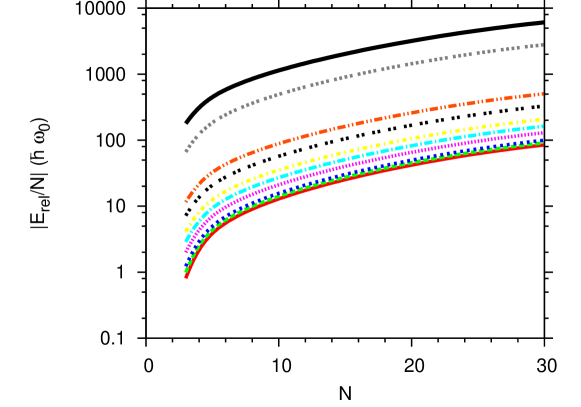
Figure 1: Relative energies per particle at several different values of the 3D scattering length as a function of particle number. The different values of the ratio are, from bottom to top: $a/\ell=100,10,5,2,4/3,1,2/3,1/2,1/5,$ and $1/10$.

The dependence on particle number $N$ is very explicit, but still two or rather three terms compete with their different $N$-scaling. We first show the relative energy per particle (i.e., the energy of the relative motion of the particles without the center-of-mass contribution corresponding to one particle moving in the external field) in figure 1 as function of $N$ for three dimensions. It happens that a two-body system is “unbound” in the oscillator model corresponding to positive relative energy. This occurs when the positive contribution in (46) is larger than the negative $V_{\textrm{shift}}$. However, $V_{\textrm{shift}}$ must dominate as $N$ increases, and in fact we find that once another particle is added, the relative energy is less than zero for any of the studied scattering lengths. The $N$-dependence is very smooth and steadily increases the binding which varies strongly when the scattering length approaches zero in units of the trap length. This is also the region where the magnitude of the two-body bound state energy increases rapidly.

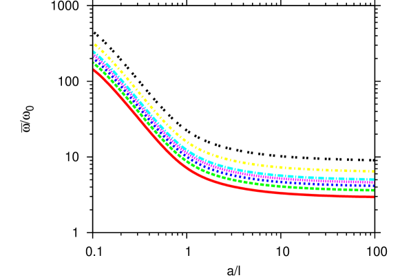
Figure 2: Degenerate frequency, $\bar{\omega}$ of the $N$-particle systems in 3D plotted logarithmically as a function of the ratio of the scattering length to the external confinement length. The different values of $N$ plotted are, from bottom to top: 3, 4, 5, 6, 10, 20, and 30.

The frequency dependent term in the energy proportional to $\hbar\bar{\omega}_{x}$ is simply the zero point motion of an oscillator. It is therefore also the smallest unit of excitation of the system corresponding to one particle lifted in one dimension from the ground to first excited state. This is the energy of the normal mode of excitation. The dependence is shown in figure 2 as function of scattering length from the Busch et al. model in (41). The frequency is small and constant for scattering lengths larger than the trap length, while it begins to grow very quickly as soon as the trap length exceeds the scattering length.

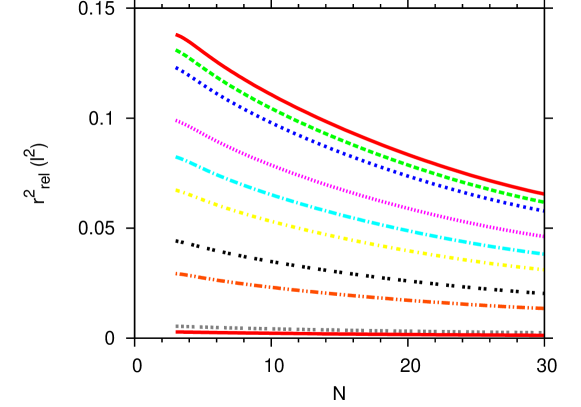
Figure 3: Relative sizes, $(r-R_{cm})^{2}$, at several different values of the 3D scattering length as a function of particle number. From top to bottom, the ratios are $a/\ell=100,10,5,2,4/3,1,2/3,1/2,1/5,$ and $1/10$.

The size of the system is, along with the energy, the most fundamental property. The intuitive implication that smaller radii follow larger binding is also observed in figure 3, regardless of the size of the scattering length, though at the weaker interactions the change is rather flat for the first few added particles. The $N$-dependence is again rather simple as seen in (52) where the mean square radius decrease with $1/\sqrt{N}$ for large $N$. Otherwise the radii are varying with frequency as usual. The interesting part is rather that the sizes increase substantially with scattering length for given particle number.

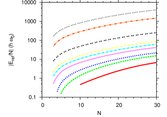
Figure 4: Relative energies per particle at several different values of the 2D scattering length as a function of particle number. From bottom to top, the ratios are $a/\ell=100,10,5,2,4/3,1,1/2,1/5,$ and $1/10$. Note that a few of the bottom lines at large scattering length over trap length ratios appear to stop at small particle numbers. This is because there is a sign change in the energy, which is discussed around (53).

We now repeat the procedure in two dimensions. The major difference is obviously from the adjusted oscillator input parameters. The energy and radius expressions are already given in (49) and (52). The $N$-dependence of the energy is shown in figure 4 where the same overall structure as in figure 1 appear. As in 3D, the energy decreases monotonically with the addition of more atoms for all scattering lengths.

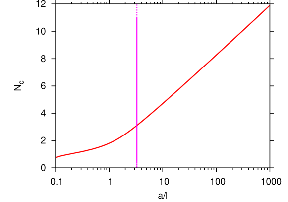
Figure 5: The critical number $N_{c}$ for 2D as function of the ratio of the scattering length to the external length. The vertical line is $a/\ell=3.3$, at which point (to the left of this line) all systems of more than two particles become self-bound.

The two-body energy shift is less negative because the size requirement to determine the frequency better matches the one-body frequency. Then several of the $N$-body energies are positive, although “binding” (negative energy) finally occurs by adding a sufficient number of particles. This critical number, $N_{c}$, where the system becomes self bound is given by

$$N_{c}=\frac{(\hbar\omega)^{2}}{V^{2}}\left[1+\sqrt{1+4\frac{\omega_{0}^{2}}{\omega^{2}}\left(\frac{V}{\hbar\omega}\right)^{2}}\right]\;,$$ (53)

which for the two dimensional case depends strongly on the initial scattering length as seen in figure 5. For the largest scattering length in figure 5 $N_{c}$ is about $12$, whereas there is binding for all particles for scattering lengths smaller than about three. As the scattering length becomes arbitrarily large, the critical number also increases, meaning that the addition of any number of particles is not sufficient to bind the system at infinite scattering length.

In figure 6 we show how the degenerate frequency for ten particle behaves as a function of the scattering length. The behaviour is very similar to then 3D result, with both curves turning up strong after the scattering length becomes less than the external confinement length.

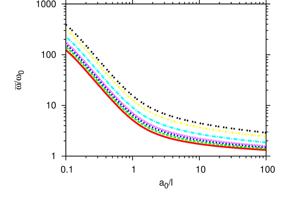
Figure 6: Degenerate frequencies, $\bar{\omega}$, of the $N$-particle systems in 2D plotted logarithmically as a function of the ratio of the scattering length to the external confinement length. The particle numbers plotted are, from bottom to top, 3, 4, 5, 6, 10, 20, and 30.

Figure 7 shows the size results in two dimensions. These also follow a slightly different trend than in three dimensions. In two dimensions, for several scattering lengths, the size actually increases for the addition of a particle (going from three to four particles), before falling for all additional particles. The scattering lengths where this behaviour is seen correspond roughly to those that have positive three-body energies. For smaller scattering lengths, the relative sizes decreases monotonically with an increase in particle number.

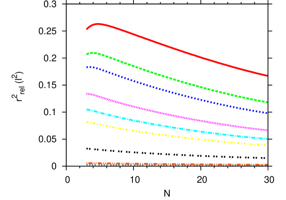
Figure 7: Relative sizes at several different values of the 2D scattering length as a function of particle number. From top to bottom, the ratios plotted are $a/\ell=100,10,5,2,4/3,1,1/2,1/5,1/10.$

3.4 One-body density

The one-body density matrix has information about the mean-field content of the wave function [20]. This is quantified by the eigenvalue in (38), which directly measures how much this state has the structure of a coherent (condensed) state. In figure 8, we see how this eigenvalue, $\lambda$, evolves for 3D with interaction strength and particle number. For the most part it increases with particle number, though at weaker interactions there is a small minimum around five or six particles and it increases thereafter, while it decreases uniformly with interaction strength.

The overall increase with $N$ is in agreement with the theorem that the mean-field wave function is approached as $N$ tends to infinity [20]. The condensate fraction is large for large scattering lengths where the external field is decisive, and consequently favors the corresponding mean-field structure. This follows from the fact noted above that the two-body wave functions become essentially non-interacting oscillator states given by the confinement ($\omega$ becomes small). On the other hand, for small scattering lengths the structure is far from that of a condensate. The particles are much more tightly bound with strong correlations. Again this is consistent with the fact that we have very strongly bound two-body states in this limit that are very different from the non-interacting harmonic states.

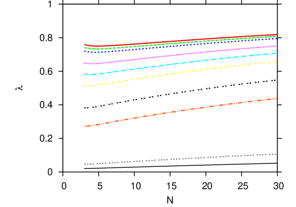
Figure 8: The value of $\lambda$ at several different values of the 3D scattering length as a function of particle number. From top to bottom, the ratios plotted are: $a/\ell=100,10,5,2,4/3,1,2/3,1/2,1/5,1/10.$

The question of whether a true condensate actually exists in a realistic quasi-2D setup with harmonic trapping potentials below a certain critical temperature [53, 3] will not be addressed here. We simply take the appearance of a large eigenvalue in the one-body density matrix as our working definition of a condensate as in the 3D case above. The condensate fraction are shown in figure 9 for the 2D system. The same tendency of increase with $N$ is present here. Again the condensate fraction is large (small) for large (small) scattering lengths compared to the size of the external field. This reflects the amount of correlation in the wave function precisely as for 3D. Quantitatively we find that $\lambda$ is even flatter as a function of particle number than in 3D, and it is also consistently higher for the same scattering length. We note that the 2D results consistently produce larger condensate fractions than in 3D. As we discuss below this is connected with the fact that the 2D case resembles a non-interacting system when $a\rightarrow\infty$ better than the 3D case does. The remaining deviation of $\lambda$ from unity is due to the separation of center-of-mass.

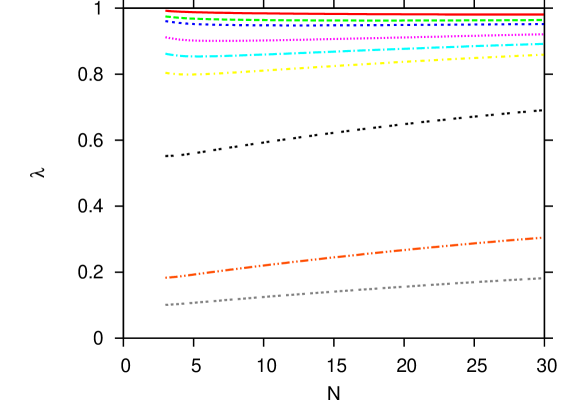
Figure 9: Condensate fraction at several different values of the 2D scattering length as a function of particle number. From top to bottom, the ratios plotted are: $a/\ell=100,10,5,2,4/3,1,1/2,1/5,1/10.$

3.5 Normal modes and symmetries

The characteristic properties of a system are reflected in the structures and energies of the normal modes. Here we discuss the energies of the degenerate frequencies which is the amount of energy required to excited the modes. Unfortunately, the degeneracy is itself an obstacle for understanding the uncoupled structures of single excitations. The reason is that any wave function expressed as a linear combination of the same energies is equally well qualified. The set of normal modes only has to be orthogonal, but that can be achieved in infinitely many ways. One general exception is if other conserved quantum numbers have to be restored by specific linear combinations of the degenerate states. Angular momentum is a prominent example in the absence of external fields.

We now discuss what determines the degeneracy, or equivalently what would break it. First, if all masses, all two-body interaction frequencies, and all one-body frequencies are equal, then $N-1$ degenerate frequencies are produced along with the one-body frequency, which is returned unchanged. If masses are changed, then the degeneracies are broken, and if $N-2$ masses are changed then all degeneracies will be broken. This is the same for the one-body frequencies (those in (2.1)), if $N-2$ of them are different from each other, then all the output frequencies will be different.

For the interaction frequencies in (2.1) the situation is slightly more complex. If one row and column in the $A$-matrix of (6) have the same interaction frequency, i.e., if this particle interacts the same with all other particles, then there will be at least one pair of degenerate frequencies. In general, of the $N(N-1)/2$ interaction frequencies (off-diagonal elements of the $A$-matrix), if $(N-1)(N-4)/2$ ($N>4$) of them are different, then that is enough to guarantee all symmetries are destroyed. However, all degeneracies can be broken with a wiser distribution of the different frequencies. If, for example, the frequencies immediately above the main diagonal of $A$ are all different and all the remaining ones being the same (a total of $N$ different off-diagonal frequencies), then that is enough to destroy all degeneracies of the resulting normal modes.

Thus, degeneracy can be broken or reached through many different paths. The structure of the resulting degenerate normal modes depends on the chosen path. We still find it interesting to investigate specially selected normal modes. If all particles are distinguishable it should in principle be possible to observe corresponding vibrational structures where each particle is detected. To probe the underlying structure, revealed by the normal modes, we therefore approach the degenerate limit from an entirely non-degenerate system. The two simplest ways are to differentiate the particles by minute differences in mass, or alternatively in one-body frequency.

We first notice that the normal modes are the results of transforming the set of oscillators to diagonal form. The energies and eigenvalues are obtained from the matrix depending on masses, external field frequency, and two-body interaction frequency. Thus by choosing all these parameters to be identical the normal modes in two and three dimensions are the same. This is achieved by the same masses, same external field, and corresponding choices of scattering lengths in 2D and 3D such that the two-body interaction frequencies from (48) are identical. The correspondence is seen in figure 10 where both scattering lengths are small at the same time and also increase simultaneously. The $2D$ scattering length approach an upper limit of about $1.14\ell_{2D}$ for increasing $a_{3D}$. The size in $2D$ is much smaller than in $3D$. In figure 10 we also show the relation between 2D and 3D oscillator shifts obtained from (46) for corresponding scattering lengths.

It is clear from the figure that it is possible to map 3D results onto 2D results, but the reverse is not always true. This is due to the different behaviour of the systems for large scattering length, where the energy and square radius of the two-body system are controlled by the properties of the external trap. In two dimensions we find that $\langle r^{2}\rangle=\ell^{2}$ when $a\rightarrow\infty$ and (45) then tells us that we have to choose $\omega=0$, i.e. we have a non-interacting system. For three dimensions, the situation is somewhat different as the virial theorem applied for $a\rightarrow\infty$, tells us that $\langle r^{2}\rangle=\ell^{2}/2$. From (45) we deduce that $\omega=2\sqrt{2}\omega_{0}$, i.e. our harmonic equivalent is an interacting system still. This also implies that the interaction frequency in 3D, $\omega$ in (48), can never be smaller than $2\sqrt{2}\omega_{0}$. In 2D, there is no lower limit for the interaction frequency and it eventually vanishes at a large enough scattering length where the external field determines all properties.

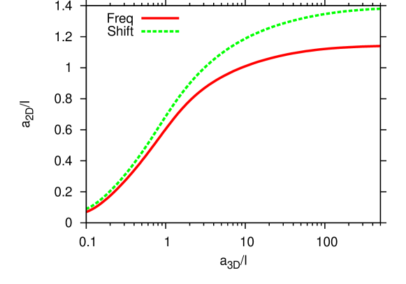
Figure 10: The relation between the 2D scattering length to external length ratio to the same quantity in 3D for both the interaction frequency (red curve) and energy shift (green curve).

From figure 10 we can in principle from a series of 2D calculations for different scattering lengths extract 3D results. The procedure is to start with the desired 3D scattering length, find the corresponding 2D scattering length, read off the related 2D results for normal modes, radii, and oscillator energy shift. The normal modes and radii are now the 3D results, and the 3D energy is obtained by finding the related 3D oscillator energy shift from figure 10 combined with the expression in (49). The procedure can be reversed provided the desired 2D scattering length is within the range accessible to conversion from 3D (i.e., $a_{2D}/\ell_{2D}\leq 1.14$).

The hamiltonian we obtain in our oscillator approximation can be decoupled by a change of coordinates as discussed above. The normal modes can therefore be viewed in one dimension at a time as the amplitudes with which each of the individual particles are moved when the corresponding mode is excited on top of the ground state. More explicitly, consider exciting the $i$’th mode with probability $p$, so that the wavefunction of the system becomes $|\Psi(t)\rangle=\sqrt{1-p^{2}}|0\rangle+\sqrt{p}e^{-i\bar{\omega}_{i}t}|i\rangle$, where $\bar{\omega}_{i}$ is the frequency of mode $i$. The displacement in time is then $x_{i}(t)=\langle\Psi(t)|x|\Psi(t)\rangle=A_{0i}\cos(\bar{\omega}_{i}t)$, with amplitude given by $A_{0i}=2\sqrt{p(1-p^{2})}\langle 0|x|i\rangle$. We illustrate the modes pictorially below. The fact that the different spatial directions are decoupled also implies that a spherical external field produces degenerate modes. This degeneracy can be lifted by deforming the field but such a symmetry breaking would only reflect the properties of the field. We therefore consider the one-dimensional eigenmodes which apply for both $2D$ and $3D$ when using a correspondence of scattering lengths down to $1D$ as was done between $2D$ and $3D$ in figure 10.

In figure 11 and figure 12 we show a sequence of modes for six and eight particles respectively. The dependence on scattering length is rather weak for both small and large $a/l$. The general picture that emerges from breaking the symmetry by mass differences is first that the energy of the center-of-mass oscillation is maintained. Second, the energies of the smallest and the largest mode correspond to oscillation where either the lightest or the heaviest particles move in one direction while all the others move less and in the opposite direction. The remaining modes with intermediate energies correspond to one particle joining the lone particle, moving in the order of increasing mass for each mode, though in most cases it appears that only one or two particles are displaced significantly, while the remainder stay in a slightly displaced clump. It should be noted that the normal modes are highly sensitive to the symmetries of the interaction, and how we broke the symmetry in order to show non-degenerate normal modes. In this present case, we changed the masses slightly to make the particles distinguishable, but still with identical interactions between all particles. We expect that if the interactions are changed slightly in a certain prescribed manner, then the normal modes will reflect the symmetries of that change.

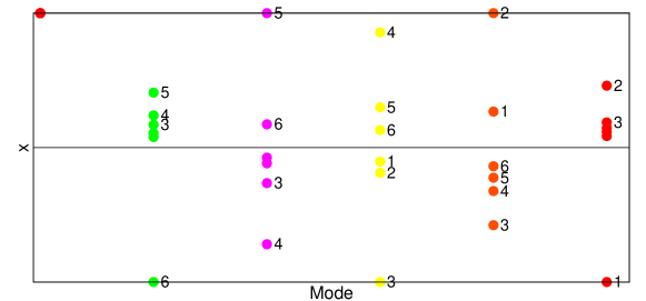
Figure 11: Amplitudes of the normal modes in the $x$ direction of a six particle system in 3D calculated with $a/\ell=1$, which is equivalent to a ratio of $0.61$ in the 2D. The largest amplitude is rescaled to unit magnitude. Points in the diagram are numbered from one to six with the mass increasing from particles one to six. Overlapping points are not labeled, and appear in groups usually close to the origin, which is indicate by the black solid horizontal line. The points oscillate through the equilibrium position (the black solid line) with a frequency of the given normal mode(e.g., $x_{i}(t)=A_{0i}\cos(\bar{\omega}_{i}t)$, where $A_{0i}$ are the amplitudes shown in the figure). The frequencies from left to right are 1.003, 10.433, 10.447, 10.456, 10.470, and 10.487 in units of $\omega_{0}$ and are not plotted to scale. The center of mass mode is the first mode shown.

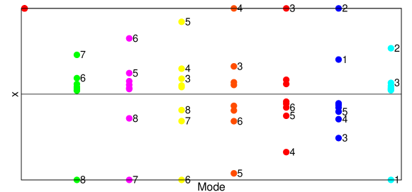
Figure 12: Amplitudes of the modes in the $x$ direction of an eight particle system in 3D with $a/\ell=1$, which has an equivalent ratio in 2D of 0.61. As in figure 11, the largest amplitude is normalized to one unit of length. Points in the diagram are numbered from one to eight with the mass increasing from particles one to eight (overlapping points are not labeled). These points oscillate through the equilibrium position, indicated by the solid black horizontal line, with a frequency of the given normal mode. The frequencies of the normal modes are, from left to right: 1.004, 12.030, 12.040, 12.050, 12.059, 12.069, 12.085, 12.097 in units of $\omega_{0}$ and are not plotted to scale. The center of mass mode is the first mode shown.

4 Summary and Conclusion

The properties of the quantum mechanical $N$-body system are determined from the basic one- and two-body interactions. However, in general this problem is very hard or impossible to solve. Here we use an approximate approach which replaces the interactions with quadratic forms in the coordinates, either by direct fits of the potentials or by adjusting parameters to reproduce crucial properties. This approximation allows analytical investigations of the $N$-body system with the properties expressed in terms of the two-body characteristics. Having such a direct approach to the general many-body problem can provide both important analytical insight and be a valuable benchmark for more intricate methods.

The most general harmonic oscillator potentials to describe one- and two-body interactions allow analytical solutions of the $N$-body Schrödinger equation. However, the center-of-mass degree of freedom requires special attention as we have described above. We have employed Cartesian coordinates and one-, two-, and three-dimensional systems are therefore equally simple to handle. We have discussed the properties of the resulting set of decoupled oscillators and their relation to the initial interactions. More explicitly we calculated energies, radii, and the one-body density matrix and presented its spectrum.

As an application of our formalism, we consider first the simplest case of $N$ bosons in a trap interacting through contact potentials. This was done by using a mapping from the energies and radii for the two-body system to the oscillator parameters for the analytical calculations. We note that while our choice of energy and radius as the essential parameters to reproduce in the two-body system was perhaps the most physically reasonable one, other choices are also possible as long as one has two quantities that fix the oscillator frequency and the shift. We calculated energies and radii as function of boson number and the scattering length as a measure of the interaction strength. Typically the binding energies increase and the radii decrease with $N$. We also discussed characteristic limits for scattering lengths much smaller and much larger than the length scale of the external trap.

An interesting calculation was done for the one-body density matrix for which we calculated the dependence of the lowest eigenvalue with the number of bosons and the scattering length, with a careful treatment removing the center-of-mass degree of freedom. The limits of large scattering length gave large condensate fractions, whereas for small scattering length we found a fragmented state. The former is due to the near non-interacting system, whereas the latter is caused by the strongly bound molecular state which introduces substantial amounts of correlations in the system. These conclusions apply equally for both two and three dimensions. We also computed the critical number of particles that can form a self bound system of negative energy. This number increases with increasing scattering length. In three dimensions this happens already for a few particles while in two dimensions more than 50 bosons are needed for large scattering lengths.

As a novelty, we considered the normal modes which are characteristic properties of any system. However, in the case of the $N$-boson system, there is a large degree of degeneracy that can obscure the detailed behaviour. The ambiguity due to degenerate eigenmodes is circumvented by breaking the symmetry and then approaching the limit of full degeneracy for the identical boson system. A different way of breaking the symmetry is to deform the external field but the resulting eigenmodes then reflect precisely the chosen deviation from spherical symmetry. We then computed the one-dimensional oscillatory eigenmodes which can be related to equivalent values of the scattering lengths in two and three dimensions. What we found in the normal modes was an interesting tendency for the particles to cluster in smaller groups and then perform motion with respect to other such groups. This implies that excitations can induce strong correlations in a many-boson system even when all interactions are equal.

The method that we have presented in this report is completely general and can be applied to systems in external fields or to self-bound structures. The treatment of deformation of the trap or the two-body interaction is straightforward and we expect that rotation of the external trapping potential poses no problem as well. While we have only treated bosons in this work, the extension to fermions is achieved through proper (anti-) symmetrization of the wave function and also Bose-Fermi mixtures are accessible. With the possibility of having displaced centers we can also apply the method for split traps, and also even more exotic geometries with mixed dimensions which are under current study within Fermi-Fermi mixtures of ultracold atoms [54, 55, 56, 57]. Our method can also be applied to cold polar molecules, in particular to the case where two-dimensional confinement is induced to make layered systems [58] where non-trivial two- and three-body bound states appear in the bilayer [59, 60, 61, 62, 63, 64] that open for study of various exotic many-body states in both bilayer and multi-layer systems [65, 66, 67, 68, 69, 70]. The form of the dipolar potential has harmonic oscillator shape in the inner part when particles are confined in multi-layers and we therefore expect the the method presented here to readily provide analytical results valid for intermediate and strong dipolar strength. The fact that normal modes are easily accessible with the harmonic method presented makes this even more interesting. This can help understand the modes of excitation in chains and complexes for use in thermodynamic calculations of system properties.

In conclusion, the analytic solutions of coupled harmonic oscillators can be used to study the overall properties of $N$-body systems and structures can be calculated in general from two-body properties for different particle number and geometries. This can serve as a valuable complement to the understand of results obtained with more intricate methods or help solve systems that are intractable in other approaches.

References

References

- [1] Goeppert-Mayer M and Jensen J H D 1955 Elementary Theory of Nuclear Shell Structure (John Wiley & Sons, Inc., New York)
- [2] Heyde K L G 1990 The Nuclear Shell Model (Springer, Berlin)
- [3] Bloch I, Dalibard J and Zwerger W 2008 Rev. Mod. Phys.80 885
- [4] Lizana L, Ambjörnsson T, Taloni A, Barkai E and Lomholt M A 2010 Phys. Rev. E 81 051118
- [5] Zhang J Y, Mitroy J and Varga K 2008 Phys. Rev. A 78 042705
- [6] Brosens F, Devreese J T and Lemmens L F 1997 Phys. Rev. E 55 227
- [7] Brosens F, Devreese J T and Lemmens L F 1997 Phys. Rev. E 55 6795
- [8] Brosens F, Devreese J T and Lemmens L F 1997 Phys. Rev. A 55 2453
- [9] Brosens F, Devreese J T and Lemmens L F 1998 Phys. Rev. E 57 3871
- [10] Brosens F, Devreese J T and Lemmens L F 1998 Phys. Rev. E 58 1634
- [11] Tempere J, Brosens F, Lemmens L F and Devreese J T 1998 Phys. Rev. A 58 3180
- [12] Lemmens L F, Brosens F and Devreese J T 1999 Phys. Rev. A 59 3112
- [13] Foulon S, Brosens F, Devreese J T and Lemmens L F 1999 Phys. Rev. E 59 3911
- [14] Tempere J, Brosens F, Lemmens L F and Devreese J T 2000 Phys. Rev. A 61 043605
- [15] Załuska-Kotur M A, Gajda M, Orłowski A and Mostowski J 2000 Phys. Rev. A 61 033613
- [16] Yan J 2003 J. Stat. Phys. 113 623
- [17] Gajda M 2006 Phys. Rev. A 73 023603
- [18] Busch T, Englert B G, Rzażewski K and Wilkens M 1998 Found. Phys. 28 548
- [19] Stöferle T, Moritz H, Günter K, Köhl M and Esslinger T 2006 Phys. Rev. Lett.96 030401
- [20] Yang C N 1962 Rev. Mod. Phys.34 694
- [21] Zinner N T and Jensen A S 2008 Phys. Rev. C 78 041306(R)
- [22] Pethick C J and L. P. Pitaevskii L P 2000 Phys. Rev. A 62 033609
- [23] Gajda M, Załuska-Kotur M A and Mostowski J 2000 J. Phys. B: At. Mol. Opt. Phys.33 4003
- [24] Gattobigio M, Kievsky A, Viviani M and Barletta P. 2009 Phys. Rev. A 79 032513
- [25] Stetcu I, Barrett B R, van Kolck U and Vary J P 2007 Phys. Rev. A 76 063613
- [26] Alhassid Y, Bertsch G F and Fang L 2008 Phys. Rev. Lett.100 230401
- [27] Rotureau J, Stetcu I, Barrett B R, Birse M C and van Kolck U 2010 Phys. Rev. A 82 032711
- [28] Stetcu I, Rotureau J, Barrett B R and van Kolck U 2010 Ann. Phys. 325 1644
- [29] Zinner N T, Mølmer K, Özen C, Dean D J and Langanke K 2009 Phys. Rev. A 80 013613
- [30] Özen C and Zinner N T 2009 Preprint arXiv:0902.4725v1
- [31] Carlson J, Chang S Y, Pandharipande V R and Schmidt K E 2003 Phys. Rev. Lett.91 050401
- [32] Chang S Y and Bertsch G F 2007 Phys. Rev. A 76 021603(R)
- [33] Gezerlis A and Carlson J 2008 Phys. Rev. C 77 032801(R)
- [34] Sørensen O, Fedorov D V and Jensen A S 2002 Phys. Rev. Lett.89 173002
- [35] Sørensen O, Fedorov D V and Jensen A S 2003 Phys. Rev. A 68 063618
- [36] Sørensen O, Fedorov D V and Jensen A S 2004 Phys. Rev. A 70 013610
- [37] Hanna G J and Blume D 2006 Phys. Rev. A 74 063604
- [38] Thøgersen M, Fedorov D V and Jensen A S 2007 Europhysics Letters 79 40002
- [39] Lim T K, Nakaichi S, Akaishi Y and Tanaka H 1980 Phys. Rev. A 22 28
- [40] Guangze H, Sørensen O, Jensen A S and Fedorov D V 2004 Phys. Rev. A 70 013609
- [41] Blume D 2005 Phys. Rev. B 72 094510
- [42] Christensson J, Forssén C, Åberg S and Reimann S M 2009 Phys. Rev. A 79 012707
- [43] Rontani M, Armstrong J R, Yu Y, Åberg S and Reimann S M 2009 Phys. Rev. Lett.102 060401
- [44] Liu X J, Hu H and Drummond P D 2010 Phys. Rev. B 82 054524
- [45] Rontani M, Åberg S and Reimann S M 2008 Preprint arXiv:0810.4305v1
- [46] Bertelsen J F and Mølmer K 2006 Phys. Rev. A 73 013811
- [47] Bertelsen J F and Mølmer K 2007 Phys. Rev. A 76 043615
- [48] Lovelace R V E and Tommila T J 1987 Phys. Rev. A 35 3597
- [49] Baym G and Pethick C J 1996 Phys. Rev. Lett.76 6
- [50] Fu H, Wang Y and Gao B 2003 Phys. Rev. A 67 053612
- [51] Zinner N T and Thøgersen M 2009 Phys. Rev. A 80, 023607
- [52] Thøgersen M, Zinner N T and Jensen A S 2009 Phys. Rev. A 80 043625
- [53] Bagnato V and Kleppner D 1991 Phys. Rev. A 44 7439
- [54] Nishida Y and Tan S 2008 Phys. Rev. Lett.101 170401
- [55] Nishida Y and Tan S 2009 Phys. Rev. A 79 060701(R)
- [56] Levinsen J, Tiecke T G, Walraven J T M and Petrov D S 2009 Phys. Rev. Lett.103 153202
- [57] Lamporesi G et al. 2010 Phys. Rev. Lett.104 153202
- [58] de Miranda M H G et al. 2011 Nature Phys. 7 502
- [59] Shih S M and Wang D W 2009 Phys. Rev. A 79 065603
- [60] Armstrong J R, Zinner N T, Fedorov D V and Jensen A S 2010 Europhysics Letters 91 16001
- [61] Klawunn M, Pivovski A and Santos L 2010 Phys. Rev. A 82 044701
- [62] Volosniev A, Zinner N T, Fedorov D V, Jensen A S and Wunsch B 2011 J. Phys. B 44 125301
- [63] Wunsch B et al. 2011 Phys. Rev. Lett.107 073201
- [64] Zinner N T et al. 2011 Phys. Rev. A 84 063606
- [65] Wang D W, Lukin M D and Demler E 2006 Phys. Rev. Lett.97 180413
- [66] Wang D W 2007 Phys. Rev. Lett.98 060403
- [67] Lutchyn R M, Rossi E and Das Sarma S 2010 Phys. Rev. A 82 061604(R)
- [68] Potter A C et al. 2010 Phys. Rev. Lett.105 220406
- [69] Pikovski A, Klawunn M, Shlyapnikov G V and Santos L 2010 Phys. Rev. Lett.105 215302
- [70] Zinner N T, Wunsch B, Pekker D and Wang D W 2012 Phys. Rev. A 85 013603