On the finite-dimensional marginals of shift-invariant measures

Abstract.

Let $\Sigma$ be a finite alphabet, $\Omega=\Sigma^{\mathbb{Z}^{d}}$ equipped with the shift action, and $\mathcal{I}$ the simplex of shift-invariant measures on $\Omega$. We study the relation between the restriction $\mathcal{I}_{n}$ of $\mathcal{I}$ to the finite cubes $\{-n,\ldots,n\}^{d}\subset\mathbb{Z}^{d}$, and the polytope of “locally invariant” measures $\mathcal{I}_{n}^{loc}$. We are especially interested in the geometry of the convex set $\mathcal{I}_{n}$ which turns out to be strikingly different when $d=1$ and when $d\geq 2$. A major role is played by shifts of finite type which are naturally identified with faces of $\mathcal{I}_{n}$, and uniquely ergodic shifts of finite type, whose unique invariant measure gives rise to extreme points of $\mathcal{I}_{n}$, although in dimension $d\geq 2$ there are also extreme points which arise in other ways. We show that $\mathcal{I}_{n}=\mathcal{I}_{n}^{loc}$ when $d=1$, but in higher dimension they differ for $n$ large enough. We also show that while in dimension one $\mathcal{I}_{n}$ are polytopes with rational extreme points, in higher dimensions every computable convex set occurs as a rational image of a face of $\mathcal{I}_{n}$ for all large enough $n$.

1. Introduction

Let $\Sigma$ be a finite alphabet, and let $\Omega=\Sigma^{\mathbb{Z}^{d}}$ denote the full $d$-dimensional shift over $\Omega$. $\Omega$ is compact and metrizable in the product topology, and the group $\mathbb{Z}^{d}$ acts continuously on $\Omega$ by translation. This action is denoted by $\Theta$ and the action of $u\in\mathbb{Z}^{d}$ by $\Theta^{u}$:

$$(\Theta^{u}x)_{v}=x_{u+v}.$$

The translation-invariant probability measures on $\Omega$ play an important role in dynamical systems theory, probability and thermodynamic formalism [14], but often these objects are subtle and difficult to describe. Therefore constructions of examples and fine analysis of lattice models in physics often proceed by studying appropriate measures on finite lattices which converge, as the lattices grow, to a measure on the full shift.

Thus it is natural to study the relation between the simplex of measures on finite lattices, and the restriction to the same lattices of the simplex of invariant measures on the full shift. Intermediate between them is a third object, namely, the polytope of measures which are “locally invariant”. In this paper we make some contributions to the understanding of these objects. We particularly focus on identifying their extreme points, both because these determine the geometry of the sets, and because in the set of invariant measures on the infinite lattice they correspond to the ergodic measures, which are the most dynamically significant; and it is reasonable to ask if there is a similar interpretation at the finite level. Some previous work dealing with the problem of building a process from a finite-dimensional marginal can be found in [10] and overlaps with our results in Theorem 3 and Theorem 9.

Let us introduce some notation. The space of Borel probability measures on $\Omega$ is denoted by $\mathcal{P}=\mathcal{P}(\Omega)$, and the subset of measures invariant under the action $\Theta$ is denoted $\mathcal{I}$. The space $\mathcal{P}$ (and hence $\mathcal{I}$) carries the weak-* topology when measures are identified with bounded linear functionals on $C(\Omega)$, and both spaces are closed and convex. The set $\mathcal{I}$ is in fact a simplex, that is, each point in it has a unique representation as the integral of a measure supported on its extreme points, and in fact the extreme points of $\mathcal{I}$ are precisely of the ergodic invariant measures. $\mathcal{I}$ also has the remarkable feature that its extreme points are dense. For proofs of these statements we refer to [4].

Let

$$\Lambda_{n}=\{-n,\ldots,n\}^{d}\subseteq\mathbb{Z}^{d}$$

and let

$$\Omega_{n}=\Sigma^{\Lambda_{n}}.$$

The finite-dimensional simplex of probability measures on $\Omega_{n}$ is denoted by $\mathcal{P}_{n}=\mathcal{P}(\Omega_{n})$. Let $\pi_{n}:\Omega\rightarrow\Omega_{n}$ denote the restriction operator $x\mapsto x|_{\Lambda_{n}}$, and also denote by $\pi_{n}$ the induced map $\mathcal{P}\rightarrow\mathcal{P}_{n}$. The image of $\mathcal{I}$ under this map is denoted $\mathcal{I}_{n}$. Since $\mathcal{I}$ is compact and convex, and since $\pi_{n}$ is continuous and linear, $\mathcal{I}_{n}$ is a closed convex subset of the finite-dimensional vector space $\mathcal{P}_{n}$.

Another space of interest is the space $\mathcal{I}_{n}^{loc}\subseteq\mathcal{P}_{n}$ of locally invariant measures. To define these, we define a pattern to be a partial configuration $a:E\rightarrow\Sigma$, for a finite set $E\subseteq\mathbb{Z}^{d}$. Translation $\Theta^{u}a$ of a pattern $a$ on $E$ is the pattern on $E-u$ defined by $(\Theta^{u}a)_{v}=a_{v+u}$. The cylinder set $[a]\subseteq\Omega$ associated to $a\in\Sigma^{E}$ is

$$[a]=\{x\in\Omega\,:\,x|_{E}=a\}$$

and when $E\subseteq\Lambda_{n}$ we denote

$$[a]_{n}=\{b\in\Omega_{n}\,:\,b|_{E}=a\}.$$

Note that $[\Theta^{u}a]_{n}$ is defined for $a:E\rightarrow\Sigma$ as long as $E-u\subseteq\Lambda_{n}$.

A measure $\mu\in\mathcal{P}$ is invariant under $\Theta$ if $\mu(\Theta^{u}[a])=\mu([a])$ for every $u\in\mathbb{Z}^{d}$ and every pattern $a$. Similarly, local invariance of $\mu\in\mathcal{P}_{n}$ means that for every $E\subseteq\Lambda_{n}$, for every $a\in\Sigma^{E}$, and for every $u\in\mathbb{Z}^{d}$ such that $E-u\subseteq\Lambda_{n}$, we have

(1.1) $$\mu([a]_{n})=\mu([\Theta^{u}a]_{n})$$

The set of locally invariant measures on $\Omega_{n}$ is denoted $\mathcal{I}_{n}^{loc}$. Clearly $\mathcal{I}_{n}\subseteq\mathcal{I}_{n}^{loc}\subseteq\mathcal{P}_{n}$, and each of these spaces is a closed, convex subset of the next.

Recall that a polytope is the convex hull of a finite set. The intersection of a polytope with an affine subspace is again a polytope. Note that as $E,a,n$ range over all their possible values, each of the conditions (1.1) amounts to intersecting $\mathcal{P}_{n}$ with a linear subspace. If we choose as a basis for $\mathcal{P}_{n}$ the probability measures which give mass to a single cylinder set $[a]_{n},$ $a\in\Omega_{n}$, then these subspaces are defined by linear equations with integer coefficients. It follows that:

Theorem 1.

$\mathcal{I}_{n}^{loc}$ is a polytope whose extreme points are measures with rational range, that is $\mu(A)\in\mathbb{Q}$ for all $A\subseteq\Omega_{n}$.

The last statement holds independent of the dimension. However, the nature of these extreme points differs quite drastically in dimension 1 and in higher dimensions.

Theorem 2.

For $d=1$, every extreme point of $\mathcal{I}_{n}^{loc}$ is the projection of the uniform measure on a $\Theta$-periodic orbit. In particular, $\mathcal{I}_{n}=\mathcal{I}_{n}^{loc}$.

Note however that $\mathcal{I}_{n}^{loc}$ is not a simplex, and measures may not have a unique decomposition as convex combinations of extreme points; thus in this sense the analogy of extreme points and ergodic measures is false. Here is a simple example demonstrating this. Consider the case $d=1$ and $n=1$, so we are considering measures on words of length $|\Lambda_{1}|=3$. Let $\Sigma=\{1,2,3,4\}$. Let $\mu\in\mathcal{P}_{3}$ be the uniform measure on sequences in which no symbol appears twice. Let $S_{3}$ and $S_{4}$ denote the sets of sequences of length $3$ and $4$, respectively, in which no symbol appears twice. To each $a\in S_{3}\cup S_{4}$ we can associate the $\Theta$-invariant measure $\mu_{a}\in\mathcal{I}$ supported on the orbit of the periodic point $\ldots aaa\ldots\in\Omega$. One may verify directly, or using Proposition 5 below, that $\pi\mu_{a}$ is an extreme point in $\mathcal{I}_{1}$. It is then clear that

$$\mu=\frac{1}{|S_{3}|}\sum_{a\in S_{3}}\mu_{a}=\frac{1}{|S_{4}|}\sum_{b\in S_{4}}\mu_{b}.$$

By replacing individual symbols by sequences of a fixed length which have the property that any subsequence of a concatenation of them has a unique parsing, we can construct, over a given alphabet, examples like this for any $n$.

In contrast to Theorem 2, in higher dimensions we have the following.

Theorem 3.

For $d\geq 2$ the map $\pi_{n}:\mathcal{I}\rightarrow\mathcal{I}_{n}^{loc}$ is not onto. In particular there are extreme points of $\mathcal{I}_{n}^{loc}$ which do not correspond to invariant measures.

The result was also proved by Pivato in [10] using a result of Robinson [13].

We may describe the relation between the sets $\mathcal{I}_{n}$ , $\mathcal{I}_{n}^{loc}$ and $\mathcal{I}$ is as follows. The restriction maps $\pi_{n}$ are compatible in the sense that, if $\widetilde{\pi}_{n+1,n}:\mathcal{I}_{n+1}\rightarrow\mathcal{I}_{n}$ is again given by restriction, $a\mapsto a|_{\Lambda_{n}}$, then

$$\pi_{n}=\widetilde{\pi}_{n+1,n}\pi_{n+1}.$$

Also, the projections $(\pi_{n}(\mu))_{n=1}^{\infty}$ completely determine $\mu\in\mathcal{P}$. Therefore $\mathcal{I}$ is the inverse limit of the sets $\mathcal{I}_{n}$, and hence, in dimension $1$, the inverse limit also of the $\mathcal{I}_{n}^{loc}$. However, for $d\geq 2$ the situation is more subtle, due to the fact that the maps $\pi_{n}$ are not onto $\mathcal{I}_{n}^{loc}$. Rather, we have that following. For $k>n$ let $\widetilde{\pi}_{k,n}:\mathcal{I}_{k}^{loc}\rightarrow\mathcal{I}_{n}^{loc}$ be defined by restriction, as above. Then it is an easy consequence of the definitions that

Proposition 4.

$\mathcal{I}_{n}=\bigcap_{k=n}^{\infty}\widetilde{\pi}_{k,n}(\mathcal{I}_{n}^{loc})$.

The new features of $\mathcal{I}_{n}$ which emerge in dimensions $d\geq 2$, as well as the tools used in their analysis, are closely related to the dynamics of multidimensional shifts of finite type. Recall that a closed, $\Theta$-invariant subset $X\subseteq\Omega$ is a shift of finite type (SFT) if there is an $n$ and a set of patterns $L\subseteq\Omega_{n}$ such that $x\in X$ if and only if no pattern from $L$ appears anywhere in $x$, that is, if $\pi_{n}(\Theta^{u}x)\notin L$ for every $u\in\mathbb{Z}^{d}$. In this case we write $X=SFT(L)$. Given an SFT $X$ (or more generally any closed, $\Theta$-invariant subset of $\Omega$) we denote by $\mathcal{I}(X)\subseteq\mathcal{I}$ the set of invariant measures supported on $X$. This is a closed convex set.

A face of a convex set $C$ in a real vector space is the intersection of the boundary $\partial C$ with a supporting affine subspace. If this subspace is defined over the rationals, the face is said to be rational. A face consisting of one point is an exreme point, and the set of extreme points of $C$ is denoted $\operatorname{ext}C$. The relation between SFTs and $\mathcal{I}_{n}$ is given by the following simple but fundamental proposition.

Proposition 5.

If $X$ is an SFT defined by $L\subseteq\Omega_{n}$ then the set $\pi_{n}(\mathcal{I}(X))$ is a rational face of $\mathcal{I}_{n}$. In particular, if $X$ is uniquely ergodic and $\mu$ is the unique invariant measure on $X$, then $\pi_{n}(\mu)\in\operatorname{ext}\mathcal{I}_{n}$.

Theorem 3 follows from Theorem 1, the proposition above, and the following:

Theorem 6.

For $d\geq 2$ there exist uniquely ergodic SFTs and two cylinder sets $C,C^{\prime}$ such that the unique invariant measure $\mu$ satisfies $\mu(C)/\mu(C^{\prime})\notin\mathbb{Q}$.

Alternatively there is an argument using undecidability of Wang’s tiling problem, see Section 4.

As a geometric consequence, if $X$ is an SFT as in the proposition it follows that, for large enough $n$, the projection of its unique invariant measure to $\mathcal{I}_{n}$ is located in the interior of a face of $\mathcal{I}_{n}^{loc}$, since the extreme points of the face containing the measure are rational.

We now turn to the structure of $\mathcal{I}_{n}$. While uniquely ergodic SFTs give rise to extreme points, these do not exhaust the possibilities:

Theorem 7.

For $d\geq 2$ there are extreme points of $\mathcal{I}_{n}$ which do not arise as restrictions of the unique invariant measure on a uniquely ergodic SFT.

Thus we do not have a complete desription of the extreme points. Nevertheless we can give some precise indication of the richness of the sets $\mathcal{I}_{n}$. For this we require two definitions.

We say that a convex set $A\subseteq\mathbb{R}^{n}$ is effective if there is an algorithm which, on input $k$, computes the extreme points of a rational polytope polytope $A_{k}$ which contains $A$, and such that $A=\bigcap_{k=1}^{\infty}A_{k}$. This class, while countable, is very broad, including e.g. all rational polytopes, the closed convex hulls of computable and bounded sequences of points, etc. A stronger condition is that of computability: $A$ is computable if there is an algorithm which produces, for each $n$, a convex polytope within Hausdorff distance $1/n$ of $A$. There are effective sets which are not computable.

We say that a convex set $B\subseteq\mathbb{R}^{m}$ is a rational image of a convex set $A\in\mathbb{R}^{n}$ if there is a rational matrix and associated linear map $T:\mathbb{R}^{n}\rightarrow\mathbb{R}^{m}$ such that $TA=B$.

Theorem 8.

Let $d\geq 2$. Then $A$ is an effective convex set if and only if for all large enough $n$, it is a rational image of a rational face of $\mathcal{I}_{n}$.

It is not hard to show that, for fixed $n$, the sets $\mathcal{I}_{n}$ are effective. On the other hand there exist effective non-computable convex sets, and rational images of computable sets are computable. Thus:

Theorem 9.

For $d\geq 2$ the sets $\mathcal{I}_{n}$ are effective but, for large enough $n$, they are not computable.

Non-computability of $\mathcal{I}_{n}$ was also established in [10].

These results should be compared with other propertis of multidimensional symbolic dynamics which have emerged recently, in which the range of certain dynamical parameters have been characterized in terms of the level of computability [7, 17, 6].

Let us summarize the main points above. Proposition 5 shows that shifts of finite type whose set of forbidden patterns is contained in $\Omega_{n}$ can naturally be identified with faces of $\mathcal{I}_{n}$. Moreover, for shifts of finite type carrying a unique invariant measure, the corresponding face reduces to a single point which is an extreme point of $\mathcal{I}_{n}$. This fact holds irrespective of the dimension $d$ of the lattice. For $d=1$ this accounts for all of the extreme points, which arise as projections of uniform measures on periodic orbits (Theorem 2). For $d\geq 2$ there still exist extreme points of $\mathcal{I}_{n}$ corresponding to projections of uniform measures on periodic orbits, but there are also many extreme points not of this kind. All these “strange” extreme points, as well as some of the extreme points arising from the invariant measures of uniquely ergodic SFTs, are properly contained in $\mathcal{I}_{n}^{loc}$, which is a rational polytope. As for the faces of $\mathcal{I}_{n}$ in dimension $d\geq 2$, we have characterized them up to rational images, but it remains an interesting open problem to better understand the faces themselves.

2. Proof of Theorem 1

In this section we prove Theorem 1, which holds in any dimension $d$.

Let $\mathcal{V}_{n}$ denote the space of real-valued functions $x:\Omega_{n}\rightarrow\mathbb{R}$, $a\mapsto x_{a}$. Each $x\in\mathcal{V}_{n}$ may also be identified with a signed measure, given by $x(A)=\sum_{a\in A}x_{a}$. With this identification, we have

$$\mathcal{P}_{n}=\{x\in\mathcal{V}_{n}\,:\,\sum x_{a}=1\mbox{ and }x_{a}\geq 0\mbox{ for all }a\in\Omega_{n}\}.$$

The extreme points are the vectors $\delta_{a}$ for $a\in\Omega_{n}$ and the faces of $\mathcal{P}_{n}$ are precisely the subspace of $\mathcal{V}_{n}$ determined by setting $x_{a}=0$ for some $A\subseteq\Omega_{n}$. Now, in order for $x\in\mathcal{P}_{n}$ to belong to $\mathcal{I}_{n}^{loc}$ it must additionally satisfy the condition in Equation (1.1) for each applicable choice of $E,u$ and $a\in\Sigma^{E}$, and this condition is nothing other than the equation

$$\sum_{b\in\Omega_{n}\,:\,b|_{E}=a}x_{b}=\sum_{c\in\Omega_{n}\,:\,(\Theta^{u}c)|_{E}=a}x_{c}$$

which is an integer-valued linear equation in $\{x_{b}\}_{b\in\Omega_{n}}$. Let $\mathcal{W}_{n}$ denote the solution set of these equations for all parameters $E,u,a$. Then $x$ is an extreme point of $\mathcal{I}_{n}^{loc}$ if and only if $\{x\}$ is the intersection of $\mathcal{W}_{n}$ with some face of $\mathcal{P}_{n}$. Such an intersection is a solution of a family of linear equations with integer coefficients. Such equations have rational solutions if they have solutions at all, so if there is a unique solution it must be rational. $\square$

Another consequence of this proof is the following:

Corollary 10.

With $\mathcal{W}_{n}$ as in the proof of Theorem 1, the faces of $\mathcal{I}_{n}^{loc}$ are precisely the intersections of $\mathcal{W}_{n}$ with faces of $\mathcal{P}_{n}$.

3. Proofs in dimension one

We first prove a more general fact: For $d=1$, every $\mu\in\mathcal{I}_{n}^{loc}$ is the image under the restriction map $\pi_{n}:\mathcal{I}\rightarrow\mathcal{I}_{n}$ of a stationary $(n-1)$-step Markov measure $\widetilde{\mu}\in\mathcal{I}$.

To see this we construct the chain explicitly. For $\mu\in\mathcal{I}_{n}^{loc}$ we first construct a Markov chain with state space

$$V=\{a\in\Sigma^{[-n;n-1]}\,:\,\mu([a]_{n})>0\}$$

and given $a\in V$ let

$$E_{a}=\{b\,:\,aa^{\prime}=b^{\prime}b\mbox{ for some }a^{\prime},b^{\prime}\in\Sigma\mbox{, and }\mu([aa^{\prime}]_{n})>0\}$$

(here $aa^{\prime}\in\Sigma^{[-n;n]}$ is the concatenation of $a$ and $a^{\prime}$. Note that $aa^{\prime}\in\Omega_{n}$). Define the stochastic matrix $(p_{a,b})_{a,b\in V}$ by

$$p_{a,b}=\frac{\mu([aa^{\prime}]_{n})}{\sum_{a^{\prime\prime}\in\Sigma}\mu([aa^{\prime\prime}]_{n})}$$

whenever $b\in E_{a}$ and $aa^{\prime}=b^{\prime}b$ for $a^{\prime},b^{\prime}\in\Sigma$ (note that $a^{\prime},b^{\prime}$ are determined uniquely), and set $p_{a,b}=0$ otherwise.

It is now straightforward to verify that the the probability vector $p(a)=\mu([a]_{n})$, $a\in V$, is stationary for the stochastic matrix $(p_{a,b})_{a,b\in V}$. By construction the shift-invariant measure $\widetilde{\mu}$ on $V^{\mathbb{Z}}$, corresponding to this Markov chain, may be identified with an invariant measure $\widetilde{\mu}$ on $\Sigma^{\mathbb{Z}}$ via the factor map $\tau:V^{\mathbb{Z}}\rightarrow\Sigma^{\mathbb{Z}}$ given by

$$\tau(x)_{n}=(x_{n})_{0}.$$

One verifies that the latter measure has marginal equal to $\mu$. $\square$

Let us make a few comments on this construction. First, the measure $\widetilde{\mu}$ by construction gives positive measure to $[a]\subseteq\Sigma^{\mathbb{Z}}$ for $a\in V$, and hence the matrix $(p_{a,b})$ is irreducible. Second, the transition graph $G=(V,E)$, defined with $V$ as above and $E=\{(a,b)\;:\;a\in V\,,\,b\in E_{a}\}$, is determined completely by the support of $\mu$. If $\nu\in\mathcal{I}_{n}^{loc}$ is a measure with $\operatorname{supp}\nu\subseteq\operatorname{supp}\mu$, then the graph constructed as above for $\nu$ will be a sub-graph of the one constructed for $\mu$. Consequently, $\widetilde{\nu}$ is supported on $\operatorname{supp}\widetilde{\mu}$, although its support may actually be smaller. In particular this holds whenever $\nu$ is the marginal on $\Omega_{n}$ of an invariant measure on $\operatorname{supp}\widetilde{\mu}$.

Proof of Theorem 2.

Let $\mu\in\mathcal{I}_{m}^{loc}$ be an extreme point. By the argument above it is the image of an invariant Markov measure $\widetilde{\mu}$. Also, since $\mu$ is an extreme point and $\mathcal{I}_{n}^{loc}=\mathcal{W}_{n}\cap\mathcal{P}_{n}$, there is a face $\mathcal{F}$ of $\mathcal{P}_{n}$ such that $\mathcal{W}_{n}\cap\mathcal{F}=\{\mu\}$. Here $\mathcal{W}_{n}\subseteq\mathcal{V}_{n}$ is the subspace defined by the local invariance conditions as in the proof of Theorem 1. We claim that $\mu$ must be the uniform measure on a periodic orbit, or, equivalently, that the transition graph $G=(V,E)$ of $\widetilde{\mu}$ constructed as above consists of a single cycle. Indeed, otherwise there would be a proper subgraph $G^{\prime}\subseteq G$ which is itself a directed cycle. Taking any positive stochastic matrix for $G^{\prime}$, the corresponding Markov measure projects down to a locally invariant measure $\nu\in\mathcal{I}_{n}^{loc}$. Since $\operatorname{supp}\nu\subseteq\operatorname{supp}\mu$ we have  $\nu\in\mathcal{F}$ (recall that faces in $\mathcal{P}_{n}$ are defined by setting some set of coordinates to zero), so $\nu\in\mathcal{W}_{n}\cap\mathcal{F}=\{\mu\}$. On the other hand, since $G^{\prime}$ is a proper subgraph of $G$ there is some $A\subseteq\Omega_{n}$ with $\nu(A)=0$ and $\mu(A)>0$, a contradiction. ∎

4. Proofs of higher dimensional results

We now turn to the higher dimensional case, $d\geq 2$. Let us first show that $\mathcal{I}_{n}^{loc}\neq\mathcal{I}_{n}$. We shall give two different proofs of this fact. We begin with one based on Berger’s theorem [2], which asserts that there is no algorithm which computes, for $L\subseteq\Omega_{n}$, whether $SFT(L)=\emptyset$.

First proof of Theorem 3.

Suppose that for every $n$ all of the extreme points of $\mathcal{I}_{n}^{loc}$ were projections of invariant measures. We show that we could then decide, given $L\subseteq\Omega_{n}$, whether $SFT(L)=\emptyset$, contradicting Berger’s theorem.

Suppose $L\subseteq\Omega_{n}$ is given and define the convex hull

$$\mathcal{F}=\operatorname{conv}\{\delta_{a}\,:\,a\in\Omega_{n}\setminus L\}.$$

This is a face of $\mathcal{P}_{n}$, and $\mathcal{F}\cap\mathcal{W}_{n}$ is a face of $\mathcal{I}_{n}^{loc}$, where $\mathcal{W}_{n}$ is the subspace defined by the local invariance conditions, as in the proof of Theorem 1. Since $\mathcal{W}_{n}$ is given explicitly by integer linear equations, and $L$ is a given finite set, we can decide if $\mathcal{F}\cap\mathcal{W}_{n}=\emptyset$. In order to complete the proof, it is enough to show that $\mathcal{F}\cap\mathcal{W}_{n}=\emptyset$ if and only if $SFT(L)=\emptyset$.

In one direction, if $SFT(L)\neq\emptyset$ then there is an invariant measure $\mu$ on $SFT(L)$, and by definition $\mu([a])=0$ for $a\in L$, so also

$$(\pi_{n}\mu)([a]_{n})=0.$$

Thus $\pi_{n}\mu\in\mathcal{F}\cap\mathcal{W}_{n}$, so $\mathcal{F}\cap\mathcal{W}_{n}\neq\emptyset$.

Conversely, If $\nu\in\mathcal{F}\cap\mathcal{W}_{n}$ then we can write $\nu=\sum p_{i}\nu_{i}$ where $p=(p_{i})$ is a probability vector and $\nu_{i}\in\operatorname{ext}\mathcal{I}_{n}^{loc}$. In fact, clearly $\nu_{i}\in\mathcal{F}\cap\mathcal{W}_{n}$ (this is true for geometric reasons, but, more concretely, because $\nu([a]_{n})=0$ for $a\in L$ and therefore, since $\nu=\sum p_{i}\nu_{i}$, also $\nu_{i}([a]_{n})=0$ for all $i$ and $a\in L$. This implies by definition that $\nu_{i}\in\mathcal{F}$). By assumption, $\nu_{i}=\pi_{n}\mu_{i}$ for some invariant measure $\mu_{i}$ on $\Omega$. But $\mu([a])=0$ for $a\in L$, so $\mu$ is supported on $SFT(L)$, and therefore $SFT(L)\neq\emptyset$. ∎

Evidently, one cannot decide whether a locally invariant measure on $\Omega_{n}$ can be extended to an invariant measure on $\Omega$. This is the analogue of the undecidability of the extension problem for SFTs, i.e. that one cannot decide, given a pattern $a\in\Sigma^{E}$, whether there is a point $x\in SFT(L)$ such that $x|_{E}=a$.

We now turn to $\mathcal{I}_{n}$. Since in dimension $1$ the sets $\mathcal{I}_{n}$ and $\mathcal{I}_{n}^{loc}$ coincide, Theorem 2 can be re-stated as follows: if $X\subseteq\Omega$ is a periodic orbit then the unique invariant measure on it projects to an extreme point of $\mathcal{I}_{n}$ for all large enough $n$. Here is the proof in the multi-dimensional case:

Proof of Proposition 5.

Suppose $L\subseteq\Omega_{k}$ and $X=SFT(L)\neq\emptyset$. For $n\geq k$ let $\mathcal{F}\subseteq\mathcal{P}_{n}$ be the face defined by the condition $\mu([a]_{n})=0$ for $a\in L$. Then, as in the proof of Theorem 3, any $\mu\in\mathcal{F}\cap\mathcal{I}_{n}$ is the projection under $\pi_{n}$ of a measure supported on $X$. Since $\mathcal{F}\cap\mathcal{I}_{n}$ is a face of $\mathcal{I}_{n}$, this proves the first part of the proposition. The second follows from the fact that when $X$ is uniquely ergodic there is only one measure in $\mathcal{I}$ supported on $X$ and therefore $\mathcal{F}\cap\mathcal{I}_{n}$ is a singleton (consisting of the projection of this measure to $\mathcal{I}_{n}$), and hence an extreme point. ∎

Alternatively, the following proof gives some additional geometric information:

Second proof of Theorem 3.

Assuming Theorem 6, there is an SFT $X=SFT(L)$ which projects to an extreme point of $\mathcal{I}_{n}$ for all large enough $n$, but for which there are disjoint clopen sets with masses whose ratio is irrational, and therefore by Theorem 1 cannot be an extreme point of $\mathcal{I}_{n}^{loc}$. ∎

We offer two proofs of Theorem 6.

First proof.

One can apply [7, Theorem 4.1]. This uses the fact that there are computable irrational numbers (e.g. there is an algorithm which given $n$ outputs the $n$-th binary digit of $\sqrt{2}$), and requires a few small modifications to the proof in [7, Theorem 4.1] in order to verify that the resulting SFT is uniquely ergodic, but these are straightforward given the machinery in [9]. ∎

Second proof.

The second proof relies on two facts. First, there are translation-minimal spaces of geometric tilings (i.e. tilings of the Euclidean plane by translates and rotations of finitely many polygons) in which the ratios of the areas of prototiles is irrational. An example of such a tiling is the Penrose kites-and-darts tiling system [11]. Second, there is an orbit equivalence between this system and the suspension of an appropriate uniquely ergodic $\mathbb{Z}^{2}$-SFT [15]. This gives appropriately weighted cylinder sets. More details are provided in Section 6. ∎

5. Rational images of $\mathcal{I}_{n}$

In this section we prove Theorems 7 and 8. We rely on some results about effective subdynamics of SFTs which appeared in [6] and were generalized in [1] and [3] (the earlier in [7] can easily be modified as well to give the same results). We describe these results next.

We begin with some definitions about one-dimensional patterns, which we call words. Below we shall use superscrips to indicate the dimensions of patterns and probability spaces on patterns. Thus $\Omega_{n}^{1}$ is the space of 1-dimensional patterns over $\Sigma$, with shape $\Lambda_{n}^{1}=[-n,n]\cap\mathbb{Z}$, and $\Omega_{n}^{2}$ is the space of two-dimensional patterns over $\Lambda_{n}^{2}=[-n,n]^{2}\cap\mathbb{Z}$. We similarly write $\mathcal{P}_{n}^{1}$ and $\mathcal{P}_{n}^{2}$ for the space of probability measures on $\Omega_{n}^{1},\Omega_{n}^{2}$, respectively.

The set of words over an alphabet $\Sigma_{0}$ is $\Sigma_{0}^{*}=\bigcup_{n=0}^{\infty}\Sigma_{0}^{n}$ . Consider an alphabet $\Sigma_{0}$ and a family $L\subseteq\Sigma^{*}$. The subshift $X\subseteq\Sigma^{\mathbb{Z}}$ consisting of all sequences which omit the patterns from $L$ is a subshift which we shall say is of infinite type and denote $SIT(L)$. If we write $L_{n}=L\cap\bigcup_{i=1}^{n}\Omega_{n}$ then $SIT(L)$ is equal to

$$SIT(L)=\bigcap_{n=1}^{\infty}SFT(L_{n}).$$

Note that in fact every subshift arises in this way.

A subshift $X$ is effective if there is a recursively enumerable set $L$ such that $X=SIT(L)$; that is, $L$ should have the property that there exists an enumeration $L=\{a_{1},a_{2},\ldots\}$ and an algorithm which on input $n$ outputs $a_{n}$.

Effective subshifts form a much larger class than SFTs, but there is a close relation. Given $X\subseteq\Sigma^{\mathbb{Z}}$ let $\widehat{X}\subseteq\Sigma^{\mathbb{Z}^{2}}$ denote the subshift

$$\widehat{X}=\{\widehat{x}\in\Sigma^{\mathbb{Z}^{2}}\,:\,\widehat{x}|_{\mathbb{Z}\times\{0\}}\in X\mbox{ and }\widehat{x}_{i,j}=\widehat{x}_{i,j+1}\mbox{ for all }i,j\in\mathbb{N}\}$$

that is, $\widehat{X}$ is obtained from $X$ be extending each configuration $x\in X$ vertically to a 2-dimensional configuration in which one sees $x_{i}$ in the $i$-th column.

Theorem 11 ([6, 3, 1]).

If $X\subseteq\Sigma^{\mathbb{Z}}$ is an effective subshift then there is a 2-dimensional SFT $Y$ which factors onto $\widehat{X}$. Furthermore $Y$ can be chosen so that it has entropy $0$ and has no periodic points.

Note that the additional properties of $Y$ ensure that $Y$ can be realized as a subshift over any alphabet $\Sigma$, in particular we may assume that $Y\subseteq\Omega^{2}$ for the fixed alphabet $\Sigma$ with which we are working.

Given a subshift $Z$ let $\mathcal{I}(Z)$ denote the convex set of invariant measures on $Z$. We denote by $\Delta$ an unspecified finite alphabet, possibly different from $\Sigma$.

Proposition 12.

Let $X\subseteq\Delta^{\mathbb{Z}}$ be an effective subshift. Then $\pi_{n}(\mathcal{}(X))\subseteq\mathcal{P}_{n}^{1}$ is a rational image of a rational face of $\mathcal{P}_{n}^{2}$ for all large enough $n$.

Proof.

Let $X$ be given and let $Y\subseteq\Omega^{2}$ and $\varphi:Y\rightarrow\widehat{X}$ be as in the theorem. By Theorem 11, $\pi_{n}\mathcal{I}(Y)\subseteq\mathcal{P}_{n}^{2}$ is a face of $\mathcal{P}_{n}^{2}$ for large enough $n$. The factor map $\varphi:Y\rightarrow\widehat{X}$ is given by a partition $\mathcal{A}=\{A_{1},\ldots,A_{s}\}$ of $\Omega$ into clopen sets and the rule that $\varphi(x)_{j}=i$ if and only if $\Theta^{u}x\in A_{i}$. Since each $A_{i}$ is the union of finitely many cylinder sets, there is an $n_{0}$ such that all $A_{i}$ depend on coordinates of modulus $<n_{0}$. It follows that $\mathcal{P}_{n}^{2}(\widehat{X})$ is a rational image of the face $\pi_{n+n_{0}}\mathcal{I}(Y)\subseteq\mathcal{P}_{n+n_{0}}^{2}$, for all large enough $n$. But $\mathcal{P}_{n}^{1}(X)$ is a rational image of $\mathcal{P}_{n}^{2}(\widehat{X})$, since it is obtained by projecting to the subspace determined by the coordinates $\{(i,0)\,:\,-n\leq i\leq n\}$. This proves the claim. ∎

Using this, Theorem 8 follows from the next proposition.

Proposition 13.

If $C\subseteq\mathbb{R}^{k}$ is an effective convex set then there is an alphabet $\Sigma$, an effective subshift $X\subseteq\Sigma^{\mathbb{Z}}$, and an $n$ such that $C$ is a rational image of $\pi_{n}\mathcal{I}(X)\subseteq\mathcal{P}_{n}^{1}$ for all large enough $n$.

Proof.

By assumption there is an algorithm which produces a sequence $C_{n}$ of rational polytopes descending to $C$. We may assume that $C\subseteq\Delta$, where $\Delta$ is the $m$-dimensional simplex

$$\Delta=\Big{\{}\underline{p}\in\mathbb{R}^{m+1}\;,\;\sum p_{i}=1\mbox{ and }p_{i}\geq 0\mbox{ for all }i\Big{\}}.$$

Indeed, we can certainly assume that $C\subseteq[0,1/2m]^{m}$ simply by scaling by an appropriate rational and translating by a rational vector (in fact a suitable scaling factor and translation vector can be computed from the first approximation $C_{1}$, since $C\subseteq C_{1}$). Now consider the set $C\times\mathbb{R}\subseteq\mathbb{R}^{m}\times\mathbb{R}\cong\mathbb{R}^{m+1}$, which is clearly effective. Then, since $\Delta$ is effective, the set $C^{\prime}=(C\times\mathbb{R})\cap\Delta$ is effective. Furthermore the projection $\mathbb{R}^{m+1}\rightarrow\mathbb{R}^{m}$ onto the first $m$ coordinates, which is rational, maps $C^{\prime}$ to $C$. Thus if $C^{\prime}$ is a rational image of a rational face of $\mathcal{P}_{n}^{1}$ then so is $C$.

Henceforth we assume that $C\subseteq\Delta$.

Let $\Sigma_{0}=\{1,\ldots,m+1\}$, and identify $\mathcal{P}_{0}^{1}$ with $\Delta$ in the obvious manner. We shall construct an effective subshift $X\subseteq\Sigma_{0}^{\mathbb{Z}}$ such that the collection of probability vectors $\mathcal{I}(X)\cap\mathcal{P}_{0}^{1}$, consisting the the one-letter marginals of invariant measures on $X$, is exactly $C$.

We introduce some notation. If $E\subseteq\Sigma_{0}^{N}$ is a set of words of length $N$, let $X_{E}\subseteq\Sigma_{0}^{\mathbb{Z}}$ denote the set of all bi-infinite sequences which are concatenations of words from $E$. This is a subshift. For $a\in E$ and $i\in\Sigma_{0}$ let

$$p_{i}(a)=\#\{1\leq j\leq N\,:\,a_{j}=i\}.$$

These are the empirical frequencies of symbols in $a$, and write $p(a)=(p_{1}(a),\ldots,p_{m+1}(a))$. Notice that if $C^{\prime}$ is a closed convex set and $p(a)\in C^{\prime}$ for all $a\in E$, then $\pi_{0}\mu\in C^{\prime}$ for all $\mu\in\mathcal{I}(X_{E})$. Also note that $\pi_{0}^{-1}(C^{\prime})$ is a closed convex subset of $\mathcal{I}(X_{E})$.

The effectiveness condition means that there is an algorithm computing, for each $n\in\mathbb{N}$, a vector $v_{n}\in\mathbb{Q}^{m+1}$ and $r_{n}\in\mathbb{Q}$, such that $x\in C$ if and only if $x\cdot v_{n}\leq r_{n}$ for all $n$, and such that

$$C_{n}=\{x\,:\,x\cdot v_{i}\leq r_{i}\mbox{ for }1\leq i\leq n\}.$$

Let $n_{0}$ denote the smallest integer such that $C_{n_{0}}$ is bounded (we may assume that such an integer exists since $C$ is bounded). Notice that the extreme points of $C_{n}$ are rational, and can be found by solving a system of linear equations with rational coefficients, so are they computable.

We construct next a sequence $N_{n}\in\mathbb{N}$ and subsets $E_{n}\subseteq\Sigma_{0}^{N_{n}}$ recursively, for $n\geq n_{0}$, satisfying the following properties:

1. Every $a\in E_{n+1}$ is a concatenation of words from $E_{n}$ (and in particular $N_{n}|N_{n+1}$).

2. $C_{n}=\operatorname{conv}\{p(a)\,:\,a\in E_{n}\}$.

To begin the recursion, let $n=n_{0}$. Note that the first condition is vacuous. To satisfy the second take $N_{n_{0}}$ to be large enough so that the extreme points of $C_{n_{0}}$ can be written with common denominator $N_{n_{0}}$, and let $E_{n_{0}}$ be the set of words $a\in\Sigma_{0}^{n_{0}}$ such that $p(a)\in\operatorname{ext}(C_{n_{0}})$.

Assuming we have defined $N_{n}$ and $E_{n}$, define $N_{n+1}$ and $E_{n+1}$ as follows. Since $C_{n+1}\subseteq C_{n}$, every extreme point of $C_{n+1}$ is a convex combination of the extreme points of $C_{n}$, and since all these points are rational, the coefficients of these convex combination are rational as well. Choose $N^{\prime}_{n+1}$ to be a common denominator for all of these weights and let $N_{n+1}=N_{n}N^{\prime}_{n+1}$. Let $E_{n+1}$ denote all words $a\in\Sigma_{0}^{N_{n+1}}$ which are concatenations of words from $E_{n}$ and satisfy $p(a)\in\operatorname{ext}C_{n+1}$. Every extreme point of $C_{n+1}$ is represented at least once by our choice of $N_{n+1}$.

It is clear that $X_{E_{n+1}}\subseteq X_{E_{n}}$, and we obtain a subshift

$$X=\bigcap_{n=1}^{\infty}X_{E_{n}}.$$

We also have $\mathcal{I}(X_{E_{n+1}})\subseteq\mathcal{I}(X_{E_{n}})$, and one easily sees that $\mathcal{I}(X)=\bigcap\mathcal{I}(X_{E_{n}})$. We next claim that $\pi_{0}\mathcal{I}(X_{E_{n}})=C_{n}$. Indeed, the inclusion ‘$\subseteq$’ is clear, since if $b$ is a concatenation of blocks from $E_{n}$ then clearly $p(b)\in C_{n}$ (because the frequency of each block is in $C_{n}$, and $C_{n}$ is convex); and so by the ergodic theorem $\pi_{0}\mu\in C_{n}$ for all $\mu\in\mathcal{I}(X_{E_{n}})$, so $\pi_{0}\mathcal{I}(X_{E_{n}})\subseteq C_{n}$. On the other hand the extreme points of $C_{n}$ are of the form $p(a)$ for some $a\in E_{n}$, and if $\mu$ is the unique invariant measure on the periodic point $\ldots aaa\ldots\in X_{E_{n}}$ clearly $\pi_{0}\mu=p(a)$, so $\operatorname{ext}C_{n}\subseteq\pi_{0}\mathcal{I}(X_{E_{n}})$ and by convexity $C_{n}\subseteq\pi_{0}\mathcal{I}(X_{E_{n}})$. Thus we also have relation $C_{n}\subseteq\pi_{0}\mathcal{I}(X_{E_{n}})$, and consequently $C=\pi_{0}\mathcal{I}(X)$ (note however that we do not claim this projection is 1-1. In general there will be many invariant measures on $X$ with a given vector $p$ for the marginal frequencies).

Finally, the construction of $N_{n}$ and $E_{n}$ is explicit, and the resulting sequences are recursively enumerable. All that remains is to show that $X$ is effective. But clearly each $X_{E_{n}}$ is effective, since for example if we let

$$L_{n}=\Omega_{0}^{3N_{n}}\setminus\{b^{\prime}a^{\prime}a^{\prime\prime}b^{\prime\prime}\in\Sigma_{0}^{3N_{n}}\,:\,a^{\prime},a^{\prime\prime}\in E_{n}\,,\,b^{\prime},b^{\prime\prime}\in\Sigma_{0}^{*}\}$$

then $X_{E_{n}}=SFT(L_{n})$. Thus

$$X=\bigcap SFT(L_{n})=SIT\big{(}\bigcup L_{n}\big{)}.$$

But $\bigcup L_{n}$ is recursively enumerable, since the languages $L_{n}$ are finite and the sequence of languages $L_{n}$ is computable. ∎

This completes the proof of Theorem 8.

Finally, Theorem 7 follows from the following observation. There are effective convex sets with uncountably many points, e.g. the unit disc. These must be rational images of rational faces of $\mathcal{P}_{n}^{2}$ for large enough $n$. This implies that $\mathcal{P}_{n}^{2}$ has uncountably many extreme points for large enough $n$, and these cannot all arise as projections of invariant measures on uniquely ergodic SFTs, since there are only countably many SFTs. Hence some do not arise in this way.

6. A proof of Theorem 6 based on Penrose tilings

In this section we give a second proof of Theorem 6 in the case $d=2$. We first introduce some background and notations and we refer the reader to [12] for a survey on tilings of $\mathbb{R}^{d}$ and symbolic dynamics.

6.1. Tiling dynamical systems

Consider a set of prototiles $P=\{p_{1},\ldots,p_{\scriptscriptstyle{|\Sigma|}}\}$ labelled by a finite alphabet $\Sigma$. By prototile we mean a polyhedron in $\mathbb{R}^{d}$. A tiling of $\mathbb{R}^{d}$ constructed with $P$ is a countable set of polyhedra $(t_{i})_{i\in\mathbb{Z}}$ labeled by $\Sigma$ such that:

• The union of the tiles $t_{i}$’s is $\mathbb{R}^{d}$;

• Whenever $i\neq j$, the interiors of $t_{i}$ and $t_{j}$ are disjoint;

• Whenever $t_{i}\cap t_{j}\neq\emptyset$ and $i\neq j$, $t_{i}$ and $t_{j}$ share a full $(d-1)$-face;

• For any $i$, there exists $j(i)\in\{1,\ldots,|\Sigma|\}$ and $u_{i}\in\mathbb{R}^{d}$ such that $t_{i}=p_{j(i)}+u_{i}$ and the label of $t_{i}$ is the same as that of $p_{j(i)}$.

We also assume that our tiling systems are locally finite: adjacent prototiles can meet in only a finite number of ways in any tiling of $\mathbb{R}^{d}$.

Let $\mathcal{T}(P)$ be the set of all tilings constructed with $P$, and let $\bar{\Theta}$ denote the associated action of $\mathbb{R}^{d}$ by translation:

$$\bar{\Theta}^{u}(\{t_{i}\})=\{t_{i}+u\},\;\textup{for}\;\{t_{i}\}\in\mathcal{T}(P).$$

There is a natural metrizable topology for which $\mathcal{T}(P)$ is compact and the action by translation $\bar{\Theta}$ is continuous. Colloquially two tiles are close whenever they coincide in a large ball around the origin, up to a small translation (see [12] for more details about this construction). The pair $(\mathcal{T}(P),\bar{\Theta})$ is called a tiling dynamical system.

6.2. Penrose tiling system

Consider the ‘thin’ and ‘fat’ triangles displayed in Figure 6.1 . Together with their rotation by multiples of $2\pi/10$, they generate a set of prototiles $\mathcal{P}$ with 40 elements ($|\Sigma|=40$) which generate the Penrose system $\mathcal{T}(\mathcal{P})$. Remarkably these triangles also allow to make Penrose tilings by substitution by appropriate inflation rules [5].

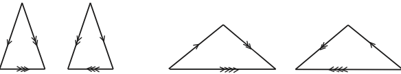
Figure 6.1. The tiles of the Penrose tiling.

The dynamical system $(\mathcal{T}(\mathcal{P}),\bar{\Theta})$ associated with Penrose tiles system is minimal and uniquely ergodic (see for instance [11]). Actually much more can be said about the ergodic properties of Penrose dynamical systems.
We recall that a van Hove sequence for $\mathbb{R}^{2}$ is a sequence $\{F_{n}\}_{n\geq 1}$ of bounded measurable subsets of $\mathbb{R}^{2}$ satisfying

$$\lim_{n\to\infty}\lambda\big{(}\big{(}\partial F_{n}\big{)}^{+r}\big{)}\big{/}\lambda(F_{n})=0,\;\textup{for all}\;r>0$$

where, for a subset $A$ of $\mathbb{R}^{2}$, $A^{+r}:=\big{\{}x\in\mathbb{R}^{2}:\textup{dist}(x,A)\leq r\big{\}}$.

Proposition 14.

Let $\lambda$ be the Lebesgue measure in $\mathbb{R}^{2}$ and consider a van Hove sequence $\{F_{n}\}_{n\geq 1}$ in $\mathbb{R}^{2}$. For any tiling $T$ in $\mathcal{T}(\mathcal{P})$, any $x$ in $\mathbb{R}^{2}$ and any $n\geq 1$, let $L^{\scriptscriptstyle{\textup{fat}}}_{T}(x+F_{n})$ (resp. $L^{\scriptscriptstyle{\textup{thin}}}_{T}(x+F_{n})$) be the number of fat (resp. thin) triangles of $T$ in $x+F_{n}$. Then the following limits

$$\nu(\textup{fat})=\lim_{n\to\infty}\frac{L^{\scriptscriptstyle{\textup{fat}}}_{T}(x+F_{n})}{\lambda(F_{n})}\quad\textup{and}\quad\nu(\textup{thin})=\lim_{n\to\infty}\frac{L^{\scriptscriptstyle{\textup{thin}}}_{T}(x+F_{n})}{\lambda(F_{n})}$$

exist, are independent of $T$ in $\mathcal{T}(\mathcal{P})$, $x$ in $\mathbb{R}^{2}$ and of the van Hove sequence $\{F_{n}\}_{n\geq 1}$, and satisfy:

$$\frac{\nu(\textup{fat})}{\nu(\textup{thin})}=\frac{1+\sqrt{5}}{2}.$$

The fact that the limits exist and are independent of the tiling, the reference point and the van Hove sequence, is a direct consequence of unique ergodicity as shown in [8, Theorem 2.7]. The fact that the ratio of these limits is the golden mean can be easily checked by choosing the van Hove sequence made with the series of successive inflations of a given triangle with respect to the substitution rules.

6.3. Wang tilings

A special class of tilings is that of Wang tilings, which we describe for $d=2$ for the sake of simplicity. A Wang prototile is a unit square with sides parallel to the axes, and with colored edges which restrict adjecency: abutting edges of adjacent tiles must have the same color. Consider a finite collection $W$ of Wang prototiles; it gives rise to the a tiling space consisting of all admissible tilings of the plane, i.e. tilings in which the adjecency rules are obeyed. Wang tilings are closely tied to shifts of finite type because, giving the tiling space, we can translate every tiling so that the vertices of its tiles lie on the lattice $\mathbb{Z}^{2}$. The resulting family of tilings can be identified with a collection of configurations in $W^{\mathbb{Z}^{2}}$, which is easily seen to be an SFT. Thus the tiling space is (conjugate to) the suspension of a shift of finite type $X_{W}$. This basic fact and its reciprocal was noticed in [16]. Let us also mention again Berger’s theorem: there is no algorithm which computes for a given $W$ whether the corresponding SFT is empty or, equivalently, whether $\mathcal{T}(W)=\emptyset$.

The importance of Wang tilings stems from the following result proved by Sadun and Williams [15] which we formulate here for $d=2$, although it is valid for any dimension: Let $\mathcal{P}$ be a finite set of prototiles and $\mathcal{T}(P)$ the associated tiling space. Then there exists a finite set of Wang prototiles $W$ and a homeomorphism $h$ which realizes an orbit equivalence between the dynamical systems $(\mathcal{T}(P),\bar{\Theta})$ and $(\mathcal{T}(W),\bar{\Theta})$. In particular, there exists a finite alphabet $W$ such that the tiling space $\mathcal{T}(P)$ is homeomorphic to the suspension of the $\mathbb{Z}^{2}$-SFT $X_{W}$.

6.4. From the Penrose tiling system to a uniquely ergodic SFT

An SFT can be explicitly constructed from the Penrose system, as shown in [15]. For the sake of convenience, we sketch the construction given therein in full details. The first step is to construct a rational tiling space from the original Penrose system by a homeomorphism. By a rational tiling we mean a tiling whose edge vectors all have rational coordinates. This amounts to solving finitely many equations with integral coefficients yielding the result by elementary linear algebra. By rescaling if necessary, we can assume that the obtained rational Penrose tiling is in fact integral and that each triangle contains at least one unit square whose corners have integer coordinates. Figure 6.2 displays a patch of the integral Penrose tiling.

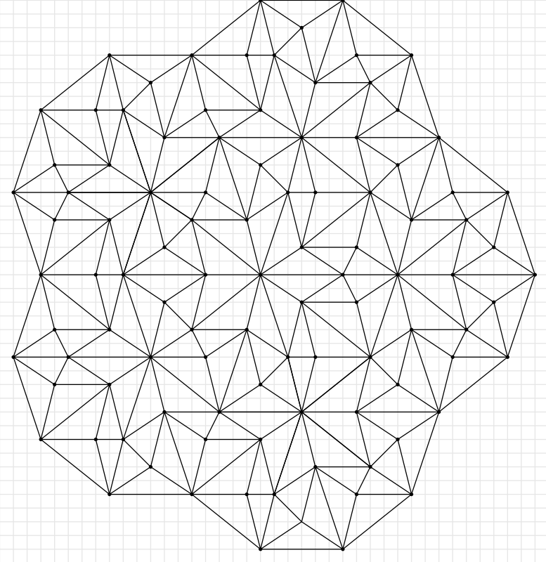
Figure 6.2. A patch of the rational Penrose tiling.

Let us denote by $\mathcal{P}_{\textup{int}}$ the new set of 40 triangles obtained this way and let us keep on calling thin and fat triangles the respective images of the thin and fat Penrose triangles. Clearly the new dynamical system $(\mathcal{T}(\mathcal{P}_{\textup{int}}),\bar{\Theta})$ is orbit equivalent to $(\mathcal{T}(\mathcal{P}),\bar{\Theta})$. The following proposition is a direct consequence of the fact that the homeomorphism that maps a Penrose tiling $T$ on a integral Penrose tiling $T_{\textup{int}}$, maps van Hove sequences on van Hove sequences.

Proposition 15.

The new dynamical system $(\mathcal{T}(\mathcal{P}_{\textup{int}}),\bar{\Theta})$ is again minimal and uniquely ergodic. Furtheremore, for any tiling $T_{\textup{int}}$ in $\mathcal{T}(\mathcal{P}_{\textup{int}})$, any $x$ in $\mathbb{R}^{2}$ and any $n\geq 1$, the following limits

$$\nu_{int}(\textup{fat})=\lim_{n\to\infty}\frac{L^{\scriptscriptstyle{\textup{fat}}}_{T_{int}}(x+F_{n})}{\lambda(F_{n})}\quad\textup{and}\quad\nu_{\textup{int}}(\textup{thin})=\lim_{n\to\infty}\frac{L^{\scriptscriptstyle{\textup{thin}}}_{T_{\textup{int}}}(x+F_{n})}{\lambda(F_{n})}$$

exist, are independent on ${T_{\textup{int}}}$ in $\mathcal{T}(\mathcal{P}_{\textup{int}})$, $x$ in $\mathbb{R}^{2}$ and on the van Hove sequence $\{F_{n}\}_{n\geq 1}$, and satisfy again:

$$\frac{\nu_{\textup{int}}(\textup{fat})}{\nu_{\textup{int}}(\textup{thin})}\,=\,\frac{1+\sqrt{5}}{2}.$$

The next step is to transform the rational Penrose tiling into a Wang tiling. The basic idea is to replace the straight edges of the triangles with zig-zags, that is with sequences of unit displacements in the coordinates directions. The next figure shows how the previous patch is transformed.

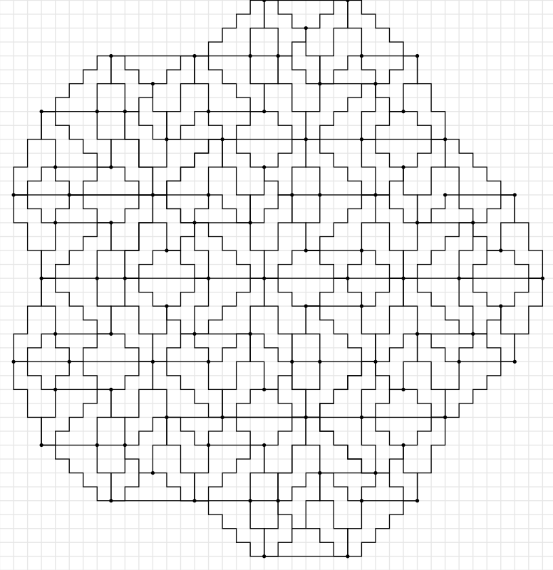
Figure 6.3. A patch of the square Penrose tiling.

It remains to put appropriate colors on the edges of the squares to obtain a Wang tiling. Colors are used to encode each of the $40$ prototiles and to encode the matching rules between them. Let $W$ be the set of $|W|$ Wang tiles constructed this way. Clearly the two dynamical systems $(\mathcal{T}(\mathcal{P}_{int}),\bar{\Theta})$ and $(\mathcal{T}(W),\bar{\Theta})$ are conjugate and thus $(\mathcal{T}(W),\bar{\Theta})$ is minimal and uniquely ergodic. In each triangle of $\mathcal{P}_{\textup{int}}$ choose one Wang tile. We get this way a collection of 20 distinct Wang tiles chosen in fat triangles: $W^{\scriptscriptstyle{\textup{fat}}}=\{w^{\scriptscriptstyle{\textup{fat}}}_{1},\dots,w^{\scriptscriptstyle{\textup{fat}}}_{20}\}$ and $20$ distinct Wang tiles chosen in thin triangles: $W^{\scriptscriptstyle{\textup{thin}}}=\{w^{\scriptscriptstyle{\textup{thin}}}_{1},\dots,w^{\scriptscriptstyle{\textup{thin}}}_{20}\}$. Let $\mu$ be the unique translation invariant measure of the associated SFT $X_{W}$. As a by-product of Proposition 15, we get:

$$\frac{\sum_{i=1}^{i=20}\mu([w^{\scriptscriptstyle{\textup{fat}}}_{i}])}{\sum_{i=1}^{i=20}\mu([w^{\scriptscriptstyle{\textup{thin}}}_{i}])}\,=\,\frac{1+\sqrt{5}}{2}.$$

Consequently there exists a pair $(i,j)$ in $\{1,\dots,20\}^{2}$ such that

$$\frac{\mu([w^{\scriptscriptstyle{\textup{fat}}}_{i}])}{\mu([w^{\scriptscriptstyle{\textup{thin}}}_{j}])}\,\notin\mathbb{Q}.$$

Thus we have construct a uniquely ergodic SFT on a finite alphabet with $|W|$ letters for which the ratio of the measures 2 cylinders with size 1 is irrational. This shows Theorem 6 for an alphabet with $|W|$ letters. By replacing individual symbols in $W$ by square words of fixed size written in any given finite alphabet with the property that that any subsequence of a concatenation of them has a unique parsing, we can show Theorem 6 for any finite alphabet.

References

- [1] N. Aubrun and M. Sablik. Simulation of effective subshifts by two-dimensional subshifts. preprint, 2010.
- [2] R. Berger. The undecidability of the domino problem. Mem. Amer. Math. Soc. No., 66:72, 1966.
- [3] Bruno Durand, Andrei Romashchenko, and Alexander Shen. Fixed-point tile sets and their applications. preprint, 2009.
- [4] H.-O. Georgii. Gibbs measures and phase transitions, volume 9 of de Gruyter Studies in Mathematics. Walter de Gruyter & Co., Berlin, 1988.
- [5] B. Grünbaum and G. C. Shephard. Tilings and patterns. A Series of Books in the Mathematical Sciences. W. H. Freeman and Company, New York, 1989. An introduction.
- [6] M. Hochman. On the dynamics and recursive properties of multidimensional symbolic systems. Invent. Math., 176(1):131–167, 2009.
- [7] M. Hochman and T. Meyerovitch. A characterization of the entropies of multidimensional shifts of finite type. Annals of Mathematics, 171(3):2011–2038, 2010.
- [8] J.-Y. Lee, R. Moody, and B. Solomyak. Pure point dynamical and diffraction spectra. Ann. Henri Poincaré, 3:1–17, 2002.
- [9] S. Mozes. Tilings, substitution systems and dynamical systems generated by them. J. Analyse Math., 53:139–186, 1989.
- [10] M. Pivato. Building a stationary stochastic process from a finite-dimensional marginal. Canad. J. Math., 53(2):382–413, 2001.
- [11] E. A. Robinson, Jr. The dynamical properties of Penrose tilings. Trans. Amer. Math. Soc., 348(11):4447–4464, 1996.
- [12] E. A. Robinson, Jr. Symbolic dynamics and tilings of . In Symbolic dynamics and its applications, volume 60 of Proc. Sympos. Appl. Math., pages 81–119. Amer. Math. Soc., Providence, RI, 2004.
- [13] R. M. Robinson. Undecidability and nonperiodicity for tilings of the plane. Invent. Math., 12:177–209, 1971.
- [14] D. Ruelle. Thermodynamic formalism. Cambridge Mathematical Library. Cambridge University Press, Cambridge, second edition, 2004. The mathematical structures of equilibrium statistical mechanics.
- [15] L. Sadun and R. F. Williams. Tiling spaces are Cantor set fiber bundles. Ergodic Theory Dynam. Systems, 23(1):307–316, 2003.
- [16] K. Schmidt. Multi-dimensional symbolic dynamical systems. In Codes, systems, and graphical models (Minneapolis, MN, 1999), volume 123 of IMA Vol. Math. Appl., pages 67–82. Springer, New York, 2001.
- [17] S. G. Simpson. Medvedev degrees of 2-dimensional subshifts of finite type. To appear in Ergod. Th. Dynam. Sys. (2011). Preprint available at www.math.psu.edu/simpson/papers/2dim.pdf.