Efficient Bayesian Inference for Switching State-Space Models using Discrete Particle Markov Chain Monte Carlo Methods

Abstract

Switching state-space models (SSSM) are a very popular class of time series models that have found many applications in statistics, econometrics and advanced signal processing. Bayesian inference for these models typically relies on Markov chain Monte Carlo (MCMC) techniques. However, even sophisticated MCMC methods dedicated to SSSM can prove quite inefficient as they update potentially strongly correlated discrete-valued latent variables one-at-a-time (Carter and Kohn, 1996; Gerlach et al., 2000; Giordani and Kohn, 2008). Particle Markov chain Monte Carlo (PMCMC) methods are a recently developed class of MCMC algorithms which use particle filters to build efficient proposal distributions in high-dimensions (Andrieu et al., 2010). The existing PMCMC methods of Andrieu et al. (2010) are applicable to SSSM, but are restricted to employing standard particle filtering techniques. Yet, in the context of discrete-valued latent variables, specialised particle techniques have been developed which can outperform by up to an order of magnitude standard methods (Fearnhead, 1998; Fearnhead and Clifford, 2003; Fearnhead, 2004). In this paper we develop a novel class of PMCMC methods relying on these very efficient particle algorithms. We establish the theoretical validy of this new generic methodology referred to as discrete PMCMC and demonstrate it on a variety of examples including a multiple change-points model for well-log data and a model for U.S./U.K. exchange rate data. Discrete PMCMC algorithms are shown to outperform experimentally state-of-the-art MCMC techniques for a fixed computational complexity. Additionally they can be easily parallelized (Lee et al., 2010) which allows further substantial gains.

Keywords: Bayesian inference, Markov chain Monte Carlo, optimal resampling, particle filters, sequential Monte Carlo, switching state-space models.

1 Introduction

Linear Gaussian Switching State-Space Models (SSSM) are a class of time series models in which the parameters of a linear Gaussian model switch according to a discrete latent process. They are ubiquitous in statistics (Cappé et al., 2005; Frühwirth-Schnatter, 2006), econometrics (Kim and Nelson, 1999; Giordani et al., 2007) and advanced signal processing (Barembruch et al., 2009; Costa et al., 2005) as they allow us to describe in a compact and interpretable way regime switching time series. SSSM have been successfully used to describe, among others, multiple change-point models (Fearnhead and Clifford, 2003; Giordani and Kohn, 2008), nonparametric regression models with outliers (Carter and Kohn, 1996) and Markov switching autoregressions (Billio and Monfort, 1998; Frühwirth-Schnatter, 2006; Kim and Nelson, 1999).

Performing Bayesian inference for SSSM requires the use of Markov chain Monte Carlo (MCMC) techniques. The design of efficient sampling techniques for this class of models has been a subject of active research for over fifteen years, dating back at least as far as Carter and Kohn (1994); Shephard (1994). A recent overview of MCMC in this context can be found in Cappé et al. (2005); Frühwirth-Schnatter (2006). The main practical difficulty lies in simulating from the conditional distribution of the trajectory of the discrete-valued latent process. The cost of computing this distribution grows exponentially in the length of the observation record and therefore obtaining an exact sample from it is impractical for all but tiny data sets. A standard strategy is instead to update the components of the discrete latent process one-at-a-time (Carter and Kohn, 1996; Gerlach et al., 2000; Giordani and Kohn, 2008). However, it is well-known that such an approach can significantly slow down the convergence of MCMC algorithms. An alternative is to sample approximately from the joint distribution of the latent discrete trajectory using particle filters: non-iterative techniques based on a combination of importance sampling and resampling techniques, see Doucet et al. (2001); Liu (2001) for a review of the literature. Empirical evidence suggests that particle filters are able to provide samples whose distribution is close to the target distribution of interest and this evidence is backed up by the rigourous quantitative bounds established in Del Moral (2004, chapter 8). This motivates using particle filters as proposal distributions within MCMC.

This idea is very natural, but its realization is far from trivial as the distribution of a sample generated by a particle filter does not admit a closed-form expression hence preventing us from directly using the standard Metropolis-Hastings (MH) algorithm. In a recent paper Andrieu et al. (2010) have shown that it is possible to bypass this problem. The authors have proposed a whole class of MCMC algorithms named Particle MCMC (PMCMC) relying on proposals built using particle filters. These algorithms have been demonstrated in the context of non-linear non-Gaussian state-space models and are directly applicable to SSSM; see also Flury and Shephard (2010) for applications in financial econometrics. However, the standard particle methods employed in Andrieu et al. (2010) do not fully exploit the discrete nature of the latent process in SSSM. This was recognized early by Paul Fearnhead who proposed an alternative generic algorithm, which we refer to as the Discrete Particle Filter (DPF) (Fearnhead, 1998). The DPF bypasses the importance sampling step of standard particle techniques and can be interpreted as using a clever random pruning mechanism to select support points from the exponentially growing sequence of discrete latent state spaces. The DPF methodology has been demonstrated successfully in a variety of applications (Cappé et al., 2005; Fearnhead, 1998; Fearnhead and Clifford, 2003; Fearnhead, 2004). It has been shown to significantly outperform alternative sophisticated approaches such as the Rao-Blackwellized particle filters developed in Chen and Liu (2000); Doucet et al. (2000, 2001) by up to an order of magnitude for a fixed computational complexity.

The main contribution of this article is to propose a novel class of PMCMC algorithms referred to as discrete PMCMC methods relying on the DPF for this important class of statistical models. The practical efficiency of the proposed methods relies on an original backward sampling procedure. We show that on a variety of applications this new generic methodology outperforms state-of-the-art MCMC algorithms for a fixed computational complexity. Moreover, as in the case of standard particle filters (Lee et al., 2010), the DPF can be parallelized easily. This suggests that even greater computational gains can be achieved.

The rest of the paper is organised as follows. In Section 2 we present the general class of SSSM considered in this paper and give an illustrative example. In Section 3, we discuss the intractability of exact inference in SSSM and present the DPF algorithm (Fearnhead, 1998; Fearnhead and Clifford, 2003; Fearnhead, 2004). Our presentation is slightly non-standard and explicitly introduces the random support sets generated by the algorithm. This allows us to describe the DPF precisely and compactly in a probabilistic way which proves useful to establish the validity of the proposed algorithms. We also review standard MCMC techniques used in this context. In Section 4 we introduce discrete PMCMC algorithms relying on the DPF to perform inference in SSSM and present some theoretical results. In Section 5, we review generic practical issues and demonstrate the efficiency of the proposed methods in the context of three examples. Finally in Section 6 we discuss several extensions of this work.

2 Switching state-space models

2.1 Model

From herein, we use the standard convention whereby capital letters are used for random variables while lower case letters are used for their values. Hereafter for any generic process $\left\{z_{n}\right\}$ we will denote $z_{i:j}:=\left(z_{i},z_{i+1},\ldots,z_{j}\right)$. The identity matrix of size $p$ is denoted $I_{p}$ and the matrix of zeros of size $p\times q$ by $0_{p\times q}$.

Consider the following SSSM, also known in the literature as a conditionally linear Gaussian state-space model or a jump linear system. The latent state process $\left\{X_{n}\right\}_{n\geq 1}$ is such that $X_{n}$ takes values in a finite set $\mathcal{X}$. It is characterized by its initial distribution $X_{1}\sim\nu_{\theta}\left(\cdot\right)$ and transition probabilities for $n>1$

$$X_{n}|(X_{1:n-1}=x_{1:n-1})\sim f_{\theta}\left(\cdot|x_{1:n-1}\right).$$ (1)

Conditional upon $\left\{X_{n}\right\}_{n\geq 1}$, we have a linear Gaussian state-space model defined through $Z_{0}\sim\mathcal{N}(m_{0},\Sigma_{0})$ and for $n\geq 1$

$$Z_{n} =A_{\theta}(X_{n})Z_{n-1}+B_{\theta}(X_{n})V_{n}+F_{\theta}(X_{n})u_{n},\text{ }$$ (2)

$$Y_{n} =C_{\theta}(X_{n})Z_{n}+D_{\theta}(X_{n})W_{n}+G_{\theta}(X_{n})u_{n},$$ (3)

where $\mathcal{N}(m,\Sigma)$ is the normal distribution of mean $m$ and covariance $\Sigma$, $V_{n}\overset{\text{i.i.d.}}{\sim}\mathcal{N}(0_{v\times 1},I_{v})$, $W_{n}\overset{\text{i.i.d.}}{\sim}\mathcal{N}(0_{w\times 1},I_{w})$, $\left\{A_{\theta}(x),B_{\theta}(x),C_{\theta}(x),D_{\theta}(x),F_{\theta}(x),G_{\theta}(x);x\in\mathcal{X}\right\}$ are matrices of appropriate dimension and $u_{n}$ is an exogeneous input. Here $\theta\in\Theta$ is some static parameter which may be multidimensional, for example $\Theta\subset\mathbb{R}^{d}$. For purposes of precise specification of resampling algorithms in the sequel and without loss of generality we label the elements of $\mathcal{X}$ with numbers, for example $\mathcal{X}=\left\{1,...,\mathcal{\left|X\right|}\right\}$ for some $\left|\mathcal{X}\right|\in\mathbb{N}$. We may then endow each Cartesian product space $\mathcal{X}^{2},\mathcal{X}^{3},...$ with the corresponding lexicographical order relation. From henceforth, whenever we refer to ordering of a set of points in $\mathcal{X}^{n}$ it is with respect to the latter relation.

We give here a simple example of a SSSM. Two more sophisticated examples are discussed in Section 5.

2.1.1 Example: Auto-regression with shifting level

Let $\mathcal{X}=\left\{0,1\right\}$ and for $\left\{X_{n}\right\}$ a Markov chain on $\mathcal{X}$ with transition matrix $P_{X}$, consider the process defined by

$$Y_{n} = \mu_{n}+\phi(Y_{n-1}-\mu_{n-1})+\sigma V_{n,1}$$

$$\mu_{n} = \mu_{n-1}+\sigma X_{n}V_{n,2},$$

where for each $n\geq 1$, $\mu_{n}$ and $Y_{n}$ are real-valued and $\left\{V_{n,1}\right\}$ and $\left\{V_{n,2}\right\}$ are i.i.d. $\mathcal{N}(0,1)$. The initial distribution on $\mu_{0}$ is $\mathcal{N}(m_{0},\sigma_{0}^{2})$ and is assumed known. This is a natural generalization of a first order autoregressive model to the case where the level $\mu_{n}$ is time-varying with shifts driven by the latent process $\left\{X_{n}\right\}$. This model can be expressed in state-space form by setting

$$Z_{n}=\left[\begin{array}[]{c}Y_{n}-\mu_{n}\\ \mu_{n}\end{array}\right],\quad A_{\theta}(x_{n})=\left[\begin{array}[]{cc}\phi&0\\ 0&1\end{array}\right]\quad\forall x_{n},$$

$$B_{\theta}(x_{n})=\sigma\left[\begin{array}[]{cc}1&0\\ 0&x_{n}\end{array}\right],\quad C_{\theta}(x_{n})=\left[\begin{array}[]{cc}1&1\end{array}\right],\quad D_{\theta}(x_{n})=F_{\theta}(x_{n})=G_{\theta}(x_{n})=0,\quad\forall x_{n}.$$

The unknown parameters of this model are $\theta=[\phi\;\sigma^{2}\;P_{X}]$ where $P_{X}$ is the transition matrix of $\{X_{n}\}$. In this model and more generally in SSSMs, inferences about the latent processes $\left\{\mu_{n}\right\}$ and $\left\{X_{n}\right\}$ from a particular data set are likely to be highly sensitive to values of these parameters if they are assumed known.

2.2 Inference aims

Our aim is to perform Bayesian inference in SSSMs, conditional upon some observations $y_{1:T}$ and for some $T\geq 1$, treating both the latent trajectories $X_{1:T},Z_{0:T}$ and the parameter $\theta$ as unknowns. Where applicable, the values of the input sequence $u_{1:T}$ are assumed known, but for clarity we suppress them from our notation. We ascribe a prior density $p\left(\theta\right)$ to $\theta$ so Bayesian inference relies on the joint density

$$p\left(\theta,x_{1:T},z_{0:T}|y_{1:T}\right)\propto p_{\theta}\left(x_{1:T},z_{0:T},y_{1:T}\right)p\left(\theta\right),$$ (4)

where the definition of $p_{\theta}\left(x_{1:T},z_{0:T},y_{1:T}\right)$ follows from Eq. (1)-(2)-(3). This posterior can be factorized as follows

$$p\left(\theta,x_{1:T},z_{0:T}|y_{1:T}\right)=p\left(\theta,x_{1:T}|y_{1:T}\right)p_{\theta}\left(z_{0:T}|y_{1:T},x_{1:T}\right)$$ (5)

where

$$p\left(\theta,x_{1:T}|y_{1:T}\right)=\dfrac{p_{\theta}\left(y_{1:T}|x_{1:T}\right)p(x_{1:T}|\theta)p(\theta)}{\int_{\Theta}\sum_{x_{1:T}^{\prime}\in\mathcal{X}^{T}}p_{\theta}\left(y_{1:T}|x_{1:T}^{\prime}\right)p(x_{1:T}^{\prime}|\theta)p\left(\theta\right)\mathrm{d}\theta}.$$ (6)

Conditional upon $X_{1:T}=x_{1:T},$ Eq. (2)-(3) define a linear Gaussian state-space model so it is possible to compute efficiently the statistics of the conditional multivariate Gaussian density $p_{\theta}\left(\left.z_{0:T}\right|y_{1:T},x_{1:T}\right)$ in Eq. (5) and the conditional marginal likelihood $p_{\theta}\left(\left.y_{1:T}\right|x_{1:T}\right)$ in Eq. (6) using Kalman techniques. For example $p_{\theta}\left(\left.y_{1:T}\right|x_{1:T}\right)$ can be computed using the product of predictive densities

$$p_{\theta}\left(\left.y_{1:T}\right|x_{1:T}\right)={\displaystyle\prod\limits_{n=1}^{T}}g_{\theta}\left(\left.y_{n}\right|y_{1:n-1},x_{1:n}\right)$$ (7)

where $y_{1:0}:=\varnothing$. The statistics of these Gaussian predictive densities can be computed using the Kalman filter which is recalled in Appendix A for sake of convenience. For simplicity of presentation throughout the following we assume that for each $1\leq n\leq T$ and $\theta\in\Theta$ the support of $p_{\theta}\left(x_{1:n}\left|y_{1:n}\right.\right)$ is $\mathcal{X}^{n}$. This assumption is satisfied in the vast majority of cases considered in practice and in all the examples we consider. The techniques discussed below can be transferred to cases where this assumption is not met with only cosmetic changes.

3 Inference techniques for switching state-space models

3.1 Exact Inference and Intractability

The main difficulty faced in the exact computation of $p(\theta,x_{1:T}|y_{1:T})$, is the need to perform the summation in the denominator of Eq. (6) over up to $\left|\mathcal{X}\right|^{T}$ values of $x_{1:T}$, where $\left|\mathcal{X}\right|$ is the cardinality of $\mathcal{X}$. For even modest values of $T$, this sum is too expensive to compute exactly. In the applications we consider, $T$ is of the order of thousands, so exact computation is practically impossible.

Even if $\theta$ is treated as fixed, inference is intractable. In this case, we wish to compute $p_{\theta}(x_{1:T}|y_{1:T})$, whose normalization involves the same problematic summation. One approach is to obtain $p_{\theta}(x_{1:T}|y_{1:T})$ by sequential computation of $p_{\theta}(x_{1}|y_{1}),p_{\theta}(x_{1:2}|y_{1:2}),...$ via the recursive relationship

$$p_{\theta}(x_{1:n}|y_{1:n})=\dfrac{g_{\theta}(y_{n}|y_{1:n-1},x_{1:n})f_{\theta}(x_{n}|x_{1:n-1})p_{\theta}(x_{1:n-1}|y_{1:n-1})}{\sum_{x_{1:n\in\mathcal{X}^{n}}}g_{\theta}(y_{n}|y_{1:n-1},x_{1:n})f_{\theta}(x_{n}|x_{1:n-1})p_{\theta}(x_{1:n-1}|y_{1:n-1})},$$

(with $g_{\theta}(y_{n}|y_{1:n-1},x_{1:n})$ the predictive as defined in the previous section) but the computation involved increases exponentially in $n$. For purposes of exposition in the sequel, we remark that, as for each $n$ the support of $p_{\theta}(x_{1:n}|y_{1:n})$ is $\mathcal{X}^{n}$ then the sequence of such supports satisfies the trivial recursion

$$\mathcal{X}^{n}=\mathcal{X}\times\mathcal{X}^{n-1},$$

and is evidently growing in cardinality with $n$. Hence, in both the cases of computing $p(\theta,x_{1:T}|y_{1:T})$ and $p_{\theta}(x_{1:T}|y_{1:T})$ it is necessary to rely on approximations and we focus here on Monte Carlo methods.

3.2 Monte Carlo Methods

We next review two classes of Monte Carlo techniques to perform inference in SSSM. The first method we discuss is the DPF algorithm of Fearnhead (1998). For a fixed parameter value $\theta$, this algorithm allows us to compute an approximation of the posterior distribution $p_{\theta}\left(x_{1:T}|y_{1:T}\right)$ and an approximation of the marginal likelihood $p_{\theta}\left(y_{1:T}\right)$. We present this algorithm in a slightly non-standard way which allows us to describe it probabilistically in a concise and precise manner. This will prove useful for the development of the discrete PMCMC algorithms in Section 4. We also review MCMC methods which have been developed to approximate $p\left(\theta,x_{1:T},z_{0:T}|y_{1:T}\right)$ and discuss their advantages and limitations.

3.3 The discrete particle filter

The DPF algorithm proposed in Fearnhead (1998); Fearnhead and Clifford (2003) is a non-iterative procedure approximating the posterior distribution $p_{\theta}\left(x_{1:T}|y_{1:T}\right)$ and the marginal likelihood $p_{\theta}\left(y_{1:T}\right)$. Practically, the DPF approximation of the posterior distributions $\left\{p_{\theta}\left(x_{1:n}|y_{1:n}\right);n\geq 1\right\}$ is made sequentially in time using a collection of $N\left|\mathcal{X}\right|$ weighted trajectories or “particles” $\left\{X_{1:n}^{\left(i\right)};i=1,...,N\left|\mathcal{X}\right|\right\}$,

$$\widehat{p}_{\theta}^{N}\left(x_{1:n}|y_{1:n}\right)=\sum_{i=1}^{N\left|\mathcal{X}\right|}W_{n}^{\theta}\left(X_{1:n}^{\left(i\right)}\right)\delta_{X_{1:n}^{\left(i\right)}}\left(x_{1:n}\right),\text{ }W_{n}^{\theta}\left(X_{1:n}^{\left(i\right)}\right)\geq 0,\text{ }\sum_{i=1}^{N\left|\mathcal{X}\right|}W_{n}^{\theta}\left(X_{1:n}^{\left(i\right)}\right)=1.$$

The parameter $N$ controls the precision of the algorithm. The larger it is, the more accurate (on average) the approximation of the target distribution. It has been demonstrated experimentally in Cappé et al. (2005); Fearnhead and Clifford (2003); Fearnhead (2004) that the DPF algorithm outperforms significantly, sometimes by one order of magnitude, the Rao-Blackwellized particle filters proposed in Chen and Liu (2000); Doucet et al. (2000, 2001) and that it is able to provide very good approximations of $p_{\theta}\left(x_{1:T}|y_{1:T}\right)$ in realistic scenarios even with a moderate number of particles. The action of the DPF can be summarised as follows.

Assume that we have, at time step $n$ obtained $\widehat{p}_{\theta}^{N}\left(x_{1:n}|y_{1:n}\right)$ consisting of $N\left|\mathcal{X}\right|$ distinct particles with weights that sum to 1. A resampling step is then applied, exactly $N$ of the $N|\mathcal{X}|$ trajectories survive and their weights are adjusted accordingly. The resampling mechanism is chosen in such a way as to be optimal in some sense. Throughout the remainder of the paper we treat the case of minimising the sum of variances of the importance weights as in Fearnhead and Clifford (2003) but exactly the same method applies to other schemes discussed in Barembruch et al. (2009). Features of this resampling scheme which distinguish it from standard methods, such as multinomial resampling, are that it results in no duplicated particles and gives post-resampling weights which are non-uniform.

Whereas standard particle methods rely on a stochastic proposal mechanism to explore the space, the DPF performs all its exploration deterministically. This is possible because of the finite cardinality of the latent discrete space. Consider one of $N$ particles which survived the resampling operation, each of which is a point in $\mathcal{X}^{n}$. Call the point in question $x_{1:n}$ and denote by $m_{n|n}^{z,\theta}(x_{1:n})$ and $\Sigma_{n|n}^{z,\theta}(x_{1:n})$ respectively the mean and covariance of the Gaussian density $p_{\theta}(z_{n}|y_{1:n},x_{1:n})$. From this point $|\mathcal{X}|$ new particles $\{(x_{1:n},x);x\in\mathcal{X}\}$ are formed, and for each one of them, $m_{n+1|n+1}^{z,\theta}(x_{1:n},x)$, $\Sigma_{n+1|n+1}^{z,\theta}(x_{1:n},x)$ and the associated unnormalized weight are calculated using the Kalman filtering recursions (included for reference in Appendix A). This procedure is repeated for the remaining $N-1$ particles, resulting in $N|\mathcal{X}|$ weighted trajectories. The weights are then normalized to yield a probability distribution constituting $\widehat{p}_{\theta}^{N}\left(x_{1:n+1}|y_{1:n+1}\right)$.

This outline of the DPF operations highlights the function of the resampling step: in the case of the DPF it acts to prune the exponentially growing (in $n$) tree of possible paths $\left\{x_{1:n}\in\mathcal{X}^{n};n=1,2,...\right\}$. It is convenient to specify the DPF in a slightly non-standard way which highlights that the only randomness in this algorithm arises from the resampling step. To this end, we introduce random support sets $\mathbf{S}_{1},\mathbf{S}_{2},...,\mathbf{S}_{T}$ with each $\mathbf{S}_{n}$ taking a value $\mathbf{s}_{n}$ which is a subset of $\mathcal{X}^{n}$. It is stressed that, in the following interpretation, the $x_{1:n}$’s are not random variables, and are just points in the state space (and Cartesian products thereof) used for indexing. With this notation, we write the DPF approximation for $n>1$ as

$$\widehat{p}_{\theta}^{N}\left(x_{1:n}|y_{1:n}\right) =\sum_{x_{1:n}^{\prime}\in\mathbf{S}_{n}}W_{n}^{\theta}\left(x_{1:n}^{\prime}\right)\delta_{x_{1:n}^{\prime}}\left(x_{1:n}\right).$$ (8)

Under the probability law of the DPF algorithm, which we discuss in more detail later, for each $n\geq 2$, $|\mathbf{S}_{n}|=N|\mathcal{X}|\wedge\left|\mathcal{X}^{n}\right|$, with probability $1$. We thus see in Eq. (8) the effect of the parameter $N$: it specifies the number of support points of the approximation $\widehat{p}_{\theta}^{N}\left(x_{1:n}|y_{1:n}\right)$. We next provide pseudo code for the DPF algorithm and then go on to discuss several issues related to its practical use and its theoretical representation.

 

DPF algorithm

At time $n=1$

$\bullet$ Set $\mathbf{S}_{1}=\mathcal{X}$ and for each $x_{1}\in\mathcal{X}$, compute $m_{1|1}^{z,\theta}(x_{1})$ , $\Sigma_{1|1}^{z,\theta}(x_{1})$ and $g_{\theta}(y_{1}|x_{1})$ using the Kalman filter.

$\bullet$ Compute and normalise the weights. For each $x_{1}\in\mathcal{X}$,

$$\overline{w}_{1}^{\theta}\left(x_{1}\right)=\nu_{\theta}\left(x_{1}\right)g_{\theta}\left(\left.y_{1}\right|x_{1}\right),\text{ }W_{1}^{\theta}\left(x_{1}\right)=\frac{\overline{w}_{1}^{\theta}\left(x_{1}\right)}{{\textstyle\sum\nolimits_{x_{1}^{\prime}\in\mathcal{X}}}\overline{w}_{1}^{\theta}\left(x_{1}^{\prime}\right)}.$$ (9)

At times $n=2,...,T$

$\bullet$ If $\left|\mathbf{S}_{n-1}\right|\leq N$ set $C_{n-1}=\infty$ otherwise set $C_{n-1}$ to the unique solution of

$$\sum_{x_{1:n-1}\in\mathbf{S}_{n-1}}1\wedge C_{n-1}W_{n-1}^{\theta}\left(x_{1:n-1}\right)=N.$$

$\bullet$ Maintain the $L_{n-1}$ trajectories in $\mathbf{S}_{n-1}$ which have weights strictly superior to $1/C_{n-1}$, then apply the stratified resampling mechanism to the other $N\left|\mathcal{X}\right|-L_{n-1}$ trajectories to yield $N-L_{n-1}$ survivors. Set $\mathbf{S}_{n-1}^{\prime}$ to the set of surviving and maintained trajectories.

$\bullet$ Set $\mathbf{S}_{n}=\mathbf{S}_{n-1}^{\prime}\times\mathcal{X}$.

$\bullet$ For each $x_{1:n}\in\mathbf{S}_{n}$, compute $m_{n|n}^{z,\theta}(x_{1:n})$ , $\Sigma_{n|n}^{z,\theta}(x_{1:n})$ and $g_{\theta}(y_{n}|y_{1:n-1},x_{1:n})$ using the Kalman filter.

$\bullet$ Compute and normalise the weights. For each $x_{1:n}\in\mathbf{S}_{n},$

$$\overline{w}_{n}^{\theta}\left(x_{1:n}\right) =f_{\theta}(x_{n}|x_{1:n-1})g_{\theta}(y_{n}|y_{1:n-1},x_{1:n})\dfrac{W_{n-1}^{\theta}\left(x_{1:n-1}\right)}{1\wedge C_{n-1}W_{n-1}^{\theta}\left(x_{1:n-1}\right)},$$ (10)

$$W_{n}^{\theta}\left(x_{1:n}\right) =\frac{\overline{w}_{n}^{\theta}\left(x_{1:n}\right)}{{\textstyle\sum\nolimits_{x_{1:n}^{\prime}\in\mathbf{S}_{n}}}\overline{w}_{n}^{\theta}\left(x_{1:n}^{\prime}\right)}.$$ (11)

 

3.3.1 Exact computation at the early iterations

For small $n$ it is practically possible to compute $p_{\theta}(x_{1:n}|y_{1:n})$ exactly. It is only once $n$ is large enough that $\left|\mathcal{X}^{n}\right|>N$ that we need to employ the resampling mechanism to prune the set of trajectories. This action is represented conceptually in the DPF algorithm above by the artifice of setting $C_{n}=\infty$ if $n$ is such that $\left|\mathbf{S}_{n-1}\right|\leq N$. When this condition is satisfied, the resampling step is not called into action. Of course in the practically unrealistic case that $\left|\mathcal{X}^{T}\right|\leq N$ the DPF, unlike standard SMC algorithms, thus reduces to exact recursive computation of $\left\{p_{\theta}(x_{1:n}|y_{1:n});n=1,...,T\right\}$.

3.3.2 Computing $C_{n}$ and stratified resampling

The threshold $C_{n}$ is a deterministic function of the weights $\left\{W_{n}^{\theta}\left(x_{1:n}\right)\right\}_{x_{1:n}\in\mathbf{S}_{n}}$. A method for solving $\sum_{x_{1:n}\in\mathbf{S}_{n}}1\wedge C_{n}W_{n}^{\theta}\left(x_{1:n}\right)=N$ is given in Fearnhead and Clifford (2003). The stratified resampling mechanism, which is employed once $C_{n}$ has been computed, proceeds as follows at time $n$; this was originally proposed in Carpenter et al. (1999); Kitagawa (1996), although not in the context of the DPF.

 

Stratified resampling

$\bullet$ Normalise the weights $\overline{w}_{n-1}^{\theta}\left(x_{1:n-1}\right)$ of the $N\left|\mathcal{X}\right|-L_{n-1}$ particles and label them according to the order of the corresponding $x_{1:n-1}$ to obtain $\widehat{W}_{n-1}^{\theta}\left(x_{1:n-1}^{\left(i\right)}\right)$; $i=1,...,N\left|\mathcal{X}\right|-L_{n-1}.$

$\bullet$ Construct the corresponding cumulative distribution function: for $i=1,...,N\left|\mathcal{X}\right|-L_{n-1}$,

$$Q_{n-1}^{\theta}(i):=\sum_{j\leq i}\widehat{W}_{n-1}^{\theta}\left(x_{1:n-1}^{\left(j\right)}\right),\qquad Q_{n-1}^{\theta}(0):=0.$$

$\bullet$ Sample $U_{1}$ uniformly on $\left[0,1/(N-L_{n-1})\right]$ and set $U_{j}=U_{1}+\frac{j-1}{N-L_{n-1}}$ for $j=2,...,N-L_{n-1}.$

$\bullet$ For $i=1,...,N\left|\mathcal{X}\right|-L_{n-1}$, if there exists $j\in\left\{1,...,N-L_{n-1}\right\}$ such that $Q_{n-1}^{\theta}(i-1)<U_{j}\leq Q_{n-1}^{\theta}(i)$, then $x_{1:n-1}^{(i)}$ survives.

 

3.3.3 Computational Requirements

Assuming that the cost of evaluating $f_{\theta}(x_{n}|x_{1:n-1})$ is $\mathcal{O}(1)$ for all $n$, the computational complexity of the DPF is $\mathcal{O}(|\mathcal{X}|N)$ at each time step due to the propagation of $N|\mathcal{X}|$ Kalman filtering operations and the generation of a single uniform random variable. The parallelisation techniques described in Lee et al. (2010) could readily be exploited when performing the Kalman computations.

3.3.4 Estimating $p_{\theta}\left(y_{1:T}\right)$

Of particular interest in the sequel is the fact that the DPF provides us with an estimate of the marginal likelihood $p_{\theta}\left(y_{1:T}\right)$ given by

$$\widehat{p}_{\theta}\left(y_{1:T}\right):=\widehat{p}_{\theta}\left(y_{1}\right){\displaystyle\prod\limits_{n=2}^{T}}\widehat{p}_{\theta}\left(y_{n}|y_{1:n-1}\right)$$ (12)

where

$$\widehat{p}_{\theta}\left(y_{1}\right)=\sum_{x_{1}\in\mathcal{X}}\overline{w}_{1}^{\theta}\left(x_{1}\right),\;\;\;\;\widehat{p}_{\theta}\left(y_{n}|y_{1:n-1}\right)=\sum_{x_{1:n}\in\mathbf{S}_{n}}\overline{w}_{n}^{\theta}\left(x_{1:n}\right),\;\;n>1.$$ (13)

Inevitably, for fixed $N$, the quality of the particle approximation to the distribution $p_{\theta}\left(x_{1:T}|y_{1:T}\right)$ decreases as $T$ increases. For fixed $T$, once $N$ is larger than $\left|\mathcal{X}^{T}\right|$, the DPF computes $p_{\theta}\left(y_{1:T}\right)$ exactly.

Before introducing the details of the new PMCMC algorithms, we review some existing MCMC algorithms for performing inference in SSSM.

3.4 Standard Markov chain Monte Carlo methods

Designing efficient MCMC algorithms to sample from $p\left(\theta,x_{1:T},z_{0:T}|y_{1:T}\right)$ is a difficult task. Most existing MCMC methods approach this problem using some form of Gibbs sampler and can be summarized as cycling in some manner through the sequence of distributions $p\left(\theta|y_{1:T},x_{1:T},z_{0:T}\right)$, $p_{\theta}\left(z_{0:T}|y_{1:T},x_{1:T}\right)$ and $p_{\theta}\left(x_{1:T}|y_{1:T},z_{0:T}\right)$ or $p_{\theta}\left(x_{1:T}|y_{1:T}\right)$.

Sampling efficiently from $p\left(\theta|y_{1:T},x_{1:T},z_{0:T}\right)$ is often feasible due to the small or moderate size of $\theta$ and the fact that for many models and parameters of interest, conjugate priors are available. When conjugate priors are not used, Metropolis-within-Gibbs steps may be applied.

A variety of efficient algorithms have been developed to sample from $p_{\theta}\left(z_{0:T}|y_{1:T},x_{1:T}\right)$. These methods rely on the conditionally linear Gaussian structure of the model and involve some form of forward filtering backward sampling recursion (Carter and Kohn, 1994; Frühwirth-Schnatter, 1994). Variants of these schemes which approach the task by explicitly sampling the state disturbances may be more efficient and/or numerically stable for some classes of models (De Jong and Shephard, 1995; Durbin and Koopman, 2002). In all the numerical examples we consider, sampling from $p_{\theta}\left(z_{0:T}|y_{1:T},x_{1:T}\right)$ was performed using the simulation smoother of Durbin and Koopman (2002).

Sampling from $p_{\theta}\left(x_{1:T}|y_{1:T},z_{0:T}\right)$ can also be performed efficiently using a forward filtering backward sampling recursion (Carter and Kohn, 1994; Chib, 1996) when $\left\{X_{n}\right\}$ is a Markov chain. The resulting Gibbs sampler is elegant but it can mix very slowly as $X_{1:T}$ and $Z_{0:T}$ are usually strongly correlated. To bypass this problem, Carter and Kohn (1996); Gerlach et al. (2000) proposed to integrate out $Z_{0:T}$ using the Kalman filter as discussed in Subsection 2.2. However, as mentioned in the introduction, exact sampling from $p_{\theta}\left(x_{1:T}|y_{1:T}\right)$ is typically infeasible as the cost of computing this distribution is exponential in $T$. Therefore, in the algorithms of Carter and Kohn (1996); Gerlach et al. (2000), the discrete variables $X_{1:T}$ are updated one-at-a-time according to their full conditional distributions $p_{\theta}\left(x_{n}|y_{1:T},x_{1:n-1},x_{n+1:T}\right)$. It was shown in Carter and Kohn (1996); Gerlach et al. (2000) that this strategy can improve performance drastically compared to algorithms where $X_{1:T}$ is updated conditional upon $Z_{0:T}$. From hereon we refer to the Gibbs sampler of Gerlach et al. (2000) as the “standard Gibbs” algorithm.

At this stage, we comment a little further on the method of Gerlach et al. (2000) as it is relevant to the new algorithms described in the later sections. The Gibbs sampler of Gerlach et al. (2000) achieves a sweep of samples from $p_{\theta}\left(x_{1}|y_{1:T},x_{2:T}\right)$, $p_{\theta}\left(x_{2}|y_{1:T},x_{1},x_{3:T}\right)$, etc. by a “backward–forward” procedure exploiting the identities

$$p_{\theta}\left(x_{n}|y_{1:T},x_{1:n-1},x_{n+1:T}\right)\propto p_{\theta}(y_{n}|y_{1:n-1},x_{1:n})p_{\theta}(x_{n}|x_{1:n-1},x_{n+1:T})p_{\theta}(y_{n+1:T}|y_{1:n},x_{1:T}),$$ (14)

and

$$p_{\theta}(y_{n+1:T}|y_{1:n},x_{1:T})=\int p_{\theta}(y_{n+1:T}|z_{n},x_{n+1:T})p_{\theta}(z_{n}|x_{1:n},y_{1:n})dz_{n}.$$ (15)

In Gerlach et al. (2000), it was shown that the coefficients of $z_{n}$ in $p_{\theta}(y_{n+1:T}|z_{n},x_{n+1:T})$ which are needed to evaluate (15) can be computed recursively for $n=T,T-1,...,1$ (the backward step). Then, for each $n=1,2,...,T$, $p_{\theta}(y_{n}|y_{1:n-1},x_{1:n})$ and $p_{\theta}(z_{n}|x_{1:n},y_{1:n})$ are obtained through standard Kalman filtering recursions, (15) is computed for each $x_{n}\in\mathcal{X}$ and a draw is made from (14) (the forward step). In the resulting algorithm, if the computational cost of evaluating $p_{\theta}(x_{n}|x_{1:n-1},x_{n+1:T})$ is $\mathcal{O}(1)$, the cost of one sampling sweep through $p_{\theta}\left(x_{1}|y_{1:T},x_{2:T}\right)$, $p_{\theta}\left(x_{2}|y_{1:T},x_{1},x_{3:T}\right)$, etc. grows linearly is $\mathcal{O}(T)$.

More recently, adaptive MCMC methods have been suggested to make one-at-a-time updates (Giordani and Kohn, 2008). However, these algorithms are still susceptible to slow mixing if the components of $X_{1:T}$ are strongly correlated. Moreover even if we were able to sample efficiently using one-at-a-time updates, this algorithm might still converge slowly if $X_{1:T}$ and $\theta$ are strongly correlated; e.g. if $\left\{X_{n}\right\}$ is a Markov chain and $\theta$ includes the transition matrix of this chain. Hammer and Tjelmeland (2011) have suggested an approximate, deterministic algorithm for forward filtering-backward smoothing in switching state space models, and the use of this method for making independent proposals as part of a Metropolis-Hastings scheme. By contrast, and as we shall see in the following section, the stochastic nature of the DPF algorithm allows the construction not only of exact Metropolis-Hastings-type algorithms, but also exact Particle Gibbs samplers. It is not clear how to achieve the latter using the deterministic forward-backward algorithm of Hammer and Tjelmeland (2011).

4 Discrete particle Markov chain Monte Carlo methods for switching state-space models

A natural idea arising from the previous section is to use the output $\widehat{p}_{\theta}\left(x_{1:T}|y_{1:T}\right)$ of the DPF algorithm as part of a proposal distribution for a MCMC algorithm targeting $p_{\theta}\left(x_{1:T}|y_{1:T}\right)$ or $p\left(\theta,x_{1:T}|y_{1:T}\right)$. This could allow us, in principle, to design automatically an efficient high-dimensional proposal for MCMC. However a direct application of this idea would require us to be able to both sample from and evaluate pointwise the unconditional distribution of a particle sampled from $\widehat{p}_{\theta}\left(x_{1:T}|y_{1:T}\right)$. This distribution is given by

$$q_{\theta}\left(x_{1:T}|y_{1:T}\right)=\mathbb{E}\left[\widehat{p}_{\theta}\left(x_{1:T}|y_{1:T}\right)\right],$$

where the expectation is with respect to the probability law of the DPF algorithm: the stochasticity which produces the random probability measure $\widehat{p}_{\theta}\left(x_{1:T}|y_{1:T}\right)$ in Eq. (8). While sampling from $q_{\theta}\left(x_{1:T}|y_{1:T}\right)$ is straightforward as it only requires running the DPF algorithm to obtain $\widehat{p}_{\theta}\left(x_{1:T}|y_{1:T}\right)$ then sampling from this random measure, the analytical expression for this distribution is clearly not available.

The novel MCMC updates presented in this section, under the umbrella term discrete PMCMC, circumvent this problem by considering target distributions on an extended space, over all the random variables of the DPF algorithm. Details of their theoretical validity are given in Subsection 4.3 but are not required for implementation of the algorithms. The key feature of these discrete PMCMC algorithms is that they are “exact approximations” to standard MCMC updates targeting $p\left(\theta,x_{1:T}|y_{1:T}\right)$. More precisely, on the one hand these algorithms can be thought of as approximations to possibly “idealized” standard MH updates parametrized by the number $N$ of particles used to construct the DPF approximation. On the other hand, under mild assumptions, discrete PMCMC algorithms are guaranteed to generate asymptotically (in the number of MCMC iterations used) samples from $p\left(\theta,x_{1:T}|y_{1:T}\right)$, for any fixed number $N\geq 2$ of particles, in other words, for virtually any degree of approximation.

In Subsection 4.1, we describe the Particle MMH (Marginal Metropolis-Hastings) algorithm which can be thought of as an exact approximation of an idealised “Marginal MH” (MMH) targeting directly the marginal distribution $p\left(\theta|y_{1:T}\right)$ of $p\left(\theta,x_{1:T}|y_{1:T}\right)$. This algorithm admits a form similar to the PMMH discussed in Andrieu et al. (2010) but its validity relies on different arguments. In Subsection 4.2 we present a particle approximation of a Gibbs sampler targeting $p\left(\theta,x_{1:T}|y_{1:T}\right)$, called the Particle Gibbs (PG) algorithm. It is a particle approximation of the “ideal” block Gibbs sampler which samples from $p\left(\theta,x_{1:T}|y_{1:T}\right)$ by sampling iteratively from the full conditionals $p_{\theta}\left(x_{1:T}|y_{1:T}\right)$ and $p\left(\theta|y_{1:T},x_{1:T}\right)$. This algorithm is significantly different from the PG sampler presented in Andrieu et al. (2010) and incorporates a novel backward sampling mechanism. Convergence results for these algorithms are established in Subsection 4.3.

4.1 Particle marginal Metropolis-Hastings sampler

Let us consider the following ideal “marginal” MH (MMH) algorithm to sample from $p\left(\theta,x_{1:T}|y_{1:T}\right)$ where $\theta$ and $x_{1:T}$ are updated simultaneously using the proposal given by

$$q\left(\left.\left(\theta^{\ast},x_{1:T}^{\ast}\right)\right|\left(\theta,x_{1:T}\right)\right)=q\left(\left.\theta^{\ast}\right|\theta\right)p_{\theta^{\ast}}\left(x_{1:T}^{\ast}|y_{1:T}\right)\ .$$

In this scenario the proposed $X{}_{1:T}^{\ast}$ is perfectly “adapted” to the proposed $\theta^{\ast}$ and the resulting MH acceptance ratio is given by

$$\frac{p\left(\theta^{\ast},x_{1:T}^{\ast}|y_{1:T}\right)}{p\left(\theta,x_{1:T}|y_{1:T}\right)}\frac{q\left(\left.\left(\theta,x_{1:T}\right)\right|\left(\theta^{\ast},x_{1:T}^{\ast}\right)\right)}{q\left(\left.\left(\theta^{\ast},x_{1:T}^{\ast}\right)\right|\left(\theta,x_{1:T}\right)\right)}=\frac{p_{\theta^{\ast}}\left(y_{1:T}\right)\text{ }p\left(\theta^{\ast}\right)}{p_{\theta}\left(y_{1:T}\right)\text{ }p\left(\theta\right)}\frac{q\left(\theta|\theta^{\ast}\right)}{q\left(\theta^{\ast}|\theta\right)}\ .$$ (16)

This algorithm is equivalent to a MH update working directly on the marginal density $p\left(\theta|y_{1:T}\right)$, justifying the MMH terminology. This algorithm is appealing but typically cannot be implemented as the marginal likelihood terms $p_{\theta}\left(y_{1:T}\right)$ and $p_{\theta^{\ast}}\left(y_{1:T}\right)$ cannot be computed exactly and it is impossible to sample exactly from $p_{\theta^{\ast}}\left(x_{1:T}|y_{1:T}\right)$. We propose the following particle approximation of the MMH algorithm where, whenever a sample from $p_{\theta}\left(x_{1:T}|y_{1:T}\right)$ and the expression for the marginal likelihood $p_{\theta}\left(y_{1:T}\right)$ are needed, their DPF approximation counterparts are used instead.

 

PMMH sampler for SSSM

Initialisation, $i=0$

$\bullet$ Set $\theta(0)$ arbitrarily.

$\bullet$ Run the DPF targeting $p_{\theta(0)}\left(x_{1:T}|y_{1:T}\right)$, sample $X_{1:T}\left(0\right)\sim\widehat{p}_{\theta(0)}\left(\cdot|y_{1:T}\right)$ and denote $\widehat{p}_{\theta(0)}\left(y_{1:T}\right)$

the marginal likelihood estimate.

For iteration $i\geq 1$

$\bullet$ Sample $\theta^{\ast}\sim q\left(\cdot|\theta\left(i-1\right)\right)$.

$\bullet$ Run the DPF targeting $p_{\theta^{\ast}}\left(x_{1:T}|y_{1:T}\right)$, sample $X_{1:T}^{\ast}\sim\widehat{p}_{\theta^{\ast}}\left(\cdot|y_{1:T}\right)$ and denote $\widehat{p}_{\theta^{\ast}}\left(y_{1:T}\right)$

the marginal likelihood estimate.

$\bullet$ With probability

$$1\wedge\frac{\widehat{p}_{\theta^{\ast}}\left(y_{1:T}\right)\text{ }p\left(\theta^{\ast}\right)}{\widehat{p}_{\theta\left(i-1\right)}\left(y_{1:T}\right)\text{ }p\left(\theta\left(i-1\right)\right)}\frac{q\left(\theta\left(i-1\right)|\theta^{\ast}\right)}{q\left(\theta^{\ast}|\theta\left(i-1\right)\right)}$$ (17)

set $\theta\left(i\right)=\theta^{\ast}$, $X_{1:T}\left(i\right)=X_{1:T}^{\ast}$, $\widehat{p}_{\theta\left(i\right)}\left(y_{1:T}\right)=\widehat{p}_{\theta^{\ast}}\left(y_{1:T}\right)$,

otherwise set $\theta\left(i\right)=\theta\left(i-1\right)$, $X_{1:T}\left(i\right)=X_{1:T}\left(i-1\right)$,$\ \widehat{p}_{\theta\left(i\right)}\left(y_{1:T}\right)=\widehat{p}_{\theta\left(i-1\right)}\left(y_{1:T}\right).$

 

4.2 Particle Gibbs sampler

As discussed in Section 3.4, an attractive but impractical strategy to sample from $p\left(\theta,x_{1:T}|y_{1:T}\right)$ consists of using the Gibbs sampler which iterates sampling steps from $p_{\theta}\left(x_{1:T}|y_{1:T}\right)$ and $p\left(\theta|y_{1:T},x_{1:T}\right)$ or a modified Gibbs sampler where we insert a sampling step from $p_{\theta}\left(z_{0:T}|y_{1:T},x_{1:T}\right)$ after having sampled from $p_{\theta}\left(x_{1:T}|y_{1:T}\right)$ to update $\theta$ according to $p\left(\theta|y_{1:T},x_{1:T},z_{0:T}\right)$. Numerous implementations rely on the fact that sampling from the conditional density $p\left(\theta|y_{1:T},x_{1:T}\right)$ or $p\left(\theta|y_{1:T},x_{1:T},z_{0:T}\right)$ is feasible and thus the potentially difficult design of a proposal density for $\theta$ can be bypassed. However, as mentioned before, it is typically impossible to sample from $p_{\theta}\left(x_{1:T}|y_{1:T}\right)$. Clearly substituting to the sampling step from $p_{\theta}\left(x_{1:T}|y_{1:T}\right)$, sampling from the DPF approximation $\widehat{p}_{\theta}\left(x_{1:T}|y_{1:T}\right)$ would not provide Gibbs samplers admitting the correct invariant distribution.

We now present a valid particle approximation of the Gibbs sampler which assumes we can sample from $p\left(\theta|y_{1:T},x_{1:T}\right)$. Similarly it is possible to build a valid particle approximation of the modified Gibbs sampler by the same arguments, but we omit the details here for brevity.

 

PG sampler for SSSM

Initialisation, $i=0$

$\bullet$ Set $\theta\left(0\right),X_{1:T}\left(0\right)$ arbitrarily.

For iteration $i\geq 1$

$\bullet$ Sample $\theta\left(i\right)\sim p\left(\cdot|y_{1:T},X_{1:T}\left(i-1\right)\right)$.

$\bullet$ Run a conditional DPF algorithm targeting $p_{\theta\left(i\right)}\left(x_{1:T}|y_{1:T}\right)$ conditional upon $X_{1:T}\left(i-1\right).$

$\bullet$ Run a backward sampling algorithm to obtain $X_{1:T}\left(i\right)$.

 

The remarkable property enjoyed by the PG algorithm is that under weak assumptions it generates samples from $p\left(\theta,x_{1:T}|y_{1:T}\right)$ in steady state for any number $N\geq 2$ of particles used to build the required DPF approximations. The non-standard steps of the PG sampler are the conditional DPF algorithm and backward sampling algorithms which we now describe.

Given a value of $\theta$ and a trajectory $x_{1:T}^{\ast}$, the conditional DPF algorithm proceeds as follows.

 

Conditional DPF algorithm

At time $n=1$

$\bullet$ Set $\mathbf{S}_{1}=\mathcal{X}$ and for each $x_{1}\in\mathcal{X}$ (which includes $x_{1}^{\ast}$), compute $m_{1|1}^{z,\theta}(x_{1})$ , $\Sigma_{1|1}^{z,\theta}(x_{1})$ and $g_{\theta}(y_{1}|x_{1})$ using the Kalman filter.

$\bullet$ Compute and normalise the weights. For each $x_{1}\in\mathcal{X}$,

$$\overline{w}_{1}^{\theta}\left(x_{1}\right)=\nu_{\theta}\left(x_{1}\right)g_{\theta}\left(\left.y_{1}\right|x_{1}\right),\text{ }W_{1}^{\theta}\left(x_{1}\right)=\frac{\overline{w}_{1}^{\theta}\left(x_{1}\right)}{{\textstyle\sum\nolimits_{x_{1}^{\prime}\in\mathcal{X}}}\overline{w}_{1}^{\theta}\left(x_{1}^{\prime}\right)}.$$ (18)

At times $n=2,...,T$

$\bullet$ If $\left|\mathbf{S}_{n-1}\right|\leq N$ set $C_{n-1}=\infty$ otherwise set $C_{n-1}$ to the unique solution of

$$\sum_{x_{1:n-1}\in\mathbf{S}_{n-1}}1\wedge C_{n-1}W_{n-1}^{\theta}\left(x_{1:n-1}\right)=N.$$

$\bullet$ If $W_{n-1}^{\theta}\left(x_{1:n-1}^{\ast}\right)>1/C_{n-1}$, maintain the $L_{n-1}$ trajectories which have weights strictly superior to $1/C_{n-1}$ (which includes $x_{1:n-1}^{\ast}$), then apply the stratified resampling mechanism to the other $N\left|\mathcal{X}\right|-L_{n-1}$ weighted trajectories to yield $N-L_{n-1}$ survivors. Set $\mathbf{S}_{n-1}^{\prime}$ to the set of surviving and maintained trajectories.

$\bullet$ If $W_{n-1}^{\theta}\left(x_{1:n-1}^{\ast}\right)\leq 1/C_{n-1}$ maintain the $L_{n-1}$ trajectories which have weights strictly superior to $1/C_{n-1}$ (which excludes $x_{1:n-1}^{\ast}$), then apply the conditional stratified resampling mechanism to the other $N\left|\mathcal{X}\right|-L_{n-1}$ weighted trajectories to yield $N-L_{n-1}$ survivors (which include $x_{1:n}^{*}$). Set $\mathbf{S}_{n-1}^{\prime}$ to the set of surviving and maintained trajectories.

$\bullet$ Set $\mathbf{S}_{n}=\mathbf{S}_{n-1}^{\prime}\times\mathcal{X}$.

$\bullet$ For each $x_{1:n}\in\mathbf{S}_{n}$, update and store $m_{n|n}^{z,\theta}(x_{1:n})$ and $\Sigma_{n|n}^{z,\theta}(x_{1:n})$ and compute $g_{\theta}(y_{n}|y_{1:n-1},x_{1:n})$ using the Kalman filter.

$\bullet$ Compute and normalise the weights. For each $x_{1:n}\in\mathcal{X}^{n}$,

$$\overline{w}_{n}^{\theta}\left(x_{1:n}\right) =f_{\theta}(x_{n}|x_{1:n-1})g_{\theta}(y_{n}|y_{1:n-1},x_{1:n})\dfrac{W_{n-1}^{\theta}\left(x_{1:n-1}\right)}{1\wedge C_{n-1}W_{n-1}^{\theta}\left(x_{1:n-1}\right)}$$ (19)

$$W_{n}^{\theta}\left(x_{1:n}\right) =\frac{\overline{w}_{n}^{\theta}\left(x_{1:n}\right)}{{\textstyle\sum\nolimits_{x_{1:n}^{\prime}\in\mathbf{S}_{n}}}\overline{w}_{n}^{\theta}\left(x_{1:n}^{\prime}\right)}.$$ (20)

$\bullet$ If backward sampling is to be used, store $W_{n}^{\theta}(x_{1:n})$, $m_{n|n}^{z,\theta}(x_{1:n})$ and $\Sigma_{n|n}^{z,\theta}(x_{1:n})$ for each $x_{1:n}\in\mathbf{S}_{n}$.

 

The conditional stratified resampling procedure can be implemented as follows.

 

Conditional stratified resampling

$\bullet$ Normalise the weights $\overline{w}_{n-1}^{\theta}\left(x_{1:n-1}\right)$ of the $N\left|\mathcal{X}\right|-L_{n-1}$ particles and label them according to the order of the corresponding $x_{1:n-1}$ to obtain $\widehat{W}_{n-1}^{\theta}\left(x_{1:n-1}^{\left(i\right)}\right)$ ; $i=1,...,N\left|\mathcal{X}\right|-L_{n-1}$. Define $\kappa$ to be the integer satisfying $x_{1:n-1}^{(\kappa)}=x_{1:n-1}^{*}.$

$\bullet$ Construct the corresponding cumulative distribution function: for $i=1,...,N\left|\mathcal{X}\right|-L_{n-1}$,

$$Q_{n-1}^{\theta}(i):=\sum_{j\leq i}\widehat{W}_{n-1}^{\theta}\left(x_{1:n-1}^{\left(j\right)}\right),\qquad Q_{n-1}^{\theta}(0):=0.$$

$\bullet$ Sample $U_{*}$ uniformly on $\left[Q_{n-1}^{\theta}(\kappa-1),Q_{n-1}^{\theta}(\kappa)\right]$, set $U_{1}=U_{*}-\dfrac{\left\lfloor\left(N-L_{n-1}\right)U_{*}\right\rfloor}{N-L_{n-1}}$ and compute $U_{j}=U_{1}+\frac{j-1}{N-L_{n-1}}$ for $j=2,...,N-L_{n-1}$. Here $\left\lfloor a\right\rfloor$ denotes the largest integer not greater than $a$.

$\bullet$ For $i=1,...,N\left|\mathcal{X}\right|-L_{n-1}$, if there exists $j\in\left\{1,...,N-L_{n-1}\right\}$ such that $Q_{n-1}^{\theta}(i-1)<U_{j}\leq Q_{n-1}^{\theta}(i)$, then $x_{1:n-1}^{(i)}$ survives.

 

The backward sampling step is an important component of the PG algorithm. In contrast to the standard PMCMC algorithms of Andrieu et al. (2010), it allows the sampled trajectory obtained from the conditional SMC update not only to be chosen from those surviving at time $T$, but allows full exploration of all trajectories sampled during the Conditional DPF algorithm. Further comments on the theoretical validity of alternative schemes are made in section 4.3 and demonstration of numerical performance given in section 5.

We note that this procedure is of some independent interest for smoothing in SSSM’s if $\theta$ is known, as it can be combined with the standard DPF algorithm. A forward filtering-backward smoothing algorithm for SSSM was devised in Fong et al. (2002), and involved joint sampling of both continuous and discrete variables from an approximation of $p_{\theta}(x_{1:T},z_{0:T}|y_{1:T})$. The backward sampling algorithm we propose is different because the continuous component of the state is integrated out analytically, giving a further Rao-Blackwellization over the scheme of Fong et al. (2002). Furthermore, the fact that the backward sampling algorithm involves sampling only discrete–valued variables is central to the validity of the PG algorithm, discussed in the next section. Details of the matrix-vector recursions necessary for the implementation of the backward sampling procedure are given in Appendix B.

 

Backward Sampling

At time $n=T$

$\bullet$ Sample a path $X_{1:T}^{*}$ from the distribution on $\mathbf{S}_{T}\subset\mathcal{X}^{T}$ defined by $\{W_{T}^{\theta}(x_{1:T})\}$, then discard $X_{1:T-1}^{*}$ to yield $X_{T}^{\prime}=X_{T}^{*}$. Set $\Xi_{T}=0$, $\mu_{T}=0$.

At times $n=T-1,...,1$

$\bullet$ Update $\Xi_{n}$ and $\mu_{n}$ as per the procedure of Appendix B.

$\bullet$ For each $x_{1:n}\in\mathbf{S}_{n}$ compute the backward weight

$$V_{n}^{\theta}\left(x_{1:n}\left|x_{n+1:T}^{\prime}\right.\right)\propto W_{n}^{\theta}(x_{1:n})p_{\theta}(x_{n+1:T}^{\prime}|x_{1:n})p_{\theta}(y_{n+1:T}|y_{1:n},x_{1:n},x_{n+1:T}^{\prime})$$

where

$$p_{\theta}(y_{n+1:T}|y_{1:n},x_{1:n},x_{n+1:T}^{\prime})=\int p_{\theta}(y_{n+1:T}|z_{n},x_{n+1:T}^{\prime})p_{\theta}(z_{n}|x_{1:n},y_{1:n})dz_{n}$$

is evaluated using $\mu_{n}$, $\Xi_{n}$ and the stored $m_{n|n}^{z,\theta}(x_{1:n})$ and $\Sigma_{n|n}^{z,\theta}(x_{1:n})$ of $p_{\theta}(z_{n}|x_{1:n},y_{1:n})$ as per Eq. (28) in Appendix B.

$\bullet$ Normalise the backward weights $\left\{V_{n}^{\theta}\left(x_{1:n}\left|x_{n+1:T}^{\prime}\right.\right)\right\}_{x_{1:n}\in\mathbf{S}_{n}}$ and draw from the distribution they define on $\mathbf{S}_{n}\subset\mathcal{X}^{n}$ to obtain $X_{1:n}^{\prime}$.

$\bullet$ If $n>1$ discard $X_{1:n-1}^{\prime}$, otherwise output $X_{1:T}^{\prime}$.

 

4.3 Validity of the algorithms

The key to establishing the validity of the PMCMC algorithms is in showing that these are standard MCMC algorithms on an extended state-space including all the random variables introduced in the DPF algorithm.

The first step is to observe that under our representation of the DPF algorithm, its operation remains essentially unchanged if at each iteration we adopt the convention of setting $\overline{w}_{n}^{\theta}(x_{1:n})=W_{n}^{\theta}\left(x_{1:n}\right)=0$ for all $x_{1:n}\notin\mathbf{S}_{n}$, and to replace all summations over $\mathbf{S}_{n}$ with summations over $\mathcal{X}^{n}$. We assume this convention throughout the remainder of this section, i.e. from now on, $\mathbf{W}_{n}^{\theta}$ is a set of weights over $\mathcal{X}^{n}$, but only those weights over $\mathbf{S}_{n}$ are non-zero. In this case the solution of $\sum_{x_{1:n}\in\mathbf{S}_{n}}1\wedge C_{n}W_{n}^{\theta}\left(x_{1:n}\right)=N$ is identical to the solution of $\sum_{x_{1:n}\in\mathcal{X}^{n}}1\wedge C_{n}W_{n}^{\theta}\left(x_{1:n}\right)=N$. Furthermore we can consider the resampling mechanism as acting on all trajectories in $\mathcal{X}^{n}$ and not only those in $\mathbf{S}_{n}$; those with zero weights clearly fall below the threshold $1/C_{n}$ and there is zero probability of them surviving the resampling operation. As we shall see, the intuitive implication of this observation is that once a trajectory $x_{1:n}$ has been discarded, it is lost and for any $m>n$ , any subsequent trajectory $(x_{1:n},x_{n+1:m}^{\prime})\in\mathcal{X}^{m}$ is also assigned zero weight. We denote by $\mathbf{W}_{n}^{\theta}$ the set of normalised importance weights at time $n$, that is $\mathbf{W}_{n-1}^{\theta}:=\{W_{n-1}^{\theta}(x_{1:n-1}),x_{1:n-1}\in\mathcal{X}^{n-1}\}$

We next write an expression for the joint distribution of the sequence of random support sets $\mathbf{S}_{1},\mathbf{S}_{2},...,\mathbf{S}_{T}$ generated through the DPF algorithm. By definition of the algorithm, for $n\geq 2$, $\mathbf{S}_{n}$ is conditionally independent of the history of the algorithm given $\mathbf{W}_{n-1}^{\theta}$

$$\mathbf{S}_{n}|\left(\mathbf{W}_{n-1}^{\theta}=\mathbf{w}_{n-1}^{\theta}\right)\sim r_{n}^{N}(\cdot|\mathbf{w}_{n-1}^{\theta}),$$ (21)

where for each $N$, $n$ and $\mathbf{w}_{n-1}^{\theta}$, $r_{n}^{N}(\cdot|\mathbf{w}_{n-1}^{\theta})$ can be understood as a probability distribution over the set of subsets of $\mathcal{X}^{n}$, and we denote this set of subsets by $\mathcal{P}(\mathcal{X}^{n})$. This distribution is parameterized by $N$ because for all $n\geq 2$, for each point $\mathbf{s}_{n}$ in the support of $r_{n}^{N}(\cdot|\mathbf{w}_{n-1}^{\theta})$ , $|\mathbf{s}_{n}|=N|\mathcal{X}|$ . In the case of $n=1$, $r_{n}^{N}(\cdot)=\mathbb{I}[\cdot=\mathcal{X}]$.

We will not need an explicit expression for the distribution (21), but from the definition of the optimal resampling mechanism (Fearnhead, 1998; Fearnhead and Clifford, 2003), we know that it has the following marginal property: for all $x_{1:n}\in\mathcal{X}^{n}$ , we have

$$r_{n}^{N}(x_{1:n}\in\mathbf{s}_{n}|\mathbf{w}_{n-1}^{\theta})=1\wedge C_{n-1}w_{n-1}^{\theta}\left(x_{1:n-1}\right).$$ (22)

where we have adopted the abusive notation that

$$r_{n}^{N}(x_{1:n}\in\mathbf{s}_{n}|\mathbf{w}_{n-1}^{\theta}):=\sum_{\mathbf{s}_{n}^{\prime}:x_{1:n}\in\mathbf{s}_{n}^{\prime}}r_{n}^{N}(\mathbf{s}_{n}^{\prime}|\mathbf{w}_{n-1}^{\theta})$$

Eq. (22) implies

$$r_{n}^{N}(x_{1:n}\in\mathbf{s}_{n}|w_{n-1}^{\theta}\left(x_{1:n-1}\right)=0)=0.$$

Combined with Eq. (21) we see that for any $n$ and $x_{1:n-1}$, conditional on the event that $W_{n-1}^{\theta}\left(x_{1:n-1}\right)=0$, any subsequent paths which have $x_{1:n-1}$ as their first $n-1$ coordinates are also assigned zero weight and are not members of any subsequent $\mathbf{S}_{n}$. Thus the corresponding subsequent weights need never be computed or stored, as required to control the cost of the algorithm. We thus have the property as claimed earlier that once a trajectory is discarded it is not recovered. To summarize the law of the DPF algorithm, we can write the density of $\mathbf{S}_{1},\mathbf{S}_{2},...,\mathbf{S}_{T}$ on $\prod_{n=1}^{T}\mathcal{P}(\mathcal{X}^{n})$ as

$$\psi_{\theta}^{N}(\mathbf{s}_{1},\mathbf{s}_{2},...,\mathbf{s}_{T})=r_{1}^{N}(\mathbf{s}_{1})\prod_{n=2}^{T}r_{n}^{N}(\mathbf{s}_{n}|\mathbf{w}_{n-1}^{\theta}).$$ (23)

As the weights $\mathbf{W}_{n}^{\theta}$ are just a deterministic function of $\mathbf{S}_{1},\ldots,\mathbf{S}_{n}$, it is not necessary to introduce them as arguments of $\psi_{\theta}^{N}$.

The key to the PMCMC algorithms described here is to define the following artificial target density on $\Theta\times\mathcal{X}^{T}\times\prod_{n=1}^{T-1}\mathcal{P}(\mathcal{X}^{n})$ through

$$\pi^{N}(\theta,x_{1:T},\mathbf{s}_{1},\mathbf{s}_{2},...,\mathbf{s}_{T})=p(\left.\theta,x_{1:T}\right|y_{1:T})\left\{\prod_{n=2}^{T}\mathbb{I}[x_{1:n}\in\mathbf{s}_{n}]\right\}\frac{\psi_{\theta}^{N}(\mathbf{s}_{1},\mathbf{s}_{2},...,\mathbf{s}_{T})}{\prod_{n=2}^{T}r_{n}^{N}(x_{1:n}\in\mathbf{s}_{n}|\mathbf{w}_{n-1}^{\theta})}$$ (24)

which admits $p(\left.\theta,x_{1:T}\right|y_{1:T})$ as a marginal by construction. Let $\pi_{\theta}^{N}(x_{1:T},\mathbf{s}_{1},\mathbf{s}_{2},...,\mathbf{s}_{T})$ denote the density of $X_{1:T},\mathbf{S}_{1},\mathbf{S}_{2},...,\mathbf{S}_{T}$ conditional upon $\theta$ under $\pi^{N}(\theta,x_{1:T},\mathbf{s}_{1},\mathbf{s}_{2},...,\mathbf{s}_{T})$. In the following results we show that the PMMH and PG algorithms are just standard MCMC updates targeting this artificial distribution. Proofs can be found in Appendix C.

We first present a result establishing the convergence of the PMMH sampler which relies on the following assumption.

• The MH sampler of target density $p\left(\left.\theta\right|y_{1:T}\right)$ and proposal density $q(\theta^{\ast}|\theta)$ is irreducible and aperiodic (and hence converges for almost all starting points).

We have the following result.

Theorem 1

For any $N\geq 2$

1. the PMMH sampler is an MH sampler defined on the extended space $\Theta\times\mathcal{X}^{T}\times\prod_{n=1}^{T}\mathcal{P}(\mathcal{X}^{n})$ with target density $\pi^{N}(\theta,x_{1:T},\mathbf{s}_{1},\mathbf{s}_{2},...,\mathbf{s}_{T})$ defined in Eq. (24) and proposal density

   $$q(\theta^{\ast}|\theta)\text{ }w_{T}^{\theta^{\ast}}\left(x_{1:T}^{\ast}\right)\text{ }\psi_{\theta^{\ast}}^{N}\left(\mathbf{s}_{1}^{\ast},\mathbf{s}_{2}^{\ast},...,\mathbf{s}_{T}^{\ast}\right)$$ (25)

   where $w_{T}^{\theta^{\ast}}\left(x_{1:T}^{\ast}\right)$ is the realisation of the normalised importance weight associated to the population of particles proposed by the DPF algorithm.

2. if additionally (A(A1)) holds, the PMMH sampler generates a sequence $\left\{\theta\left(i\right),X_{1:T}\left(i\right)\right\}$ whose marginal distributions $\{\mathcal{L}^{N}\left(\left(\theta\left(i\right),X_{1:T}\left(i\right)\right)\in\cdot\right)\}$ satisfy

   $$\left\|\mathcal{L}^{N}\left(\left(\theta\left(i\right),X_{1:T}\left(i\right)\right)\in\cdot\right)-p\left(\left.\cdot,\cdot\right|y_{1:T}\right)\right\|_{TV}\rightarrow 0\ \text{as}\ i\rightarrow\infty\ .$$

   for almost all starting points.

Next we consider the backward sampling procedure and establish its invariance properties.

Proposition 1

For any $N\geq 2$ and $\theta\in\Theta$, assume $(X_{1:T},\mathbf{S}_{1},\mathbf{S}_{2},...,\mathbf{S}_{T})$ is distributed according to $\pi_{\theta}^{N}(\cdot)$ and let $X_{1:T}^{\prime}$ be the trajectory obtained at any time step $m$ of the backward sampling procedure operating on $(X_{1:T},\mathbf{S}_{1},\mathbf{S}_{2},...,\mathbf{S}_{T})$. Then $X_{1:T}^{\prime}$ is distributed according to $p_{\theta}\left(x_{1:T}|y_{1:T}\right)$.

We now state a sufficient condition for the convergence of the PG sampler and provide a simple convergence result.

• The Gibbs sampler defined by drawing alternately from the conditionals $p\left(\theta|y_{1:T},x_{1:T}\right)$ and $p_{\theta}\left(x_{1:T}|y_{1:T}\right)$ is irreducible and aperiodic (and hence converges for $p$-almost all starting points).

We have the following result.

Theorem 2

 

1. steps $1-4$ of the PG update define a transition kernel on the extended space $\Theta\times\mathcal{X}^{T}\times\prod_{n=1}^{T}\mathcal{P}(\mathcal{X}^{n})$ of invariant density $\pi^{N}(\theta,x_{1:T},\mathbf{s}_{1},\mathbf{s}_{2},...,\mathbf{s}_{T})$ defined in Eq. (24) for any $N\geq 2$.

2. if additionally (A(A2)) holds, the PG sampler generates a sequence $\left\{\theta\left(i\right),X_{1:T}\left(i\right)\right\}$ whose marginal distributions $\{\mathcal{L}_{PG}^{N}\left(\left(\theta\left(i\right),X_{1:T}\left(i\right)\right)\in\cdot\right)\}$ satisfy for any $N\geq 2$

   $$\left\|\mathcal{L}_{PG}^{N}\left(\left(\theta\left(i\right),X_{1:T}\left(i\right)\right)\in\cdot\right)-p\left(\left.\cdot,\cdot\right|y_{1:T}\right)\right\|_{tv}\rightarrow 0\ \text{as}\ i\rightarrow\infty,$$

   for almost all starting points.

Remark 1

The reader will observe that as Proposition 1 applies for any time step of the backward sampling, modification of the PG algorithm to the case where $X_{1:T}\left(i\right)$ is set to the $X_{1:T}^{\prime}$ obtained at any time step of the backward sampling procedure also corresponds to a Markov kernel of the required invariant distribution. For example, one could simply apply only the first backward sampling step: sample $X_{1:T}^{\prime}$ from the distribution defined by $\left\{W_{T}(x_{1:T})\right\}$ and then set $X_{1:T}\left(i\right)=X_{1:T}^{\prime}$. The resulting algorithm is closer akin to the original Particle Gibbs algorithm of Andrieu et al. (2010). However, in numerical experiments in the context of SSSMs this approach has been found to be relatively inefficient. This phenomenon is discussed further and demonstrated numerically in section 5.

5 Applications

5.1 Example 1: Autoregression with shifting level

In our first numerical experiments we return to the toy model specified in section 2.1.1 and address some generic issues regarding algorithmic settings and performance.

5.1.1 Particle Gibbs and the effect of backward sampling

We first demonstrate the effect of applying the backward sampling procedure as part of the PG algorithm. The purpose of this section is to show the importance of applying backward sampling as part of the PG algorithm and to show its advantage over the standard Gibbs sampler. From hereon we refer to as “PG without backward sampling” the alternative PG scheme described in Remark 1 which involves sampling $X_{1:T}^{\prime}$ from the distribution defined by $\left\{W_{T}(x_{1:T})\right\}$ and immediately setting $X_{1:T}\left(i\right)=X_{1:T}^{\prime}$.

Recall that for this model the parameters are $\theta=[\phi\;\sigma^{2}\;P_{X}]$. Conjugate priors are readily available: a Gaussian distribution for $\phi$, inverse-gamma for $\sigma^{2}$ and independent Dirichlet for each row of $P_{X}$. A data record of length $T=1000$ was generated from the model with true parameter values of $\phi=0.1$, $\sigma=0.1$ and $P_{X}=\left[\begin{array}[]{cc}0.99&0.01\\ 0.99&0.01\end{array}\right]$. Flat Dirichlet priors were set on each row of $P_{X}$. A $\mathcal{N}(0,10)$ distribution restricted to $\left|\phi\right|\leq 1$ was set over $\phi$ and a $(0.1,0.1)$ inverse gamma distribution was set over $\sigma^{2}$. The initial distribution over $\mu_{0}$ was $\mathcal{N}(0,10)$. For various numbers of particles the PG algorithm, with and without backward sampling, was run and compared to the standard one-at-a-time Gibbs algorithm in terms of the sample lag $1$ autocorrelation for each component of the discrete latent trajectory $\left\{X_{n}\right\}$. In all cases the simulation smoother of Durbin and Koopman (2002) was used to sample from $p_{\theta}(z_{0:T}|y_{1:T},x_{1:T})$.

In both panes of Figure 2. the vertical dashed lines show the true times at which $X_{n}=1$. The bottom pane shows the lag $1$ autocorrelation for PG with backward sampling and the standard one-at-a-time Gibbs sampler: here it was found that for all components of the trajectory, increasing $N$ monotonically decreased the autocorrelation and for any $N$ the PG algorithm exhibited lower autocorrelation than the standard one-at-a-time algorithm. Spikes in the autocorrelation coincide with the true times at which $X_{n}=1$ and between these times the autocorrelation, even using the standard Gibbs sampler, was found to be very low. By contrast, for the PG without backward sampling and the same numbers of particles, the autocorrelation from the PG algorithm was higher than that from the standard Gibbs algorithm for most components of the discrete trajectory. In all cases the sample autocorrelation was computed from $10^{5}$ iterations after a burn-in of $10^{4}$ iterations. After the $10^{4}+10^{5}$ iterations, with $N=10$ and $N=20$ particles, the PG without backward sampling had entirely failed to converge: in the plots of Figure 2, we use the ranges in which the plots reach the value exactly $1$ to represent those components of the discrete trajectory never having changed from their initial condition (such a sample sequence does not have a well defined autocorrelation as its sample variance is zero). Very similar results were observed for other initialisations and data records.

This performance can be explained in terms of the well-known particle path degeneracy phenomenon which arises from the resampling mechanism in SMC algorithms: the act of repeated selection of sampled paths inevitably leads to a loss in diversity in their early components. In the present context the path degeneracy influences the performance of the PG algorithms via the conditional DPF update. During the conditional DPF operation at MCMC iteration $i+1$, by construction of the conditional DPF, $X_{1:T}\left(i\right)$ is forced to survive until time step $T$. Thus for the PG without backward sampling, for some $m<T$, the path degeneracy phenomenon implies there is a significant probability that $X_{1:m}\left(i\right)$ coincides with $X_{1:m}(i+1)$. This explains the strong correlations between components of consecutive samples of the latent trajectory shown in the top pane of Figure 2. By contrast, backward sampling provides a chance for the path degeneracy to be circumvented. The CPU time for one iteration of the PG with backward sampling was found to be between $1$ and $1.5$ times that without backward sampling for the same number of particles. The results therefore indicate that overall it is significantly more efficient to use the backward sampling method and from now on it is the only PG algorithm we consider.

Figure 2 shows sample autocorrelation as a function of lag for various numbers of particles from the PG algorithm with backward sampling and the standard one-at-a-time Gibbs sampler. We observe that using large $N$ leads to lower autocorrelation and very little decrease in autocorrelation was observed using more than $N=50$ particles. As we go on to discuss in more details in the next section, under the Dirichlet prior for each row of $P_{X}$ it is possible to analytically integrate out $P_{X}$ both when using the standard Gibbs sampler and the PG, and we did so. The above experiments were also conducted in the case where $P_{X}$ is not integrated out and we obtained results which were almost identical (not shown).

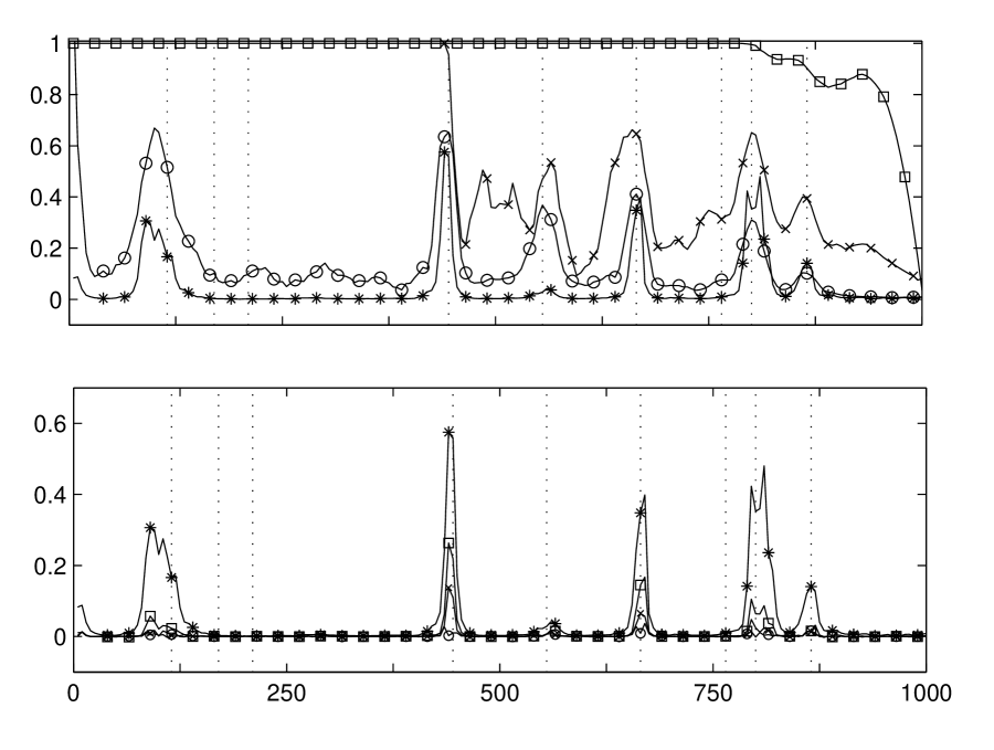
Figure 1: Example 1. Sample lag-$1$ autocorrelation for each of the discrete trajectory components $\left\{X_{n}(i),\>n=1,...,1000\right\}$ with (bottom) and without (top) backward sampling for various numbers of particles: $\square$: $N=10$; $\times$: $N=20$; $\bigcirc$: $N=50$; In both top and bottom $*$ is sample autocorrelation for standard one-at-a-time Gibbs. Vertical dashed lines are true locations of $X_{n}=1$.

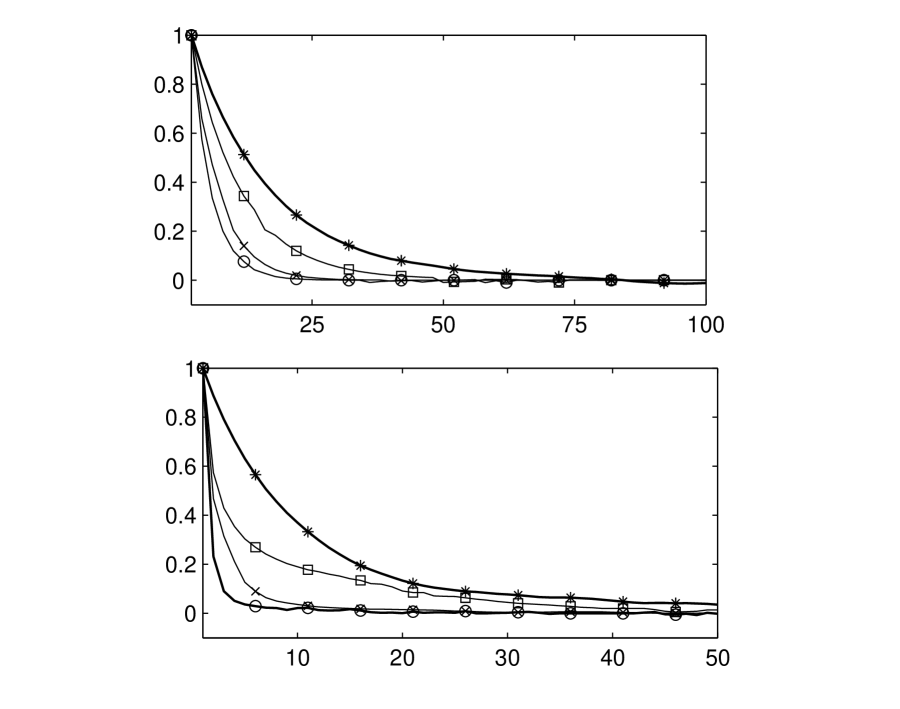
Figure 2: Example 1. Autocorrelation against lag for standard Gibbs sampler ($*$) and PG with backward sampling and various numbers of particles: $\square$: $N=10$; $\times$: $N=20$; $\bigcirc$: $N=50$. Top pane is for $\phi$ and bottom pane for $\sigma^{2}$.

5.1.2 Treatment of $P_{X}$

A common feature of SSSMs is that it is possible to analytically integrate out $P_{X}$ under Dirichlet priors for each of its rows and the autoregressive model with shifting level is no exception. It is natural to ask, even in the context of standard MCMC algorithms, whether it is beneficial to perform this integration analytically, or to treat $P_{X}$ as part of the sampling problem. To the authors’ knowledge, in the context of SSSMs this issue has not been treated in the literature.

Consider first the standard one-at-a-time Gibbs sampling case. The reader will recall from section 3.4 and Gerlach et al. (2000) that the algorithm involves sampling from

$$p_{\theta}\left(x_{n}|y_{1:T},x_{1:n-1},x_{n+1:T}\right)\propto p_{\theta}(y_{n}|y_{1:n-1},x_{1:n})p_{\theta}(x_{n}|x_{1:n-1},x_{n+1:T})p_{\theta}(y_{n+1:T}|y_{1:n},x_{1:T})$$ (26)

for each $n$. Conditionally on $P_{X}$, the process $\left\{X_{n}\right\}_{n\geq 1}$ is Markov and so in the above display we have the simplification $p_{\theta}(x_{n}|x_{1:n-1},x_{n+1:T})=p_{\theta}(x_{n}|x_{n-1},x_{n+1})$. Conversely, when $P_{X}$ is integrated out, in which case the parameter reduces to $\theta=[\phi\;\sigma^{2}]$, the process $\left\{X_{n}\right\}_{n\geq 1}$ is not Markov and the former simplification is not applicable. Thus, in terms of the correlation structure of the Markov chains generated by the corresponding Gibbs samplers, there appears to be a trade-off between conditioning on $P_{X}$ and conditioning on components of the $\left\{X_{n}\right\}_{n\geq 1}$ process when drawing from distributions of the form (26). In terms of computational cost there is no significant difference: in the case that $P_{X}$ is integrated out analytically evaluation of $p_{\theta}(x_{n}|x_{1:n-1},x_{n+1:T})$ requires only state-transition count statistics which are cheap to compute and store.

Analogous remarks to those above hold for the PG algorithm. It involves computing $f_{\theta}(x_{n}|x_{1:n-1})$ in the conditional DPF step and $p_{\theta}(x_{n+1:T}|x_{1:n})$ in the backward sampling step and it is in these places that the same conditioning issues arise. In our numerical experiments for this model and others we were unable to establish that either incorporating $P_{X}$ into the sampling problem or integrating it out analytically lead to a significant advantage in terms of sample autocorrelation, both for the standard one-at-a-time Gibbs sampler and the PG algorithm (results not shown). It would be very interesting to study the theoretical properties underlying this issue in Gibbs sampling algorithms for SSSMs but such an investigation is well beyond the scope of this article.

We found more obvious effects in the context of the PMMH algorithm, which we now go on to discuss. In this case $f_{\theta}(x_{n}|x_{1:n-1})$ is computed as part of the DPF algorithm, which is where the same conditioning issues arise. A data record of length $T=1000$ was generated from the model with the same true parameter values as stated in the previous section. The same prior distributions were also employed. Central to the performance of the PMMH algorithm is the normalizing constant estimate $\widehat{p}_{\theta}(y_{1:T})$ computed using the DPF. When the variance of this estimate is large the PMMH algorithm performs poorly, exhibiting a high rejection rate - a characteristic shared with the standard PMCMC algorithms in Andrieu et al. (2010). We found that in the two cases (where $P_{X}$ was integrated out and where it was not), the DPF exhibited striking differences in the variance of this estimate. The parameter $\theta$ was set to its true value and the DPF was run $1000$ times on the simulated data set. Figure 4 shows the sample variance of $\log\widehat{p}_{\theta}(y_{1:n})$ as a function of $n$. The bottom pane corresponds to the case in which $P_{X}$ is integrated out analytically. In this case the sample variance grows super-linearly with $n$. By contrast, as shown in the top pane, when conditioning on $P_{X}$ the variance grows far more slowly. Very similar results were obtained when conditioning on values of $P_{X}$ other than the truth. A step towards explaining this phenomenon is noting that integrating out $P_{X}$ destroys the ergodicity properties of the latent process $\left\{X_{n}\right\}$ conditional on $\theta$. For standard SMC algorithms it is now theoretically well understood that assumptions about the ergodicity properties of the latent process are central to establishing linear growth rates (with respect to $n$) for the error in normalizing constant-type estimates (Cérou et al., 2010). Our numerical results are consistent with the DPF having similar properties.

The variance of $\widehat{p}_{\theta}(y_{1:T})$ influences the acceptance rates of the corresponding two PMMH algorithms. Of course the trade-off is that when implementing a PMMH algorithm which incorporates $P_{X}$ into the sampling problem one has the added burden of designing proposal moves for $P_{X}$ and the contribution to the variability of the MH acceptance ratio from these proposals also influences the acceptance rate. In our experiments we found that an effective approach to making proposals for $P_{X}$ was to reparameterize the model in terms of the unnormalized components of each row of $P_{X}$, with the Dirichlet prior corresponding to gamma priors over these components. Proposals could then be made using log-Gaussian random walks (an analogous approach was advocated in the Jasra et al. (2005) in the context of static mixture models). In numerical experiments we adopted this approach with independent log-Gaussian random walk proposals made on each unnormalized component of $P_{X}$. After a couple of preliminary runs, the standard deviation of the increment in the log domain was set to $0.05$. A log-Gaussian random walk proposal with the same standard deviation was also used for the parameter $\sigma^{2}$ and a Gaussian random walk with standard deviation $0.1$ was used for $\phi$. For the case where $P_{X}$ is integrated out we used the same proposals as above for $\phi$ and $\sigma^{2}$. Figure 4 shows the PMMH acceptance rates as a function of the length of the data record. These results were obtained over $10^{5}$ iterations of the algorithms after a burn-in of $10^{4}$. The results show that the acceptance rate drops much more rapidly in the case that $P_{X}$ is integrated out. However, we cannot conclude that the PMMH algorithm is always more efficient when $P_{X}$ is incorporated into the sampling problem as the overall efficiency naturally depends on the particular choice of proposal mechanism for $P_{X}$. Our numerical results do indicate that even using a fairly simple proposal mechanism for $P_{X}$ one can obtain acceptance rates which are superior to those in the case that $P_{X}$ is integrated out analytically and the autocorrelation plots in Figure 5 show that this is carried over to lower sample autocorrelation for the parameters $\phi$ and $\sigma^{2}$.

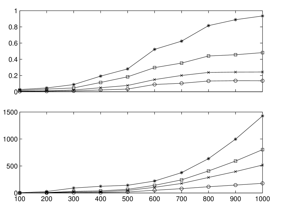
Figure 3: Example 1. Sample variance of $\log\widehat{p}_{\theta}(y_{1:n})$ for fixed $\theta$ as a function of $n$ for various numbers of particles: $*$: $N=10$; $\square$: $N=50$; $\times$: $N=100$; $\bigcirc$: $N=200$. Top pane is conditional on the true value of $P_{X}$ and bottom pane is with $P_{X}$ integrated out.

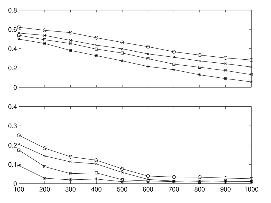
Figure 4: Example 1. PMMH acceptance rate as function of data record length for various numbers of particles: blue: $N=10$, green: $N=50$, red: $N=100$, black: $N=200$. Top pane is PMMH making proposals for $P_{X}$ and bottom pane is with $P_{X}$ integrated out.

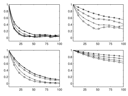
Figure 5: Example 1. Sample autocorrelation against lag for various numbers of particles, $*$: $N=10$; $\square$: $N=50$, $\times$: $N=100$; $\bigcirc$: $N=200$. Left column is PMMH with $P_{X}$ sampled and right column is with $P_{X}$ integrated out analytically. Top plots are for $\phi$ and bottom plots are for $\sigma^{2}$.

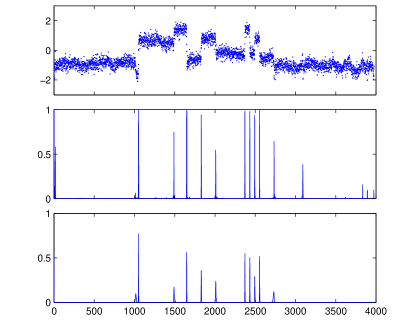
Figure 6: Example 2. Top: well-log data. Middle and bottom panes are estimated $p(X_{n}=2|y_{1:T})$ from respectively the standard Gibbs and PG samplers.

5.2 Example 2: Multiple change-point model with dependence between segments.

There is an extensive literature on statistical time series analysis based on multiple change-point models. In such models it is often assumed that given the position of a change-point, the data after that change-point are conditionally independent of those before, see for example Barry and Hartigan (1993); Fearnhead and Liu (2007), amongst many others. This modelling assumption may be restrictive in some circumstances. A natural way to relax it is via a SSSM, which allows the notion of change-points to be introduced whilst allowing potentially complex dependence structures across segments of the data.

We consider a multiple-change point model in which observations arise from a latent process which is piece-wise linear. Changes in the latent process are of two varieties: those in which there is a discontinuity in the latent trajectory and its gradient and those in which there is a discontinuity only in the gradient. More specifically, we have $\mathcal{X}=\{0,1,2\}$ and we assume that $\left\{X_{n}\right\}$ is Markov with unknown transition matrix $P_{X}.$ The observations $\left\{Y_{n}\right\}$ are real-valued, as are the latent trajectory $\left\{\mu_{n}\right\}$ and its gradient $\left\{\dot{\mu}_{n}\right\}$. In state-space form we have

$$Z_{n}=\left[\begin{array}[]{c}\mu_{n}\\ \dot{\mu}_{n}\end{array}\right],\quad A_{\theta}(0)=\left[\begin{array}[]{cc}1&\Delta\\ 0&1\end{array}\right],\quad A_{\theta}(1)=\left[\begin{array}[]{cc}1&\Delta\\ 0&0\end{array}\right],\quad A_{\theta}(2)=\left[\begin{array}[]{cc}0&0\\ 0&0\end{array}\right],$$

$$B_{\theta}(0)=\left[\begin{array}[]{cc}0&0\\ 0&0\end{array}\right],\quad B_{\theta}(1)=\left[\begin{array}[]{cc}0&0\\ 0&\sigma_{\mu,1}\end{array}\right],\quad B_{\theta}(2)=\left[\begin{array}[]{cc}\sigma_{\mu,0}&0\\ 0&\sigma_{\mu,1}\end{array}\right],$$

$$C_{\theta}(x_{n})=\left[\begin{array}[]{cc}1&0\end{array}\right],\quad D_{\theta}(x_{n})=\sigma_{Y},\quad F_{\theta}(x_{n})=G_{\theta}(x_{n})=0,\quad\forall x_{n}.$$

Here $\Delta$ is a fixed time incremement and the unknown parameters are $\theta=[\sigma_{Y}^{2}\;\sigma_{\mu,0}^{2}\;\sigma_{\mu,1}^{2}\;P_{X}]$. We apply this model to the analysis of well-log data: measurements of the nuclear resonance of underground rocks, as studied originally in O Ruanaidh and Fitzgerald (1996). Observations arise from a drill bit which passes down through layers of rock over time and each datum is a measurement of the resonance of the rock through which the bit is passing at that time. The aim is to identify segments in the data, each corresponding to a stratum of a single type of rock. The data set we analyse was treated in Fearnhead and Clifford (2003); Fearnhead and Liu (2007, 2010) under a variety of models, but in all these cases the static parameters of the models were assumed known. In Fearnhead and Liu (2010) a change-point model with dependence across segments was employed and its advantages in terms of avoiding spurious detection of change-points was demonstrated. We are interested in similar analysis, but without assuming fixed values for the static parameters of the model. As in Fearnhead and Clifford (2003); Fearnhead and Liu (2007, 2010) a few extreme outliers were removed from the data set manually resulting in $3975$ data points.

Flat Dirichlet priors were set on each row of $P_{X}$. Independent inverse gamma $(2,3)$ priors were placed over $\sigma_{Y}^{2}$, $\sigma_{\mu,0}^{2}$ and $\sigma_{\mu,1}^{2}$. In our experiments, inference was found to be insensitive to choice of parameters for these inverse gamma priors (not shown). For the initial distribution over $Z_{0}$ we set a relatively diffuse, zero mean Gaussian prior with diagonal covariance components $100$ and $100$, corresponding to $\mu_{0}$ and $\dot{\mu}_{0}$ respectively. We set $\Delta=0.1$. The standard Gibbs sampler was run for $2\times 10^{6}$ iterations and PG sampler with $N=50$ for $4\times 10^{4}$ iterations so as to equate computational cost. Histograms of sample output for $\sigma_{Y}^{2}$, $\sigma_{\mu,0}^{2}$ and $\sigma_{\mu,1}^{2}$ are shown in Figure 7. These results indicate that despite the long run the standard Gibbs sampler has not converged: most noticeably in the case of the histograms for $\sigma_{\mu,1}^{2}$, it appears not to have explored the support as thoroughly as the PG sampler and has become stuck in a mode of the distribution. The difference in performance is even more striking when considering the corresponding estimated posterior probabilities for the latent switching process. Figure 6 shows the estimated marginal posterior probabilities of each $X_{n}$ being in state $2$ (recall this state corresponds to a discontinuity in the latent process $\left\{\mu_{n}\right\}$ and its gradient) for each time step of the data record. Due to the lack of full exploration of the parameter space, the results for the standard Gibbs sampler show erroneously high posterior probabilities that each $X_{n}$ is in state 2. We can conclude that for the same computational cost the performance of the PG sampler is superior.

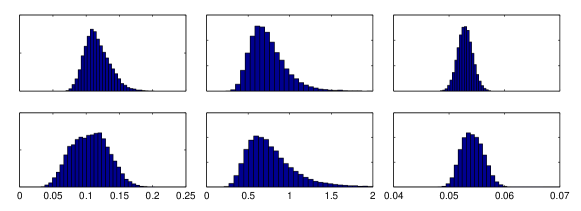
Figure 7: Example 2. Histograms estimates of posterior marginals. Top row: standard Gibbs sampler. Bottom row: PG sampler. Columns from left to right are $\sigma_{\mu,1}^{2}$, $\sigma_{\mu,0}^{2}$ and $\sigma_{Y}^{2}$.

5.3 Example 3: Exchange Rate Model

The following model was investigated in Engle and Kim (1999); Frühwirth-Schnatter (2006), where it was used to analyze economic data. The model consists of a latent random walk component observed in auto-regressive noise, where the variance of the observation noise innovations can switch between different values. In Engle and Kim (1999), this model was advocated to reflect the heteroscedasticity evident in the price index adjusted U.S./U.K. exchange rate during the late 19th and 20th centuries. The data consist of $1322$ monthly log exchange rate values. We consider the case treated in Frühwirth-Schnatter (2006) where the auto-regressive noise process is of order $2$ and there are $4$ switching states. In this model, $\mathcal{X}=\{1,2,3,4\}$ and the discrete latent process $\{X_{n}\}$ is a Markov chain with transition matrix $P_{X}$. The observations $\{Y_{n}\}$ are log-exchange rate values. The latent process $\left\{\mu_{n}\right\}$ is a random walk and we denote by $\left\{\eta_{n}\right\}$ the auto-regressive noise process:

$$Y_{n} =\mu_{n}+\eta_{n},$$

$$\mu_{n} =\mu_{n-1}+\sigma_{\mu}V_{n,1}$$

$$\eta_{n} =a_{1}\eta_{n-1}+a_{2}\eta_{n-2}+\sigma_{\eta,X_{n}}V_{n,2}$$

where $\{V_{n,1}\}$ and $\{V_{n,2}\}$ are i.i.d. $\mathcal{N}(0,1)$ noise sequences. In state-space form we then have

$$Z_{n}=\left[\begin{array}[]{c}\mu_{n}\\ \eta_{n}\\ \eta_{n-1}\end{array}\right],\quad A_{\theta}(x_{n})=\left[\begin{array}[]{ccl}1&0&0\\ 0&a_{1}&a_{2}\\ 0&1&0\end{array}\right],\quad B_{\theta}(x_{n})=\left[\begin{array}[]{ccl}\sigma_{\mu}&0&0\\ 0&\sigma_{\eta,x_{n}}&0\\ 0&0&0\end{array}\right],$$

$$C_{\theta}(x_{n})=\left[\begin{array}[]{ccl}1&1&0\end{array}\right],\quad D_{\theta}(x_{n})=F_{\theta}(x_{n})=G_{\theta}(x_{n})=0,\quad\forall x_{n}.$$

The unknown parameters of the model are $\theta=[\sigma_{\mu,}^{2}\;\sigma_{\eta,1}^{2}\;\sigma_{\eta,2}^{2}\;\sigma_{\eta,3}^{2}\;\sigma_{\eta,4}^{2}\;a_{1}\;a_{2}\;P_{X}]$. Under symmetric priors the labeling of the discrete states is not identifiable. We consider the same prior distributions on the parameters and initial conditions on $Z_{0}$ as in Frühwirth-Schnatter (2006) and we refer to the latter for full details, including a stability constraint on the auto-regressive coefficients $(a_{1,}a_{2})$. The only difference is that we do not impose an identifiability constraint a priori on $\sigma_{\eta,1}^{2},\sigma_{\eta,2}^{2},\sigma_{\eta,3}^{2},\sigma_{\eta,4}^{2}$, but instead target the unidentified model and impose the ordering $\sigma_{\eta,1}^{2}<\sigma_{\eta,2}^{2}<\sigma_{\eta,3}^{2}<\sigma_{\eta,4}^{2}$ after sampling (see Frühwirth-Schnatter (2001); Jasra et al. (2005) and references therein for various approaches to drawing inference in models with unidentifiable state labels).

We implemented an algorithm for this model with $P_{X}$ incorporated into the sampling. Each iteration of the algorithm consisted of a sequence of two PMMH updates. The first holding $P_{X}$ and $\sigma_{\eta,1}^{2},\sigma_{\eta,2}^{2},\sigma_{\eta,3}^{2},\sigma_{\eta,4}^{2}$ constant and the second holding $(a_{1,}a_{2})$ and $\sigma_{\mu}^{2}$ constant (using standard arguments for Metropolis-within-Gibbs algorithms and Theorem 1 it is straightforward to show this sequence of updates is invariant with respect to the extended target distribution). After a couple of preliminary runs the following proposals were selected. A symmetric random walk proposal of standard deviation of $0.001$ was used for $(a_{1,}a_{2})$ and for $\sigma_{\mu}^{2}$ a log-Gaussian random walk with log-domain standard deviation of $0.01$. We used a mixture of log-Gaussian random walks for the unnormalised components of $P_{X}$ and $\sigma_{\eta,1}^{2},\sigma_{\eta,2}^{2},\sigma_{\eta,3}^{2},\sigma_{\eta,4}^{2}$. For each individual parameter, the mixture had two components, the first with weight $0.9$ and standard deviation $0.05$ in the log domain and the second with weight $0.1$ and standard deviation $1$ in the log domain. With these settings and $N=200$ we achieved an overall acceptance rate of $0.2$. This is a reasonable rate given the mixture proposals. The algorithm was run for $2\times 10^{5}$ iterations after an initial burn-in of $10^{4}$. Inferential summaries are presented in Figures 8-10. We note that there are some differences between the results we obtained and those from Frühwirth-Schnatter (2006), where a standard Gibbs sampler was applied. We conjecture that the latter had not fully explored the support of the posterior distribution. Noticeable differences are that the posterior marginal for $\sigma_{\eta,1}^{2}$ we obtain is more diffuse than that reported in Frühwirth-Schnatter (2006) and we obtain a much flatter trajectory in the posterior estimates of $\{\mu_{n}\}$ in Figure 10. Another significant difference is that we obtain concentration of the marginal posterior over the auto-regressive coefficients $(a_{1},a_{2})$ in a different region than that reported in Frühwirth-Schnatter (2006). Using other proposals for $(a_{1},a_{2})$ we were not able to find another major mode. Furthermore the posterior marginal for $\sigma_{\mu}^{2}$ we obtained is concentrated on lower values. Overall, we feel that the ability to integrate out approximately the latent variables makes the PMMH algorithm a powerful tool: as these results demonstrate it gives us the chance to explore regions of posterior support which Gibbs sampling algorithms may struggle to find.

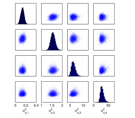
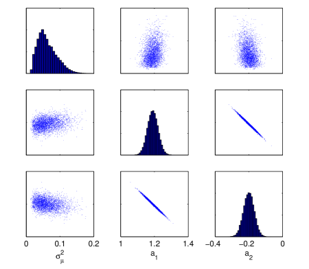
Figure 8: Example 3. Histogram estimates of posterior marginals and scatter plots of pairwise marginals for the exchange rate model.

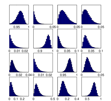
Figure 9: Example 3. Histogram estimates of marginal posterior distributions for entries of the state transition matrix $P_{X}$. Panes are arranged as per the transition matrix itself.

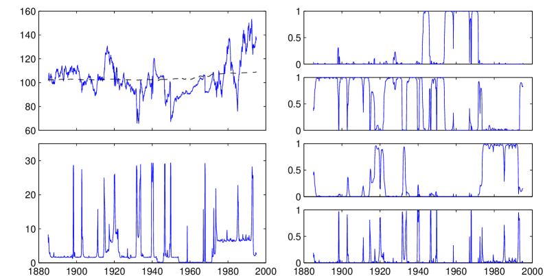
Figure 10: Example 3. Top left: data (solid) and $\mathbb{E}\left[\left.\mu_{n}\right|y_{1:T}\right]$ (dashed). Bottom left: $\mathbb{E}\left[\left.\sigma_{\eta,X_{n}}^{2}\right|y_{1:T}\right]$. Right: estimated posterior probabilities $p(X_{n}=j|y_{1:T})$ for, top to bottom, $j=1,2,3,4$.

6 Discussion and extensions

In this article, we have proposed new PMCMC algorithms relying on the efficient DPF algorithm to perform Bayesian inference in SSSM. We have shown experimentally that these generic discrete PMCMC algorithms outperform current state-of-the-art MCMC techniques for a given computational complexity. Moreover the DPF can be easily parallelised so further substantial improvements could be obtained.

There are various possible extensions to this work. First, we have restricted ourselves to SSSM but the DPF can be applied to any model where the latent process is discrete-valued. This includes for example Dirichlet process mixtures (Fearnhead, 2004) and the infinite hidden Markov model introduced in Teh et al. (2006). Compared to the SSSM framework, the differences are that, in these scenarios, $X_{n}$ takes values in a set whose cardinality increases over time and computations required to evaluate the importance weights are not performed using the Kalman filter. However, the discrete PMCMC methodology discussed here can be straightforwardly extended to these cases. Second, it would be possible to extend the DPF and the associated discrete PMCMC methodology by using look-ahead techniques. In a look-ahead strategy with an integer lag $L$, we resample trajectories at time $n$ by considering the weights proportional to $p_{\theta}\left(x_{1:n}|y_{1:n+L}\right)$ instead of $p_{\theta}\left(x_{1:n}|y_{1:n}\right)$ for the standard DPF. This is obviously more expensive than the DPF as computation of the weights involves summing over $x_{n+1:L}$ for each particle, but this might be of interest in scenarios where future observations are very informative about $X_{n}$.

Appendix A Kalman Filter

Conditional upon $X_{1:T}=x_{1:T}$, Eq. (2)-(3) defines a linear Gaussian state-space model. The Kalman filter allows us to compute recursively in time $p_{\theta}\left(\left.z_{n}\right|y_{1:n-1},x_{1:n}\right)=\mathcal{N}\left(z_{n};m_{\left.n\right|n-1}^{z,\theta}\left(x_{1:n}\right),\Sigma_{\left.n\right|n-1}^{z,\theta}\left(x_{1:n}\right)\right)$, $p_{\theta}\left(\left.z_{n}\right|y_{1:n},x_{1:n}\right)=\mathcal{N}\left(z_{n};m_{\left.n\right|n}^{z,\theta}\left(x_{1:n}\right),\Sigma_{\left.n\right|n}^{z,\theta}\left(x_{1:n}\right)\right)$ and the predictive density
$g_{\theta}\left(\left.y_{n}\right|y_{1:n-1},x_{1:n}\right)=\mathcal{N}\left(y_{n};m_{\left.n\right|n-1}^{y,\theta}\left(x_{1:n}\right),\Sigma_{\left.n\right|n-1}^{y,\theta}\left(x_{1:n}\right)\right)$. For $n\geq 1$ these statistics are computed using the following recursion initialized with $m_{\left.0\right|0}^{z}=m_{0},$ $\Sigma_{\left.0\right|0}^{z}=\Sigma_{0}$

$$m_{\left.n\right|n-1}^{z,\theta}\left(x_{1:n}\right) =A_{\theta}(x_{n})m_{\left.n-1\right|n-1}^{z}\left(x_{1:n-1}\right)+F_{\theta}(x_{n})u_{n},\text{ }$$

$$\Sigma_{\left.n\right|n-1}^{z,\theta}\left(x_{1:n}\right) =A_{\theta}(x_{n})\Sigma_{\left.n-1\right|n-1}^{z}A_{\theta}^{\text{T}}(x_{n})+B_{\theta}(x_{n})B_{\theta}^{\text{T}}(x_{n}),$$

$$m_{\left.n\right|n-1}^{y,\theta}\left(x_{1:n}\right) =C_{\theta}(x_{n})m_{\left.n\right|n-1}^{z,\theta}\left(x_{1:n}\right)+G_{\theta}(x_{n})u_{n},$$

$$\Sigma_{\left.n\right|n-1}^{y,\theta}\left(x_{1:n}\right) =C_{\theta}(x_{n})\Sigma_{\left.n\right|n-1}^{z,\theta}\left(x_{1:n}\right)C_{\theta}^{\text{T}}(x_{n})+D_{\theta}(x_{n})D_{\theta}^{\text{T}}(x_{n}),$$

$$m_{\left.n\right|n}^{z,\theta}\left(x_{1:n}\right) =m_{\left.n\right|n-1}^{z,\theta}\left(x_{1:n}\right)+\Sigma_{\left.n\right|n-1}^{z,\theta}\left(x_{1:n}\right)C_{\theta}^{\text{T}}(x_{n})\left[\Sigma_{\left.n\right|n-1}^{y,\theta}\left(x_{1:n}\right)\right]^{-1}\left(y_{n}-m_{\left.n\right|n-1}^{y,\theta}\left(x_{1:n}\right)\right),$$

$$\Sigma_{\left.n\right|n}^{z,\theta}\left(x_{1:n}\right) =\Sigma_{\left.n\right|n-1}^{z,\theta}\left(x_{1:n}\right)-\Sigma_{\left.n\right|n-1}^{z,\theta}\left(x_{1:n}\right)C_{\theta}^{\text{T}}(x_{n})\left[\Sigma_{\left.n\right|n-1}^{y,\theta}\left(x_{1:n}\right)\right]^{-1}C_{\theta}\left(x_{n}\right)\Sigma_{\left.n\right|n-1}^{z,\theta}\left(x_{1:n}\right).$$

Appendix B Backward Sampling

A key component of the backward sampling algorithm is the evaluation of the backward weight

$$V_{n}^{\theta}\left(x_{1:n}\left|x_{n+1:T}^{\prime}\right.\right)\propto W_{n}^{\theta}(x_{1:n})p_{\theta}(x_{n+1:T}^{\prime}|x_{1:n})p_{\theta}(y_{n+1:T}|y_{1:n},x_{1:n},x_{n+1:T}^{\prime})$$

for each candidate sub-trajectory $x_{1:n}$ and where $x_{n+1:T}^{\prime}$ is the complementing sub-trajectory which has been obtained from previous steps of the backward sampling procedure. Central to the computation of this weight is the identity

$$p_{\theta}(y_{n+1:T}|y_{1:n},x_{1:n},x_{n+1:T}^{\prime})=\int p_{\theta}(y_{n+1:T}|z_{n},x_{n+1:T}^{\prime})p_{\theta}(z_{n}|x_{1:n},y_{1:n})dz_{n},$$ (27)

where $p_{\theta}(z_{n}|x_{1:n},y_{1:n})$ is the Gaussian conditional filtering density associated with the sub-trajectory $x_{1:n}$ and is specified by its mean vector $m_{\left.n\right|n}^{z,\theta}\left(x_{1:n}\right)$ and co-variance matrix $\Sigma_{\left.n\right|n}^{z,\theta}\left(x_{1:n}\right)$. In order to compute (27) (at least up to a constant of proportionality) it is necessary to obtain the coefficients of $z_{n}$ in $p_{\theta}(y_{n+1:T}|z_{n},x_{n+1:T}^{\prime})$. The latter can be expressed as

$$p_{\theta}(y_{n+1:T}|z_{n},x_{n+1:T}^{\prime})\propto\exp\left[-\frac{1}{2}\left(z_{n}^{T}\Xi_{n}z_{n}-2\mu_{n}^{T}z_{n}\right)\right]$$

where $\Xi_{n}$ and $\mu_{n}$ are respectively a matrix and vector of appropriate dimension, both depending on $x_{n+1:T}^{\prime}$, $y_{n+1:T}$ and $\theta$. In the following this dependence is suppressed from the notation for convenience. For ease of presentation we use the similarly abusive conventions in writing $m_{n}=m_{\left.n\right|n}^{z,\theta}\left(x_{1:n}\right)$, $\Sigma_{n}=\Sigma_{\left.n\right|n}^{z,\theta}\left(x_{1:n}\right)$, $A_{n}=A_{\theta}(x_{n})$, $B_{n}=\left[B_{\theta}(x_{n})\;\;0_{z\times w}\right]$, $C_{n}=C_{\theta}(x_{n})$, $D_{n}=\left[0_{y\times v}\;\;D_{\theta}(x_{n})\right],$ $F_{n}=F_{\theta}(x_{n})$, $G_{n}=G_{\theta}(x_{n})$. Then let $\Upsilon_{n}$ be a matrix satisfying $\Sigma_{\left.n\right|n}^{z,\theta}\left(x_{1:n}\right)=\Upsilon_{n}\Upsilon_{n}^{T}$. We have

$$p_{\theta}(y_{n+1:T}|y_{1:n},x_{1:n},x_{n+1:T}^{\prime})$$

$$\propto\exp\left(-\frac{1}{2}\left[m_{n}^{T}\Xi_{n}m_{n}-2\mu_{n}^{T}m_{n}-\left(\mu_{n}-\Xi_{n}m_{n}\right)^{T}\Upsilon_{n}\left(\Upsilon_{n}\Xi_{n}\Upsilon_{n}+I\right)^{-1}\Upsilon_{n}^{T}\left(\mu_{n}-\Xi_{n}m_{n}\right)\right]\right)$$

$$\quad\times\left|\Upsilon_{n}^{T}\Xi_{n}\Upsilon_{n}+I\right|^{-1/2}.$$ (28)

where $I$ is the identity matrix of appropriate dimension. We now specify equations for updating $(\mu_{n},\Xi_{n})$, which are given without proof of validity: they are a direct application of Lemmata 1 and 2 in Gerlach et al. (2000). As in Gerlach et al. (2000), for simplicity we present recursions only for the case in which the observations are scalar-valued, but they can readily be extended to the vector-valued case. Let

$$r_{n+1}= \left(C_{n+1}B_{n+1}+D_{n+1}\right)\left(C_{n+1}B_{n+1}+D_{n+1}\right)^{T},$$

$$\Phi_{n+1}= B_{n+1}\left(B_{n+1}^{T}C_{n+1}^{T}+D_{n+1}^{T}\right)/r_{n+1},$$

$$\Lambda_{n+1}= \left(1-\Phi_{n+1}C_{n+1}^{T}\right)A_{n+1},$$

$$a_{n+1}= \left(1-\Phi_{n+1}C_{n+1}^{T}\right)F_{n+1}u_{n+1}-\Phi_{n+1}G_{n+1}u_{n+1},$$

and let $\Gamma_{n+1}$ be a matrix which satisfies

$$\Gamma_{n+1}\Gamma_{n+1}^{T}=B_{n+1}\left(I-\frac{1}{r_{n+1}}\left(B_{n+1}^{T}C_{n+1}^{T}+D_{n+1}^{T}\right)\left(B_{n+1}^{T}C_{n+1}^{T}+D_{n+1}^{T}\right)^{T}\right)B_{n+1}^{T}.$$

The recursion for $(\mu_{n},\Xi_{n})$ is then given by

• Set $\Xi_{T}=0$, $\mu_{T}=0$.

• For $n=T-1,...,1$

  $$M_{n+1} = \Gamma_{n+1}^{T}\Xi_{n+1}\Gamma_{n+1}+I,$$

  $$\Xi_{n} = \Lambda_{n+1}^{T}\left(\Xi_{n+1}-\Xi_{n+1}\Gamma_{n+1}M_{n+1}^{-1}\Gamma_{n+1}^{T}\Xi_{n+1}\right)\Lambda_{n+1}+A_{n+1}^{T}C_{n+1}^{T}C_{n+1}A_{n+1}\frac{1}{r_{n+1}},$$

  $$\mu_{n} = \Lambda_{n+1}^{T}\left(I-\Xi_{n+1}\Gamma_{n+1}M_{n+1}^{-1}\Gamma_{n+1}^{T}\right)\left(\mu_{n+1}-\Xi_{n+1}\left(a_{n+1}+\Phi_{n+1}y_{n+1}\right)\right)$$

  $$+A_{n+1}^{T}C_{n+1}^{T}\left(y_{n+1}-G_{n+1}u_{n+1}-C_{n+1}F_{n+1}u_{n+1}\right)\frac{1}{r_{n+1}}.$$

Appendix C Proofs

Proof of Theorem 1. We obtain from Eq. (22)-(23)-(24) that on the event $x_{1:T}\in\mathbf{S}_{T}$,

$$\frac{\pi_{\theta}^{N}(x_{1:T},\mathbf{s}_{1},\mathbf{s}_{2},...,\mathbf{s}_{T})}{w_{T}^{\theta}\left(x_{1:T}\right)\text{ }\psi_{\theta}^{N}\left(\mathbf{s}_{1},\mathbf{s}_{2},...,\mathbf{s}_{T}\right)} =\frac{p_{\theta}(\left.x_{1:T}\right|y_{1:T})\left\{\prod_{n=2}^{T}\mathbb{I}[x_{1:n}\in\mathbf{s}_{n}]\right\}}{w_{T}^{\theta}\left(x_{1:T}\right)\prod_{n=2}^{T}r_{n}^{N}(x_{1:n}\in\mathbf{s}_{n}|\mathbf{w}_{n-1}^{\theta})}$$

$$=\frac{p_{\theta}(\left.x_{1:T}\right|y_{1:T})\left\{\prod_{n=2}^{T}\mathbb{I}[x_{1:n}\in\mathbf{s}_{n}]\right\}}{w_{T}^{\theta}\left(x_{1:T}\right)\prod_{n=1}^{T-1}\left(1\wedge C_{n}w_{n}^{\theta}\left(x_{1:n}\right)\right)}.$$

It follows from Eq. (10)-(11) that on the event $x_{1:T}\in\mathbf{S}_{T}$ the normalized weight can be expanded as follows

$$w_{T}^{\theta}\left(x_{1:T}\right) =\nu_{\theta}(x_{1})g_{\theta}(y_{1}|x_{1})\prod_{n=2}^{T}f_{\theta}(x_{n}|x_{1:n-1})g_{\theta}(y_{n}|y_{1:n-1},x_{1:n})$$

$$\times\prod_{n=1}^{T-1}\frac{1}{1\wedge C_{n}w_{n}^{\theta}\left(x_{1:n}\right)}\text{ }\prod_{n=1}^{T}\left\{\sum_{x_{1:n}^{\prime}\in\mathbf{s}_{n}}\overline{w}_{n}^{\theta}\left(x_{1:n}^{\prime}\right)\right\}^{-1}$$ (29)

Hence, using Eq. (12)-(13), we obtain

$$\frac{\pi_{\theta}^{N}(x_{1:T},\mathbf{s}_{1},\mathbf{s}_{2},...,\mathbf{s}_{T})}{w_{T}^{\theta}\left(x_{1:T}\right)\text{ }\psi_{\theta}^{N}\left(\mathbf{s}_{1},\mathbf{s}_{2},...,\mathbf{s}_{T}\right)}=\frac{\widehat{p}_{\theta}\left(y_{1:T}\right)}{p_{\theta}\left(y_{1:T}\right)}.$$ (30)

From (30), we can now easily establish that an MH sampler of target density (24) and proposal density (25) admits indeed Eq. (17) as MH ratio and the first part of the theorem follows. The second part of the proof is a direct consequence of Theorem 1 in Andrieu and Roberts (2006) and (A(A1)). $\blacksquare$

Proof of Proposition 1. First note that, from Eq. (24) and Eq. (29), for $\theta,\mathbf{s}_{1},\mathbf{s}_{2},...,\mathbf{s}_{T}$ in the support of $\pi^{N}(\theta,\mathbf{s}_{1},\mathbf{s}_{2},...,\mathbf{s}_{T})$,

$$\pi^{N}(x_{1:T}|\theta,\mathbf{s}_{1},\mathbf{s}_{2},...,\mathbf{s}_{T}) \propto p_{\theta}(\left.x_{1:T}\right|y_{1:T})\left\{\prod_{n=2}^{T}\mathbb{I}[x_{1:n}\in\mathbf{s}_{n}]\right\}\frac{\psi_{\theta}^{N}(\mathbf{s}_{1},\mathbf{s}_{2},...,\mathbf{s}_{T})}{\prod_{n=2}^{T}r_{n}^{N}(x_{1:n}\in\mathbf{s}_{n}|\mathbf{w}_{n-1}^{\theta})}$$

$$\propto \nu_{\theta}(x_{1})g_{\theta}(y_{1}|x_{1})\prod_{n=2}^{T}f_{\theta}(x_{n}|x_{1:n-1})g_{\theta}(y_{n}|y_{1:n-1},x_{1:n})$$

$$\times\left\{\prod_{n=2}^{T}\mathbb{I}[x_{1:n}\in\mathbf{s}_{n}]\right\}\prod_{n=1}^{T-1}\frac{1}{1\wedge c_{n}w_{n}^{\theta}\left(x_{1:n}\right)}$$

$$\propto w_{T}^{\theta}(x_{1:T}).$$

Furthermore, for $1\leq n\leq T-1$,

$$\pi^{N}(x_{1:n}|\theta,x_{n+1:T},\mathbf{s}_{1},\mathbf{s}_{2},...,\mathbf{s}_{n}) \propto p_{\theta}(x_{1:T}|y_{1:T})\left\{\prod_{k=2}^{n}\mathbb{I}[x_{1:k}\in\mathbf{s}_{k}]\right\}\frac{\psi_{\theta}^{N}(\mathbf{s}_{1},\mathbf{s}_{2},...,\mathbf{s}_{n})}{\prod_{k=2}^{n}r_{k}^{N}(x_{1:k}\in\mathbf{s}_{k}|\mathbf{w}_{k-1}^{\theta})}$$ (32)

$$\propto \frac{p_{\theta}(x_{1:n}|y_{1:n})}{\prod_{k=2}^{n}r_{k}^{N}(x_{1:k}\in\mathbf{s}_{k}|\mathbf{w}_{k-1}^{\theta})}p_{\theta}(x_{n+1:T}|x_{1:n})p_{\theta}(y_{n+1:T}|y_{1:n},x_{1:T})$$

$$\times\left\{\prod_{k=2}^{n}\mathbb{I}[x_{1:k}\in\mathbf{s}_{k}]\right\}$$

$$\propto w_{n}^{\theta}(x_{1:n})p_{\theta}(x_{n+1:T}|x_{1:n})p_{\theta}(y_{n+1:T}|y_{1:n},x_{1:T})$$

$$\propto v_{n}^{\theta}\left(x_{1:n}\left|x_{n+1:T}\right.\right),$$

where for the third proportionality we have used (19)-(20) and an expansion of $W_{n}^{\theta}(x_{1:n})$ which is the direct analogue of (29) but for final time index $n$.

To establish the assertion of the proposition we use an inductive argument over the iterations of the backward sampling algorithm (indexed by $n=T,T-1,...,1$). The inductive hypothesis is that for some index $n$ satisfying $1<m<n<T$ of the backward sampling procedure, $\left(X_{1:T}^{\prime},\mathbf{S}_{1},\mathbf{S}_{2},...,\mathbf{S}_{n}\right)$ obtained immediately after sampling from the backwards weights is distributed according to the marginal distribution $\sum_{\mathbf{s}_{n+1}}...\sum_{\mathbf{s}_{T}}\pi_{\theta}^{N}(x_{1:T},\mathbf{s}_{1},\mathbf{s}_{2},...,\mathbf{s}_{T})$. This implies $\left(X_{n:T}^{\prime},\mathbf{s}_{1},\mathbf{s}_{2},...,\mathbf{s}_{n-1}\right)$ is distributed according to $\sum_{x_{1:n-1}}\sum_{\mathbf{s}_{n}}...\sum_{\mathbf{s}_{T}}\pi_{\theta}^{N}(x_{1:T},\mathbf{s}_{1},\mathbf{s}_{2},...,\mathbf{s}_{T})$. Then at time step $n-1$, due to Eq. (32), $\left(X_{1:T}^{\prime},\mathbf{s}_{1},\mathbf{s}_{2},...,\mathbf{s}_{n-1}\right)$ obtained after sampling from the backward weights is distributed according to $\sum_{\mathbf{s}_{n}}...\sum_{\mathbf{s}_{T}}\pi_{\theta}^{N}(x_{1:T},\mathbf{s}_{1},\mathbf{s}_{2},...,\mathbf{s}_{T})$ and thus $X_{1:T}^{\prime}$ is distributed according to $\sum_{\mathbf{s}_{1}}...\sum_{\mathbf{s}_{T}}\pi_{\theta}^{N}(x_{1:T},\mathbf{s}_{1},\mathbf{s}_{2},...,\mathbf{s}_{T})=p_{\theta}(x_{1:T}|y_{1:T})$. Next note that, due to Eq. (C) the first step of the backward sampling procedure draws from $\pi_{\theta}^{N}(x_{1:T}|\mathbf{s}_{1},\mathbf{s}_{2},...,\mathbf{s}_{T})$. The proof is then complete under the assumption of the proposition. $\blacksquare$

Proof of Theorem 2. For part $1$, it is easy to check that steps $1-4$ of the PG algorithm define a collapsed Gibbs sampler targeting Eq. (24). This follows from Proposition 1 and the fact that the conditional DPF update, given a value of $\theta$ and $x_{1:T}$, is nothing but an algorithm sampling from

$$\left\{\prod_{n=2}^{T}\mathbb{I}[x_{1:n}\in\mathbf{s}_{n}]\right\}\frac{\psi_{\theta}^{N}(\mathbf{s}_{1},\mathbf{s}_{2},...,\mathbf{s}_{T})}{\prod_{n=2}^{T}r_{\theta}^{N}(x_{1:n}\in\mathbf{s}_{n}|\mathbf{w}_{n-1}^{\theta})}.$$

For part $2$, we focus on establishing irreducibility and aperiodicity of the transition probability of this algorithm. We denote by $\mathcal{L}_{G}$ the law of the Gibbs sampler to which assumption (A2) applies and $\mathcal{L}_{PG}^{N}$ the law of the PG sampler using $N$ particles.

For any set $U$ write $2^{U}$ for the power set of $U$ and let $\mathcal{B}(\Theta)$ denote a $\sigma$-algebra on $\Theta$. Let $A\times B\times C\in\mathcal{B}(\Theta)\times 2^{\mathcal{X}^{T}}\times\prod_{n=1}^{T}2^{\mathcal{P}(\mathcal{X}^{n})}$ be such that $\pi^{N}(\theta\in A,X_{1:T}\in B,\mathbf{S}_{1},...,\mathbf{S}_{T-1}\in C)>0$. It follows that $\pi(\left(\theta,X_{1:T}\right)\in A\times B)>0$ and then from irreducibility of the corresponding Gibbs sampler (Assumption (A2)) there exists a finite $j$ such that $\mathcal{L}_{G}(\left(\theta(j),X_{1:T}(j)\right)\in A\times B)>0$.

From the definition of the conditional DPF update, it is straightforward to check that, for any $\theta\in\Theta$, $N\geq 2$, given any $x_{1:T}$ and for any time step, any particle which has positive weight immediately before resampling has a positive probability of surviving that resampling step. Thus, by an inductive argument in $n$, any point in the support of $p_{\theta}(x_{1:T}|y_{1:T})$ has positive probability of being assigned a positive weight at time $T$. It then follows from the above arguments that $A\times B$ is marginally an accessible set of the PG sampler for the same $j$: i.e. $\mathcal{L}_{PG}^{N}(\left(\theta(j),X_{1:T}(j)\right)\in A\times B)>0$. Furthermore, as the conditional DPF update corresponds to drawing from the conditional of $\pi^{N}$ given $\theta$ and $X_{1:T}$,

$$\mathcal{L}_{PG}^{N}(\left(\theta(j+1),X_{1:T}(j+1),\mathbf{S}_{1}(j+1),...,\mathbf{S}_{T}(j+1)\right)\in A\times B\times C)>0$$

and irreducibility follows. Furthermore, aperiodicity of the PG sampler holds by contradiction: if the PG sampler were periodic, then the Gibbs sampler would be too; this violates Assumption A(A2).$\blacksquare$

References

- Andrieu et al. (2010) Andrieu, C., A. Doucet, and R. Holenstein (2010). Particle Markov chain Monte Carlo methods (with discussion). J. Roy. Stat. Soc. B 72, 269–342.
- Andrieu and Roberts (2006) Andrieu, C. and G. Roberts (2006). The pseudo-marginal approach for efficient computation. Annals Statist. 37, 697–725.
- Barembruch et al. (2009) Barembruch, S., A. Garivier, and E. Moulines (2009). On approximate maximum likelihood methods for blind identification: how to cope with the curse of dimensionality. IEEE Trans. Signal Proc. 57(11), 4247–4259.
- Barry and Hartigan (1993) Barry, D. and J. A. Hartigan (1993). A Bayesian analysis for change point problems. J. Am. Stat. Assoc. 88(421), 309–319.
- Billio and Monfort (1998) Billio, M. and A. Monfort (1998). Switching state space models: likelihood, filtering and smoothing. J. Stat. Planning Inf. 68, 65–103.
- Cappé et al. (2005) Cappé, O., E. Moulines, and T. Rydén (2005). Inference in Hidden Markov Models. New York: Springer-Verlag.
- Carpenter et al. (1999) Carpenter, J., P. Clifford, and P. Fearnhead (1999). An improved particle filter for non-linear problems. IEE Proc. F 146, 2–7.
- Carter and Kohn (1994) Carter, C. and R. Kohn (1994). On Gibbs sampling for state space models. Biometrika 81, 541–553.
- Carter and Kohn (1996) Carter, C. and R. Kohn (1996). Markov chain Monte Carlo in conditionally Gaussian state space models. Biometrika 83, 589–601.
- Cérou et al. (2010) Cérou, F., P. Del Moral, and A. Guyader (2010). A non asymptotic variance theorem for unnormalized Feynman-Kac particle models. Annales de l’Institut Henri Poincaré B. To appear.
- Chen and Liu (2000) Chen, R. and J. Liu (2000). Mixture Kalman filters. J. Roy. Stat. Soc. B 62, 493–508.
- Chib (1996) Chib, S. (1996). Calculating posterior distributions and modal estimates in Markov mixture models. J. Econometrics 75, 79–97.
- Costa et al. (2005) Costa, O., M. D. Fragoso, and R. Marques (2005). Discrete-Time Markovian Jump Linear Systems. Springer-Verlag.
- De Jong and Shephard (1995) De Jong, P. and N. Shephard (1995). The simulation smoother for time series models. Biometrika 82, 339–350.
- Del Moral (2004) Del Moral, P. (2004). Feynman-Kac Formulae: Genealogical and Interacting Particle Systems with Applications. New York: Springer-Verlag.
- Doucet et al. (2001) Doucet, A., J. de Freitas, and N. Gordon (Eds.) (2001). Sequential Monte Carlo Methods in Practice, New York. Sprigner-Verlag.
- Doucet et al. (2000) Doucet, A., S. Godsill, and C. Andrieu (2000). On sequential Monte Carlo sampling methods for Bayesian filtering. Statist. Comput. 10, 197–208.
- Doucet et al. (2001) Doucet, A., N. Gordon, and V. Krishnamurthy (2001). Particle filters for state estimation of jump Markov linear systems. IEEE Trans. Signal Proc. 49, 613–624.
- Durbin and Koopman (2002) Durbin, J. and S. Koopman (2002). A simple and efficient simulation smoother for state space time series analysis. Biometrika 89, 603–616.
- Engle and Kim (1999) Engle, C. and C.-J. Kim (1999). The long-run U.S./U.K. real exchange rate. J. Money, Credit and Banking 31, 335–356.
- Fearnhead (1998) Fearnhead, P. (1998). Sequential Monte Carlo methods in filter theory. D.Phil. thesis, Department of Statistics, University of Oxford.
- Fearnhead (2004) Fearnhead, P. (2004). Particle filters for mixture models with an unknown number of components. Statist. Comput. 14, 11–21.
- Fearnhead and Clifford (2003) Fearnhead, P. and P. Clifford (2003). Online inference for well-log data. J. Roy. Stat. Soc. B 65, 887–899.
- Fearnhead and Liu (2007) Fearnhead, P. and Z. Liu (2007). On-line inference for multiple changepoint problems. J. Roy. Statist. Soc. B 69, 589–605.
- Fearnhead and Liu (2010) Fearnhead, P. and Z. Liu (2010). Efficient bayesian analysis of multiple changepoint models with dependence across segments. Statist. Comput.. To appear.
- Flury and Shephard (2010) Flury, T. and N. Shephard (2010). Bayesian inference based only on simulated likelihood: particle filter analysis of dynamic economic models. Econometrics Theory. To appear.
- Fong et al. (2002) Fong, W., S. Godsill, A. Doucet, and M. West (2002). Monte Carlo smoothing with application to audio signal enhancement. IEEE Trans. Signal Proc. 50(2), 438–449.
- Frühwirth-Schnatter (1994) Frühwirth-Schnatter, S. (1994). Data augmentation and dynamic linear models. J. Time Series Analysis 15, 183–202.
- Frühwirth-Schnatter (2001) Frühwirth-Schnatter, S. (2001). Markov chain Monte Carlo estimation of classical and dynamic switching and mixture models. J. Amer. Statist. Assoc. 96(453), 194–209.
- Frühwirth-Schnatter (2006) Frühwirth-Schnatter, S. (2006). Finite Mixture and Markov Switching Models. New York: Springer-Verlag.
- Gerlach et al. (2000) Gerlach, R., C. K. Carter, and R. Kohn (2000). Efficient Bayesian inference for dynamic mixture models. J. Amer. Statist. Assoc. 95, 819–828.
- Giordani and Kohn (2008) Giordani, P. and R. Kohn (2008). Efficient Bayesian inference for multiple change-point and mixture innovation models. J. Business Economic Statist. 26, 66–77.
- Giordani et al. (2007) Giordani, P., R. Kohn, and D. van Dijk (2007). A unified approach to nonlinearity, structural change and outliers. J. Econometrics 137, 112–133.
- Hammer and Tjelmeland (2011) Hammer, H. and H. Tjelmeland (2011). Approximate forward-backward algorithm for a switching linear Gaussian model. Comput. Stat. and Dat. Anal.. To appear.
- Jasra et al. (2005) Jasra, A., C. C. Holmes, and S. D. A. (2005). Markov chain Monte Carlo methods and the label switching problem in Bayesian mixture modeling. Statist. Sci. 20(1), 50–67.
- Kim and Nelson (1999) Kim, C. and C. Nelson (1999). State-Space Models with Regime Switching: Classical and Gibbs-Sampling Approaches with Applications. MIT Press.
- Kitagawa (1996) Kitagawa, G. (1996). Monte Carlo filter and smoother for non-Gaussian nonlinear state space models. J. Comp. Graph. Statist. 5, 1–25.
- Lee et al. (2010) Lee, A., C. Yau, M. Giles, A. Doucet, and C. Holmes (2010). On the utility of graphics cards to perform massively parallel simulation of advanced Monte Carlo methods. J. Comp. Graph. Statist.. To appear.
- Liu (2001) Liu, J. (2001). Monte Carlo Strategies in Scientific Computing. New York: Springer-Verlag.
- O Ruanaidh and Fitzgerald (1996) O Ruanaidh, J. and W. Fitzgerald (1996). Numerical Bayesian Methods Applied to Signal Processing. New York: Springer.
- Shephard (1994) Shephard, N. (1994). Partial non-Gaussian state space. Biometrika 81, 115–131.
- Teh et al. (2006) Teh, Y., M. Jordan, M. Beal, and D. Blei (2006). Hierarchical Dirichlet processes. J. Am. Statist. Assoc. 101, 1566–1581.