Multicasting Homogeneous and Heterogeneous Quantum States in Quantum Networks

Abstract

In this paper, we target the practical implementation issues of quantum multicast networks. First, we design a recursive lossless compression that allows us to control the trade-off between the circuit complexity and the dimension of the compressed quantum state. We give a formula that describes the trade-off, and further analyze how the formula is affected by the controlling parameter of the recursive procedure. Our recursive lossless compression can be applied in a quantum multicast network where the source outputs homogeneous quantum states (many copies of a quantum state) to a set of destinations through a bottleneck. Such a recursive lossless compression is extremely useful in the current situation where the technology of producing large-scale quantum circuits is limited. Second, we develop two lossless compression schemes that work for heterogeneous quantum states (many copies of a set of quantum states) when the set of quantum states satisfies a certain structure. The heterogeneous compression schemes provide extra compressing power over the homogeneous compression scheme. Finally, we realize our heterogeneous compression schemes in several quantum multicast networks, including the single-source multi-terminal model, the multi-source multi-terminal model, and the ring networks. We then analyze the bandwidth requirements for these network models.

1 Introduction

Multicasting a number of information sources to a set of destinations in a classical network can be efficiently performed if each node is allowed to employ additional encoding operations [1]. Mixing, compressing, or distributing data at intermediate network nodes is generally referred to as “network coding” [2]. Store-and-forward routing technique had been the dominant mainstream for transmitting classical information through a network until network coding was invented. In contrast to the intuitive way to operate a network that tries to avoid collisions of data, classical network coding provides a plethora of surprising results and opens up many practical applications in information and coding theory, networking, switching, wireless communications, cryptography, computer science, operations research, and matrix theory [3].

An easily neglected but critical operation in classical networking coding is the ability to clone or, simply put, to copy classical data. In the simplest example of the butterfly network [1], network coding enables two senders to transmit one bit, respectively, to two receivers only if the nodes of the network can make copies of the classical data [4]. Copying classical data is so straightforward that we seldom stress its importance in a protocol until we encounter the no-cloning theorem [5] in the quantum domain. This theorem prohibits copying an unknown pure quantum state, and is generalized to include the mixed quantum states that are noncommuting [6].

The no-cloning theorem posts a strict limitation on what can be done in a quantum network. Hayashi et al. showed that sending two qubits simultaneously and perfectly in the butterfly network is impossible [7]. Leung, Oppenheim and Winter extended this impossibility result to classes of networks other than the butterfly network [8]. Faithfully transmitting quantum states in a quantum network can be achieved when extra resources are available or specific assumptions are made for the quantum networks. Hayashi constructed a protocol that transmits two quantum states perfectly in the butterfly network when prior entanglement shared between two senders is available [9]. Kobayashi et al. showed that perfect quantum network coding is achievable whenever classical network coding exists if two-way classical communication is available [4]. On the other hand, if the quantum data to be multicast are composed of the same quantum states, Shi and Soljanin proposed a lossless compression scheme as a mean to implement quantum network coding. Their method achieves simultaneous and perfect transmission, and the bandwidth (edge capacity) in quantum multicast networks can be significantly reduced [10].

In this paper, we design an efficient and recursive implementation of the lossless compression proposed in [10] for quantum multicast networks. The implementation complexity of the network coding scheme in [10] grows exponentially with the number of receivers, $N$. Our recursive compression procedure provides a trade-off between the hardware complexity and the required bandwidth. We further propose two lossless compression schemes that improve the compressing power of [10] when the set of quantum states satisfies a certain structure. We apply the two lossless compression schemes in several quantum multicast networks, and analyze the bandwidth reductions in quantum multicast networks.

There are many other related works on distributed computation, secret key sharing, and key distribution over quantum networks. Van Meter, Nemoto, and Munro investigated and analyzed applications of quantum error correction codes on distributed computation over quantum networks [11]. Cheng, Wang, and Tao designed a quantum communication protocol for wireless networks based on quantum routing [12]. Ma and Chen suggested using the GHZ states for multiparty secret sharing over quantum networks [13]. Deng et al. considered using EPR pairs for sharing a quantum state among many parties in a quantum network [14].

This paper is organized as follows. We review the necessary materials in order for the readers to understand the rest of the paper in section 2. In section 3, we introduce our recursive lossless compression procedure, and derive a formula that describes the trade-off between the circuit complexity and the dimension of the compressed state. The recursive lossless compression can be employed to multicast homogeneous quantum states in quantum networks. In section 4, we propose two lossless compression schemes for heterogeneous quantum states when the set of quantum states possesses a certain structure. We compare and analyze the homogeneous and heterogeneous encoding methods in quantum multicast networks, including the multi-source multi-terminal model and the ring network in section 5. We conclude in section 6.

2 Preliminaries

A pure quantum state $|\phi\rangle$ can be mathematically represented as a column vector with unit length in a $d$-dimensional Hilbert space ${\cal H}_{d}$ that is spanned by an orthonormal basis $\{|i\rangle\}_{i=0}^{d-1}$. When $d=2$, quantum states are called qubits (qudits for $d\geq 3$). A quantum system that contains $N$ identical copies of a quantum state $|\phi\rangle$ is denoted as $|\phi\rangle^{\otimes N}$. For example, when $N=d=2$, the state $|\phi\rangle^{\otimes 2}$ is

$$|\phi\rangle^{\otimes 2}=\alpha^{2}|00\rangle+\alpha\beta(|01\rangle+|01\rangle)+\beta^{2}|11\rangle,$$

where we denote $|\phi\rangle\equiv\alpha|0\rangle+\beta|1\rangle$ ($|\alpha|^{2}+|\beta|^{2}=1$). A general two-qubit quantum state $|\psi\rangle$ can be described as the following unit vector in a 4-dimensional Hilbert space ${\cal H}_{2}^{\otimes 2}$:

$$|\psi\rangle=\alpha|00\rangle+\beta|01\rangle+\gamma|10\rangle+\delta|11\rangle.$$ (1)

The state $|\psi\rangle$ in (1) is entangled if and only if it cannot be written in terms of the tensor product of two single-qubit states [15]. One such example is when we choose $\alpha=\delta=\frac{1}{\sqrt{2}}$ and $\beta=\gamma=0$, $|\psi\rangle$ corresponds to the maximally entangled state.

Let the set ${\cal X}=\{0,1,\cdots,d-1\}$. Denote by ${\cal X}^{N}$ the set of all possible sequences $x^{N}=(x_{1},x_{2},\cdots,x_{N})$, where each $x_{i}\in{\cal X}$. Denote by $t(a|x^{N})$ the number of occurrences of the symbol $a\in{\cal X}$ in the sequence $x^{N}$. The type of a given sequence $x^{N}$ is the empirical distribution:

$$P_{x^{N}}(a)=\frac{t(a|x^{N})}{N},\ \ \forall a\in{\cal X}.$$

Denote by ${\cal T}_{P}$ the collection of sequences that give the same empirical distribution $P=(P_{0},P_{1},\cdots,P_{d-1})$:

$${\cal T}_{P}=\{x^{N}:P_{x^{N}}(a)=P_{a},\ \ \forall a\in{\cal X}\}.$$

Denote by ${\cal P}_{N}({\cal X})$ the set of all possible types in ${\cal X}^{N}$. We have [16]:

$$|{\cal P}_{N}({\cal X})|=\mathrm{\textbf{H}}^{N}_{d}\leq(N+1)^{d},$$ (2)

where the function $\mathrm{\textbf{H}}^{N}_{d}$ is given by

$$\mathrm{\textbf{H}}^{N}_{d}=C^{N+d-1}_{d}=\frac{(N+d-1)!}{d!(N-1)!}.$$

We can construct a permutation-invariant basis $\{|\boldsymbol{e}_{P}\rangle\}_{P\in{\cal P}_{N}({\cal X})}$ for the Hilbert space ${\cal H}_{d}^{\otimes N}$:

$$|\boldsymbol{e}_{P}\rangle\equiv\frac{1}{\sqrt{|{\cal T}_{P}|}}\sum_{x^{N}\in{\cal T}_{P}}|x^{N}\rangle.$$ (3)

Any quantum state $|\Phi\rangle\equiv|\phi\rangle^{\otimes N}$, where $|\phi\rangle=\sum_{x=0}^{d-1}p(x)|x\rangle$, can be expressed in terms of $\{|\boldsymbol{e}_{P}\rangle\}_{P\in{\cal P}_{N}({\cal X})}$:

$$|\Phi\rangle =\sum_{x^{N}\in{\cal X}^{N}}p^{N}(x^{N})|x^{N}\rangle$$

$$=\sum_{P\in{\cal P}_{N}({\cal X})}q_{P}|\boldsymbol{e}_{P}\rangle$$

where $p^{N}(x^{N})\equiv p(x_{1})p(x_{2})\cdots p(x_{N})$ and

$$q_{P}=\sqrt{|{\cal T}_{P}|}\prod_{a=0}^{d-1}p(a)^{NP_{a}}.$$

We can define a one-to-one mapping that maps each $P\in{\cal P}_{N}({\cal X})$ to a number $s_{P}$ in $\{0,1,\cdots,\mathrm{\textbf{H}}_{d}^{N}-1\}$ since the size of ${\cal P}_{N}({\cal X})$ is $\mathrm{\textbf{H}}_{d}^{N}$. There exists a unitary transformation $U$ such that, $\forall P\in{\cal P}_{N}({\cal X})$,

$$U|\boldsymbol{e}_{P}\rangle=|0\rangle^{\otimes\left(N-\log_{d}\mathrm{\textbf{H}}^{N}_{d}\right)}\otimes|s_{P}\rangle,$$ (4)

where $\{|s_{P}\rangle\}$ forms an orthonormal basis for ${\cal H}_{d}^{\otimes(\log_{d}\mathrm{\textbf{H}}^{N}_{d})}$. Then

$$U|\Phi\rangle=|0\rangle^{\otimes\left(N-\log_{d}\mathrm{\textbf{H}}^{N}_{d}\right)}\otimes\left(\sum_{P\in{\cal P}_{N}({\cal X})}q_{P}|s_{P}\rangle\right).$$ (5)

Denote $|\Phi^{\prime}\rangle\equiv\sum_{P\in{\cal P}_{N}({\cal X})}q_{P}|s_{P}\rangle$. The dimension of $|\Phi^{\prime}\rangle$ is $\mathrm{\textbf{H}}^{N}_{d}$.

Let $A$ be the operation that adds the ancilla state $|0\rangle$ to a quantum state $|\Psi\rangle$:

$$A:|\Psi\rangle\to|0\rangle\otimes|\Psi\rangle.$$

Let $R$ be the operation that removes the ancilla state $|0\rangle$ from a quantum state:

$$R:|0\rangle\otimes|\Psi\rangle\to|\Psi\rangle.$$

We further assume that the operations $A$ and $R$ can add or remove as many ancilla states $|0\rangle$ as we need in the protocol.

The unitary $U$ in (4) followed by the operation $R$ implements a lossless compression that compresses the original state $|\Phi\rangle$ of dimension $d^{N}$ to the state $|\Phi^{\prime}\rangle$ of dimension $\mathrm{\textbf{H}}_{d}^{N}$:

$$RU|\Phi\rangle=\sum_{P\in{\cal P}_{N}({\cal X})}q_{P}|s_{P}\rangle=|\Phi^{\prime}\rangle.$$ (6)

Furthermore, the compression is lossless because we can recover the original state $|\Phi\rangle$ from $|\Phi^{\prime}\rangle$:

$$U^{-1}A|\Phi^{\prime}\rangle=|\Phi\rangle.$$ (7)

The main reason that (6) and (7) hold is because the first $(N-\log_{d}\mathrm{\textbf{H}}_{d}^{N})$ qudits in (5) are in the ancilla states and are not entangled with the last $\log_{d}\mathrm{\textbf{H}}_{d}^{N}$ qudits.

3 Recursive homogeneous encoding in quantum multicast networks

The main result of this section is a recursive encoding for the quantum multicast network depicted in Fig. 1. The network contains a single source and $N$ terminals. The source $S$ can generate $N$ copies of an identical quantum state $|\phi\rangle$ in ${\cal H}_{d}$. The multicasting task is for $S$ to distribute the quantum state $|\phi\rangle$ to each terminal $T$ simultaneously and perfectly through the link that connects the source $S$ and the node $B$. If no encoding is performed at the source $S$, the bandwidth (edge capacity) between the source $S$ and the node $B$ must be at least $N$ qudits per channel use in order for the source to transmit $|\phi\rangle^{\otimes N}$ faithfully. Shi and Soljanin showed that there exists an encoding that can reduce the bandwidth from $N$ qudits per channel use to $\log_{d}\mathrm{\textbf{H}}_{d}^{N}$ qudits per channel use [10]. The encoding operation in [10] corresponds to a $d^{N}$ by $d^{N}$ unitary matrix, and is reviewed in (4). In the following, the encoding unitary $U$ acting on $N$ copies of a $d$-dimensional quantum state $|\phi\rangle$ is denoted by $U^{N}_{d}$. The complexity of the encoding circuit that implements this matrix $U^{N}_{d}$ increases exponentially with the number of terminals $N$, and quickly becomes unfeasible even for small $N$.

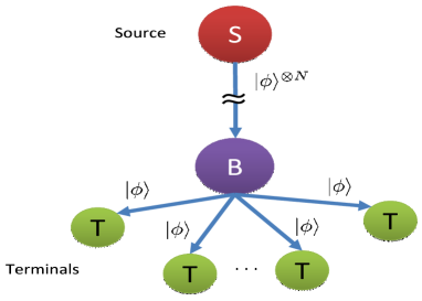
Figure 1: (Color online) Quantum multicast networks that contain a single source (labeled as $S$) and $N$ terminals (labeled as $T$). The source $S$ can generate $N$ copies of an identical quantum state $|\phi\rangle$. The multicasting task is for the source $S$ to distribute the quantum state $|\phi\rangle$ to each terminal $T$ simultaneously and perfectly through the link that connects the source $S$ and the node $B$.

We propose a recursive encoding circuit that can provide a trade-off between the hardware complexity and the bandwidth consumption. The idea is, instead of encoding $N$ copies of the quantum state $|\phi\rangle$ as a whole, to divide the quantum data $|\phi\rangle^{\otimes N}$ into $\frac{N}{k}$ groups where each group contains $k$ copies of the state $|\phi\rangle$. We then encode each of these groups to a quantum state, say $|\phi^{\prime}\rangle$, by a smaller encoding unitary $U^{k}_{d}$ of size $d^{k}\times d^{k}$. The dimension of the compressed state $|\phi^{\prime}\rangle$ is $\mathrm{\textbf{H}}^{k}_{d}$. Finally, we encode $\frac{N}{k}$ copies of the state $|\phi^{\prime}\rangle$ by another encoding unitary matrix $U^{N/k}_{\mathrm{\textbf{H}}^{k}_{d}}$. The above 2-step encoding process can be generalized to the following recursive encoding:

1. If $N=1$, abort. Otherwise, divide $N$ copies of the quantum state $|\phi\rangle$ into smaller groups, where each group contains $k$ copies of the state $|\phi\rangle$. Denote $|\Phi\rangle\equiv|\phi\rangle^{\otimes k}$.

2. Encode the quantum state $|\Phi\rangle$ in each group by the encoding unitary $U^{k}_{d}$ .

3. Throw away the first $(k-\log_{d}\mathrm{\textbf{H}}^{k}_{d})$ redundant qudits. Denote by $|\Phi^{\prime}\rangle$ the rest $(\log_{d}\mathrm{\textbf{H}}^{k}_{d})$-qudit quantum state.

4. Set $N\leftarrow\frac{N}{k}$, $d\leftarrow\mathrm{\textbf{H}}^{k}_{d}$, and $|\phi\rangle\leftarrow|\Phi^{\prime}\rangle$. Go to step 1.

We refer to this process as the recursive homogeneous encoding.

Denote by $y_{n}$ the dimension of the compressed quantum state $|\Phi^{\prime}\rangle$ at $n^{th}$ step of the above recursive procedure. Let $y_{0}=d$, which corresponds to the dimension of the original quantum state $|\phi\rangle$. We then have the following recursive relation:

$$y_{n+1}=\mathrm{\textbf{H}}^{k}_{y_{n}}.$$ (8)

Let $L_{n}$ denote the number of the remaining qudits after the $n^{th}$ recursion:

$$L_{n}=\log_{d}y_{n}.$$ (9)

In our recursive protocol, there are $n^{*}\equiv\log_{k}N$ recursions. Denote by $L=L_{n^{*}}$ the number of remaining qudits after the last encoding unitary. The parameter $L$ describes the minimal bandwidth requirement for the link connecting the source $S$ and the node $B$ in Fig. 1 when the source $S$ employs our recursive homogeneous encoding.

Denote by $D$ the dimension of the input quantum states to the last encoding unitary:

$$D=y^{k}_{n^{*}-1}.$$ (10)

The parameter $D$ captures the complexity of the recursive encoding circuit. Obviously, the values of $L$ and $D$ depend on the controlling parameter $k$, which corresponds to the size of each group in our recursive procedure. By varying $k$ in our recursive procedure, we can provide a trade-off between the bandwidth requirement $L$ and the encoding complexity $D$. An example of the recursive homogeneous encoding circuit with $d=2,k=4,N=64$ is illustrated in Fig. 2.

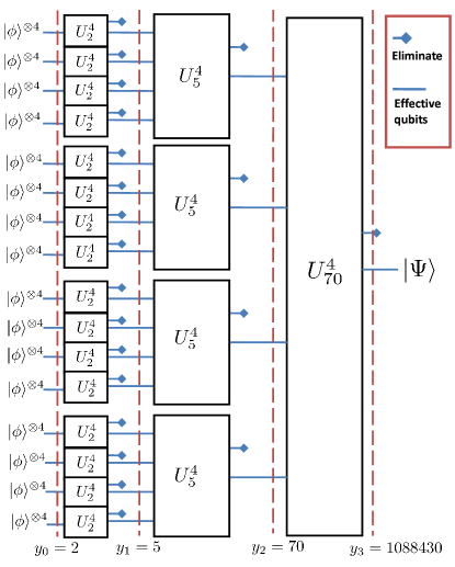
Figure 2: An example of the recursive homogeneous encoding circuit for the single-source, $N$-terminal multicast quantum networks. The source generates $N$ copies of the quantum state $|\phi\rangle$ in ${\cal H}_{d}$, and runs the recursive homogeneous encoding circuit to output the encoded quantum state $|\Psi\rangle$. Let $d=2,k=4,N=64$. There are $\log_{k}N=3$ recursions in the example. In the $n^{th}$ recursion, the encoding unitary $U_{y_{n-1}}^{k}$, where $y_{n}$ represents the dimension of the encoded quantum state after $U_{y_{n-1}}^{k}$, is applied to encode each group of group size $k$. The dimension of the input quantum system to the last encoding unitary (the encoding complexity) is $D=70^{4}\approx 2.4\times 10^{6}$, compared to the encoding complexity, $2^{64}\approx 1.84\times 10^{19}$, without recursive homogeneous encoding.

In the following, we will derive a relation between the minimal bandwidth requirement $L$ and the size $k$ of each group, and a relation between the encoding complexity $D$ and the size $k$ of each group in our recursive procedure. First, following (8), we have $k\ll y_{n}$ when $n\geq 2$. Then we can approximate the term $y_{n+1}=\mathrm{\textbf{H}}^{k}_{y_{n}}$ by:

$$y_{n+1}=\mathrm{\textbf{H}}^{k}_{y_{n}}\simeq\frac{{y^{k}_{n}}}{k!}=\frac{{y^{k}_{n}}}{d^{c}},$$ (11)

where we choose a constant $c$ such that $d^{c}=k!$. Followed from (9), we have

$$L_{n} =\log_{d}y_{n}$$

$$=\log_{d}\left(\frac{{y^{k}_{n-1}}}{d^{c}}\right)$$

$$=k\log_{d}(y_{n-1})-c$$

$$=kL_{n-1}-c.$$ (12)

The second equality uses (8) and (11), and the last equality uses (9). Solving the linear recursive equation (12) gives

$$L_{n}=k^{n-2}L_{2}-\frac{k^{n-2}-1}{k-1}c,$$ (13)

where $L_{2}$ can be derived from (8):

$$L_{2}=\log_{d}\frac{(2k)!}{k!k!}.$$

Substituting $N$ for $k^{n^{*}}$ in (13), we obtain the first desired relation between $L=L_{n^{*}}$ and $k$:

$$L=\frac{N}{k^{2}}L_{2}-\left(\frac{N}{k^{2}}-1\right)\frac{c}{k-1}.$$ (14)

We can obtain the other desired relation between $D$ and $k$ as follows:

$$\log_{d}D =k\log_{d}y_{n^{*}-1}$$

$$=kL_{n^{*}-1}$$

$$=L+c$$

$$=\frac{N}{k^{2}}(L_{2}-\frac{c}{k-1})+\frac{ck}{k-1}.$$

The first equality uses (10). The second equality uses (9). The third equality uses (12). The final equality uses (14).

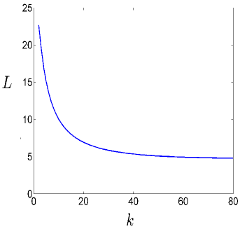
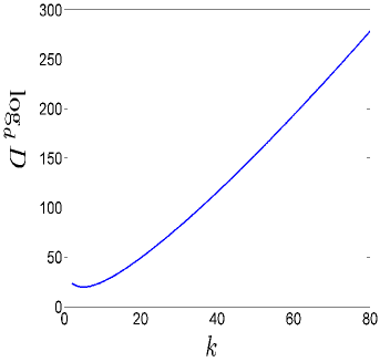
(a)	(b)

Figure 3: (Color online) Figure (a) depicts the numerical evaluation of the trade-off between the minimal bandwidth requirement $L$ (the number of qudits per channel use) and the group size $k$ in each recursive procedure. Figure (b) depicts the numerical evaluation of the trade-off between the encoding complexity $D$ and the group size $k$ in each recursive procedure. We show $\log_{d}D$ in this figure, which corresponds to the number of input qudits to the final encoding unitary. In both figures, we set $N=80$ and $d=2$. When the controlling parameter $k$ is small, the bandwidth requirement $L$ is large, but the encoding complexity is low. When $k$ is large, the bandwidth requirement $L$ is small, but the encoding complexity $D$ is high.

We plot $L$ versus $k$ in Fig. 3(a), and plot $\log_{d}D$ versus $k$ in Fig. 3(b). From Fig. 3, we can see that the group size $k$ in the recursive procedure provides a trade-off between minimal bandwidth requirement $L$ and the encoding complexity $D$. When $k$ is small, the bandwidth requirement $L$ is large, but the encoding complexity is low. When $k$ is large, the bandwidth requirement $L$ is small, but the encoding complexity $D$ is high. Notice that when $k=N$, we recover Shi and Soljanin’s result in [10].

4 Heterogeneous encoding in quantum multicast networks

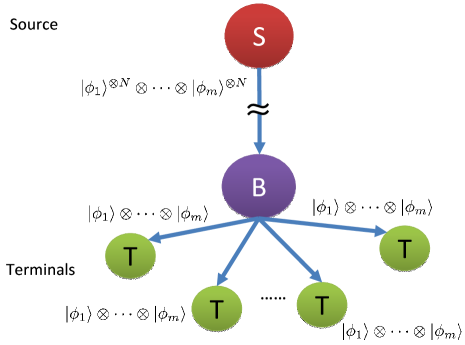
Figure 4: (Color online) Quantum multicast networks that contain a single source (labeled as $S$) and $N$ terminals (labeled as $T$). The source $S$ can generate $N$ copies of the heterogeneous quantum state $|\Phi\rangle\equiv|\phi_{1}\rangle\otimes\cdots\otimes|\phi_{m}\rangle$. The multicasting task is for $S$ to distribute the quantum state $|\Phi\rangle$ to each terminal $T$ simultaneously and perfectly through the link that connects the source $S$ and the node $B$.

The main result of this section is the development of two lossless compressing schemes for the quantum multicast network depicted in Fig. 4. The network contains a single source and $N$ terminals. The source $S$ can generate $N$ copies of the quantum state $|\Phi\rangle\equiv|\phi_{1}\rangle\otimes\cdots\otimes|\phi_{m}\rangle$ in ${\cal H}_{d}^{\otimes m}$. The multicasting task is for the source $S$ to distribute the quantum state $|\Phi\rangle$ to each terminal $T$ simultaneously and perfectly through the link that connects the source $S$ and the node $B$. If no encoding is performed at the source $S$, the bandwidth (edge capacity) between the source $S$ and the node $B$ must be as large as $Nm$ qudits for the source to transmit $|\Phi\rangle^{\otimes N}$ faithfully. We can also apply Shi and Soljanin’s homogeneous encoding [10], or the recursive homogeneous encoding introduced in the previous section, to encode each $|\phi_{i}\rangle^{\otimes N}$, $i=1,2,\cdots,m$.

However, there is a possibility that we can design better lossless compression schemes than the homogeneous encoding if we know the structure of the set of quantum states $\{|\phi_{1}\rangle,\cdots,|\phi_{m}\rangle\}$ generated by the source $S$. One such example is when the coefficients of the quantum state $|\phi_{i}\rangle$ in the set $\{|\phi_{1}\rangle,\cdots,|\phi_{m}\rangle\}$ are equal to the permutation of the coefficients of another quantum state $|\phi_{j}\rangle$ in the set. We formally define the set of quantum states whose coefficients are the same after permutation as follows.

Definition 1

Given is the set of coefficients $\boldsymbol{\alpha}\equiv\{\alpha_{0},\alpha_{1},\cdots,\alpha_{d-1}\}$, where $\sum_{i=0}^{d-1}|\alpha_{i}|^{2}=1$ and let $|x_{0}\rangle\equiv\sum_{i=0}^{d-1}\alpha_{i}|i\rangle$. We denote by $X(\boldsymbol{\alpha})$ the collection of all the quantum states whose coefficients are the same after all possible permutations:

$$X(\boldsymbol{\alpha})\equiv\left\{|\phi\rangle:\forall P,\ |\phi\rangle=P|x_{0}\rangle\right\},$$

where $P$ is an arbitrary $d\times d$ permutation matrix. For example, $X(\{\alpha,\beta\})=\{\alpha|0\rangle+\beta|1\rangle,\beta|0\rangle+\alpha|1\rangle\}$, where $|\alpha|^{2}+|\beta|^{2}=1$.

We propose two lossless compression schemes with improvement power for compressing heterogeneous quantum data $\{|\phi_{1}\rangle,\cdots,|\phi_{m}\rangle\}$, if the quantum data generated by the source $S$ is a subset of $X(\boldsymbol{\alpha})$ for a given $\boldsymbol{\alpha}$.

Before introducing these two lossless compression schemes, we first show that there exists a heterogeneous encoding for compressing the set of quantum states $\{|\phi_{1}\rangle,\cdots,|\phi_{m}\rangle\}\subset X(\boldsymbol{\alpha})$. Let $|\Phi\rangle\equiv|\phi_{1}\rangle\otimes\cdots\otimes|\phi_{m}\rangle$. It is not difficult to see that there are $\mathrm{\textbf{H}}^{m}_{d}=C^{m+d-1}_{d}$ different coefficients $\{\gamma_{t}\}$ in the state $|\Phi\rangle$, and we can represent the state $|\Phi\rangle$ as follows:

$$|\Phi\rangle=\sum_{t=0}^{\mathrm{\textbf{H}}^{m}_{d}-1}\gamma_{t}|\boldsymbol{e}_{t}\rangle,$$ (15)

where $|\boldsymbol{e}_{t}\rangle$ is similarly defined in (3) and the set $\{|\boldsymbol{e}_{t}\rangle\}$ forms a permutation-invariant basis for ${\cal H}_{d}^{\otimes m}$. Then there exists a unitary $S$ such that

$$S|\boldsymbol{e}_{t}\rangle=|0\rangle^{\otimes(m-\log_{d}\mathrm{\textbf{H}}^{m}_{d})}\otimes|t\rangle,$$ (16)

where $\{|t\rangle\}$ forms an orthonormal basis for ${\cal H}_{d}^{\otimes\log_{d}\mathrm{\textbf{H}}^{m}_{d}}$. Applying this unitary $S$ to the heterogeneous quantum state $|\Phi\rangle$ gives

$$S|\Phi\rangle=|0\rangle^{\otimes(m-\log_{d}\mathrm{\textbf{H}}^{m}_{d})}\otimes\left(\sum_{t=0}^{\mathrm{\textbf{H}}^{m}_{d}-1}\gamma_{t}|t\rangle\right).$$ (17)

Denote $|\Phi^{\prime}\rangle=\sum_{t=0}^{\mathrm{\textbf{H}}^{m}_{d}-1}\gamma_{t}|t\rangle$. The unitary $S$ in (16) implements a lossless compression that compresses the heterogeneous quantum state $|\Phi\rangle$ of dimension $d^{m}$ to the state $|\Phi^{\prime}\rangle$ of dimension $\mathrm{\textbf{H}}_{d}^{m}$:

$$RS|\Phi\rangle=\sum_{t=0}^{\mathrm{\textbf{H}}^{m}_{d}-1}\gamma_{t}|t\rangle=|\Phi^{\prime}\rangle,$$ (18)

where $R$ is the operation that removes the ancilla state $|0\rangle^{\otimes(m-\log_{d}\mathrm{\textbf{H}}^{m}_{d})}$ in (17). Furthermore, the compression is lossless because we can recover the original state $|\Phi\rangle$ from $|\Phi^{\prime}\rangle$ as follows:

$$S^{-1}A|\Phi^{\prime}\rangle=|\Phi\rangle,$$ (19)

where $A$ is the operation that adds the ancilla state $|0\rangle^{\otimes(m-\log_{d}\mathrm{\textbf{H}}^{m}_{d})}$ to $|\Phi^{\prime}\rangle$.

In the following, we will propose two new encoding structures that are better (in terms of bandwidth requirement) than simply encoding each state $|\phi_{i}\rangle^{\otimes N}$ separately with the homogeneous encoding when the set of quantum states $\{|\phi_{1}\rangle,\cdots,|\phi_{m}\rangle\}$ generated by the source is a subset of $X(\boldsymbol{\alpha})$ for a given coefficient set $\boldsymbol{\alpha}$.

4.1 Homo-hetero encoding

The first method for multicasting $\{|\phi_{1}\rangle,\cdots,|\phi_{m}\rangle\}\subset X(\boldsymbol{\alpha})$ is to first use the homogeneous encoding reviewed in $(\ref{singleencode1})$ separately on each $|\Phi_{i}\rangle\equiv|\phi_{i}\rangle^{\otimes N}$ to output an encoded state $|\Phi_{i}^{\prime}\rangle$, $\forall i$. It is not difficult to see that the number of different coefficients in each $|\Phi_{i}\rangle$ is equal to $\mathrm{\textbf{H}}^{N}_{d}$. Denote by $\boldsymbol{\beta}_{i}$ the collection of all possible coefficients in $|\Phi_{i}\rangle$. Each set $\boldsymbol{\beta}_{i}$ is the same because $\{|\phi_{1}\rangle,\cdots,|\phi_{m}\rangle\}\subset X(\boldsymbol{\alpha})$. Therefore we can remove the subscript and denote by $\boldsymbol{\beta}$. The set of quantum states $\{|\Phi_{1}^{\prime}\rangle,\cdots,|\Phi_{m}^{\prime}\rangle\}$ is a subset of $X(\boldsymbol{\beta})$, since each state $|\Phi_{i}^{\prime}\rangle$ shares the same set of coefficients as the state $|\Phi_{i}\rangle$. This allows us to encode $|\Phi_{1}^{\prime}\rangle\otimes\cdots\otimes|\Phi_{m}^{\prime}\rangle$ by the heterogeneous encoding introduced in (16) to an encoded output state $|\Omega\rangle$ of dimension $\mathrm{\textbf{H}}^{m}_{\mathrm{\textbf{H}}^{N}_{d}}$. We illustrate the above home-hetero encoding in Fig. 5.

The encoding process can be represented by the following expression:

$$|\Omega\rangle=RS\left((RU|\Phi_{1}\rangle)\otimes\cdots\otimes(RU|\Phi_{m}\rangle)\right),$$ (20)

where $|\Phi_{i}\rangle\equiv|\phi_{i}\rangle^{\otimes N}$, $U$ and $S$ are the homogeneous encoding (4) and the heterogeneous encoding (16), respectively, and $R$ is the operation that removes the redundant ancilla states.

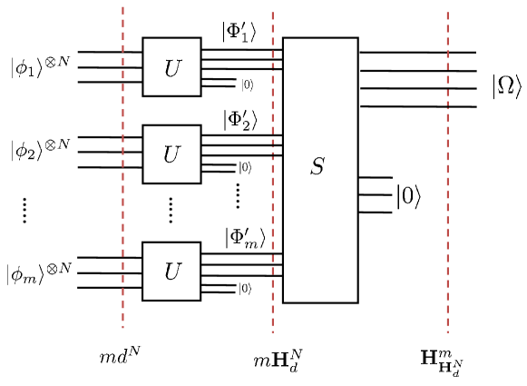
Figure 5: (Color online) Quantum circuit for the homo-hetero encoding. The homo-hetero encoding first uses the homogeneous encoding unitary $U$ to encode each $|\phi_{i}\rangle^{\otimes N}$ of dimension $d^{N}$ into an encoded state $|\Phi_{i}^{\prime}\rangle$. The dimension of each encoded state $|\Phi_{i}^{\prime}\rangle$ is $\mathrm{\textbf{H}}^{N}_{d}$. Then the heterogeneous encoding unitary $S$ is applied to encode $|\Phi_{1}^{\prime}\rangle\otimes\cdots\otimes|\Phi_{m}^{\prime}\rangle$ into the final state $|\Omega\rangle$ of dimension $\mathrm{\textbf{H}}^{m}_{\mathrm{\textbf{H}}^{N}_{d}}$. The circuit implements a lossless compression that compresses the state $|\phi_{1}\rangle^{\otimes N}\otimes\cdots\otimes|\phi_{m}\rangle^{\otimes N}$ of dimension $md^{N}$ to the encoded state $|\Omega\rangle$ of dimension $\mathrm{\textbf{H}}^{m}_{\mathrm{\textbf{H}}^{N}_{d}}$.

The homo-hetero encoding implements a lossless compression that compresses the state $|\Phi_{1}\rangle\otimes\cdots\otimes|\Phi_{m}\rangle$ of dimension $md^{N}$ to the encoded state $|\Omega\rangle$ of dimension $\mathrm{\textbf{H}}^{m}_{\mathrm{\textbf{H}}^{N}_{d}}$. This homo-hetero encoding is lossless because we can recover the original state $|\Phi_{1}\rangle\otimes\cdots\otimes|\Phi_{m}\rangle$ as follows :

$$|\Phi_{1}^{\prime}\rangle\otimes\cdots\otimes|\Phi_{m}^{\prime}\rangle =S^{-1}A|\Omega\rangle$$

$$|\Phi_{1}\rangle\otimes\cdots\otimes|\Phi_{m}\rangle =(U^{-1}A|\Phi_{1}^{\prime}\rangle)\otimes\cdots\otimes(U^{-1}A|\Phi_{m}^{\prime}\rangle),$$

where $A$ is the operator that adds the necessary ancilla states. The node $B$ in Fig. 4 first adds enough amount of the ancilla states to the state $|\Omega\rangle$. Next he can recover the states $|\Phi_{1}^{\prime}\rangle\otimes\cdots\otimes|\Phi_{m}^{\prime}\rangle$ by performing the inverse heterogeneous encoding $S^{-1}$. Then he adds enough number of the ancilla states to each state $|\Phi_{i}^{\prime}\rangle$, and performs the inverse homogeneous encoding $U^{-1}$ to generate $N$ copies of the original data $|\phi_{i}\rangle$, $\forall i$. Finally he distributes the quantum states to the terminals.

4.2 Hetero-homo encoding

The second method for multicasting $\{|\phi_{1}\rangle,\cdots,|\phi_{m}\rangle\}\subset X(\boldsymbol{\alpha})$ is to first apply the heterogeneous encoding $S$ (16) to the state $|\Phi\rangle\equiv|\phi_{1}\rangle\otimes\cdots\otimes|\phi_{m}\rangle$, and outputs the encoded state $|\Phi^{\prime}\rangle$ of dimension $\mathrm{\textbf{H}}^{m}_{d}$. Next, the homogeneous encoding $U$ (4) is applied to encode $|\Phi^{\prime}\rangle^{\otimes N}$ of dimension $(\mathrm{\textbf{H}}^{m}_{d})^{N}$ to an encoded state $|\Omega\rangle$ of dimension $\mathrm{\textbf{H}}^{N}_{\mathrm{\textbf{H}}^{m}_{d}}$. We illustrate the above home-hetero encoding in Fig. 6.

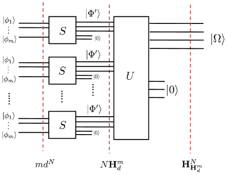
Figure 6: (Color online) Quantum circuit for the hetero-homo encoding. The hetero-homo encoding first uses the heterogeneous encoding unitary $S$ to encode each $|\Phi\rangle\equiv|\phi_{1}\rangle\otimes\cdots\otimes|\phi_{m}\rangle$ into an encoded state $|\Phi^{\prime}\rangle$. The dimension of the encoded state $|\Phi^{\prime}\rangle$ is $\mathrm{\textbf{H}}^{m}_{d}$. Then the homogeneous encoding unitary $U$ is applied to encode $|\Phi^{\prime}\rangle^{\otimes N}$ into the final state $|\Omega\rangle$ of dimension $\mathrm{\textbf{H}}^{N}_{\mathrm{\textbf{H}}^{m}_{d}}$. The circuit implements a lossless compression that compresses the state $|\phi_{1}\rangle^{\otimes N}\otimes\cdots\otimes|\phi_{m}\rangle^{\otimes N}$ of dimension $md^{N}$ to the encoded state $|\Omega\rangle$ of dimension $\mathrm{\textbf{H}}^{N}_{\mathrm{\textbf{H}}^{m}_{d}}$.

The hetero-homo encoding process can be expressed as:

$$|\Omega\rangle=RU\left(RS(|\phi_{i}\rangle\otimes\cdots\otimes|\phi_{m}\rangle)\right)^{\otimes N},$$ (21)

where $U$ and $S$ are the homogeneous encoding (4) and the heterogeneous encoding (16), respectively, and $R$ is the operation that removes the redundant ancilla states.

The hetero-homo encoding implements a lossless compression that compresses the state $|\Phi\rangle^{\otimes N}$ of dimension $md^{N}$ to the encoded state $|\Omega\rangle$ of dimension $\mathrm{\textbf{H}}^{N}_{\mathrm{\textbf{H}}^{m}_{d}}$. This hetero-homo encoding is lossless because we can recover the original state $|\Phi\rangle^{\otimes N}$ as follows:

$$|\Phi^{\prime}\rangle^{\otimes N} =U^{-1}A|\Omega\rangle$$

$$|\Phi\rangle^{\otimes N} =(S^{-1}A|\Phi^{\prime}\rangle)^{\otimes N},$$

where $A$ is the operation that adds the necessary ancilla states. The node $B$ in Fig. 4 first adds enough amount of the ancilla states to the state $|\Omega\rangle$. Next he can recover the states $|\Phi^{\prime}\rangle$ by performing the inverse homogeneous encoding $U^{-1}$. Then he adds enough number of the ancilla states to the state $|\Phi^{\prime}\rangle$, and performs the inverse heterogeneous encoding $S^{-1}$ to generate $N$ copies of the original data $|\Phi\rangle$. Finally he distributes the quantum states to the terminals.

4.3 Comparison and analysis

Table 1 lists the minimal bandwidth requirement of different encoding methods employed by the source in quantum multicast networks in Fig. 4. The quantum multicast networks contain a single source and $N$ terminals. The set of quantum states $\{|\phi_{1}\rangle,\cdots,|\phi_{m}\rangle\}$, $\forall i$ $|\phi_{i}\rangle$ in ${\cal H}_{d}$, to be multicast to each terminal is heterogeneous and is a subset of $X(\boldsymbol{\alpha})$ for a given $\boldsymbol{\alpha}$. The source can perform either one of the following four encoding techniques: multicasting simultaneously without encoding, the homogeneous encoding (4), the homo-hetero encoding introduced in section 4.1, and the hetero-homo encoding introduced in section 4.2.

Types of Multicasting	Bandwidth Requirement
Multicasting directly	$Nm$
Homogeneous encoding	$m\log_{d}\mathrm{\textbf{H}}^{N}_{d}$
Homo-hetero encoding	$\log_{d}\mathrm{\textbf{H}}^{m}_{\mathrm{\textbf{H}}^{N}_{d}}$
Hetero-homo encoding	$\log_{d}\mathrm{\textbf{H}}^{N}_{\mathrm{\textbf{H}}^{m}_{d}}$

Table 1: Comparison of minimal bandwidth requirements between the source $S$ and the node $B$ in quantum multicast networks in Fig. 4. The set of quantum states to be multicast to each terminal is of size $m$, and is a subset of $X(\boldsymbol{\alpha})$ for a given set of coefficients $\boldsymbol{\alpha}=\{\alpha_{i}\}_{i=0}^{d-1}$. The source can perform either one of the following four encoding techniques: multicasting simultaneously without encoding, the homogeneous encoding (4), the homo-hetero encoding introduced in section 4.1, and the hetero-homo encoding introduced in section 4.2.

We numerically evaluate the minimal bandwidth requirements of the three non-trivial encoding schemes in Fig. 7. We investigate how the size $m$ of the set of heterogeneous quantum states and the number $N$ of terminals affect the minimal bandwidth requirements of different encoding schemes. We have the following observations. First, our homo-hetero encoding is always better than the homogeneous encoding because we perform an extra heterogeneous encoding (16) to take advantage of the structure of the encoded quantum states of the homogeneous encoding. Second, the heterogeneous encoding schemes show obvious gain over the homogeneous encoding when the size $m$ of the set of heterogeneous quantum states is large (see Fig. 7(b)). This is because the compressing power of the heterogeneous encoding becomes evident when there exists abundant redundancy in the heterogeneous quantum states. Fig. 7(b) shows that the hetero-homo encoding outperforms the other two encodings when $N$ is smaller than $m$, while the homo-hetero encoding takes the lead when $N$ is larger than $m$. The reason is the following. When $N$ is large, the redundancy arises mainly from each quantum state $|\phi_{i}\rangle^{\otimes N}$, $\forall i$. Therefore, the first homogeneous compression of the homo-hetero encoding can remove more redundancy than the first heterogeneous compression of the hetero-homo encoding. On the other hand, when $N$ is small, the redundancy mainly comes from the set of heterogeneous quantum states. Hence, the first heterogeneous compression of the hetero-homo encoding can remove the redundancy more efficiently than the first homogeneous compression of the homo-hetero encoding. It also justifies that the cross point of the minimal bandwidth requirements of these two heterogeneous encodings occurs when $m=N$.

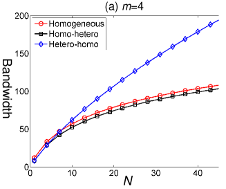
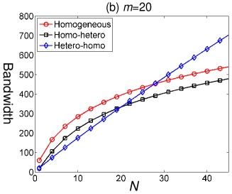
Figure 7: (Color online) Numerical evaluation of the minimal bandwidth requirements of the three non-trivial encoding schemes: the homogeneous encoding (4), the homo-hetero encoding introduced in section 4.1, and the hetero-homo encoding introduced in section 4.2. The vertical axis represents the minimal bandwidth requirement (the number of qudits per channel use, $d=8$). The horizontal axis represents the number $N$ of terminals in quantum multicast networks. We investigate how the size $m$ of the set of heterogeneous quantum states and the number $N$ of terminals affect the minimal bandwidth requirements of different encoding schemes. Figure (a) corresponds to $m=3$, and Figure (b) corresponds to $m=20$.

5 Other quantum multicast networks

In this section, we will consider the quantum multicast networks other than the single-source, $N$-terminal model depicted in Fig. 4. Two examples are discussed. One is the $m$-source, $N$-terminal quantum multicast networks, and the other is the quantum multicast networks with ring topology. We then analyze the bandwidth requirements of these two quantum multicast networks, where different encoding schemes are employed.

5.1 Multi-source Multi-terminal networks

One generalization of the single-source, $N$-terminal multicast model is the $m$-source, $N$-terminal multicast model depicted in Fig. 8. The $i^{th}$ source $S$ can generate $N$ copies of a quantum state $|\phi_{i}\rangle$ in ${\cal H}_{d}$, $i=1,2,\cdots,m$, such that the set of quantum states $\{|\phi_{1}\rangle,\cdots,|\phi_{m}\rangle\}$ is a subset of $X(\boldsymbol{\alpha})$ for a given $\boldsymbol{\alpha}$. The multicasting task is for each of the sources to distribute his own quantum state, say $|\phi_{i}\rangle$, $i=1,2,\cdots,m$, to each terminal simultaneously and perfectly through the link that connects the node $X$ and the node $B$. If no encoding is performed at the node $X$, the bandwidth required between the node $X$ and the node $B$ must be as large as $Nm$ qudits per channel use. The node $X$ can also perform either the homogeneous or the heterogeneous encoding to compress the quantum states. The minimal bandwidth requirements of the link connecting the node $X$ and the node $B$ are depicted in Table 1, depending on the encoding technique employed by the node $X$.

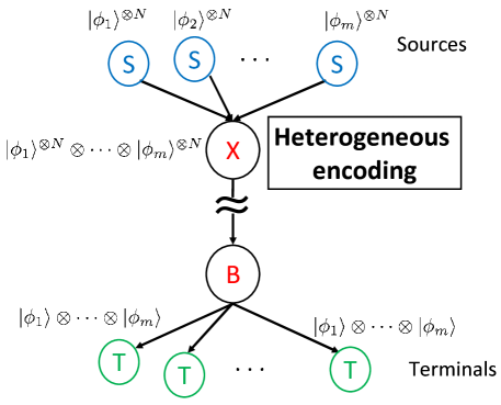
Figure 8: (Color online) Quantum multicast networks that contain $m$ sources (labeled as $S$) and $N$ terminals (labeled as $T$). The $i^{th}$ source $S$ can generate $N$ copies of a quantum state $|\phi_{i}\rangle$, $i=1,2,\cdots,m$. The multicasting task is for each of the sources to distribute his own quantum state, say $|\phi_{i}\rangle$, to each terminal $T$ simultaneously and perfectly through the link that connects the node $X$ and the node $B$. If the set of quantum states $\{|\phi_{1}\rangle,\cdots,|\phi_{m}\rangle\}$ generated by the sources is a subset of $X(\boldsymbol{\alpha})$ for a given $\boldsymbol{\alpha}$, the heterogeneous encoding can be applied at the node $X$ to efficiently compress the quantum states.

5.2 Ring networks

We consider the quantum ring networks depicted in Fig. 9. The networks contain a single-source $S$ and $N$ number of nodes on a ring. Each node $B$ connects to $m$ number of terminals, and forms a cluster. We consider the following multitasking task with the assumption that $N\gg m$: the source $S$ would like to simultaneously and perfectly distribute the $i^{th}$ quantum state in $\{|\phi_{1}\rangle,\cdots,|\phi_{m}\rangle\}$ to the $i^{th}$ terminal in each of the $N$ clusters, $\forall i$. The source $S$ can use the clockwise and counterclockwise paths to distribute the quantum states to destinations. We will evaluate the overall bandwidth required on the ring in order for $S$ to accomplish the desired multicasting task.

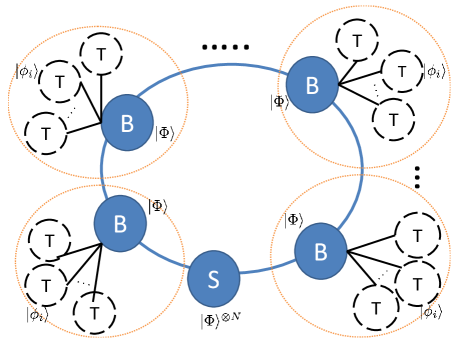
Figure 9: (Color online) The quantum multicast networks with ring topology that contain a single-source (labeled by $S$), and $N$ nodes (labeled by $B$) on a ring. Each node $B$ connects to $m$ terminals (labeled by $T$), and forms a cluster. The source $S$ can generate $N$ copies of the quantum state $|\Phi\rangle\equiv|\phi_{1}\rangle\otimes\cdots\otimes|\phi_{m}\rangle$. The multitasking task is for the source $S$ to perfectly distribute the $i^{th}$ quantum state in $\{|\phi_{1}\rangle,\cdots,|\phi_{m}\rangle\}$ to the $i^{th}$ terminal in each of the $N$ clusters, $\forall i$.

If no encoding is applied, the source simply sends $\frac{N}{2}$ copies of the quantum state $|\Phi\rangle$, where $|\Phi\rangle\equiv|\phi_{1}\rangle\otimes\cdots\otimes|\phi_{m}\rangle$, down to both the clockwise and counterclockwise paths. The first node on both sides distributes one copy of the state $|\Phi\rangle$ to the $m$ terminals in his cluster, and forwards the rest $\frac{N}{2}-1$ copies of the state $|\Phi\rangle$ to the next node. The process continues until all the terminals receive a desired quantum state. We can then evaluate the overall bandwidth required on the ring as follows:

$$2m\sum^{\frac{N}{2}}_{k=1}k=m\frac{N}{2}(\frac{N}{2}+1).$$ (22)

The bandwidth consumption without encoding is $O(N^{2})$.

If the source and the $N$ number of nodes on the ring employ the homogeneous encoding, the multicasting task proceeds as follows. For each $i=1,2,\cdots,m$, the source $S$ applies two instances of the homogeneous encoding on $\frac{N}{2}$ copies of the state $|\phi_{i}\rangle$, and then sends the encoded states down to both paths. The dimension of the encoded quantum state on either path is $m\mathrm{\textbf{H}}^{\frac{N}{2}}_{d}$. After receiving the encoded quantum state, the first node on both sides performs the inverse of the homogeneous encoding to recover the original state $|\Phi\rangle^{\otimes\frac{N}{2}}$, distributes one copy of the state $|\Phi\rangle$ to the terminals in his cluster, and then applies the homogeneous encoding again to encode the rest $\frac{N}{2}-1$ copies of the state $|\Phi\rangle$. The dimension of the encoded state now becomes $m\mathrm{\textbf{H}}^{\frac{N}{2}-1}_{d}$. The process continues until all the terminals receive a desired quantum state. We can then evaluate the overall bandwidth required on the ring when each node applies the homogeneous encoding as follows:

$$2m\sum^{\frac{N}{2}}_{k=1}\log_{d}\mathrm{\textbf{H}}^{k}_{d} = 2m\sum_{k=1}^{\frac{N}{2}}\log_{d}\frac{(k+d-1)!}{d!(k-1)!}$$ (23)

$$= 2m\sum_{\ell=0}^{d-1}\sum_{k=1}^{\frac{N}{2}}\log_{d}(k+\ell)-mN\log_{d}d!$$

$$\simeq 2md\sum^{\frac{N}{2}}_{k=1}\log_{d}k-mN\log_{d}d!$$

$$\simeq mNd\log_{d}\frac{N}{2}.$$ (24)

The first approximation follows from the assumption $N\gg d$. The second approximation holds because $mN\log_{d}d!$ is much smaller the first term in (23) and it can be evaluated by the following:

$$\sum^{N/2}_{k=1}\log_{d}k\simeq\int^{N/2}_{1}\log_{d}kdk=\frac{1}{\ln d}\left(k\ln k-k\right)\mid^{\frac{N}{2}}_{1}.$$

If the source and the $N$ number of nodes on the ring employ the heterogeneous encoding, the multicasting task proceeds as follows. Specifically, we will use the homo-hetero encoding because it outperforms the hetero-homo encoding when $N\gg m$. The source $S$ applies two instances of the homo-hetero encoding on $\frac{N}{2}$ copies of the state $|\Phi\rangle$, and then sends the two encoded states down to both paths. The dimension of the encoded quantum state in either path is $\mathrm{\textbf{H}}^{m}_{\mathrm{\textbf{H}}^{\frac{N}{2}}_{d}}$. After receiving the encoded quantum state, the first node on both sides performs the inverse of the homo-hetero encoding to recover the original state $|\Phi\rangle^{\otimes\frac{N}{2}}$, distributes one copy of the state $|\Phi\rangle$ to the terminals in his cluster, and then applies the homo-hetero encoding again to encode the rest $\frac{N}{2}-1$ copies of the state $|\Phi\rangle$. The dimension of the encoded state now becomes $\mathrm{\textbf{H}}^{m}_{\mathrm{\textbf{H}}^{\frac{N}{2}-1}_{d}}$. The process continues until all the terminals receive a desired quantum state. We can then evaluate the overall bandwidth required on the ring when each node applies the homo-hetero encoding as follows:

$$2\sum_{k=1}^{\frac{N}{2}}\log_{d}\mathrm{\textbf{H}}^{m}_{\mathrm{\textbf{H}}^{k}_{d}} = 2\sum_{k=1}^{\frac{N}{2}}\log_{d}\frac{\left(m+\mathrm{\textbf{H}}^{k}_{d}-1\right)!}{(m-1)!\mathrm{\textbf{H}}^{k}_{d}!}$$ (25)

$$= 2\sum_{\ell=1}^{m-1}\sum_{k=1}^{\frac{N}{2}}\log_{d}\left(\mathrm{\textbf{H}}^{k}_{d}+\ell\right)-N\log_{d}(m-1)!$$

$$\simeq 2(m-1)\sum_{k=1}^{\frac{N}{2}}\log_{d}\mathrm{\textbf{H}}^{k}_{d}-N\log_{d}(m-1)!$$

$$\simeq (m-1)Nd\log_{d}\frac{N}{2}.$$ (26)

The first approximation holds because $\mathrm{\textbf{H}}^{k}_{d}$ is usually very large. The second approximation follows from (24):

$$\sum_{k=1}^{\frac{N}{2}}\log_{d}\mathrm{\textbf{H}}^{k}_{d}\simeq\frac{N}{2}d\log_{d}\frac{N}{2}.$$

The overall bandwidth consumed by both the homogeneous and heterogeneous encoding is $O(N\log N)$. The bandwidth saved due to encoding is on the order of $O(\frac{1}{N}\log N)$.

6 Conclusion

The achievement of this paper is two-fold. First, we proposed a novel recursive homogeneous encoding to realize quantum multicasting with low encoder complexity in section 3. Our recursive homogeneous encoding circuit can provide a reasonable trade-off between the encoder complexity and the dimension of the encoded state (corresponds to the bandwidth requirement of the quantum networks). Though the encoding proposed by Shi and Soljanin [10] reduced the minimal bandwidth requirement from $N$ to $\log_{d}\mathrm{\textbf{H}}^{N}_{d}$, the hardware complexity of their encoding circuit is daunting. Hence, it is difficult to practically implement their encoder in quantum multicast networks. Our recursive encoding idea proves to be extremely useful in the situation where the technology of producing large-scale quantum circuits is limited. We detailed the relation between the minimal bandwidth requirement and the encoding complexity. One can easily decide the dimension of the compressed state and the encoder complexity by our formula. We also analyzed how the relation is affected by the size $k$ of the divided group in each recursion.

The second achievement of this paper is the proposal of the heterogeneous encodings that further improve the compressing power of Shi and Soljanin’s encoding when the set of quantum states satisfies the condition in definition 1. When the size $m$ of the heterogeneous quantum states is larger than the number $N$ of destinations, the hetero-homo encoding is the most efficient. On the other hand, when $N>m$, the homo-hetero encoding outperforms the other encoding schemes. The heterogeneous encoding can be applied in several quantum multicast networks, including the single-source, $N$ terminal model, the multi-source multi-terminal model, and the ring networks. The bandwidth requirements for these network models are analyzed.

We can implement a recursive heterogeneous encoding if we wish to reduce the complexity of the heterogeneous encoding. The implementation is similar to the recursive homogeneous encoding proposed in section 3. Since both of the homogeneous encoding and the heterogeneous encoding are lossless compression, we believe the recursive version of these compression schemes will find its applications in many other areas.

References

- [1] R. Ahlswede, N. Cai, S.-Y. R. Li, and R. W. Yeung, “Network information flow,” IEEE Trans. Inform. Theory, vol. 46, pp. 1204–1216, 2000.
- [2] T. Ho, M. Médard, R. Koetter, D. R. Karger, M. Effros, J. Shi, and B. Leong, “A random linear network coding approach to multicast,” IEEE Trans. Inform. Theory, vol. 52, pp. 4413–4430, 2006.
- [3] R. W. Yeung, S.-Y. Li, and N. Cai, Network Coding Theory. Now Publishers, June 2006.
- [4] H. Kobayashi, F. Le Gall, H. Nishimura, and M. Roetteler, “General scheme for perfect quantum network coding with free classical communication,” Automata, Languages and Programming, Springer, LNCS, vol. 5555, pp. 622–633, 2009.
- [5] W. K. Wootters and W. H. Zurek, “A single quantum cannot be cloned,” Nature, vol. 299, pp. 802 – 803, Oct. 1982.
- [6] H. Barnum, C. M. Caves, C. A. Fuchs, R. Jozsa, and B. Schumacher, “Noncommuting mixed states cannot be broadcast,” Phys. Rev. Lett., vol. 76, pp. 2818–2821, Apr. 1996.
- [7] M. Hayashi, K. Iwama, H. Nishimura, R. Raymond, and S. Yamashita, “Quantum network coding,” Computer Science, Springer, LNCS, vol. 4393, pp. 610–621, 2007.
- [8] D. Leung, J. Oppenheim, and A. Winter, “Quantum network communication – the butterfly and beyond,” 2006, quant-ph/0608223.
- [9] M. Hayashi, “Prior entanglement between senders enables perfect quantum network coding with modification,” Physical Review A, vol. 76, p. 040301, 2007.
- [10] Y. Shi and E. Soljanin, “On multicast in quantum networks,” in Proceedings of the 40th Annual Conference on Information Sciences and Systems, Mar. 2006, pp. 871–876.
- [11] K. Van Meter, R. Nemoto and W. Munro, “Communication links for distributed quantum computation,” IEEE Transactions on Computers, vol. 56, no. 12, pp. 1643–1653, Dec. 2007.
- [12] S.-T. Cheng, C.-Y. Wang, and M.-H. Tao, “Quantum communication for wireless wide-area networks,” IEEE Journal on Selected Areas in Communications, vol. 23, no. 7, pp. 1424–1432, Jul. 2005.
- [13] H. Ma and B. Chen, “Quantum network based on multiparty quantum secret sharing,” Eighth ACIS International Conference on Software Engineering, Artificial Intelligence, Networking, and Parallel/Distributed Computing, vol. 2, pp. 347–351, Aug. 2007.
- [14] F.-G. Deng, X.-H. Li, C.-Y. Li, P. Zhou, and H.-Y. Zhou, “Multiparty quantum state sharing of an arbitrary two-particle state with Einstein-Podolsky-Rosen pairs,” Phys. Rev. A., vol. 72, p. 044301, 2005.
- [15] M. A. Nielsen and I. L. Chuang, Quantum Computation and Quantum Information. New York: Cambridge University Press, 2000.
- [16] T. M. Cover and J. A. Thomas, Elements of Information Theory, ser. Series in Telecommunication. New York: John Wiley and Sons, 1991.