Orbital Order, Metal Insulator Transition, and Magnetoresistance-Effect in the two-orbital Hubbard model

Abstract

We study the effects of temperature and magnetic field on a two-orbital Hubbard model within dynamical mean field theory. We focus on the quarter filled system, which is a special point in the phase diagram due to orbital degeneracy. At this particular filling the model exhibits two different long-range order mechanisms, namely orbital order and ferromagnetism. Both can cooperate but do not rely on each other’s presence, creating a rich phase diagram. Particularly, in the vicinity of the phase transition to an orbitally ordered ferromagnetic state, we observe a strong magnetoresistance effect. Besides the low temperature phase transitions, we also observe a crossover between a paramagnetic insulating and a paramagnetic metallic state for increasing Hund’s coupling at high temperatures.

I Introduction

Strong correlations among the electrons and orbital degeneracy both play a major role in the low temperature physics of transition metal compounds Maekawa et al. (2004). Materials within this class range from the recently discovered superconducting iron pnictides to the manganites showing the colossal magnetoresistance.

Due to the short spatial extension of the 3d-orbitals in the transition metal atoms and the typical crystal structure of these compounds, screening of the Coulomb interaction can be considered weak, leading to the above mentioned strong local electron-electron interactions. Within the group of transition metal compounds, the cubic perovskite structure is a particularly common one. In this structure the 5-fold degenerate d-orbitals split into three-fold degenerate $t_{2g}$-orbitals and two-fold degenerate $e_{g}$-orbitals. Therefore, besides strong correlations also orbital degeneracy will play an important role in these compounds. Especially near integer filling, orbital degeneracy can induce long-range orbital order Roth (1966); Kugel and Khomskii (1973); Tokura and Nagaosa (2000); Fazekas (2000); Oles (2010), for which the expectation value to find an electron in one orbital depends on the lattice site and the orbital. It can be accompanied by a lattice distortion, Jahn-Teller distortion, caused by the coupling between electrons and the lattice Jahn and Teller (1937); Kanamori (1960); Gehring and Gehring (1975). However, even without such a lattice distortion it can be energetically favorable to form an orbitally ordered state Leonov et al. (2008).

Although the perovskite crystal structure is comparatively simple, a full investigation of material-specific properties is still a big challenge. On the other hand, as a rather large number of different compounds do show qualitatively similar physics, it is suggestive to understand these common aspects by studying a model concentrating on the most important ingredients of the 3d transition metal perovskites. As has been discussed by a variety of authors, such a model is the multi-orbital Hubbard Hamiltonian Oleś (1983); Imada et al. (1998), which will therefore build the basis of our investigations. In this article we especially want to focus on the interplay between orbital degeneracy and strong correlations leading to either a competition or cooperation between long-range ordered phases of spin, orbital and charge degrees of freedom. Particularly interesting for manganites is the case of a twofold degenerate d-band at the Fermi energy, and here the special point of quarter filling seems to play a major role for the physics of this class of compounds. Therefore, our aim is to study the physics of the two-orbital Hubbard Hamiltonian at quarter filling, with special emphasis laid on the phase diagram for the magnetic and the orbital order, and the changes in various physical quantities across the phase boundaries.

This article is organized as follows. After this introduction we will specify the model, shortly explain the used methods, and give a short overview about the ground state properties at quarter filling. Thereafter we will study the influence of temperature and of magnetic fields on the ordered phases. As a particularly interesting quantity with respect to experiment we will also present results for the conductivity and its changes across the phase boundaries. A summary will conclude the paper.

II Model

As already noted in the introduction, a reasonable qualitative description of the low-energy properties of 3d-transition metal perovskites can be obtained by the multi-orbital Hubbard model Hubbard (1963); Kanamori (1963); Gutzwiller (1963); Oleś (1983)

$$H = H_{T}+H_{U}$$

$$H_{T} = \sum_{<i,j>,\sigma,m}t_{i,j}c^{\dagger}_{i,\sigma,m}c_{j,\sigma,m}$$

$$H_{U} = \sum_{i}\Bigl{(}\sum_{m}Un_{i,\uparrow,m}n_{i,\downarrow,m}$$

$$+\left(U^{\prime}-\frac{J}{2}\right)\left(n_{i,\uparrow,0}+n_{i,\downarrow,0}\right)\left(n_{i,\uparrow,1}+n_{i,\downarrow,1}\right)$$

$$-2J\vec{S}_{i,0}\cdot\vec{S}_{i,1}\Bigr{)},$$

where $c^{\dagger}_{i,\sigma,m}$ creates an electron at site $i$, with spin $\sigma$ in orbital $m$. Furthermore, $n_{i,\sigma,m}=c^{\dagger}_{i,\sigma,m}c_{i,\sigma,m}$ is the density operator and $\vec{S}=c^{\dagger}_{\sigma_{1}}\vec{\sigma}_{\sigma_{1},\sigma_{2}}c_{\sigma_{2}}$ is the spin operator for the electrons. $H_{T}$ corresponds to a hopping of the electrons between nearest neighbor sites and $H_{U}$ represents a pure local two-particle interaction. The interaction consists of an intra-orbital density-density interaction $U$, an inter-orbital density-density interaction $U^{\prime}-J/2$, as well as a ferromagnetic Hund’s coupling between the orbitals, $-2J$.

We here neglect the pair-hopping term in the Hamiltonian, which should have only minor quantitative and no qualitative influence as we perform calculations for strong repulsive $U$ and away from half filling. Nevertheless, it should be stated that there is no rotational orbital symmetry due to the exclusion of the pair-hopping term. However, due to this approximation, it is possible to include the orbital occupation as conserved quantum number into the calculations, which considerably simplifies and speeds up the numerical calculations. To check the validity of this approximation, we have performed a few additional calculations including the pair-hopping term, but no significant differences have been found.

Although including only local interactions and nearest neighbor hopping terms, the Hubbard model is very challenging. For calculating the magnetic and orbital phase diagrams, we use the dynamical mean field theory (DMFT) Metzner and Vollhardt (1989); Pruschke et al. (1995); Georges et al. (1996). Capturing the local physics correctly, it has proved to be a very powerful instrument for analyzing and understanding strong correlation effects. Moreover, although for long-range order it is closely connected to standard mean field theory, the inclusion of local dynamical properties significantly renormalizes the physical properties, and even completely suppresses ordering where static mean field approaches would predict some. Therefore, even if we cannot account for spatial fluctuations properly, the DMFT results will give a reasonable qualitative and thermodynamically consistent account of possible phases and becomes exact in the limit of infinite spatial dimensions. As we are in this study interested in the fundamental aspects of the interplay between orbital degeneracy and strong correlations, DMFT is well suited. For a realistic comparison to transition metal oxides, e.g. Manganites, the lattice structure and also phonon modes should be taken into account.

The remaining obstacle is to solve the DMFT self-consistency equations, which are tantamount to calculate spectral functions for a multi-orbital single impurity Anderson model Anderson (1961); Hewson (1997); Pruschke et al. (1995); Georges et al. (1996). As we want to concentrate on $e_{g}$-type systems with a two-fold degenerate ground state multiplet, we can employ the Numerical Renormalization Group (NRG) Wilson (1975); Bulla et al. (2008), which is able to reliably calculate spectral functions at low and zero temperature also including spin- and orbital-symmetry-broken states. To be able to calculate spectral functions at arbitrary temperatures within NRG, we use the complete Fock space algorithm Peters et al. (2006); Weichselbaum and von Delft (2007).

An important aspect of the DMFT is that the lattice structure enters only through the non-interacting density of states (DOS). Furthermore, apart from quantitative details, the basic physical properties are rather insensitive to the actual form of the DOS, as long as particle-hole symmetry holds. As we are interested in qualitative aspects of the physics of the two-orbital Hubbard model, we therefore have a certain freedom to choose a numerically convenient DOS. We thus choose a semi-elliptic local density of states with bandwidth $W=4t$ for the non-interacting system. For the NRG calculations we use $N=4000$ to $N=5000$ states kept per NRG iteration and an NRG discretization parameter $\Lambda=2.0$. Bulla et al. (2008) Throughout this article the local Hubbard interaction is set to $U/W=4$, which is a reasonable value for transition metal oxides.

III Ground state phase diagram

Ferromagnetism and orbital order in a multi-orbital Hubbard model in infinite dimensions was analyzed by other authors before Held and Vollhardt (1998); Momoi and Kubo (1998); Sakai et al. (2006, 2007); Chan et al. (2009); Kita et al. (2009). However, up to now the connection between the itinerant ferromagnetic phase, most pronounced for a filling $n=1.4$, and the orbitally ordered ferromagnetic phase at quarter filling was not sufficiently analyzed.

The ground state phase diagram of the two-orbital Hubbard model was recently analyzed in some detail by Peters and Pruschke (2010). In particular, for quarter filling the schematic phase diagram shown in Fig. 1 was obtained. In this figure both interaction parameters $U^{\prime}$ and the Hund’s coupling $J$ are treated as independent parameters. The black line represents the relation $U^{\prime}=U-2J$ corresponding to the orbital symmetric case, in which the atomic ground state at half filling is a spin triplet.

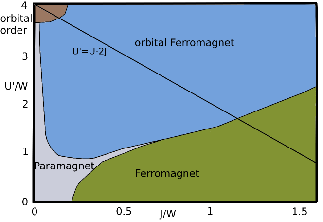
Figure 1: (color online) Schematic ground state phase diagram at quarter filling for $U/W=4$. The black line represents $U^{\prime}=U-2J$.

The ground state phase diagram consists of 4 different phases. For the case of both interaction parameters ($U^{\prime}$ and $J$) being small, there exists only a paramagnetic metallic phase. For small Hund’s coupling $J$ but large repulsive inter-orbital density-density interaction $U^{\prime}$, there appears an antiferro-orbitally ordered phase without spin polarization: Like for the Néel state of the antiferromagnet, the lattice exhibits a bipartite AB-structure, where electrons on the A-sites of the lattice only occupy the orbital $m=1$, while on the B-sites of the lattice they only occupy the orbital $m=2$. If, on the other hand, $U^{\prime}$ is kept small and the Hund’s coupling $J$ is increased, one encounters for $J/W\gtrsim 0.3$ a homogeneous ferromagnetic phase without orbital polarization. This ferromagnetic phase extends to a filling of approximately $n\approx 1.5$.Peters and Pruschke (2010) The bulk part of the phase diagram at quarter filling with $J>0$ and $U^{\prime}-J/2>0$ is, however, an anti-ferro orbitally ordered, ferromagnetic state. Thus, both types of order are quite obviously supporting each other. We should note here that for attractive inter-orbital interaction $U^{\prime}-J/2<0$ the energetically lowest state is a charge-density wave Peters and Pruschke (2010), which was however excluded in the phase-diagram Fig. 1. While the orbitally ordered state at $T=0$ always results in an insulating state, the homogeneous ferromagnetic state and the paramagnetic state both are metallic. We thus encounter a metal insulator transition (MIT) at $T=0$ when changing the interaction parameters.

It is well known that strong correlations tend to localize electrons at integer fillings Han et al. (1998); Koga et al. (2002); Pruschke and Bulla (2005); Koga et al. (2005); Werner et al. (2009) and that the transition point in the two-orbital Hubbard model depends on the strength of the Hund’s coupling $J$. deḾedici (2010) Furthermore, the localized electrons in the insulating region tend to form long range order. At quarter filling for the two-orbital Hubbard model on a bipartite lattice, this can be most efficiently be done by forming an orbital ordered ferromagnetic state, thus decreasing the energy of the system.

Comparing to paramagnetic results, the paramagnetic MIT occurs approximately at the same value of Hund’s coupling as this ferromagnetic MIT. However, the temperature scale of the paramagnetic MIT will be smaller, i.e. the paramagnetic MIT will be covered by ferromagnetic states having the lower energy for a bipartite lattice.

If this MIT will be observable in experiments is at least doubtful for two reasons. Firstly, it is not clear how one can experimentally change the inter-orbital interactions $J$ and $U^{\prime}$ without also significantly changing the Hubbard interaction $U$. Secondly, the neglected coupling to the lattice, which enhances the tendency towards orbital order due to Jahn-Teller-distortions, will quite likely cover this purely electronic effect. Nevertheless, it is important to realize that orbital order can be stabilized without resorting to lattice degrees of freedom by correlation effects only.

IV Influence of temperature

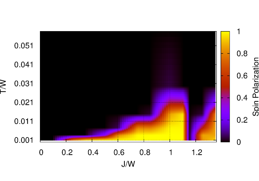
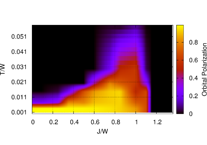
Figure 2: (color online) Spin polarization ($M=\sum_{m}(n_{m,\uparrow}-n_{m,\downarrow})$: upper panel) and orbital polarization ($P=\sum_{\sigma}(n_{1,\sigma}-n_{2,\sigma})$: lower panel) for different temperatures and Hund’s coupling at quarter filling and $U^{\prime}=U-2J$, $U=4W$. The dip at $J/W\approx 1.2$ in the magnetic polarization corresponds to the transition between the orbitally ordered ferromagnet for $J/W<1.2$ and the homogeneous ferromagnet for $J/W>1.2$.

Experimentally more relevant than changing the interaction parameters is the dependence of physical properties on temperature and magnetic field. In order to limit the number of parameters in our system, we will from now on focus on the special combination $U^{\prime}=U-2J$ for the interaction parameters, representing the SO(3) symmetry for isolated atoms Oleś (1983). Figure 2 shows the results for the spin and orbital polarization as function of temperature $T$ and Hund’s coupling $J$ in a false color plot. As we have only a limited number of actual data available, we used a polynomial fit to obtain a reasonably smooth density plot. Thus, the precise values and details of the transition lines should be regarded with some caution.

However, the temperature gap in the spin polarization at $J/W\approx 1.2$ is real and corresponds to the transition between orbitally ordered ferromagnetism for $J/W<1.2$ and homogeneous ferromagnetism (without orbital order) for $J/W>1.2$. In the former case, the ferromagnetic state is stabilized by orbital order induced by strong $U^{\prime}$, which is an insulator and consequently leads to the formation of local moments, which then order due to double exchange mechanism Zener (1951); Anderson and Hasegawa (1955); de Gennes (1960). For $J/W>1.2$ the orbital order has vanished (see lower panel of Fig. 2), but one still finds a ferromagnetic solution, however with reduced Curie temperature and magnetic moment. The magnetic state in this parameter region remains metallic and must therefore be characterized as itinerant ferromagnet stabilized mainly due to a gain in kinetic energy. These two rather different ferromagnetic phases are separated by a small region with a paramagnetic and orbitally disordered metal.

From Fig. 2 we have deduced the schematic phase diagram presented in Fig. 3. The black points in the graph correspond to the parameters, at which actual calculations have been performed.

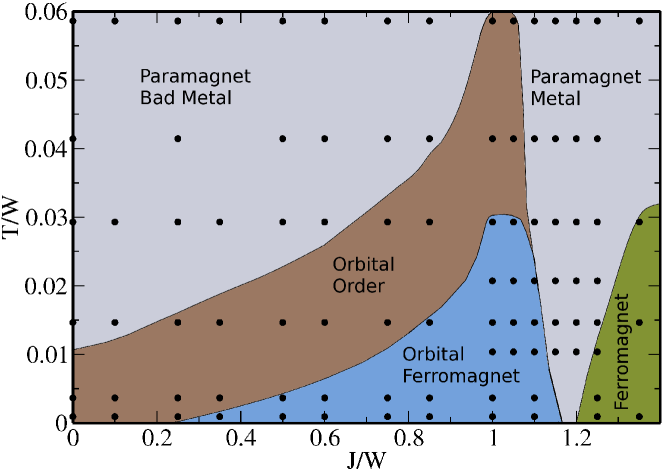
Figure 3: (color online) Schematic phase diagram for different temperatures and Hund’s coupling at quarter filling and $U^{\prime}=U-2J$, $U=4W$. The black points denote the parameters at which calculations have been performed and from which the phase boundaries were drawn.

The orbital order is mainly driven by the inter-orbital density-density interaction $U^{\prime}-J/2$. For small Hund’s coupling, meaning strong $U^{\prime}$, the transition temperature should behave like $T_{c}\sim 1/U^{\prime}$ in leading order from perturbation theory due to the same arguments as for the antiferromagnetic Néel state at half filling for large $U$. Increasing Hund’s coupling leads to a decreasing $U^{\prime}$ and vanishing orbital order. For $J>0$ and low temperatures the orbital order comes along with ferromagnetic order.

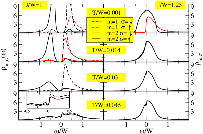
Figure 4: (color online) Left panels: Spectral functions within the orbitally ordered ferromagnetic region for $U=4W$, $J/W=1$. For decreasing temperatures a gap at the Fermi-energy $\omega=0$ is formed, and the spectral functions for $m=1$ and $m=2$ differ from each other. For temperatures below $T/W<0.02$ the orbitally ordered ferromagnetic state is stabilized. The inset in lowest panel shows a magnification around the Fermi energy clarifying the orbital order for this temperature. Right panels: Spectral functions for $J/W=1.25$. There is no difference in the spectral functions between $m=1$ and $m=2$. Additionally, the ferromagnetic transition temperature is much lower.

Up to now we have only discussed the static properties in the different phases, frequently referring to one case as an insulator, the other as a metal. To explain this distinction we discuss now the spectral functions for generic parameter values in the different cases. Figure 4 shows spectral functions corresponding to the cases $J/W<1.2$ (left panels) and $J/W>1.2$ (right panels). As already observed for the order parameters, one first finds orbital order with decreasing temperature for $J/W<1.2$, and a second transition to a ferromagnet for even lower temperatures. In the case $J/W>1.2$, on the other hand, there is no sign for orbital ordering, but a clear ferromagnetic polarization of the spectra for the lowest shown temperature. The spectral functions of both systems differ very strongly. The orbitally ordered system exhibits characteristic van Hove singularities due to the reduced translational symmetry, and a gap at the Fermi energy $\omega=0$, thus being an insulator. The system without orbital order does not show this gap, but a smooth and finite DOS at the Fermi energy, thus being metallic.

However, the insulating behavior for $J/W<1.2$ is not only due to orbital order, resulting in a doubling of the unit cell. The gap can also be found above the critical temperature of the phase transition, see Fig. 5. This figure shows spectral functions for $T/W=0.08$ in the paramagnetic phase for different values of the Hund’s coupling. By increasing the Hund’s coupling the gap is closed and a broad peak is formed. At this temperature, there is no sharp phase transition between the insulator and the metal, but a crossover between both phases. One can argue that the gap is formed by the strong inter-orbital density-density interaction. This emphasizes the importance of taking into account the orbital level structure of Transition Metal Oxides when modeling their properties, like the well-known metal insulator transition in V₂O₃ Imada et al. (1998).

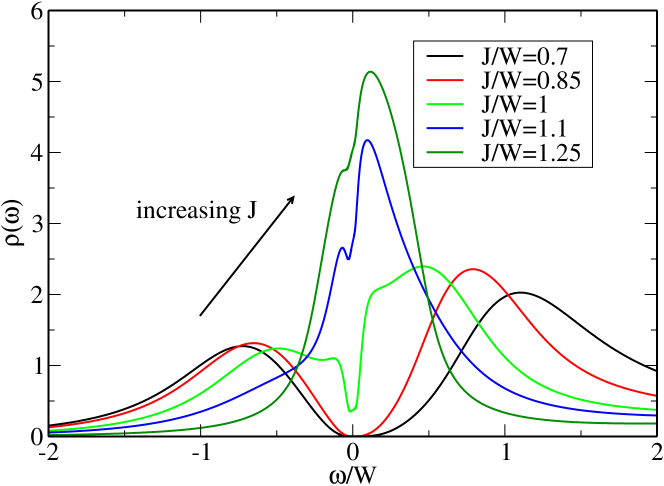
Figure 5: (color online) Spectral functions for $U=4W$, $T/W=0.08$, $U^{\prime}=U-2J$, and different $J$. For all shown spectral functions the system is in a paramagnetic state. For increasing $J$, the gap at the Fermi-energy $\omega=0$ vanishes.

V Magnetoresistance

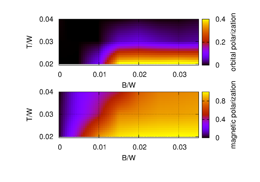
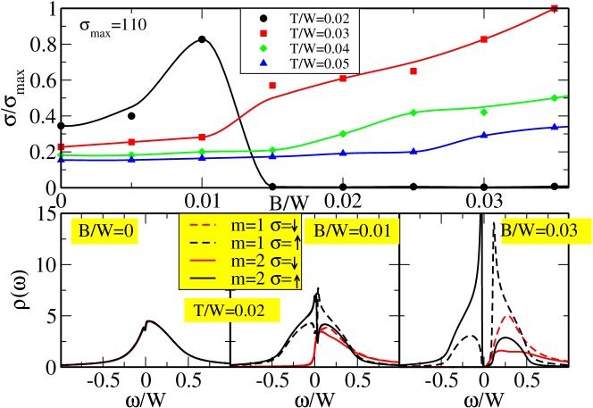
Figure 6: (color online) Response of the system to an applied magnetic field at $U/W=4$, $J/W=1.2$, $U^{\prime}=U-2J$. The upper two panels show the magnetic and orbital polarization for different temperatures $T/W$ and magnetic fields $B/W$. The lower panels show the conductivity $\sigma$ scaled by $\sigma_{max}=110$ (compare $\sigma_{max}$ with Fig. 7) for $4$ different temperatures (lines are meant as guide to the eye), and the spectral functions at $T/W=0.02$.

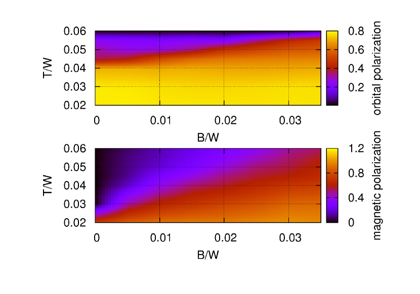
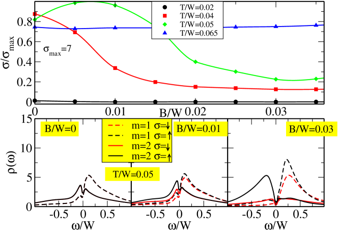
Figure 7: (color online) Response of the system to an applied magnetic field at $U/W=4$, $J/W=1.05$, $U^{\prime}=U-2J$. The upper two panels show the magnetic and orbital polarization for different temperatures $T/W$ and magnetic fields $B/W$. The lower panels show the conductivity $\sigma$ scaled by $\sigma_{max}=7$ for $4$ different temperatures (lines are meant as guide to the eye), and the spectral functions at $T/W=0.05$.

Besides temperature, also the magnetic field can be varied very easily in experiments. An increasing magnetic field will enhance the magnetic polarization of the system. However, especially in the vicinity of the phase transition $J/W\approx 1.2$, where the orbitally ordered ferromagnetic state has disappeared, it is a priori not clear how the ferromagnetic state will look like. When applying a magnetic field within the paramagnetic phase between both ferromagnetic phases, the system can form either an orbitally ordered or an orbitally homogeneous state. Both states do considerably differ in their physical properties, as the orbitally ordered state is gapped at the Fermi energy, while the homogeneous state is not.

In Figs. 6 and 7 we analyze the conductivity of the system for different temperatures and magnetic fields. The conductivity can be easily calculated within the DMFT, as the self-energy is purely local. We here must take care of a possible AB-ordering (Néel order) in the orbital index. The conductivity at $\omega=0$ can be written as Pruschke and Zitzler (2003)

$$\sigma(\omega=0) = c\sum_{\sigma,m}\int_{-\infty}^{\infty}d\epsilon\langle v^{2}\rangle(\epsilon)\int_{-\infty}^{\infty}d\omega^{\prime}\frac{df(\omega^{\prime})}{d\omega^{\prime}}$$

$$\cdot\bigl{[}A^{\mathcal{A}}_{m,\sigma}(\epsilon,\omega^{\prime})A^{\mathcal{B}}_{m,\sigma}(\epsilon,\omega^{\prime})+B_{m,\sigma}(\epsilon,\omega^{\prime})^{2}\Bigr{]}$$

$$A^{\mathcal{S}}_{m,\sigma}(\epsilon,\omega^{\prime}) = -\frac{1}{\pi}\mathfrak{Im}\Bigl{(}\frac{\zeta^{\mathcal{\bar{S}}}_{m,\sigma}}{\zeta^{\mathcal{A}}_{m,\sigma}\zeta^{\mathcal{B}}_{m,\sigma}-\epsilon^{2}}\Bigr{)}$$

$$B_{m,\sigma}(\epsilon,\omega^{\prime}) = -\frac{1}{\pi}\mathfrak{Im}\Bigl{(}\frac{\epsilon}{\zeta^{\mathcal{A}}_{m,\sigma}\zeta^{\mathcal{B}}_{m,\sigma}-\epsilon^{2}}\Bigr{)}$$

$$\zeta^{\mathcal{S}}_{m,\sigma} = \omega^{\prime}+\mu-\Sigma_{m,\sigma}^{\mathcal{S}}(\omega^{\prime}),$$

where $A_{m,\sigma}(\epsilon,\omega^{\prime})$ and $B_{m,\sigma}(\epsilon,\omega^{\prime})$ are the diagonal and off-diagonal Green’s functions of the AB-lattice respectively, $f(\omega^{\prime})$ is the Fermi-function, $\mu$ the chemical potential, $\Sigma^{\mathcal{S}}_{m,\sigma}(\omega^{\prime})$ the local self-energy. $\mathcal{S}=(\mathcal{A},\mathcal{B})$ corresponds to the sub-lattice, for which $\mathcal{\bar{A}}=\mathcal{B}$ holds. Finally, $\langle v^{2}\rangle(\epsilon)$ is the averaged squared Fermi-velocity, in which the lattice structure enters Bluemer and van Dongen (2003). The prefactor $c=\frac{e^{2}}{h}\frac{\pi^{2}}{a}$ consists of the resistance quantum and a non-universal part, depending on the details of the lattice. In the following, we use c=1 for convenience.

Figure 6 summarizes the properties of the system for $J/W=1.2$. The upper two panels of the figure show the magnetic and orbital polarization, while the lower panel shows conductivity and spectral functions for different temperatures $T$ and magnetic fields $B$. These parameters correspond to the minimum of the Curie-temperature (dip) in Fig. 3, where there is neither orbital nor magnetic order for $B=0$. We discuss the conductivity instead of the resistivity here as we expect a MIT at some point, leading to a drop to zero in $\sigma$, which is easier to visualize than a divergence in $\rho$.

If one applies a magnetic field at low temperatures, $T/W\approx 0.02$, both spin and orbital polarizations are induced. Assuming a bandwidth of $W=1eV$, this corresponds to a temperature of $T\approx 240K$. The system can still gain more energy by localizing the electrons on different orbitals in the presence of a magnetic field. This magnetoresistance effect corresponds to a MIT triggered by applying a magnetic field. Furthermore, these results agree with the fact that applying a magnetic field at low temperatures near a MIT in a one-band model favors the insulating solution Laloux et al. (1994). Looking at the spectral functions for $B/W=0.01$, the middle of the lower panels in the figure, a spin polarized state has formed. Nevertheless, all spectral functions still have spectral weight at the Fermi energy. The majority-spin spectral functions form a two peak structure, firstly even increasing the weight at the Fermi energy. Further increasing the magnetic field above $B/W>0.015$ (right part of lower panel) stabilizes the usual orbitally ordered ferromagnetic state with a gap at the Fermi energy.

This behavior is reflected in the conductivity, which directly depends on the spectral weight at the Fermi energy. With increasing magnetic field the conductivity initially increases at low temperatures, but then drops to zero as the gap opens. If one further decreases the temperature, the initial conductivity increase for small magnetic fields will be more pronounced, but it again eventually drops to zero for magnetic fields of approximately $B/W\approx 0.015$. Thus, at low temperatures, one observes a rather dramatic magnetoresistance effect as function of magnetic field, reminiscent of the colossal magnetoresistance effect in the manganites.

For higher temperatures the situation is different. In this case, no orbital polarization is stabilized, and no gap is formed at the Fermi energy. Increasing the magnetic field causes the conductivity to increase smoothly, as the spectral weight of the majority spin at the Fermi energy is increased.

Let us compare these results with those for $J/W=1.05$ collected in Fig. 7 . For this value of $J$, the orbital order has its highest transition temperature. Nevertheless, for temperatures of approximately the transition temperature, the spectral function is non-zero at the Fermi energy, even in the orbitally ordered state. To compare the conductivity in Figs. 6 and 7 properly, one should also compare the scaling constants $\sigma_{max}$. Increasing $J$ leads to a more pronounced peak at the Fermi energy in the spectral function. This is reflected in $\sigma_{max}$, which for $J/W=1.2$ takes the value $\sigma_{max}=110$ (in arbitrary units, neglecting the constant factors $c$ for calculating the conductivity, which is the same in both cases), while for the orbitally ordered ferromagnetic ground state the scaling constant is $\sigma_{max}=7$.

Increasing the temperature without applying a magnetic field, leads first to a vanishing spin polarization and later, at temperatures $T/W\approx 0.05$, to a paramagnetic state. For $T/W<0.04$ the system is gapped and the conductivity is nearly zero. Approaching now the transition temperature of the orbitally ordered phase, spectral weight is shifted to the Fermi energy. At this point, a magnetic field leads again to an increase of the gap width and to a stabilization of the orbital order. The corresponding temperature for the magnetoresistance-effect is $T\approx 600K$, again assuming a bandwidth $W=1eV$.

This behavior can be seen in the upper panels of Fig. 7 in which the transition temperature of the orbital order increases with increasing magnetic field, and in the lower panels directly for the spectral functions or for the conductivity. For $T/W\approx 0.05$, the latter now again shows a maximum at some small magnetic field, decreasing again with increasing magnetic field. However, compared to the case $J/W\approx 1.2$, the effect here is less dramatic. For even higher temperatures, neither an orbital polarization nor a gap at the Fermi energy is induced by a magnetic field resulting in a nearly constant conductivity.

One can do similar calculations for smaller Hund’s coupling $J/W<1$ or larger $J/W>1.25$. For smaller Hund’s coupling the system is in an insulating state even for temperatures above the critical temperature for the ordered phases. Applying magnetic fields will also increase the transition temperature of the orbitally ordered phase, but as the system is already gapped in the paramagnetic state, the conductivity will not change significantly. For larger Hund’s coupling, applying a magnetic field will not induce orbital order anymore. The system will stay in a metallic state with a correspondingly smooth and weak variation of the physical properties.

VI Conclusions

We have analyzed the properties of the two-orbital Hubbard model at quarter filling for a range of temperatures and magnetic fields. As expected, ferromagnetic order is prevalent at quarter filling, but depending on the ratio of inter-orbital interaction and Hund’s exchange, it can appear either without or with accompanying orbital order.

Our calculations show that orbital order can be stabilized without including Jahn-Teller distortions,Leonov et al. (2008) and it is stabilized by a strong inter-orbital density-density interaction. If one decreases the strength of this interaction, the orbital order will eventually vanish. As a result a metal insulator transition can be found, which can also be triggered by applying a magnetic field close to the transition. This gives rise to a very strong magnetoresistance effect, as one can drive the system from a metallic into an insulating state. The strength of this magnetoresistance effect depends sensitively on the Hund’s coupling $J$. In particular, we found a critical regime for $J$ between an orbitally ordered ferromagnet and an orbitally homogeneous one, where a particularly strong magnetoresistance effect exists. Note that these interaction values for this particularly interesting behavior, $U/W=4$ and $J/W=1.2$, are not completely unrealistic for Transition Metal Oxides. It therefore might be interesting to look for $e_{g}$ systems at quarter filling which are in this parameter regime if they exhibit strong magnetoresistance.

Another rather amusing fact is that we found an insulating paramagnetic state for strong inter-orbital density-density interaction reaching to temperatures far above the long-range ordered phases. This shows the importance of the orbital level structure when analyzing the metal insulator transition in, for example, V₂O₃.