Forming Protostars in Molecular Clouds with
Shocked Envelope Expansion and Core Collapse

Abstract

Spectral observations of molecular line profiles reveal the so-called ‘blue profiles’ for double-peaked molecular lines with stronger blue and weaker red peaks as notable features for star-forming cloud core collapses under the self-gravity. In contrast, $\sim 25-30$ per cent of observed molecular spectral line profiles in star-forming clouds or cores also show the so-called double-peaked ‘red profiles’ with red peaks stronger than blue peaks. Gao & Lou (2010) show that these unexplained ‘red profiles’ can be signatures of global dynamics for envelope expansion with core collapse (EECC) within star-forming molecular clouds or cores. We demonstrate here that spatially-resolved ‘red profiles’ of HCO⁺ (J$=1-0$) and CS (J$=2-1$) molecular transitions from the low-mass star-forming cloud core FeSt 1-457 together with its radial profile of column density inferred from dust extinction observations appear to reveal a self-similar hydrodynamic shock phase for global EECC. Observed spectral profiles of C¹⁸O (J$=1-0$) are also fitted by the same EECC model. For further observational tests, the spatially-resolved profiles of molecular transitions HCO⁺ (J$=3-2$) and CS (J$=3-2$) as well as the radial profiles of (sub)millimetre continuum emissions at three wavelengths of 1.2mm, 0.85mm and 0.45mm from FeSt 1-457 are also predicted.

1 Introduction

Gravitational collapses of molecular clouds and cloud cores lead to early formation of protostars therein (e.g. Shu, 1977; Shu, Adams & Lizano, 1987; McLaughlin & Pudritz, 1997; McKee & Tan, 2002). For starless and star-forming molecular cloud cores in early phases, the central dense mass blob might not involve discs or outflows especially for those grossly spherical molecular clouds. Recent theoretical development of self-similar hydrodynamic shock models involving the self-gravity reveals, among others, a novel plausible dynamic scenario of global envelope expansion with core collapse (EECC) (Lou & Shen, 2004; Bian & Lou, 2005; Lou & Gao, 2006; Wang & Lou, 2008) with an expanding infall radius $R_{\rm inf}$ during early dynamic evolution stages of forming protostellar cores. Together with other pertinent yet independent diagnostics and constraints, observations of various molecular emission spectral line profiles, especially those with high enough spatial and frequency resolutions and/or different line transitions of the same molecules, make it possible to identify the gross hydrodynamic and thermodynamic structures of star-forming molecular clouds with grossly spherical morphologies.

Major diagnostics to probe molecular cloud structures include spatially-resolved spectral profiles for various molecular line transitions (e.g. Zhou et al., 1993; Tafalla et al., 2006, Fu, Gao & Lou 2010), radial profiles of column densities inferred from dust extinctions of background stars behind a molecular cloud (e.g. Alves et al. 2001; Kandori et al., 2005), radial profiles of (sub)millimetre continuum emissions (e.g. Shirley et al., 2000; Motte & André, 2001) etc. Any of such separate observational diagnostics may be fitted with empirical and parametrized models on an individual basis to various extents as can be found in the literature. In contrast and in order to remove potential model degeneracies, our strategy is to constrain the underlying cloud model using the hydrodynamics and by all available observational data simultaneously. We also make model predictions for specific observational tests. We mainly focus on those molecular clouds which appear grossly spherical as our spherically symmetric hydrodynamics represents a first-order approximation in that direction. For illustration, we choose the molecular cloud core FeSt 1-457 for specific observational comparisons. We also summarize the main results of our model comparisons with several observations for another star-forming cloud core L1517B as supporting evidence.

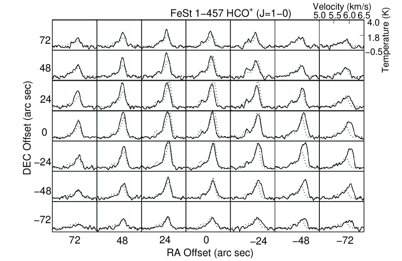
Figure 1: The observed molecular line transition HCO⁺ (J$=1-0$) in a spatially-resolved grid-map of star-forming molecular cloud core FeSt 1-457 (solid line profiles) superposed with our best-fit EECC shock dynamic model results (dotted line profiles). The receding velocity of the entire cloud core FeSt 1-457 along the line of sight is estimated to be $\sim 5.75$ km s^-1. Each grid has the local receding velocity along the line of sight as the abscissa and antenna temperature as the ordinate (see the very upper right grid as a sample). The observational data map of Aguti et al. (2007) is centered at right ascension $\alpha_{J2000}=17^{\rm h}35^{\rm m}47.5^{\rm s}$ and declination $\delta_{J2000}=-25^{\circ}33^{\prime}2.0^{\prime\prime}$, with a grid spacing of $\sim 24^{\prime\prime}$ (corresponding to $\sim 3.0\times 10^{3}$ au at a distance of $\sim 130$ pc for the Pipe Nebula) and a maximum observed area of $168^{\prime\prime}\times 168^{\prime\prime}$ in the plane of the sky. Molecular spectral line profile fittings are based on our general polytropic EECC shock model (Wang & Lou, 2008; Gao & Lou, 2010), by adopting a step function molecular abundance profile (see details in Table 1) and by performing the RATRAN computation. Our model spectral line profiles are convolved with the beam width of $\sim 24^{\prime\prime}$ and multiplied by an IRAM 30m telescope mean beam efficiency of $\sim 0.75$.

Regarding the molecular line diagnostics, there are two major asymmetric double-peak molecular spectral line profiles oft-observed in star-forming clouds, viz., the so-called ‘blue profiles’ with stronger blue-shifted peaks than red-shifted peaks and the so-called ‘red profiles’ with stronger red-shifted peaks than blue-shifted peaks. The level of such spectral line profile asymmetries can change in a gradual manner for spatially-resolved observations. While the observed ‘blue profiles’ of molecular spectral lines are modelled and generally interpreted as characteristic signatures of radial infalls in molecular clouds (Zhou et al., 1993; Gao, Lou & Wu, 2009), the somewhat ignored yet wide presence of unexplained ‘red profiles’ (e.g. Mardones et al., 1997; Evans, 2003; Velusamy et al., 2008) remains a conceptual gap in our understanding of star-forming molecular cloud dynamics. Moreover, sometimes ‘blue profiles’ and ‘red profiles’ coexist in molecular cloud cores for the same line transition (e.g. Tafalla et al., 2000), and/or for different line transitions (e.g. Tafalla et al., 2006). For the possible interpretation of ‘red profiles’ of molecular spectral lines alone, one may think of several mechanisms, e.g. rotations (e.g. Di Francesco et al., 2001), bipolar outflows inclined close to the plane of the sky (e.g. Fiege & Henriksen, 1996), turbulence (e.g. Ossenkopf, 2002) and thermal pulsations (e.g. Lada et al., 2003).

For FeSt 1-457 (see Fig. 1), disc rotation is unlikely, as this cloud core is most likely evolving in an early phase. A global cloud core rotation of FeSt 1-457 may be excluded by spatially-resolved spectral line observations; i.e., the currently data do not show such evidence. At present, these mechanisms just mentioned have not been shown to also account for cloud density profiles and radial profiles of (sub)millimetre continuum emissions simultaneously within a consistent model framework. Alternatively, it was suggested that ‘red profiles’ in certain star-forming sources may be caused by clouds involving EECC (Lou & Shen, 2004; Thompson & White, 2004). It is thus crucial to reproduce the observed ‘red profiles’ using our general polytropic EECC shock models via radiative transfer calculations (Gao & Lou, 2010). Meanwhile, we require the model density profile to be consistent with the observational inference of dust extinctions and further predict other spectral line profiles as well as radial profiles of (sub)millimetre continuum emissions as future observational tests.

Four main contributions of our model analysis in this paper are as follows. First, for the grossly spherical molecular cloud core FeSt 1-457, we construct a self-similar general polytropic hydrodynamic EECC shock model (Lou & Shen, 2004; Lou & Gao, 2006; Wang & Lou, 2008), and radiative transfer calculations are performed to reproduce the observed ‘red profiles’ and other spectral profiles of molecular transition lines in the cloud core. Secondly, we advance the conceptual framework of constraining the molecular cloud dynamics using several available diagnostics simultaneously in order to solve this challenging issue in molecular astronomy. For FeSt 1-457, the column density profile of our EECC shock dynamics is also sensibly fitted with the observationally inferred column density profile by the dust extinction data (e.g. Kandori et al., 2005). Thirdly, while no data for (sub)millimetre continua are available for FeSt 1-457 at present, for scenario consistency and further observational tests, we predict radio continuum emissions at three wavelengths of 1.2 mm, 0.85 mm and 0.45 mm. For the same reason, the spatially-resolved spectral profiles of molecular line transitions HCO⁺ (J$=3-2$) and CS (J$=3-2$) are also predicted for observational tests. Finally, we suggest (Gao & Lou, 2010) that such EECC shock phase may evolve from damped nonlinear radial pulsations of molecular cloud core within one or two cycles. Corresponding to different phases of such damped large-scale radial pulsations, different dynamic phases may give rise to distinct diagnostics.

2 Star-Forming Molecular
    Cloud Core FeSt 1-457

As a chosen candidate, the molecular cloud core FeSt 1-457 appears to be a grossly spherical dark globule in the Pipe Nebula at a distance of $\sim 130$ pc away (e.g. Lombardi et al. 2006). Without detecting a star, this starless cloud core in the early phase of protostar formation has a diameter of $\sim 35,000$ au with an angular diameter $\sim 4.5^{\prime}$ derived from the optical images (e.g. Aguti et al., 2007). The spectral data from Aguti et al. (2007) for spatially-resolved spectral line profiles of three molecular transitions HCO⁺ (J$=1-0$), CS (J$=2-1$) and C¹⁸O (J$=1-0$) (Figs. 1 and 4) were acquired in 2003 by the 30-metre millimetre-wave telescope of Institut de Radioastronomie Millimétrique (IRAM) on Pico Veleta near Granada in Spain. The spatial resolution of this spectral data set is $\sim 24^{\prime\prime}$ for the beam width in the frequency band $90-110$ GHz with a mean beam efficiency of $\sim 0.75$ at uncertainties $\;\lower 4.0pt\hbox{${\buildrel\displaystyle<\over{\sim}}$}\;4$ per cent (e.g. Greve et al. 1998). The dust extinction data of FeSt 1-457 for the inferred radial profile of column density with a $\sim 30^{\prime\prime}$ beam resolution are also available together with error bars (e.g. Kandori et al., 2005, and see the upper panel of our Fig. 6).

Global expansions in the outer layer or envelope of this globule are hinted by asymmetric molecular spectral line profiles and cloud oscillations were proposed to be the origin of such expansions (e.g. Aguti et al., 2007). In our advocated scenario, such large-scale nonlinear cloud radial pulsations cannot persist forever but may initiate core collapses and envelope expansions within one or two cycles and hence may lead to a self-similar EECC shock phase (Lou & Gao, 2006; Gao & Lou, 2010). We demonstrate that the global EECC shock phase seem to persist in FeSt 1-457 by molecular spectral line profile fits using the spherically symmetric general polytropic self-similar dynamic model (Wang & Lou, 2008). Meanwhile, we also use the dust extinction data (Kandori et al., 2005) of FeSt 1-457 for the radial profile of column density with a $\sim 30^{\prime\prime}$ beam resolution to constrain our EECC shock hydrodynamics (Fig. 6). Finally for future observational tests, we predict the spatially-resolved spectral profiles of molecular line transitions HCO⁺ (J$=3-2$) and CS (J$=3-2$) as well as three radial profiles of millimetre continua at wavelengths 1.2mm, 0.85mm and 0.45mm with estimated error ranges using the density and temperature profiles of the same underlying EECC shock dynamics (Fig. 5 and 6), as have been already detected in other protostar-forming molecular cloud cores (e.g. Shirley et al., 2002).

3 EECC Shock Hydrodynamics and Formation of Red Profiles for Molecular Spectral Lines

3.1 Self-similar Hydrodynamic Models
   and EECC Shock Solutions

EECC self-similar hydrodynamic shock solutions have been investigated with different equations of state (EoS) in recent years (Lou & Shen, 2004; Lou & Gao, 2006; Wang & Lou, 2008). We here adapt the magnetohydrodynamic (MHD) model formulation with general polytropic EoS in Wang & Lou (2008) but without the magnetic field (i.e. setting the magnetic field parameter $h=0$ in that paper).

Our model formulation begins with the ideal hydrodynamic partial differential equations (PDEs) for a spherically symmetric molecular cloud in spherical polar coordinates $(r,\ \theta,\ \phi)$, namely

$${{\partial\rho}\over{\partial t}}+{1\over{r^{2}}}{{\partial}\over{\partial r}}(r^{2}\rho u)=0\ ,$$ (1)

$${{\partial u}\over{\partial t}}+u{{\partial u}\over{\partial r}}=-{1\over{\rho}}{{\partial p}\over{\partial r}}-{{GM}\over{r^{2}}}\ ,$$ (2)

$${{\partial M}\over{\partial t}}+u{{\partial M}\over{\partial r}}=0\ ,\qquad\qquad\qquad{{\partial M}\over{\partial r}}=4\pi r^{2}\rho\ ,$$ (3)

$$\left(\frac{\partial}{\partial t}+u\frac{\partial}{\partial r}\right)\left({\rm ln}\frac{p}{\rho^{\gamma}}\right)=0\ ,$$ (4)

where, as functions of both radius $r$ and time $t$, dependent variables $u$, $\rho$, $M$, and $p$ are the radial flow velocity, mass density, enclosed mass within radius $r$ at time $t$ and thermal gas pressure, respectively; $G$ is the gravitational constant and $\gamma$ is the polytropic index. These nonlinear hydrodynamic PDEs describe the conservations of mass (eq (1)), radial momentum (eq (2)) and specific entropy along streamlines (eq (4)).

Self-similar solutions to nonlinear PDEs (1)$-$(4) by the following self-similar transformation can be constructed, namely

$$r=k^{1/2}t^{n}x\ ,$$ (5)

$$u=k^{1/2}t^{n-1}v(x)\ ,\qquad\qquad\rho=\frac{\alpha(x)}{4\pi Gt^{2}}\ ,$$ (6)

$$M=\frac{k^{3/2}t^{3n-2}m(x)}{(3n-2)G}\ ,\qquad p=\frac{kt^{2n-4}\alpha(x)^{\gamma}m(x)^{q}}{4\pi G}\ ,\$$ (7)

where $x$ is the self-similar independent variable combining $r$ and $t$ in a special manner, and $v(x)$, $\alpha(x)$ and $m(x)$ are functions of $x$ only and represent the dimensionless reduced radial flow velocity, mass density and enclosed mass, respectively; and $n$ and $\gamma$ in these self-similar transformations are two additional scaling indices allowed, with the algebraic relation $q=2(n+\gamma-2)/(3n-2)$. Here $k$ is a parameter related to the sound speed within the molecular cloud. Physically, a positive enclosed mass $M$ requires the inequality $n>2/3$ in the similarity transformation above. For $n+\gamma=2$ and thus $q=0$ as in this paper unless otherwise stated, we reduce to the conventional polytropic hydrodynamics (Wang & Lou, 2007, 2008) as an important subcase. Other important physical variables, namely the gas thermal temperature (invoking the ideal gas law) and the central mass accretion rate in the molecular cloud centre are

$$T\equiv\frac{p}{k_{\rm B}\rho/(\mu m_{\rm H})}=\frac{\mu m_{\rm H}}{k_{B}}kt^{2(n-1)}\alpha(x)^{\gamma-1}m(x)^{q}\ ,$$ (8)

$$\dot{M_{0}}=k^{3/2}t^{3(n-1)}m_{0}/G\ ,$$ (9)

respectively. Here $m_{0}\equiv m(0)$ is the reduced central enclosed mass, $k_{\rm B}$ is Boltzmann’s constant, $m_{\rm H}$ is the atomic hydrogen mass, and $\mu$ is the mean molecular weight setting to be 2 in our model analysis for star-forming gas cloud consisting mainly of molecular hydrogen H₂.

By adopting self-similar transformation equations (5)$-$(7), nonlinear hydrodynamic PDEs (1)$-$(4) can be readily cast into two coupled nonlinear ordinary differential equations (ODEs) which can be solved by a combination of analytical and numerical techniques (see, e.g. Wang & Lou, 2008). These two coupled nonlinear ODEs are

$$\bigg{[}\bigg{(}2-n+\frac{3n-2}{2}q\bigg{)}\alpha^{1-n+\frac{3nq}{2}}x^{2q}(nx-v)^{q}-(nx-v)^{2}\bigg{]}$$

$$\times\frac{d\alpha}{dx}=2\frac{(x-v)}{x}\alpha\bigg{[}(nx-v)+q\alpha^{1-n+\frac{3nq}{2}}x^{2q}(nx-v)^{q-1}\bigg{]}$$

$$-\alpha\bigg{[}(n-1)v+\frac{(nx-v)}{(3n-2)}\alpha\qquad\qquad\qquad\qquad\qquad\qquad$$

$$+q\alpha^{1-n+\frac{3nq}{2}}x^{2q-1}(nx-v)^{q-1}(3nx-2v)\bigg{]}\ ,\qquad$$ (10)

$$\bigg{[}\bigg{(}2-n+\frac{3n-2}{2}q\bigg{)}\alpha^{1-n+\frac{3nq}{2}}x^{2q}(nx-v)^{q}-(nx-v)^{2}\bigg{]}$$

$$\times\frac{dv}{dx}=2\frac{(x-v)}{x}\bigg{(}2-n+\frac{3nq}{2}\bigg{)}\alpha^{1-n+\frac{3nq}{2}}x^{2q}(nx-v)^{q}$$

$$-(nx-v)\bigg{[}(n-1)v+\frac{(nx-v)}{(3n-2)}\alpha\qquad\qquad\qquad$$

$$+q\alpha^{1-n+\frac{3nq}{2}}x^{2q-1}(nx-v)^{q-1}(3nx-2v)\bigg{]}\ .$$ (11)

In the above mathematical derivations, we also make use of the following algebraic relation

$$m=\alpha x^{2}(nx-v)\$$ (12)

from the mass conservation (1) and (3). Once $\alpha(x)$ and $v(x)$ are known, we then readily obtain the reduced enclosed mass $m(x)$. Two sets of analytical asymptotic similarity solutions for $x\rightarrow+\infty$ and $x\rightarrow 0^{+}$ respectively serve as the boundary conditions in solving two coupled nonlinear ODEs (10) and (11). Among other possible solutions, we have for the $x\rightarrow+\infty$ regime

$$\alpha=Ax^{-{2}/{n}},\qquad\qquad\qquad\qquad\qquad\qquad\qquad\qquad\qquad$$

$$v=\bigg{[}-\frac{nA}{(3n-2)}+2(2-n)n^{q-1}A^{1-n+3nq/2}\bigg{]}x^{{(n-2)}/{n}}$$

$$+Bx^{{(n-1)}/{n}}\ ,$$ (13)

and for the $x\rightarrow 0^{+}$ regime, the central free-fall solution

$$v=-\bigg{[}\frac{2m_{0}}{(3n-2)x}\bigg{]}^{1/2}\ ,\qquad\ \ \alpha=\bigg{[}\frac{(3n-2)m_{0}}{2x^{3}}\bigg{]}^{1/2}\ .$$ (14)

Here, the mass parameter $A$ and the velocity parameter $B$, describing the asymptotic boundary condition as $x\rightarrow+\infty$, are two constants of integration and are important parameters to characterize the global self-similar dynamic solution. Meanwhile, the reduced enclosed mass $m_{0}\equiv m(0)$ describes the central point mass embedded deep in the cloud core. Then our global self-similar dynamic solutions can be constructed by straightforward numerical integrations using the standard fourth-order Runge-Kutta scheme and by specifying boundary conditions (13) and (14). In the absence of a shock, $A$ and $B$ are specified and $m_{0}$ is determined accordingly; i.e. only two are independent among the three parameters. For solutions with shocks, the shock location is another parameter and discontinuity across a shock front is introduced; global solutions can be still constructed by simply requiring the conservation laws of mass, radial momentum and energy across the upstream and downstream sides of the shock front (see Wang & Lou (2008) for more details regarding the hydrodynamic formulation).

3.2 The EECC hydrodynamic Shock Solution
  Adopted for the Cloud Core FeSt 1-457

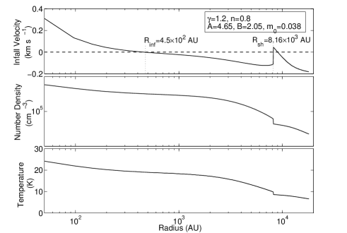
Figure 2: Radial profiles of infall speed $-u(r,\ t)$, H₂ number density $N(r,\ t)$ and thermal temperature $T(r,\ t)$ for the polytropic EECC shock dynamic phase of a model cloud for FeSt 1-457 with an evolutionary timescale $t\sim 2.8\times 10^{5}$ yr. This EECC shock dynamic model has an expanding infall radius $R_{\rm inf}=4.5\times 10^{2}$ au (top panel), a shock radius $R_{\rm sh}=8.16\times 10^{3}$ au (all three panels) and an outer cloud boundary of $R_{\rm out}=1.80\times 10^{4}$ au. The infall radius $R_{\rm inf}$ and shock radius $R_{\rm sh}$ expand at speeds of $\sim 0.015~{}{\rm km~{}s^{-1}}$ and $\sim 0.27~{}{\rm km~{}s^{-1}}$, respectively. The top panel shows that the cloud core collapses inside $R_{\rm inf}$ while the envelope outside $R_{\rm inf}$ expands outwards with typical gas flow speeds $\;\lower 4.0pt\hbox{${\buildrel\displaystyle<\over{\sim}}$}\;0.1~{}{\rm km~{}s^{-1}}$. The middle and bottom panels show a number density increase by a factor $\sim 10^{3}$ and a temperature increase by a factor $\;\lower 4.0pt\hbox{${\buildrel\displaystyle>\over{\sim}}$}\;3$ times towards the core centre where a point mass blob of $M_{0}=0.0202M_{\odot}$ resides.

In our model analysis, various EECC shock dynamic solutions are extensively explored in order to plausibly represent the dynamic state of FeSt 1-457 by adopting model fitting procedures detailed in Section 4. Finally after an extensive search, a sample EECC shock dynamic solution with polytropic index $\gamma=1.2$, scaling parameter $n=0.8$ and three coefficients of asymptotic conditions $A=4.65$, $B=2.05$ and $m_{0}=0.038$ is chosen to fit the molecular spectral line profile data and the column density radial profile inferred from dust extinction observations. Two relevant physical scalings (see subsection 2.3 of Gao & Lou, 2010) of the length scale and number density scale are specifically chosen below as

$$k^{1/2}t^{n}=4.8\times 10^{3}~{}{\rm au}\ ,$$ (15)

$$(4\pi G\mu m_{\rm H}t^{2})^{-1}=2.7\times 10^{4}~{}{\rm cm^{-3}}\ ,$$ (16)

with the mean molecular weight $\mu=2$.

Our EECC hydrodynamic shock solution offers the global radial structural profiles of radial infall velocity $u(r,\ t)$, number density $N(r,\ t)$ and thermal gas temperature $T(r,\ t)$ (see Fig. 2); the cloud temperature $T(r,\ t)$ increases towards the centre and an infall radius $R_{\rm inf}=4.5\times 10^{2}~{}{\rm au}$ expanding at a speed of $\sim 0.015~{}{\rm km~{}s^{-1}}$ separates the inner core collapse domain ($u<0$) and the outer envelope expansion domain ($u>0$). An outgoing spherical shock is at radius $R_{\rm sh}=8.16\times 10^{3}$ au with a shock travelling speed of $\sim 0.27~{}{\rm km~{}s^{-1}}$ and the outer cloud core radius is at $R_{\rm out}=1.80\times 10^{4}$ au. Following the chosen scales by expressions (15) and (16), the sound parameter $k$ values across a shock front are different; the upstream (pre-shock) side has $k^{1/2}=k_{\rm u}^{1/2}=48.7~{}{\rm km~{}s^{-0.8}}$ and the downstream (post-shock) side has $k^{1/2}=k_{\rm d}^{1/2}=49.1~{}{\rm km~{}s^{-0.8}}$. Correspondingly (also as a result of different densities in the upstream and downstream sides, see eq. (8) in Lou & Gao 2006), the sound speed $c$ across the outgoing shock front is different: $c_{\rm u}=0.133~{}{\rm km\ s}^{-1}$ and $c_{\rm d}=0.143~{}{\rm km\ s}^{-1}$. This EECC shock dynamic model describes a molecular cloud core in the early phase of star formation (a timescale of $t\sim 2.8\times 10^{5}~{}{\rm yr}$) with a central mass accretion rate of $\dot{M}_{0}\sim 0.69\times 10^{-7}~{}M_{\odot}~{}{\rm yr}^{-1}$ and a central point mass blob of $M_{0}=0.0202~{}M_{\odot}$.

For the identification of a sensible self-similar EECC shock model for FeSt 1-457, we have explored different independent parameters within the model framework, namely the polytropic index $\gamma$, the mass and velocity parameters $A$ and $B$ for the asymptotic boundary condition at large $x$, and a self-similar radius $x_{1}$ describing the shock location and thus the shock speed. Then the other two indices, $n$ and $\gamma$ are naturally fixed under the condition of conventional polytropic case with $n+\gamma=2$ and $q=0$; and the inner reduced point mass $m_{0}$ is also determined by the global trend of the specific EECC shock solution as $A$, $B$ and shock location $x_{1}$ are chosen. There are additional independent parameters in the scaling process of the self-similar model, namely the length scale (15) and the number density scale (16). The current set of independent parameters for the EECC shock dynamic model, without degeneracy as we know, sensibly describes physical properties within molecular cloud core FeSt 1-457 when we compare the hydrodynamic shock cloud model with currently available observations as described in Section 4 presently. We further venture to make pertinent predictions based on our theoretical model analysis for future observational tests.

3.3 Formation of Red Asymmetric Profiles for Molecular Spectral Line Transitions

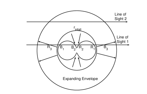
Figure 3: A schematic illustration of the envelope expansion with core collapse (EECC) scenario for generating red profiles of asymmetric molecular line transitions. The cloud consists of an outer expanding envelope and an inner collapsing core, separated by an outgoing spherical surface at $r=r_{\rm infall}$ in a self-similar radial expansion. The loci (i.e. the two connected partial ovals inside the infall radius $r_{\rm infall}$) and two straight arrow lines pointing right of particularly chosen constant projected line-of-sight velocity components are shown as examples. Line of Sight 1 passes through the core of central infall as well as the outer expanding envelope, that intercepts the ovals and straight arrow lines at three points B₁, B₂ and B₃ for the same approaching projected velocity components and at three points R₁, R₂ and R₃ for the same receding projected velocity components. Sufficiently far away from the cloud centre, Line of Sight 2 passes completely through the outer expanding envelope.

Why does our EECC dynamic model lead to the red profiles of molecular spectral lines? Before formal radiative transfer calculations, we would present a schematic analysis in Fig. 3. Line of Sight 1, which is close to the cloud core centre, intercepts the ovals and straight arrow lines at points labelled ‘B’ and ‘R’ for the same approaching and receding projected velocity components, respectively. The intensity of an optically thick transition at a certain frequency will be dominated by emission from the nearest component to the observer, i.e. R₁ and B₃ along Line of Sight 1, because of the absorption and scattering along the path. Assuming the local thermal equilibrium (LTE) for simplification, when the gas temperature increases towards the core centre (as for the case in the bottom panel of Fig. 2), emission from point R₁ will be stronger than that from point B₃, which then gives rise to the asymmetric red profile feature in double-peaked molecular line profiles. On the other hand, as Line of Sight 2 passes completely through the expanding envelope, no ‘red profile’ feature would be detected in this situation.

For a more detailed analysis, we would first invoke the following radiative transfer equation (e.g. Chandrasekhar, 1960; Rybicki & Lightman, 1978), namely

$$\frac{d}{d\tau}I_{\nu}=-I_{\nu}+S_{\nu}\ ,$$ (17)

with $\tau$ being the optical depth, $S$ being the source function and $I$ being the radiative intensity; subscript $\nu$ denotes that these variables are all at a particular frequency $\nu$. Then the radiative intensity at blue and red shifted frequencies are

$$I_{\rm blue}=S_{1}(1-e^{-\tau_{1}})e^{-(\tau_{2}+\tau_{3})}\qquad\qquad\qquad\qquad\qquad$$ (18)

$$\qquad\qquad\qquad+S_{2}(1-e^{-\tau_{2}})e^{-\tau_{3}}+S_{3}(1-e^{-\tau_{3}})\ ,\$$

$$I_{\rm red}=S_{3}(1-e^{-\tau_{3}})e^{-(\tau_{1}+\tau_{2})}\qquad\qquad\qquad\qquad\qquad$$ (19)

$$\qquad\qquad\qquad+S_{2}(1-e^{-\tau_{2}})e^{-\tau_{1}}+S_{1}(1-e^{-\tau_{1}})\ ,$$

respectively, where subscripts 1, 2 and 3 denote variables at three respective positions along Line of Sight 1 shown in Fig. 3. Therefore the difference between the blue-shifted and red-shifted intensities $I_{\rm blue}$ and $I_{\rm red}$ around this frequency is

$$I_{\rm blue}-I_{\rm red}=(S_{3}-S_{1})[1+e^{-(\tau_{1}+\tau_{2}+\tau_{3})}]\qquad\qquad$$ (20)

$$\qquad+(S_{2}-S_{3})[e^{-\tau_{3}}-e^{-(\tau_{1}+\tau_{2})}]\qquad$$

$$\qquad\qquad\qquad\qquad\qquad+(S_{1}-S_{2})[e^{-\tau_{1}}-e^{-(\tau_{2}+\tau_{3})}]\ .$$

Under the LTE condition and the Rayleigh-Jeans approximation for a blackbody source function (e.g. Rybicki & Lightman, 1978), intensities can be expressed in units of brightness temperatures. Therefore the difference between the blue-shifted and red-shifted peak brightness temperatures $T_{\rm blue}$ and $T_{\rm red}$ is

$$T_{\rm blue}-T_{\rm red}=(T_{3}-T_{1})[1+e^{-(\tau_{1}+\tau_{2}+\tau_{3})}]\qquad\qquad$$ (21)

$$\qquad+(T_{2}-T_{3})[e^{-\tau_{3}}-e^{-(\tau_{1}+\tau_{2})}]\qquad$$

$$\qquad\qquad\qquad\qquad\qquad+(T_{1}-T_{2})[e^{-\tau_{1}}-e^{-(\tau_{2}+\tau_{3})}]\ .$$

We can immediately conclude from equation (21) that in an optically thick cloud environment (i.e. $\tau_{1}\gg 1$, $\tau_{2}\gg 1$, $\tau_{3}\gg 1$), the difference in peak brightness temperatures $T_{\rm blue}-T_{\rm red}\approx T_{3}-T_{1}$. Since the gas temperature generally tends to increase towards the cloud centre, i.e. $T_{2}>T_{1}>T_{3}$, we then have $T_{\rm blue}-T_{\rm red}<0$ corresponding to the red-shifted peak intensity being greater than the blue-shifted peak intensity (i.e. an asymmetric red profile). In the opposite limit of optically thin regime (i.e. $\tau_{1}\ll 1$, $\tau_{2}\ll 1$, $\tau_{3}\ll 1$), the difference in brightness temperatures $T_{\rm blue}-T_{\rm red}\approx 0$, indicating that we will get equal peak intensities in blue- and red-shifted frequencies. When the blue- and red-shifted frequencies change (i.e. the loci of equal-projection velocity changes), all foregoing analytical results remain valid. Therefore we can apply these results to the entire blue- and red-shifted peaks in molecular spectral line profiles, and the following conclusion can be reached: double peaked molecular line profiles with stronger red peaks than blue peaks (i.e. red profiles) form under the optical thick condition in a dynamic EECC cloud core. If the outer expanding envelope is replaced by a static envelope, we would then have blue profiles for molecular transitions for optically thick lines along the Line of Sight 1 in Fig. 3 (see also Gao, Lou & Wu 2009 for more details).

4 Data Fitting of EECC Shock Model

4.1 Molecular Spectral Line Profiles

Adopting this EECC shock dynamic solution to model FeSt 1-457, we perform radiative transfer calculations for HCO⁺ (J$=1-0$) line profiles using the RATRAN code (Hogerheijde & van der Tak, 2000) with spherical symmetry. The Doppler b parameter in the code is taken as 0.1 km s^-1, corresponding to an intrinsic line broadening of 0.17 km s^-1. We introduced twelve shells with different thickness (more concentrated towards the cloud central region to account for the rapid variation of physical properties there) in performing the calculations. The dust emissivity follows the model of Ossenkopf & Henning (1994) with bare ice mantles and with $\sim 10^{5}$ years of growth. The abundance ratio of HCO⁺ to H₂ in this cloud core is listed in Table 1. Abundance variations in radius $r$ would affect molecular line profiles (e.g. Tsamis et al., 2008). Here a constant abundance with a central fractional drop (i.e. a step function) appears to be a sensible prescription (see also Evans et al., 2005; Tafalla et al., 2006). Physically, molecular abundance ratios vary with the initial metal compositions and the evolution history of a molecular cloud (e.g. Tsamis et al., 2008); and the central abundance drop is caused by adhesions of molecules onto dust grains in a relatively higher temperature environment (e.g. Tafalla et al., 2006). In the molecular spectral line profile fittings here, abundance values and the radii of abundance holes (see Table 1) in the step function serve as additional fitting parameters to achieve reasonable agreements between our model results and the observational data.

Given the beam width of $\sim 24^{\prime\prime}$, we average our model spectral line profiles over a beam area of $\sim 24^{\prime\prime}\times 24^{\prime\prime}$ and multiply a beam efficiency of $\sim 0.75$ for the IRAM 30m telescope (dotted curves in Fig. 1) to fit the line profile data. Fairly reasonable overall fits of model line profiles to those actually observed ‘red profiles’ (solid curves in Fig. 1 from Aguti et al., 2007) support EECC shock dynamic structures (Fig. 2) for the dark globule FeSt 1-457. Red profiles and red-skewed single peak line profiles in Fig. 1 are encouraging indicators of expansive motions present within this cloud core. In particular, the central $3\times 3$ grids show good agreements between observations and the results of spherical EECC shock model, suggesting that the spherical global expansion is at least a sensible first-order dynamic pattern characterizing the molecular cloud core FeSt 1-457. Certain deviations of spectral line profiles towards the right bottom grids in Fig. 1 then suggest that there might be a beamed outflow or certain rotations [as have been discussed in Gao & Lou (2010)] overlapped with the global envelope expansive motions described by the spherically symmetric model. We may infer from the differences between model results and observations in Fig. 1 that this additional asymmetric motions are of the order of $\sim 0.1{\ \rm km~{}s^{-1}}$.

Table 1: Molecular line transition properties: $\nu_{0}$ is the rest-frame central frequency of the line transition; X₀ is the molecular abundance with respect to H₂ molecules in the cloud core FeSt 1-457; and $r_{\rm h}$ is the radius of the central abundance hole, within which a fractional abundance drop of $10^{-4}$ is presumed.^a

${\rm Molec.}$	${\rm Trans.}$	$\nu_{0}{\rm(GHz)}$	X0	$r_{\rm h}{\rm(cm)}$	Note
HCO+	J$=1-0$	89.19	2$\times 10^{-9}$	7.5 $\times 10^{16}$
HCO+	J$=3-2$	267.56	2$\times 10^{-9}$	7.5 $\times 10^{16}$	b
CS	J$=2-1$	97.98	3$\times 10^{-9}$	1.05$\times 10^{17}$
CS	J$=3-2$	146.97	3$\times 10^{-9}$	1.05$\times 10^{17}$	b
C18O	J$=1-0$	109.78	1$\times 10^{-7}$	6.0 $\times 10^{16}$	c

^a Frequency values are taken from the LAMDA (e.g. Schöier et al., 2005) and abundance values are close to those of Tafalla et al. (2006) with slight variations.
^b Theoretical model predictions for future observational tests.
^c The abundance of C¹⁸O is enhanced to ten times the value of $X_{0}$ for cloud radius $r>1.80\times 10^{17}$ cm.

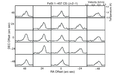
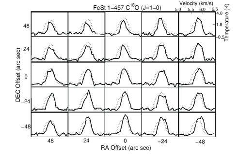
Figure 4: Similar spatially-resolved grid-maps as shown in Fig. 1, but here for CS J$=2-1$ (top panel) and C¹⁸O J$=1-0$ (bottom panel) molecular spectral line transitions. The receding velocity of cloud core FeSt 1-457 along the line of sight is estimated as 5.75 km s^-1. Spectral line fits are done using the same underlying polytropic EECC shock dynamic model described in the text, with step abundance profiles summarized in Table 1.

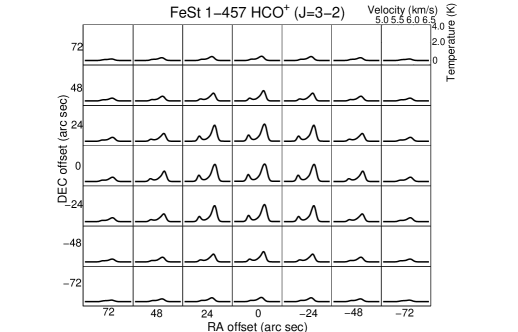
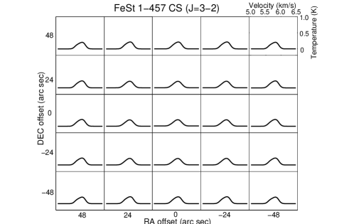
Figure 5: Theoretical model predictions for the molecular transitions HCO⁺ J$=3-2$ (top panel) and CS $J=3-2$ (bottom panel) in spatially-resolved grid-maps of cloud core FeSt 1-457 on the basis of our best-fit EECC hydrodynamic shock model (see Section 3.2 for model details). Each grid has the velocity as the abscissa (with the line-of-sight receding velocity 5.75 km s^-1 of FeSt 1-457) and the antenna temperature (for a 30m IRAM telescope beam efficiency of 0.75) as the ordinate. Model spectral profiles are convolved with a typical beam width of $\sim 24^{\prime\prime}$. The spatially-resolved grid-map is centered at the right ascension $\alpha_{J2000}=17^{\rm h}35^{\rm m}47.5^{\rm s}$ and the declination $\delta_{J2000}=-25^{\circ}33^{\prime}2.0^{\prime\prime}$, with a grid spacing of $24^{\prime\prime}$. The predication of HCO⁺ J$=3-2$ emissions cover a maximum area of $168^{\prime\prime}\times 168^{\prime\prime}$; while for CS $J=3-2$ emissions, the spatial distribution is $120^{\prime\prime}\times 120^{\prime\prime}$. Molecular abundance information are summarized in Table 1.

Meanwhile, spatially-resolved CS (J$=2-1$) and C¹⁸O (J$=1-0$) spectral line profiles are also computed using the RATRAN code given the same underlying EECC shock dynamic model and fitted with observational data of FeSt 1-457 shown in Fig. 4. The CS and C¹⁸O abundance ratios are also prescribed as step functions as listed in Table 1. In running the RATRAN code for radiative transfer calculations, molecular transition data of HCO⁺, CS and C¹⁸O are all taken from the Leiden Atomic and Molecular Database (LAMDA; Schöier et al., 2005). The reasonable fits of CS J$=2-1$ and C¹⁸O J$=1-0$ model molecular line profiles using the same EECC shock dynamic model to the observed corresponding line profiles (see Fig. 4) confirm the viability of the underlying EECC shock model. In comparison with spatially-resolved spectral line profiles of HCO⁺ J$=1-0$, the observed CS J$=2-1$ and C¹⁸O J$=1-0$ spectral line profiles show less asymmetric features because of the relatively lower optical depths in these two molecular line transitions. Both Figs. 1 and 4 show somewhat notable deviations between model spectral line profiles and those observed at grids in the lower right of the map, which is most likely associated with non-spherical symmetry of any realistic astrophysical systems. We may infer from these complementary molecular line model fittings, though with less asymmetries in line profiles, that the spherically symmetric EECC model represents a reasonable description to this particular star-forming cloud. It is expected that more structural complexities on smaller scales (e.g. Redman et al. 2004 for rotations and Carolan et al. 2008 for bipolar outflows etc.) can complicate such radiative transfer fittings.

As testable theoretical predictions for future telescope observations of the HCO⁺ J$=3-2$ and CS J$=3-2$ emission lines from the cloud core FeSt 1-457, we show our model calculation results as predictions in Fig. 5. Besides that all these predictions are based on the same EECC hydrodynamic shock model described in Section 3.2, abundance profiles of HCO⁺ and CS remain also the same as what we have used to calculate HCO⁺ J$=1-0$ and CS J$=2-1$ molecular line transitions (see Table 1). Molecular transitions HCO⁺ J$=3-2$ and CS J$=3-2$ emissions have higher excitation temperatures than those for HCO⁺ J$=1-0$ and CS J$=2-1$ emissions, respectively (e.g. Schöier et al., 2005). Therefore in the environment temperature of only $\sim 10$ K in a cloud, they are less excited and thus have lower emission intensities as shown in Fig. 5. The intensities of CS J$=3-2$ emissions are even weaker because of a larger central abundance hole presumed (see Table 1). Because the abundance hole is large, less higher temperature cloud regions will contribute to the line emission, which makes the CS J$=3-2$ emission very weak. This leads the conclusion that for certain molecules, the radius of the abundance hole will affect the intensity contrast between its transition lines with higher and lower excitation temperatures. We may also learn from Fig. 1 and Fig. 5 that optically thin molecular transition lines (here HCO⁺ J$=3-2$) show less asymmetries in line profiles than optically thick transition lines (here HCO⁺ J$=1-0$). That is why optically thick lines are more sensitive diagnostics of hydrodynamic structures in molecular clouds.

4.2 Column Density and Dust Continuum Profiles

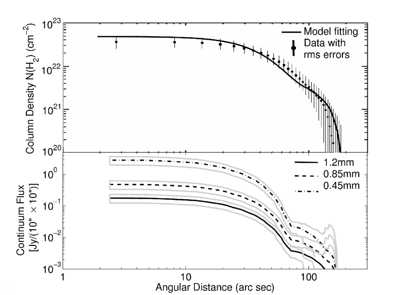
Figure 6: Radial profiles of column number density (top panel) and predicted (sub)millimetre continuum emissions (bottom panel) are shown here. The top panel compares the radial profile of column number density derived from the EECC hydrodynamic shock model (solid curve) and the data with error bars inferred from dust extinction observations (Kandori et al., 2005, dots with errors). Error bars are root-mean-square (RMS) scatters of data points within each annulus. The radial profile derived from the EECC hydrodynamic shock model is convolved with the observational spatial resolution of $\sim 30^{\prime\prime}$. The same EECC hydrodynamic shock model that fits molecular spectral line profiles in Fig. 1 also offers a fair fitting (within RMS errors) to the radial profile of column density. The bottom panel shows continuum emission intensities at three wavelengths of 1.2 mm, 0.85 mm and 0.45 mm, which are predicted here for future observational tests. These (sub)millimetre continuum profiles are derived using the same underlying EECC shock dynamic model, with dust opacities given by Ossenkopf & Henning (1994) in the case of bare ice mantles and $\sim 10^{5}$ yr growth, and convolved with a typical spatial resolution of $\sim 10^{\prime\prime}\times 10^{\prime\prime}$. Three pairs of gray curves along the three predicted continuum profiles show relevant ranges of uncertainties in the (sub)millimetre continuum emissions, which are estimated according to RMS errors in the column number density observation, using the relationship $I_{\nu}\propto\rho^{1.2}$. Abrupt turns around $\sim 70^{\prime\prime}$ signal shock discontinuities and might be detected with high enough spatial resolutions.

The dust extinction observation of FeSt 1-457 of Kandori et al. (2005) represents an important observational constraint to the model description of this molecular cloud core. We infer from Fig. 2 of Kandori et al. (2005) that the cloud core FeSt 1-457 appears grossly spherical, yet with slight asymmetry towards the lower right corner. This asymmetry in the dust extinction observation coincides with the differences shown in spectral line profile model fittings as shown in Figs. 1 and 4. All these available observations might imply that there exists some kind of beamed outflows towards the lower right direction in FeSt 1-457, in addition to an almost spherically symmetric cloud core. As the deviation of molecular lines in this part of the cloud core is toward red-shifted in the order of $\sim 0.1\ {\rm km~{}s^{-1}}$ (see Figs. 1 and 4), we estimate that a beamed slow outflow may recede from us with a typical speed of $\sim 0.1\ {\rm km~{}s^{-1}}$.

As a further consistent model check, we compute the radial profile of column density using the same EECC shock dynamic model and compare it with that inferred from the dust extinction data for FeSt 1-457 (Kandori et al., 2005). As the column density data has a spatial resolution of $30^{\prime\prime}$, our computed model profile is derived from the same EECC shock dynamic model with a convolution in $30^{\prime\prime}$ and shows a sensibly good fit (the top panel of Fig. 6). As the radial profile of column density is sensitive to the outer radius $R_{\rm out}$ of the molecular cloud core and to the cloud number density $N$, this fit identifies a proper outer radius $R_{\rm out}$ and the molecular hydrogen H₂ number density scale (see eqn (16)). The outer radius of FeSt 1-457 used in the column density fit is $R_{\rm out}=1.8\times 10^{4}$ au, which is also used in molecular spectral line profile fits and appears consistent with that from the optical images (Aguti et al., 2007) at the same time. In short, the inferred variation trend of column density offers a constraint on a proper EECC shock dynamic phase with a grossly self-consistent radial density profile.

In previous publications (e.g. Alves, Lada & Lada, 2001; Harvey et al., 2003; Kandori et al., 2005) regarding the column density structure of molecular clouds, researchers normally use a power-law radial density distribution or a static Bonnor-Ebert sphere (Bonnor, 1956; Ebert, 1955) etc. to describe density distributions within observed molecular clouds. These empirical/theoretical models also appear to provide reasonable fits to the observationally inferred radial column density distributions, but none of them have been shown to successfully account for the observed molecular spectral line profiles from those molecular clouds, except that additional parameterized conditions are introduced (e.g. Tafalla et al., 2006). In contrast, our theoretical cloud models involving proper hydrodynamic flows and with self-consistent radial temperature variations can give rise to asymmetric molecular line profiles (Gao, Lou & Wu, 2009; Gao & Lou, 2010). According to the Bonnor-Ebert sphere model fits to a group of cloud cores in Kandori et al. (2005), most of those best-fit static spheres are actually unstable Bonnor-Ebert spheres, implying that these molecular cloud cores are most likely undergoing hydrodynamic evolution in reality. Another data analysis by Li et al. (2007) on massive quiescent cores in the Orion molecular cloud, gives a similar result that most of the cloud cores are unstable, if modelled as static Bonnor-Ebert spheres. All these results hint that we do need a theoretical model formulation for the hydrodynamic evolution of cloud cores. That is, the spectral line profiles and dust emission data fitting are not inconsistent with our EECC dynamic shock model. Essentially similar problems also exist in the model fits of dust continuum emission observations described immediately below. Therefore to be consistently constrained by all available observations, we explore the polytropic EECC hydrodynamic shock model here for the molecular cloud core FeSt 1-457.

Radial profiles of (sub)millimetre continua at three wavelengths can be also computed using the RATRAN code to further check the consistency for the density and temperature radial structures of cloud cores. For these testable observations (e.g. Shirley et al., 2000, 2002, for other cloud systems), we specifically predict such continuum radial profiles at three wavelengths of 1.2 mm, 0.85 mm and 0.45 mm using the same underlying EECC hydrodynamic shock model for FeSt 1-457. Modelling such dust continuum emissions as optically thin with a constant dust opacity $\kappa_{\nu}$ in $r$ at a specified frequency $\nu$, the observed intensity at an impact parameter $b$ is (Adams, 1991; Shirley et al., 2002) given by

$$I_{\nu}(b)=2\int_{b}^{R_{\rm out}}B_{\nu}(T_{\rm d})\frac{\kappa_{\nu}\rho(r)r}{(r^{2}-b^{2})^{1/2}}dr\ ,$$ (22)

where $T_{\rm d}(r)$ is the dust temperature taken to be the same as the H₂ gas temperature $T(r)$, $\rho(r)$ is the mass density of H₂ molecules and $B_{\nu}(T_{\rm d})$ is the Planck function. The opacity $\kappa_{\nu}$ is that of Ossenkopf & Henning (1994) dust model for bare ice mantles with a growth time of $\sim 10^{5}$ yr. As usual, a H₂ gas to dust mass ratio 100 to 1 is adopted in our model computations. With the dust temperature and density profiles from the EECC hydrodynamic shock model, we obtain radial profiles for 1.2 mm, 0.85 mm and 0.45mm continuum intensities. Results shown in the bottom panel of Fig. 6 are convolved with a telescope beam size of $\sim 10^{\prime\prime}\times 10^{\prime\prime}$ and a beam efficiency of $\sim 1$. Error ranges of millimetre continuum intensities are estimated by the root-mean-square (RMS) errors in the column density observation (the upper panel of Fig. 6), through the relation $I_{\nu}\propto\rho^{1.2}$. The abrupt ‘kink’ at $\sim 70^{\prime\prime}$ from the centre reveals shock discontinuities of density and temperature in the EECC shock model (see the middle and bottom panels in Fig. 2), and should be detectable with high enough spatial resolutions.

5 Conclusion and Speculations

We have presented model results pertinent to three complementary observational aspects towards the dark molecular globule FeSt 1-457; fairly reasonable fittings to asymmetric ‘red profiles’ and to the column density radial profile derived from dust extinction data indicate that this dark globule most likely involve an early EECC shock phase of dynamic cloud evolution, while our predictions for spatially-resolved grid-maps for HCO⁺ J$=3-2$ and CS J$=3-2$ respectively as well as the three predicted millimetre continuum radial profiles can be specifically tested by future observations. The choice of our model parameter set is determined by an extensive exploration and known quantitative as well as qualitative constraints. Slight adjustment around this chosen model parameter set is allowed for a refined improvement of fitting. Although without a rigorous proof, it would be surprising that a dramatically different model parameter set could reproduce all the available observational data so far. In addition to the spherical global EECC dynamics, line profile and extinction observations might also suggest a slow beamed outflow receding from us at a typical speed of $\sim 0.1{\ \rm km~{}s^{-1}}$ towards the lower right direction in the grid-maps. The inferred underlying EECC hydrodynamic shock model provides physical parameters for FeSt 1-457 cloud core. The central protostellar mass blob and the total mass of the cloud core are $M_{0}\sim 0.020M_{\odot}$ and $M_{\rm tot}\sim 2.93M_{\odot}$, respectively; the central protostellar mass accretion rate is $\dot{M}_{0}\sim 0.69\times 10^{-7}M_{\odot}~{}{\rm yr^{-1}}$ (see eq (9)); the dynamical timescale of the cloud core FeSt 1-457 is estimated as $t\sim 2.8\times 10^{5}~{}{\rm yr}$ accordingly (see expression (16)). As an expanding shock travels through the molecular cloud core, abundance differences of certain tracer molecules (e.g. CH₃OH and SiO) across the shock front (e.g. Jørgensen et al., 2004) could be detectable.

As a strong supporting evidence to the present case of FeSt 1-457, a parallel theoretical model analysis on another star-forming molecular cloud core L1517B has also been conducted and completed recently (Fu, Gao & Lou, 2010). Several molecular line transitions of L1517B also manifest red asymmetric line profiles. On the basis of a shocked EECC similarity hydrodynamic model, several single point central molecular emission lines of HCO⁺($1-0$), HCO⁺($3-2$), H¹³CO⁺($1-0$), DCO⁺($3-2$), H₂CO($2_{12}-1_{11}$), H₂CO($2_{11}-1_{10}$), CS($2-1$), CS($3-2$), SO($23-12$), and SO($34-23$) from the source L1517B [observed by 13.7 m telescope of the Five College Radio Astronomical Observatory (FCRAO) and IRAM 30 m telescope] are simultaneously fitted in an overall consistent manner. Taking into account of the fact that spatially-resolved HCO⁺ (J$=1-0$) emission line profiles [observed by Delingha 13.7m telescope of the Purple Mountain Observatory (PMO)], as well as 1.2 mm and 850 $\mu$m continuum emissions (observed by IRAM 30 m and JCMT respectively) can be consistently fitted by the same underlying EECC hydrodynamic shock model, we are fairly confident that the cloud core L1517B appears to be another cloud core that evolves in the EECC shock phase. Similar to what we have done for FeSt 1-457 here, predictions of several other spatially-resolved molecular transition lines, the radial profile of 450 $\mu$m continuum emission, and visual extinction (all based on the same EECC hydrodynamic shock model) are also presented for further observational tests of the model description of L1517B (see Fu, Gao & Lou (2010) for details).

We speculate that other starless cores of grossly spherical molecular clouds with ‘red profiles’ might also involve EECC hydrodynamic shock phase in general. More sources need to be search and established by systematic model analysis and data comparisons. The existence of global EECC hydrodynamic shock at early phases would affect the formation of protostars and their surroundings, including estimates for star formation rates and initial mass functions that need to be further explored.

References

- Adams (1991) Adams F. C., 1991, ApJ, 382, 544
- Aguti et al. (2007) Aguti E. D., Lada C. J., Bergin E. A., Alves J. F., Birkinshaw M., 2007, ApJ, 665, 457
- Alves, Lada & Lada (2001) Alves J. F., Lada C. J., Lada E. A., 2001, Nature, 409, 159
- Bian & Lou (2005) Bian F.-Y., Lou Y.-Q., 2005, MNRAS, 363, 1315
- Bonnor (1956) Bonnor W., 1956, MNRAS, 116, 351
- Chandrasekhar (1960) Chandrasekhar S., 1960 Radiative Transfer, Dover Press, New York
- Carolan et al. (2008) Carolan P. B., Redman M. P., Keto E., Rawlings J. M. C., 2008, MNRAS, 383, 705
- Di Francesco et al. (2001) Di Francesco J., Myers P. C., Wilner D. J., Ohashi N., Mardones D., 2001, ApJ, 562, 770
- Ebert (1955) Ebert R., 1955, Z. f Astr., 37, 217
- Evans (2003) Evans N. J. II, 2003, in Proc. of Conf., Chemistry as a Diagnostic of Star Formation, eds. Curry C. L., Fich M., NRC Research Press, Ottawa, Canada, p.157
- Evans et al. (2005) Evans N. J. II, Lee J.-E., Rawlings J. M. C., Choi M. 2005, ApJ, 626, 919
- Fiege & Henriksen (1996) Fiege J. D., Henriksen R. N., 1996, MNRAS, 281, 1055
- Fu, Gao & Lou (2010) Fu T. M., Gao Y., Lou Y.-Q., 2010, submitted
- Gao, Lou & Wu (2009) Gao Y., Lou Y.-Q., Wu K., 2009, MNRAS, 400, 878
- Gao & Lou (2010) Gao Y., Lou Y.-Q., 2010, MNRAS, 403, 1919
- Greve, Kramer & Wild (1998) Greve A., Kramer C., Wild W., 1998, A&A Suppl., 133, 271
- Harvey et al. (2003) Harvey D. W. A., Wilner D. J., Lada C. J., Myers P. C., 2003, ApJ, 598, 1112
- Hogerheijde & van der Tak (2000) Hogerheijde M. R., van der Tak, F. F. S., 2000, A&A, 362, 697
- Jørgensen et al. (2004) Jørgensen J. K., Hogerheijde M. R., Blake G. A., van Dishoeck E. F., Mundy L. G., Schöier F. L., 2004, A&A, 415, 1021
- Kandori et al. (2005) Kandori R. et al., 2005, AJ, 130, 2166
- Lada et al. (2003) Lada C. J., Bergin E. A., Alves J. F., Huard T. L., 2003, ApJ, 586, 286
- Li et al. (2007) Li D., Velusamy T., Goldsmith P. F., Langer W. D., 2007, ApJ, 655, 351
- Lombardi, Alves & Lada (2006) Lombardi M., Alves J., Lada C. J., 2006, A&A, 454, 781
- Lou & Shen (2004) Lou Y.-Q., Shen Y., 2004, MNRAS, 348, 717
- Lou & Gao (2006) Lou Y.-Q., Gao Y., 2006, MNRAS, 373, 1610
- Mardones et al. (1997) Mardones D., Myers P. C., Tafalla M., Wilner D. J., 1997, ApJ, 489, 719
- McKee & Tan (2002) McKee C. F., Tan J. C., 2002, Nature, 416, 59
- McLaughlin & Pudritz (1997) McLaughlin D. E., Pudritz R. E., 1997, ApJ, 476, 750
- Motte & André (2001) Motte F., André P., 2001, A&A, 365, 440
- Ossenkopf & Henning (1994) Ossenkopf V., Henning T., 1994, A&A, 291, 943
- Ossenkopf (2002) Ossenkopf V., 2002, A&A, 391, 295
- Rawlings & Yates (2001) Rawlings J. M. C., Yates J. A., 2001, MNRAS, 326, 1423
- Redman et al. (2004) Redman M. P., Keto E., Rawlings J. M. C., Williams D. A., 2004, MNRAS, 352, 1365
- Rybicki & Lightman (1978) Rybicki G. B., Lightman A., 1978, Radiative Processes in Astrophysics, 2nd ed., John Wiley & Sons, New York
- Schöier et al. (2005) Schöier F. L., van der Tak F. F. S., van Dishoeck E. F., Black J. H., 2005, A&A 432, 369
- Shen & Lou (2004) Shen Y., Lou Y.-Q., 2004, ApJ, 611, L117
- Shen & Lou (2006) Shen Y., Lou Y.-Q., 2006, MNRAS, 370, L85
- Shirley et al. (2000) Shirley Y. L., Evans N. J. E., Rawlings J. M. C., Gregersen E. M., 2000, ApJS, 131, 249
- Shirley et al. (2002) Shirley Y. L., Evans N. J. E., Rawlings J. M. C., 2002, ApJ, 575, 337
- Shu (1977) Shu F. H., 1977, ApJ, 214, 488
- Shu, Adams & Lizano (1987) Shu F. H., Adams F. C., Lizano S., 1987, ARA&A, 25, 23
- Tafalla et al. (2000) Tafalla M., Mardones D., Myers P. C., Bachiller R., 2000, A&A, 359, 967
- Tafalla et al. (2006) Tafalla M., Santiago J., Myers P. C., Caselli P., Walmsley C. M., Crapsi A., 2006, A&A, 455, 577
- Thompson & White (2004) Thompson M. A., White G. J., 2004, A&A, 419, 599
- Tsamis et al. (2008) Tsamis Y. G., Rawlings J. M. C., Yates J. A., Viti S., 2008, MNRAS, 388, 898
- Velusamy et al. (2008) Velusamy T., Peng R., Li D., Goldsmith P. F., Langer W. D., 2008, ApJ, 688, L87
- Wang & Lou (2007) Wang W.-G., Lou Y.-Q., 2007, Ap&SS, 311, 363
- Wang & Lou (2008) Wang W.-G., Lou Y.-Q., 2008, Ap&SS, 315, 135
- Zhou et al. (1993) Zhou S., Evans N. J. II, Kömpe C., Walmsley C. M., 1993, ApJ, 404, 232