Strong Rules for Discarding Predictors in Lasso-type Problems

Abstract

We consider rules for discarding predictors in lasso regression and related problems, for computational efficiency. safe propose “SAFE” rules, based on univariate inner products between each predictor and the outcome, that guarantee a coefficient will be zero in the solution vector. This provides a reduction in the number of variables that need to be entered into the optimization. In this paper, we propose strong rules that are not foolproof but rarely fail in practice. These are very simple, and can be complemented with simple checks of the Karush-Kuhn-Tucker (KKT) conditions to ensure that the exact solution to the convex problem is delivered. These rules offer a substantial savings in both computational time and memory, for a variety of statistical optimization problems.

1 Introduction

Our focus here is on statistical models fit using $\ell_{1}$ regularization. We start with penalized linear regression. Consider a problem with $N$ observations and $p$ predictors, and let $\mathbf{y}$ denote the $N$-vector of outcomes, and $\mathbf{X}$ be the $N\times p$ matrix of predictors, with $j$th column $\mathbf{x}_{j}$ and $i$th row $x_{i}$. For a set of indices $\mathcal{A}=\{j_{1},\ldots j_{k}\}$, we write $\mathbf{X}_{\mathcal{A}}$ to denote the $N\times k$ submatrix $\mathbf{X}_{\mathcal{A}}=[\mathbf{x}_{j_{1}},\ldots\mathbf{x}_{j_{k}}]$, and also $\mathbf{b}_{\mathcal{A}}=(b_{j_{1}},\ldots b_{j_{k}})$ for a vector $\mathbf{b}$. We assume that the predictors and outcome are centered, so we can omit an intercept term from the model.

The lasso lasso solves the optimization problem

$$\hat{{\bm{\beta}}}=\mathop{\mathrm{argmin}}_{{\bm{\beta}}}\;\frac{1}{2}\|\mathbf{y}-\mathbf{X}{\bm{\beta}}\|_{2}^{2}+\lambda\|{\bm{\beta}}\|_{1},$$ (1)

where $\lambda\geq 0$ is a tuning parameter. There has been considerable work in the past few years deriving fast algorithms for this problem, especially for large values of $N$ and $p$. A main reason for using the lasso is that the $\ell_{1}$ penalty tends to give exact zeros in $\hat{{\bm{\beta}}}$, and therefore it performs a kind of variable selection. Now suppose we knew, a priori to solving (1), that a subset of the variables $S\subseteq\{1,\ldots p\}$ will have zero coefficients in the solution, that is, $\hat{{\bm{\beta}}}_{S}=0$. Then we could solve problem (1) with the design matrix replaced by $\mathbf{X}_{S^{c}}$, where $S^{c}=\{1,\ldots p\}\setminus S$, for the remaining coefficients $\hat{{\bm{\beta}}}_{S^{c}}$. If $S$ is relatively large, then this could result in a substantial computational savings.

safe construct such a set $S$ of “screened” or “discarded” variables by looking at the inner products $|\mathbf{x}_{j}^{T}\mathbf{y}|$, $j=1,\ldots p$. The authors use a clever argument to derive a surprising set of rules called “SAFE”, and show that applying these rules can reduce both time and memory in the overall computation. In a related work, Wu2009 study $\ell_{1}$ penalized logistic regression and build a screened set $S$ based on similar inner products. However, their construction does not guarantee that the variables in $S$ actually have zero coefficients in the solution, and so after fitting on $\mathbf{X}_{S^{c}}$, the authors check the Karush-Kuhn-Tucker (KKT) optimality conditions for violations. In the case of violations, they weaken their set $S$, and repeat this process. Also, FL2008 study the screening of variables based on their inner products in the lasso and related problems, but not from a optimization point of view. Their screening rules may again set coefficients to zero that are nonzero in the solution, however, the authors argue that under certain situations this can lead to better performance in terms of estimation risk.

In this paper, we propose strong rules for discarding predictors in the lasso and other problems that involve lasso-type penalties. These rules discard many more variables than the SAFE rules, but are not foolproof, because they can sometimes exclude variables from the model that have nonzero coefficients in the solution. Therefore we rely on KKT conditions to ensure that we are indeed computing the correct coefficients in the end. Our method is most effective for solving problems over a grid of $\lambda$ values, because we can apply our strong rules sequentially down the path, which results in a considerable reduction in computational time. Generally speaking, the power of the proposed rules stems from the fact that:

• the set of discarded variables $S$ tends to be large and violations rarely occur in practice, and

• the rules are very simple and can be applied to many different problems, including the elastic net, lasso penalized logistic regression, and the graphical lasso.

In fact, the violations of the proposed rules are so rare, that for a while a group of us were trying to establish that they were foolproof. At the same time, others in our group were looking for counter-examples [hence the large number of co-authors!]. After many flawed proofs, we finally found some counter-examples to the strong sequential bound (although not to the basic global bound). Despite this, the strong sequential bound turns out to be extremely useful in practice.

Here is the layout of this paper. In Section 2 we review the SAFE rules of safe for the lasso. The strong rules are introduced and illustrated in Section 3 for this same problem. We demonstrate that the strong rules rarely make mistakes in practice, especially when $p\gg N$. In Section 4 we give a condition under which the strong rules do not erroneously discard predictors (and hence the KKT conditions do not need to be checked). We discuss the elastic net and penalized logistic regression in Sections 5 and 6. Strong rules for more general convex optimization problems are given in Section 7, and these are applied to the graphical lasso. In Section 8 we discuss how the strong sequential rule can be used to speed up the solution of convex optimization problems, while still delivering the exact answer. We also cover implementation details of the strong sequential rule in our glmnet algorithm (coordinate descent for lasso penalized generalized linear models). Section 9 contains some final discussion.

2 Review of the SAFE rules

The basic SAFE rule of safe for the lasso is defined as follows: fitting at $\lambda$, we discard predictor $j$ if

$$|\mathbf{x}_{j}^{T}\mathbf{y}|<\lambda-\|\mathbf{x}_{j}\|_{2}\|\mathbf{y}\|_{2}\frac{\lambda_{\mathrm{max}}-\lambda}{\lambda_{\mathrm{max}}},$$ (2)

where $\lambda_{\mathrm{max}}=\max_{i}|\mathbf{x}_{i}^{T}\mathbf{y}|$ is the smallest $\lambda$ for which all coefficients are zero. The authors derive this bound by looking at a dual of the lasso problem (1). This is:

$$\hat{{\bm{\theta}}}= \mathop{\mathrm{argmax}}_{\bm{\theta}}\;G({\bm{\theta}})=\frac{1}{2}\|\mathbf{y}\|_{2}^{2}-\frac{1}{2}\|\mathbf{y}+{\bm{\theta}}\|_{2}^{2}$$ (3)

$$\text{subject to}\;\;|\mathbf{x}_{j}^{T}{\bm{\theta}}|\leq\lambda\;\;\text{for}\;j=1,\ldots p.$$

The relationship between the primal and dual solutions is $\hat{{\bm{\theta}}}=\mathbf{X}\hat{{\bm{\beta}}}-\mathbf{y}$, and

$$\mathbf{x}_{j}^{T}\hat{{\bm{\theta}}}\in\begin{cases}\{+\lambda\}&\text{if}\;\;\hat{\beta}_{j}>0\\ \{-\lambda\}&\text{if}\;\;\hat{\beta}_{j}<0\\ [-\lambda,\lambda]&\text{if}\;\;\hat{\beta}_{j}=0\end{cases}$$ (4)

for each $j=1,\ldots p$. Here is a sketch of the argument: first we find a dual feasible point of the form ${\bm{\theta}}_{0}=s\mathbf{y}$, ($s$ is a scalar), and hence $\gamma=G(s\mathbf{y})$ represents a lower bound for the value of $G$ at the solution. Therefore we can add the constraint $G({\bm{\theta}})\geq\gamma$ to the dual problem (3) and nothing will be changed. For each predictor $j$, we then find

$$m_{j}=\mathop{\mathrm{argmax}}_{{\bm{\theta}}}\;|\mathbf{x}_{j}^{T}{\bm{\theta}}|\;\;\text{subject to}\;G({\bm{\theta}})\geq\gamma.$$

If $m_{j}<\lambda$ (note the strict inequality), then certainly at the solution $|\mathbf{x}_{j}^{T}\hat{{\bm{\theta}}}|<\lambda$, which implies that $\hat{\beta}_{j}=0$ by (4). Finally, noting that $s=\lambda/\lambda_{\mathrm{max}}$ produces a dual feasible point and rewriting the condition $m_{j}<\lambda$ gives the rule (2).

In addition to the basic SAFE bound, the authors also derive a more complicated but somewhat better bound that they call “recursive SAFE” (RECSAFE). As we will show, the SAFE rules have the advantage that they will never discard a predictor when its coefficient is truly nonzero. However, they discard far fewer predictors than the strong sequential rule, introduced in the next section.

3 Strong screening rules

3.1 Basic and strong sequential rules

Our basic (or global) strong rule for the lasso problem (1) discards predictor $j$ if

$$|\mathbf{x}_{j}^{T}\mathbf{y}|<2\lambda-\lambda_{\mathrm{max}},$$ (5)

where as before $\lambda_{\mathrm{max}}=\max_{j}|\mathbf{x}_{j}^{T}\mathbf{y}|$.

When the predictors are standardized ($\|\mathbf{x}_{j}\|_{2}=1$ for each $j$), it is not difficult to see that the right hand side of (2) is always smaller than the right hand side of (5), so that in this case the SAFE rule is always weaker than the basic strong rule. This follows since $\lambda_{\mathrm{max}}\leq\|\mathbf{y}\|_{2}$, so that

$$\lambda-\|\mathbf{y}\|_{2}\frac{\lambda_{\mathrm{max}}-\lambda}{\lambda_{\mathrm{max}}}\;\leq\;\lambda-(\lambda_{\mathrm{max}}-\lambda)\;=\;2\lambda-\lambda_{\mathrm{max}}.$$

Figure 1 illustrates the SAFE and basic strong rules in an example.

\psfrag{lm}{$\lambda_{max}$}\psfrag{la}{$\lambda$}\psfrag{lambda}{$\lambda$}\includegraphics[width=216.81pt]{dual.ps}

Figure 1: SAFE and basic strong bounds in an example with 10 predictors, labelled at the right. The plot shows the inner product of each predictor with the current residual, with the predictors in the model having maximal inner product equal to $\pm\lambda$. The dotted vertical line is drawn at $\lambda_{max}$; the broken vertical line is drawn at $\lambda$. The strong rule keeps only predictor #3, while the SAFE bound keeps predictors #8 and #1 as well.

When the predictors are not standardized, the ordering between the two bounds is not as clear, but the strong rule still tends to discard more variables in practice unless the predictors have wildly different marginal variances.

While (5) is somewhat useful, its sequential version is much more powerful. Suppose that we have already computed the solution $\hat{{\bm{\beta}}}(\lambda_{0})$ at $\lambda_{0}$, and wish to discard predictors for a fit at $\lambda<\lambda_{0}$. Defining the residual $\mathbf{r}=\mathbf{y}-\mathbf{X}\hat{{\bm{\beta}}}(\lambda_{0})$, our strong sequential rule discards predictor $j$ if

$$|\mathbf{x}_{j}^{T}\mathbf{r}|<2\lambda-\lambda_{0}.$$ (6)

Before giving a detailed motivation for these rules, we first demonstrate their utility. Figure 2 shows some examples of the applications of the SAFE and strong rules. There are four scenarios with various values of $N$ and $p$; in the first three panels, the $\mathbf{X}$ matrix is dense, while it is sparse in the bottom right panel. The population correlation among the feature is zero, positive, negative and zero in the four panels. Finally, 25% of the coefficients are non-zero, with a standard Gaussian distribution. In the plots, we are fitting along a path of decreasing $\lambda$ values and the plots show the number of predictors left after screening at each stage. We see that the SAFE and RECSAFE rules only exclude predictors near the beginning of the path. The strong rules are more effective: remarkably, the strong sequential rule discarded almost all of the predictors that have coefficients of zero. There were no violations of any of rules in any of the four scenarios.

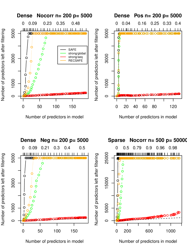
Figure 2: Lasso regression: results of different rules applied to four different scenarios. There are four scenarios with various values of $N$ and $p$; in the first three panels the $\mathbf{X}$ matrix is dense, while it is sparse in the bottom right panel. The population correlation among the feature is zero, positive, negative and zero in the four panels. Finally, 25% of the coefficients are non-zero, with a standard Gaussian distribution. In the plots, we are fitting along a path of decreasing $\lambda$ values and the plots show the number of predictors left after screening at each stage. A broken line with unit slope is added for reference. The proportion of variance explained by the model is shown along the top of the plot. There were no violations of any of the rules in any of the four scenarios.

It is common practice to standardize the predictors before applying the lasso, so that the penalty term makes sense. This is what was done in the examples of Figure 2. But in some instances, one might not want to standardize the predictors, and so in Figure 3 we investigate the performance of the rules in this case. In the left panel the population variance of each predictor is the same; in the right panel it varies by a factor of 50. We see that in the latter case the SAFE rules outperform the basic strong rule, but the sequential strong rule is still the clear winner. There were no violations in any of rules in either panel.

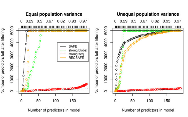
Figure 3: Lasso regression: results of different rules when the predictors are not standardized. The scenario in the left panel is the same as in the top left panel of Figure 2, except that the features are not standardized before fitting the lasso. In the data generation for the right panel, each feature is scaled by a random factor between 1 and 50, and again, no standardization is done.

3.2 Motivation for the strong rules

We now give some motivation for the strong rule (5) and later, the sequential rule (6). We start with the KKT conditions for the lasso problem (1). These are

$$\mathbf{x}_{j}^{T}(\mathbf{y}-\mathbf{X}\hat{{\bm{\beta}}})=\lambda\cdot s_{j}$$ (7)

for $j=1,\ldots p$, where $s_{j}$ is a subgradient of $\hat{\beta}_{j}$:

$$s_{j}\in\begin{cases}\{+1\}&\text{if}\;\;\hat{\beta}_{j}>0\\ \{-1\}&\text{if}\;\;\hat{\beta}_{j}<0\\ [-1,1]&\text{if}\;\;\hat{\beta}_{j}=0.\end{cases}$$ (8)

Let $c_{j}(\lambda)=\mathbf{x}_{j}^{T}\{\mathbf{y}-\mathbf{X}\hat{{\bm{\beta}}}(\lambda)\}$, where we emphasize the dependence on $\lambda$. Suppose in general that we could assume

$$|c_{j}^{\prime}(\lambda)|\leq 1,$$ (9)

where $c_{j}^{\prime}$ is the derivative with respect to $\lambda$, and we ignore possible points of non-differentiability. This would allow us to conclude that

$$|c_{j}(\lambda_{\mathrm{max}})-c_{j}(\lambda)| =\left|\int_{\lambda}^{\lambda_{\mathrm{max}}}c_{j}^{\prime}(\lambda)\,d\lambda\right|$$ (10)

$$\leq\int_{\lambda}^{\lambda_{\mathrm{max}}}|c_{j}^{\prime}(\lambda)|\,d\lambda$$ (11)

$$\leq\lambda_{\mathrm{max}}-\lambda,$$

and so

$$|c_{j}(\lambda_{\mathrm{max}})|<2\lambda-\lambda_{\mathrm{max}}\;\Rightarrow\;|c_{j}(\lambda)|<\lambda\;\Rightarrow\;\hat{\beta}_{j}(\lambda)=0,$$

the last implication following from the KKT conditions, (7) and (8). Then the strong rule (5) follows as $\hat{{\bm{\beta}}}(\lambda_{\mathrm{max}})=0$, so that $|c_{j}(\lambda_{\mathrm{max}})|=|\mathbf{x}_{j}^{T}\mathbf{y}|$.

Where does the slope condition (9) come from? The product rule applied to (7) gives

$$c_{j}^{\prime}(\lambda)=s_{j}(\lambda)+\lambda\cdot s_{j}^{\prime}(\lambda),$$ (12)

and as $|s_{j}(\lambda)|\leq 1$, condition (9) can be obtained if we simply drop the second term above. For an active variable, that is $\hat{\beta}_{j}(\lambda)\not=0$, we have $s_{j}(\lambda)=\mathrm{sign}\{\hat{\beta}_{j}(\lambda)\}$, and continuity of $\hat{\beta}_{j}(\lambda)$ with respect to $\lambda$ implies $s_{j}^{\prime}(\lambda)=0$. But $s_{j}^{\prime}(\lambda)\not=0$ for inactive variables, and hence the bound (9) can fail, which makes the strong rule (5) imperfect. It is from this point of view—writing out the KKT conditions, taking a derivative with respect to $\lambda$, and dropping a term—that we derive strong rules for $\ell_{1}$ penalized logistic regression and more general problems.

In the lasso case, condition (9) has a more concrete interpretation. From lars, we know that each coordinate of the solution $\hat{\beta}_{j}(\lambda)$ is a piecewise linear function of $\lambda$, hence so is each inner product $c_{j}(\lambda)$. Therefore $c_{j}(\lambda)$ is differentiable at any $\lambda$ that is not a kink, the points at which variables enter or leave the model. In between kinks, condition (9) is really just a bound on the slope of $c_{j}(\lambda)$. The idea is that if we assume the absolute slope of $c_{j}(\lambda)$ is at most 1, then we can bound the amount that $c_{j}(\lambda)$ changes as we move from $\lambda_{\mathrm{max}}$ to a value $\lambda$. Hence if the initial inner product $c_{j}(\lambda_{\mathrm{max}})$ starts too far from the maximal achieved inner product, then it cannot “catch up” in time. An illustration is given in Figure 4.

\psfrag{l}{$\lambda$}\psfrag{cjxxxxxxxxxx}{$c_{j}=\mathbf{x}_{j}^{T}(\mathbf{y}-\mathbf{X}\hat{{\bm{\beta}}})$}\psfrag{l0-l1}{$\lambda_{\mathrm{max}}-\lambda_{1}$}\psfrag{l1}{$\lambda_{1}$}\psfrag{l0}{$\lambda_{\mathrm{max}}$}\includegraphics[width=289.07999pt]{ill.ps}

Figure 4: Illustration of the slope bound (9) leading to the strong rule (6). The inner product $c_{j}$ is plotted in red as a function of $\lambda$, restricted to only one predictor for simplicity. The slope of $c_{j}$ between $\lambda_{\mathrm{max}}$ and $\lambda_{1}$ is bounded in absolute value by 1, so the most it can rise over this interval is $\lambda_{\mathrm{max}}-\lambda_{1}$. Therefore, if it starts below $\lambda_{1}-(\lambda_{\mathrm{max}}-\lambda_{1})=2\lambda_{1}-\lambda_{\mathrm{max}}$, it can not possibly reach the critical level by $\lambda_{1}$.

The argument for the strong bound (intuitively, an argument about slopes), uses only local information and so it can be applied to solving (1) on a grid of $\lambda$ values. Hence by the same argument as before, the slope assumption (9) leads to the strong sequential rule (6).

It is interesting to note that

$$|\mathbf{x}_{j}^{T}\mathbf{r}|<\lambda$$ (13)

is just the KKT condition for excluding a variable in the solution at $\lambda$. The strong sequential bound is $\lambda-(\lambda_{0}-\lambda)$ and we can think of the extra term $\lambda_{0}-\lambda$ as a buffer to account for the fact that $|\mathbf{x}_{j}^{T}\mathbf{r}|$ may increase as we move from $\lambda_{0}$ to $\lambda$. Note also that as $\lambda_{0}\rightarrow\lambda$, the strong sequential rule becomes the KKT condition (13), so that in effect the sequential rule at $\lambda_{0}$ “anticipates” the KKT conditions at $\lambda$.

In summary, it turns out that the key slope condition (9) very often holds, but can be violated for short stretches, especially when $p\approx N$ and for small values of $\lambda$ in the “overfit” regime of a lasso problem. In the next section we provide an example that shows a violation of the slope bound (9), which breaks the strong sequential rule (6). We also give a condition on the design matrix $\mathbf{X}$ under which the bound (9) is guaranteed to hold. However in simulations in that section, we find that these violations are rare in practice and virtually non-existent when $p>>N$.

4 Some analysis of the strong rules

4.1 Violation of the slope condition

Here we demonstrate a counter-example of both the slope bound (9) and of the strong sequential rule (6). We believe that a counter-example for the basic strong rule (5) can also be constructed, but we have not yet found one. Such an example is somewhat more difficult to construct because it would require that the average slope exceed 1 from $\lambda_{\mathrm{max}}$ to $\lambda$, rather than exceeding 1 for short stretches of $\lambda$ values.

We took $N=50$ and $p=30$, with the entries of $\mathbf{y}$ and $\mathbf{X}$ drawn independently from a standard normal distribution. Then we centered $\mathbf{y}$ and the columns of $\mathbf{X}$, and standardized the columns of $\mathbf{X}$. As Figure 5 shows, the slope of $c_{j}(\lambda)=\mathbf{x}_{j}^{T}\{\mathbf{y}-\mathbf{X}\hat{{\bm{\beta}}}(\lambda)\}$ is $c_{j}^{\prime}(\lambda)=-1.586$ for all $\lambda\in[\lambda_{1},\lambda_{0}]$, where $\lambda_{1}=0.0244$, $\lambda_{0}=0.0259$, and $j=2$. Moreover, if we were to use the solution at $\lambda_{0}$ to eliminate predictors for the fit at $\lambda_{1}$, then we would eliminate the 2nd predictor based on the bound (6). But this is clearly a problem, because the 2nd predictor enters the model at $\lambda_{1}$. By continuity, we can choose $\lambda_{1}$ in an interval around $0.0244$ and $\lambda_{0}$ in an interval around $0.0259$, and still break the strong sequential rule (6).

\psfrag{l}{$\lambda$}\psfrag{cjxxxxxxxxxx}{$c_{j}=\mathbf{x}_{j}^{T}(\mathbf{y}-\mathbf{X}\hat{{\bm{\beta}}})$}\psfrag{bound}{$2\lambda_{1}-\lambda_{0}$}\psfrag{l1}{$\lambda_{1}$}\psfrag{l0}{$\lambda_{0}$}\includegraphics[width=415.55249pt]{boundbreak.ps}

Figure 5: Example of a violation of the slope bound (9), which breaks the strong sequential rule (6). The entries of $\mathbf{y}$ and $\mathbf{X}$ were generated as independent, standard normal random variables with $N=50$ and $p=30$. (Hence there is no underlying signal.) The lines with slopes $\pm\lambda$ are the envelop of maximal inner products achieved by predictors in the model for each $\lambda$. For clarity we only show a short stretch of the solution path. The rightmost vertical line is drawn at $\lambda_{0}$, and we are considering the new value $\lambda_{1}<\lambda_{0}$, the vertical line to its left. The horizontal line is the bound (9). In the top right part of the plot, the inner product path for the predictor $j=2$ is drawn in red, and starts below the bound, but enters the model at $\lambda_{1}$. The slope of the red segment between $\lambda_{0}$ and $\lambda_{1}$ exceeds 1 in absolute value. A dotted line with slope -1 is drawn beside the red segment for reference.

4.2 A sufficient condition for the slope bound

genlasso prove a general result that can be used to give the following sufficient condition for the unit slope bound (9). Under this condition, both basic and strong sequential rules are guaranteed not to fail.

Recall that a matrix $\mathbf{A}$ is diagonally dominant if $|A_{ii}|\geq\sum_{j\neq i}|A_{ij}|$ for all $i$. Their result gives us the following:

Theorem 1.

Suppose that $\mathbf{X}$ is $N\times p$, with $N\geq p$, and of full rank. If

$$(\mathbf{X}^{T}\mathbf{X})^{-1}\;\mathrm{is}\;\mathrm{diagonally}\;\mathrm{dominant},$$ (14)

then the slope bound (9) holds at all points where $c_{j}(\lambda)$ is differentiable, for $j=1,\ldots p$, and hence the strong rules (5), (6) never produce violations.

Proof.

genlasso consider a generalized lasso problem

$$\mathop{\mathrm{argmin}}_{\bm{\beta}}\;\frac{1}{2}\|\mathbf{y}-\mathbf{X}\hat{{\bm{\beta}}}\|_{2}^{2}+\lambda\|\mathbf{D}{\bm{\beta}}\|_{1},$$ (15)

where $\mathbf{D}$ is a general $m\times p$ penalty matrix. In the proof of their “boundary lemma”, Lemma 1, they show that if $\mathrm{rank}(X)=p$ and $\mathbf{D}(\mathbf{X}^{T}\mathbf{X})^{-1}\mathbf{D}^{T}$ is diagonally dominant, then the dual solution $\hat{\mathbf{u}}(\lambda)$ corresponding to problem (15) satisfies

$$|\hat{u}_{j}(\lambda)-\hat{u}_{j}(\lambda_{0})|\leq|\lambda-\lambda_{0}|$$

for any $j=1,\ldots m$ and $\lambda,\lambda_{0}$. By piecewise linearity of $\hat{u}_{j}(\lambda)$, this means that $|\hat{u}^{\prime}_{j}(\lambda)|\leq 1$ at all $\lambda$ except the kink points. Furthermore, when $\mathbf{D}=\mathbf{I}$, problem (15) is simply the lasso, and it turns out that the dual solution $\hat{u}_{j}(\lambda)$ is exactly the inner product $c_{j}(\lambda)=\mathbf{x}_{j}^{T}\{\mathbf{y}-\mathbf{X}\hat{{\bm{\beta}}}(\lambda)\}$. This proves the slope bound (9) under the condition that $(\mathbf{X}^{T}\mathbf{X})^{-1}$ is diagonally dominant.

Finally, the kink points are countable and hence form a set of Lebesgue measure zero. Therefore $c_{j}(\lambda)$ is differentiable almost everywhere and the integrals in (10) and (11) make sense. This proves the strong rules (5) and (6). ∎

We note a similarity between condition (14) and the positive cone condition used in lars. It is not hard to see that the positive cone condition implies (14), and actually (14) is a much weaker condition because it doesn’t require looking at every possible subset of columns.

A simple model in which diagonal dominance holds is when the columns of $\mathbf{X}$ are orthonormal, because then $\mathbf{X}^{T}\mathbf{X}=\mathbf{I}$. But the diagonal dominance condition (14) certainly holds outside of the orthogonal design case. We give two such examples below.

• Equi-correlation model. Suppose that $\|\mathbf{x}_{j}\|_{2}=1$ for all $j$, and $\mathbf{x}_{j}^{T}\mathbf{x}_{k}=r$ for all $j\not=k$. Then the inverse of $\mathbf{X}^{T}\mathbf{X}$ is

  $$(\mathbf{X}^{T}\mathbf{X})^{-1}=\mathbf{I}\cdot\frac{1}{1-r}-\frac{1}{1-r}\left(\frac{\mathbf{1}\mathbf{1}^{T}}{1+r(p-1)}\right),$$

  where $\mathbf{1}$ is the vector of all ones. This is diagonally dominant as along as $r\geq 0$.

• Haar basis model. Suppose that the columns of $\mathbf{X}$ form a Haar basis, the simplest example being

  $$\mathbf{X}=\left(\begin{array}[]{cccc}1&&&\\ 1&1&&\\ \vdots&&&\\ 1&1&\ldots&1\end{array}\right),$$ (16)

  the lower triangular matrix of ones. Then $(\mathbf{X}^{T}\mathbf{X})^{-1}$ is diagonally dominant. This arises, for example, in the one-dimensional fused lasso where we solve

  $$\mathop{\mathrm{argmin}}_{\bm{\beta}}\;\frac{1}{2}\sum_{i=1}^{N}(y_{i}-\beta_{i})^{2}+\lambda\sum_{i=2}^{N}|\beta_{i}-\beta_{i-1}|.$$

  If we transform this problem to the parameters $\alpha_{1}=1$, $\alpha_{i}=\beta_{i}-\beta_{i-1}$ for $i=2,\ldots N$, then we get a lasso with design $\mathbf{X}$ as in (16).

4.3 Connection to the irrepresentable condition

The slope bound (9) possesses an interesting connection to a concept called the “irrepresentable condition”. Let us write $\mathcal{A}$ as the set of active variables at $\lambda$,

$$\mathcal{A}=\{j:\hat{\beta}_{j}(\lambda)\not=0\},$$

and $\|\mathbf{b}\|_{\infty}=\max_{i}|b_{i}|$ for a vector $\mathbf{b}$. Then, using the work of lars, we can express the slope condition (9) as

$$\|\mathbf{X}_{\mathcal{A}^{c}}^{T}\mathbf{X}_{\mathcal{A}}(\mathbf{X}_{\mathcal{A}}^{T}\mathbf{X}_{\mathcal{A}})^{-1}\mathrm{sign}(\hat{{\bm{\beta}}}_{\mathcal{A}})\|_{\infty}\leq 1,$$ (17)

where by $\mathbf{X}_{\mathcal{A}}^{T}$ and $\mathbf{X}_{\mathcal{A}^{c}}^{T}$, we really mean $(\mathbf{X}_{\mathcal{A}})^{T}$ and $(\mathbf{X}_{\mathcal{A}^{c}})^{T}$, and the sign is applied element-wise.

On the other hand, a common condition appearing in work about model selection properties of lasso, in both the finite-sample and asymptotic settings, is the so called “irrepresentable condition” lassomodel,sharpthresh,nearideal, which is closely related to the concept of “mutual incoherence” fuchs,tropp,lassograph. Roughly speaking, if ${\bm{\beta}}_{\mathcal{T}}$ denotes the nonzero coefficients in the true model, then the irrepresentable condition is that

$$\|\mathbf{X}_{\mathcal{T}^{c}}^{T}\mathbf{X}_{\mathcal{T}}(\mathbf{X}_{\mathcal{T}}^{T}\mathbf{X}_{\mathcal{T}})^{-1}\mathrm{sign}({\bm{\beta}}_{\mathcal{T}})\|_{\infty}\leq 1-\epsilon$$ (18)

for some $0<\epsilon\leq 1$.

The conditions (18) and (17) appear extremely similar, but a key difference between the two is that the former pertains to the true coefficients that generated the data, while the latter pertains to those found by the lasso optimization problem. Because $\mathcal{T}$ is associated with the true model, we can put a probability distribution on it and a probability distribution on $\mathrm{sign}({\bm{\beta}}_{\mathcal{T}})$, and then show that with high probability, certain designs $\mathbf{X}$ are mutually incoherent (18). For example, nearideal suppose that $k$ is sufficiently small, $\mathcal{T}$ is drawn from the uniform distribution on $k$-sized subsets of $\{1,\ldots p\}$, and each entry of $\mathrm{sign}({\bm{\beta}}_{\mathcal{T}})$ is equal to $+1$ or $-1$ with probability $1/2$, independent of each other. Under this model, they show that designs $\mathbf{X}$ with $\max_{j\not=k}|\mathbf{x}_{j}^{T}\mathbf{x}_{k}|=O(1/\log{p})$ satisfy the irrepresentable condition with very high probability.

Unfortunately the same types of arguments cannot be applied directly to (17). A distribution on $\mathcal{T}$ and $\mathrm{sign}({\bm{\beta}}_{\mathcal{T}})$ induces a different distribution on $\mathcal{A}$ and $\mathrm{sign}(\hat{{\bm{\beta}}}_{\mathcal{A}})$, via the lasso optimization procedure. Even if the distributions of $\mathcal{T}$ and $\mathrm{sign}({\bm{\beta}}_{\mathcal{T}})$ are very simple, the distributions of $\mathcal{A}$ and $\mathrm{sign}(\hat{{\bm{\beta}}}_{\mathcal{A}})$ can become quite complicated. Still, it does not seem hard to believe that confidence in (18) translates to some amount of confidence in (17). Luckily for us, we do not need the slope bound (17) to hold exactly or with any specified level of probability, because we are using it as a computational tool and can simply revert to checking the KKT conditions when it fails.

4.4 A numerical investigation of the strong sequential rule violations

We generated Gaussian data with $N=100$, varying values of the number of predictors $p$ and pairwise correlation 0.5 between the predictors. One quarter of the coefficients were non-zero, with the indices of the nonzero predictors randomly chosen and their values equal to $\pm 2$. We fit the lasso for 80 equally spaced values of $\lambda$ from $\lambda_{max}$ to 0, and recorded the number of violations of the strong sequential rule. Figure 6 shows the number of violations (out of $p$ predictors) averaged over 100 simulations: we plot versus the percent variance explained instead of $\lambda$, since the former is more meaningful. Since the vertical axis is the total number of violations, we see that violations are quite rare in general never averaging more than 0.3 out of $p$ predictors. They are more common near the right end of the path. They also tend to occur when $p$ is fairly close to $N$. When $p\gg N$ ($p=500$ or $1000$ here), there were no violations. Not surprisingly, then, there were no violations in the numerical examples in this paper since they all have $p\gg N$.

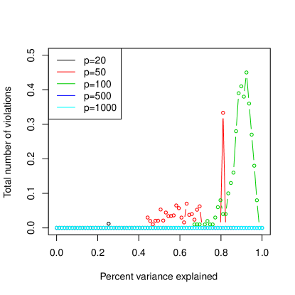
Figure 6: Total number of violations (out of $p$ predictors) of the strong sequential rule, for simulated data with $N=100$ and varying values of $p$. A sequence of models is fit, with decreasing values of $\lambda$ as we move from left to right. The features are uncorrelated. The results are averages over 100 simulations.

Looking at (13), it suggests that if we take a finer grid of $\lambda$ values, there should be fewer violations of the rule. However we have not found this to be true numerically: the average number of violations at each grid point $\lambda$ stays about the same.

5 Screening rules for the elastic net

In the elastic net we solve the problem

$${\rm minimize}\;\frac{1}{2}||\mathbf{y}-\mathbf{X}{\bm{\beta}}||^{2}+\frac{1}{2}\lambda_{2}||{\bm{\beta}}||^{2}+\lambda_{1}||{\bm{\beta}}||_{1}$$ (19)

Letting

$$\mathbf{X}^{*}=\begin{pmatrix}\mathbf{X}\\ \sqrt{\lambda_{2}}\cdot\mathbf{I}\\ \end{pmatrix};\;\;\mathbf{y}^{*}=\begin{pmatrix}\mathbf{y}\\ 0\\ \end{pmatrix},$$ (20)

we can write (19) as

$${\rm minimize}\frac{1}{2}||\mathbf{y}^{*}-\mathbf{X}^{*}{\bm{\beta}}||^{2}+\lambda_{1}||{\bm{\beta}}||_{1}.$$ (21)

In this form we can apply the SAFE rule (2) to obtain a rule for discarding predictors. Now $|{\mathbf{x}_{j}^{*}}^{T}\mathbf{y}^{*}|=|\mathbf{x}_{j}^{T}\mathbf{y}|$, $||\mathbf{x}_{j}^{*}||=\sqrt{||\mathbf{x}_{j}||^{2}+\lambda_{2}}$, $||\mathbf{y}^{*}||=||\mathbf{y}||$. Hence the global rule for discarding predictor $j$ is

$$|\mathbf{x}_{j}^{T}\mathbf{y}|<\lambda_{1}-||\mathbf{y}||\cdot\sqrt{||\mathbf{x}_{j}||^{2}+\lambda_{2}}\cdot\frac{\lambda_{1max}-\lambda_{1}}{\lambda_{1max}}$$ (22)

Note that the glmnet package uses the parametrization $((1-\alpha)\lambda,\alpha\lambda)$ rather than $(\lambda_{2},\lambda_{1})$. With this parametrization the basic SAFE rule has the form

$$|\mathbf{x}_{j}^{T}\mathbf{y}|<\Bigl{(}\alpha\lambda-||\mathbf{y}||\cdot\sqrt{||\mathbf{x}_{j}||^{2}+(1-\alpha)\lambda}\cdot\frac{\lambda_{max}-\lambda}{\lambda_{max}}\Bigr{)}$$ (23)

The strong screening rules turn out to be the same as for the lasso. With the glmnet parametrization the global rule is simply

$$|\mathbf{x}_{j}^{T}\mathbf{y}|<\alpha(2\lambda-\lambda_{max})$$ (24)

while the sequential rule is

$$|\mathbf{x}_{j}^{T}\mathbf{r}|<\alpha(2\lambda-\lambda_{0}).$$ (25)

\psfrag{alpha= 0.1}{$\alpha=0.1$}\psfrag{alpha= 0.5}{$\alpha=0.5$}\psfrag{alpha= 0.9}{$\alpha=0.9$}\includegraphics[width=383.03122pt]{figen.ps}

Figure 7: Elastic net: results for different rules for three different values of the mixing parameter $\alpha$. In the plots, we are fitting along a path of decreasing $\lambda$ values and the plots show the number of predictors left after screening at each stage. The proportion of variance explained by the model is shown along the top of the plot is shown. There were no violations of any of the rules in the 3 scenarios.

Figure 7 show results for the elastic net with standard independent Gaussian data, $n=100,p=1000$, for 3 values of $\alpha$. There were no violations in any of these figures, i.e. no predictor was discarded that had a non-zero coefficient at the actual solution. Again we see that the strong sequential rule performs extremely well, leaving only a small number of excess predictors at each stage.

6 Screening rules for logistic regression

Here we have a binary response $y_{i}=0,1$ and we assume the logistic model

$${\rm Pr}(Y=1|x)=1/(1+\exp(-\beta_{0}-x^{T}\beta))$$ (26)

Letting $p_{i}={\rm Pr}(Y=1|x_{i})$, the penalized log-likelihood is

$$\ell(\beta_{0},{\bm{\beta}})=-\sum_{i}[y_{i}\log p_{i}+(1-y_{i})\log(1-p_{i})]+\lambda||\beta||_{1}$$ (27)

safe derive an exact global rule for discarding predictors, based on the inner products between $\mathbf{y}$ and each predictor, using the same kind of dual argument as in the Gaussian case.

Here we investigate the analogue of the strong rules (5) and (6). The subgradient equation for logistic regression is

$$\mathbf{X}^{T}(\mathbf{y}-\mathbf{p}({\bm{\beta}}))=\lambda\cdot{\rm sign}({\bm{\beta}})$$ (28)

This leads to the global rule: letting $\bar{\mathbf{p}}={\bf 1}\bar{y}$, $\lambda_{max}={\rm max}|\mathbf{x}_{j}^{T}(\mathbf{y}-\bar{\mathbf{p}})|$, we discard predictor $j$ if

$$|\mathbf{x}_{j}^{T}(\mathbf{y}-\bar{\mathbf{p}})|<2\lambda-\lambda_{max}$$ (29)

The sequential version, starting at $\lambda_{0}$, uses $\mathbf{p}_{0}=\mathbf{p}(\hat{\beta}_{0}(\lambda_{0}),\hat{\bm{\beta}}(\lambda_{0}))$:

$$|\mathbf{x}_{j}^{T}(\mathbf{y}-\mathbf{p}_{0})|<2\lambda-\lambda_{0}.$$ (30)

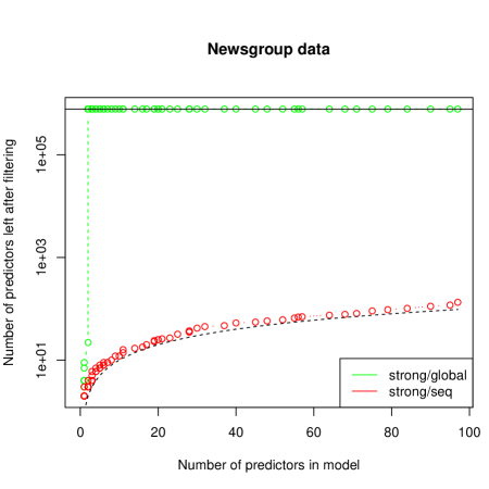
Figure 8: Logistic regression: results for newsgroup example, using the new global rule (29) and the new sequential rule (30). The broken black curve is the 45^o line, drawn on the log scale.

Figure 8 show the result of various rules in an example, the newsgroup document classification problem [lang95:_newsw]. We used the training set cultured from these data by koh07:_l1. The response is binary, and indicates a subclass of topics; the predictors are binary, and indicate the presence of particular tri-gram sequences. The predictor matrix has $0.05\%$ nonzero values. Results for are shown for the new global rule (29) and the new sequential rule (30). We were unable to compute the logistic regression global SAFE rule for this example, using our R language implementation, as this had a very long computation time. But in smaller examples it performed much like the global SAFE rule in the Gaussian case. Again we see that the strong sequential rule (30), after computing the inner product of the residuals with all predictors at each stage, allows us to discard the vast majority of the predictors before fitting. There were no violations of either rule in this example.

Some approaches to penalized logistic regression such as the glmnet package use a weighted least squares iteration within a Newton step. For these algorithms, an alternative approach to discarding predictors would be to apply one of the Gaussian rules within the weighted least squares iteration.

Wu2009 used $|\mathbf{x}_{j}^{T}(\mathbf{y}-\bar{\mathbf{p}})|$ to screen predictors (SNPs) in genome-wide association studies, where the number of variables can exceed a million. Since they only anticipated models with say $k<15$ terms, they selected a small multiple, say $10k$, of SNPs and computed the lasso solution path to $k$ terms. All the screened SNPs could then be checked for violations to verify that the solution found was global.

7 Strong rules for general problems

Suppose that we have a convex problem of the form

$${\rm minimize}_{\bm{\beta}}\Big{[}f({\bm{\beta}})+\lambda\cdot\sum_{k=1}^{K}g({\bm{\beta}}_{j})\Bigr{]}$$ (31)

where $f$ and $g$ are convex functions, $f$ is differentiable and ${\bm{\beta}}=({\bm{\beta}}_{1},{\bm{\beta}}_{2},\ldots{\bm{\beta}}_{K})$ with each ${\bm{\beta}}_{k}$ being a scalar or vector. Suppose further that the subgradient equation for this problem has the form

$$f^{\prime}({\bm{\beta}})+\lambda\cdot\mathbf{s}_{k}=0;\;k=1,2,\ldots K$$ (32)

where each subgradient variable $\mathbf{s}_{k}$ satisfies $||\mathbf{s}_{k}||_{q}\leq A$, and $||\mathbf{s}_{k}||_{q}=A$ when the constraint $g({\bm{\beta}}_{j})=0$ is satisfied (here $||\cdot||_{q}$ is a norm). Suppose that we have two values $\lambda<\lambda_{0}$, and corresponding solutions $\hat{\bm{\beta}}(\lambda),\hat{\bm{\beta}}(\lambda_{0})$. Then following the same logic as in Section 3, we can derive the general strong rule

$$||\frac{f(\hat{\bm{\beta}}_{0k}}{d{\bm{\beta}}_{k}})||_{q}<(1+A)\lambda-A\lambda_{0}$$ (33)

This can be applied either globally or sequentially. In the lasso regression setting, it is easy to check that this reduces to the rules (5),(6) where $A=1$.

The rule (33) has many potential applications. For example in the graphical lasso for sparse inverse covariance estimation [FHT2007], we observe $N$ multivariate normal observations of dimension $p$, with mean $0$ and covariance $\Sigma$, with observed empirical covariance matrix $S$. Letting $\Theta=\Sigma^{-1}$, the problem is to maximize the penalized log-likelihood

$$\log\det\Theta-{\rm tr}(S\Theta)-\lambda||\Theta||_{1},$$ (34)

over non-negative definite matrices $\Theta$. The penalty $||\Theta||_{1}$ sums the absolute values of the entries of $\Theta$; we assume that the diagonal is not penalized. The subgradient equation is

$$\Sigma-S-\lambda\cdot\Gamma=0,$$ (35)

where $\Gamma_{ij}\in{\rm sign}(\Theta_{ij})$. One could apply the rule (33) elementwise, and this would be useful for an optimization method that operates elementwise. This gives a rule of the form $|S_{ij}-\hat{\Sigma}(\lambda_{0})|<2\lambda-\lambda_{0}$. However, the graphical lasso algorithm proceeds in a blockwise fashion, optimizing one whole row and column at a time. Hence for the graphical lasso, it is more effective to discard entire rows and columns at once. For each row $i$, let $s_{12}$, $\sigma_{12}$, and $\Gamma_{12}$ denote $S_{i,-i}$, $\Sigma_{i,-i}$, and $\Gamma_{i,-i}$, respectively. Then the subgradient equation for one row has the form

$$\sigma_{12}-s_{12}-\lambda\cdot\Gamma_{12}=0,$$ (36)

Now given two values $\lambda<\lambda_{0}$, and solution $\hat{\Sigma}^{0}$ at $\lambda_{0}$, we form the sequential rule

$${\rm max}|\hat{\sigma}^{0}_{12}-s_{12}|<2\lambda-\lambda_{0}.$$ (37)

If this rule is satisfied, we discard the entire $i$th row and column of $\Theta$, and hence set them to zero (but retain the $i$th diagonal element). Figure 9 shows an example with $N=100,p=300$, standard independent Gaussian variates. No violations of the rule occurred.

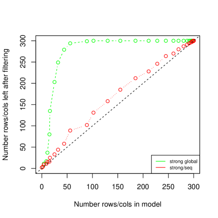
Figure 9: Strong global and sequential rules applied to the graphical lasso. A broken line with unit slope is added for reference.

Finally, we note that strong rules can be derived in a similar way, for other problems such as the group lasso [YL2007]. In particular, if $\mathbf{X}_{\ell}$ denotes the $n\times p_{\ell}$ block of the design matrix corresponding to the features in the $\ell$th group, then the strong sequential rule is simply

$$||\mathbf{X}_{\ell}^{T}\mathbf{r}||_{2}<2\lambda-\lambda_{\max}.$$

When this holds, we set $\boldsymbol{\beta}_{\ell}=\boldsymbol{0}$.

8 Implementation and numerical studies

The strong sequential rule (6) can be used to provide potential speed improvements in convex optimization problems. Generically, given a solution $\hat{\bm{\beta}}(\lambda_{0})$ and considering a new value $\lambda<\lambda_{0}$, let $S(\lambda)$ be the indices of the predictors that survive the screening rule (6): we call this the strong set. Denote by $E$ the eligible set of predictors. Then a useful strategy would be

1. Set $E=S(\lambda)$.

2. Solve the problem at value $\lambda$ using only the predictors in $E$.

3. Check the KKT conditions at this solution for all predictors. If there are no violations, we are done. Otherwise add the predictors that violate the KKT conditions to the set $E$, and repeat steps (b) and (c).

Depending on how the optimization is done in step (b), this can be quite effective. Now in the glmnet procedure, coordinate descent is used, with warm starts over a grid of decreasing values of $\lambda$. In addition, an “ever-active” set of predictors $A(\lambda)$ is maintained, consisting of the indices of all predictors that have a non-zero coefficient for some $\lambda^{\prime}$ greater than the current value $\lambda$ under consideration. The solution is first found for this active set: then the KKT conditions are checked for all predictors. if there are no violations, then we have the solution at $\lambda$; otherwise we add the violators into the active set and repeat.

The two strategies above are very similar, with one using the strong set $S(\lambda)$ and the other using the ever-active set $A(\lambda)$. Figure 10 shows the active and strong sets for an example.

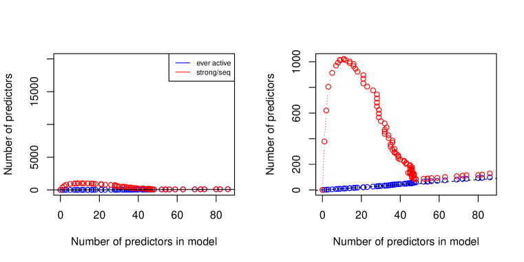
Figure 10: Gaussian lasso setting, $N=200,p=20,000$, pairwise correlation between features of $0.7$. The first 50 predictors have positive, decreasing coefficients. Shown are the number of predictors left after applying the strong sequential rule (6) and the number that have ever been active (i.e. had a non-zero coefficient in the solution) for values of $\lambda$ larger than the current value. A broken line with unit slope is added for reference. The right-hand plot is a zoomed version of the left plot.

Although the strong rule greatly reduces the total number of predictors, it contains more predictors than the ever-active set; accordingly, violations occur more often in the ever-active set than the strong set. This effect is due to the high correlation between features and the fact that the signal variables have coefficients of the same sign. It also occurs with logistic regression with lower correlations, say 0.2.

In light of this, we find that using both $A(\lambda)$ and $S(\lambda)$ can be advantageous. For glmnet we adopt the following combined strategy:

1. Set $E=A(\lambda)$.

2. Solve the problem at value $\lambda$ using only the predictors in $E$.

3. Check the KKT conditions at this solution for all predictors in $S(\lambda)$. If there are violations, add these predictors into $E$, and go back to step (a) using the current solution as a warm start.

4. Check the KKT conditions for all predictors. If there are no violations, we are done. Otherwise add these violators into $A(\lambda)$, recompute $S(\lambda)$ and go back to step (a) using the current solution as a warm start.

Note that violations in step (c) are fairly common, while those in step (d) are rare. Hence the fact that the size of $S(\lambda)$ is $\ll p$ can make this an effective strategy.

We implemented this strategy and compare it to the standard glmnet algorithm in a variety of problems, shown in Tables 1–3. Details are given in the table captions. We see that the new strategy offers a speedup factor of five or more in some cases, and never seems to slow things down.

The strong sequential rules also have the potential for space savings. With a large dataset, one could compute the inner products $\{\mathbf{x}_{j}^{T}\mathbf{r}\}_{1}^{p}$ offline to determine the strong set of predictors, and then carry out the intensive optimization steps in memory using just this subset of the predictors.

9 Discussion

In this paper we have proposed strong global and sequential rules for discarding predictors in statistical convex optimization problems such as the lasso. When combined with checks of the KKT conditions, these can offer substantial improvements in speed while still yielding the exact solution. We plan to include these rules in a future version of the glmnet package.

The RECSAFE method uses the solution at a given point $\lambda_{0}$ to derive a rule for discarding predictors at $\lambda<\lambda_{0}$. Here is another way to (potentially) apply the SAFE rule in a sequential manner. Suppose that we have $\hat{\bm{\beta}}_{0}=\hat{\bm{\beta}}(\lambda_{0})$, and $\mathbf{r}=\mathbf{y}-\mathbf{X}\hat{\bm{\beta}}_{0}$, and we consider the fit at $\lambda<\lambda_{0}$, with $\mathbf{r}=\mathbf{y}-\mathbf{X}\hat{\bm{\beta}}_{0}$. Defining

$$\lambda_{0} = {\rm max}_{j}(|\mathbf{x}_{j}^{T}\mathbf{r}|);$$ (38)

we discard predictor $j$ if

$$|\mathbf{x}_{j}^{T}\mathbf{r}|<\lambda-||\mathbf{r}|||\mathbf{x}_{j}||\frac{\lambda_{0}-\lambda}{\lambda_{0}}$$ (39)

We have been unable to prove the correctness of this rule, and do not know if it is infallible. At the same time, we have been not been able to find a numerical example in which it fails.

Acknowledgements: We thank Stephen Boyd for his comments, and Laurent El Ghaoui and his co-authors for sharing their paper with us before publication, and for helpful feedback on their work. The first author was supported by National Science Foundation Grant DMS-9971405 and National Institutes of Health Contract N01-HV-28183.

Table 1: Glmnet timings (seconds) for fitting a lasso problem in the Gaussian setting. In the first four columns, there are $p=100,000$ predictors, $N=200$ observations, 30 nonzero coefficients, with the same value and signs alternating; signal-to-noise ratio equal to 3. In the rightmost column, the data matrix is sparse, consisting of just zeros and ones, with $0.1\%$ of the values equal to 1. There are $p=50,000$ predictors, $N=500$ observations, with 25% of the coefficients nonzero, having a Gaussian distribution; signal-to-noise ratio equal to 4.3.

Method Population correlation 0.0 0.25 0.5 0.75 Sparse glmnet 4.07 6.13 9.50 17.70 4.14 with seq-strong 2.50 2.54 2.62 2.98 2.52

Table 2: Glmnet timings (seconds) for fitting an elastic net problem. There are $p=100,000$ predictors, $N=200$ observations, 30 nonzero coefficients, with the same value and signs alternating; signal-to-noise ratio equal to 3

Method $\alpha$ 1.0 0.5 0.2 0.1 0.01 glmnet 9.49 7.98 5.88 5.34 5.26 with seq-strong 2.64 2.65 2.73 2.99 5.44

Table 3: Glmnet timings (seconds) fitting a lasso/logistic regression problem. Here the data matrix is sparse, consisting of just zeros and ones, with $0.1\%$ of the values equal to 1. There are $p=50,000$ predictors, $N=800$ observations, with 30% of the coefficients nonzero, with the same value and signs alternating; Bayes error equal to 3%.

Method Population correlation 0.0 0.5 0.8 glmnet 11.71 12.41 12.69 with seq-strong 6.31 9.491 12.86

References

- [1] \harvarditemCandes \harvardand Plan2009nearideal Candes, E. J. \harvardand Plan, Y. \harvardyearleft2009\harvardyearright, ‘Near-ideal model selection by minimization’, Annals of Statistics 37(5), 2145–2177.
- [2] \harvarditem[Efron et al.]Efron, Hastie, Johnstone \harvardand Tibshirani2004lars Efron, B., Hastie, T., Johnstone, I. \harvardand Tibshirani, R. \harvardyearleft2004\harvardyearright, ‘Least angle regression’, Annals of Statistics 32(2), 407–499.
- [3] \harvarditem[El Ghaoui et al.]El Ghaoui, Viallon \harvardand Rabbani2010safe El Ghaoui, L., Viallon, V. \harvardand Rabbani, T. \harvardyearleft2010\harvardyearright, Safe feature elimination in sparse supervised learning, Technical Report UC/EECS-2010-126, EECS Dept., University of California at Berkeley.
- [4] \harvarditemFan \harvardand Lv2008FL2008 Fan, J. \harvardand Lv, J. \harvardyearleft2008\harvardyearright, ‘Sure independence screening for ultra-high dimensional feature space’, Journal of the Royal Statistical Society Series B, to appear .
- [5] \harvarditem[Friedman et al.]Friedman, Hastie, Hoefling \harvardand Tibshirani2007FHT2007 Friedman, J., Hastie, T., Hoefling, H. \harvardand Tibshirani, R. \harvardyearleft2007\harvardyearright, ‘Pathwise coordinate optimization’, Annals of Applied Statistics 2(1), 302–332.
- [6] \harvarditemFuchs2005fuchs Fuchs, J. \harvardyearleft2005\harvardyearright, ‘Recovery of exact sparse representations in the presense of noise’, IEEE Transactions on Information Theory 51(10), 3601–3608.
- [7] \harvarditem[Koh et al.]Koh, Kim \harvardand Boyd2007koh07:_l1 Koh, K., Kim, S.-J. \harvardand Boyd, S. \harvardyearleft2007\harvardyearright, ‘An interior-point method for large-scale l1-regularized logistic regression’, Journal of Machine Learning Research 8, 1519–1555.
- [8] \harvarditemLang1995lang95:_newsw Lang, K. \harvardyearleft1995\harvardyearright, Newsweeder: Learning to filter netnews., in ‘Proceedings of the Twenty-First International Conference on Machine Learning (ICML)’, pp. 331–339.
- [9] \harvarditemMeinhausen \harvardand Buhlmann2006lassograph Meinhausen, N. \harvardand Buhlmann, P. \harvardyearleft2006\harvardyearright, ‘High-dimensional graphs and variable selection with the lasso’, Annals of Statistics 34, 1436–1462.
- [10] \harvarditemTibshirani1996lasso Tibshirani, R. \harvardyearleft1996\harvardyearright, ‘Regression shrinkage and selection via the lasso’, Journal of the Royal Statistical Society Series B 58(1), 267–288.
-
[11]
\harvarditemTibshirani \harvardand Taylor2010genlasso
Tibshirani, R. \harvardand Taylor, J. \harvardyearleft2010\harvardyearright, The solution path of the generalized lasso.
Submitted.
\harvardurlhttp://www-stat.stanford.edu/~ryantibs/papers/genlasso.pdf - [12] \harvarditemTropp2006tropp Tropp, J. \harvardyearleft2006\harvardyearright, ‘Just relax: Convex programming methods for identifying sparse signals in noise’, IEEE Transactions on Information Theory 3(52), 1030–1051.
- [13] \harvarditemWainwright2006sharpthresh Wainwright, M. \harvardyearleft2006\harvardyearright, Sharp thresholds for high-dimensional and noisy sparsity recovery using -constrained quadratic programming (lasso), Technical report, Statistics and EECS Depts., University of California at Berkeley.
- [14] \harvarditem[Wu et al.]Wu, Chen, Hastie, Sobel \harvardand Lange2009Wu2009 Wu, T. T., Chen, Y. F., Hastie, T., Sobel, E. \harvardand Lange, K. \harvardyearleft2009\harvardyearright, ‘Genomewide association analysis by lasso penalized logistic regression’, Bioinformatics 25(6), 714–721.
- [15] \harvarditemYuan \harvardand Lin2007YL2007 Yuan, M. \harvardand Lin, Y. \harvardyearleft2007\harvardyearright, ‘Model selection and estimation in regression with grouped variables’, Journal of the Royal Statistical Society, Series B 68(1), 49–67.
- [16] \harvarditemZhao \harvardand Yu2006lassomodel Zhao, P. \harvardand Yu, B. \harvardyearleft2006\harvardyearright, ‘On model selection consistency of the lasso’, Journal of Machine Learning Research 7, 2541–2563.
- [17] \harvarditemZou \harvardand Hastie2005ZH2005 Zou, H. \harvardand Hastie, T. \harvardyearleft2005\harvardyearright, ‘Regularization and variable selection via the elastic net’, Journal of the Royal Statistical Society Series B. 67(2), 301–320.
- [18]