Time reparametrization invariance in arbitrary range p-spin models: symmetric versus non-symmetric dynamics

Abstract

We explore the existence of time reparametrization symmetry in p-spin models. Using the Martin-Siggia-Rose generating functional, we analytically probe the long-time dynamics. We perform a renormalization group analysis where we systematically integrate over short timescale fluctuations. We find three families of stable fixed points and study the symmetry of those fixed points with respect to time reparametrizations. One of those families is composed entirely of symmetric fixed points, which are associated with the low temperature dynamics. The other two families are composed entirely of non-symmetric fixed points. One of these two non-symmetric families corresponds to the high temperature dynamics.

Time reparametrization symmetry is a continuous symmetry that is spontaneously broken in the glass state and we argue that this gives rise to the presence of Goldstone modes. We expect the Goldstone modes to determine the properties of fluctuations in the glass state, in particular predicting the presence of dynamical heterogeneity.

1 Introduction

Very slow dynamics is an essential feature of glasses [1]. In both structural glasses and spin glasses slow dynamics is manifested through a dramatic increase in relaxation times. This slowdown has been captured in mean field theories, such as the mode coupling theory for supercooled liquids [2] and the dynamical theory for mean field spin glass models [3, 4, 5, 6]. Even though mean field theories are useful in describing some aspects of glassy dynamics, they do not completely capture phenomena associated with fluctuations. Fluctuations have been shown, particularly with the discovery of dynamical heterogeneities, to be central to an understanding of glassy dynamics [7].

Dynamical heterogeneities - mesoscopic regions that evolve differently from each other as well as from the bulk - have been found in experimental studies of materials close to the glass transition [8, 9, 10] and in simulations of both spin glasses and structural glasses [11, 12, 13]. Their presence has been directly observed at the microscopic level in experiments on colloidal glasses [10] and granular systems [14]. Understanding the onset of heterogeneities without an apparent structural trigger is believed to be key to an understanding of the glass transition [7]. There have been several theoretical attempts to explain the emergence of heterogeneous dynamics as the glass transition is approached. One of them is a geometrical picture, according to which dynamical heterogeneities result from non-trivial structure in the space of trajectories due to dynamical constraints [15]. Another proposed explanation is provided by the Random First Order transition (RFOT) approach, in which a liquid freezes into a mosaic of aperiodic crystals [16]. Here we will explore a different theoretical avenue to explain dynamical heterogeneities, which is based on time reparametrization symmetry [17, 18, 19].

Time reparametrization symmetry (TRS), the invariance under transformations of the time variable $t\rightarrow h(t)$, was discovered some years ago in the mean-field non-equilibrium dynamics of the Sherrington-Kirkpatrick model and the p-spin model [5, 6]. The symmetry, which was shown to be present in the long-time limit of the mean field evolution, implies that the asymptotic equations do not have a unique solution [5, 6, 20]. In more recent studies, TRS has been proved to be present in the long time dynamics of the glass state in a short range spin glass model, the Edwards-Anderson model [17, 18, 19]. In this last case, the proof of the symmetry is at the level of the generating functional, including all fluctuations. Using the renormalization group (RG), it was shown that the stable fixed point of the generating functional corresponding to glassy dynamics is invariant under reparametrizations of the time variable. However not all models of interacting spins under Langevin dynamics show this behavior. For example, in a study of the O(N) model it was shown that the symmetry is not present, even for the long time limit of the low temperature dynamics [25]. The explanation for dynamical heterogeneities from TRS is derived from the fact that TRS is spontaneously broken by the correlations and responses in the glass state. A spontaneously broken continuous symmetry is expected to give rise to Goldstone modes, and these modes are associated with spatially correlated fluctuations of the time variable, which give rise to heterogeneous dynamics. The proposal that dynamical heterogeneities originate in reparametrization fluctuations of the time variable is supported by positive evidence from numerical studies in spin glasses [18] and in structural glasses [23, 24].

In the present work we go beyond mean field theory and use a renormalization group procedure to study the presence of time reparametrization symmetry in the long time dynamics of p-spin models with arbitrary interaction range, including all fluctuations. We consider a system of soft spins on a lattice, with p-spin interactions. The spin couplings are assumed to be uncorrelated Gaussian random variables with zero mean. We assume Langevin dynamics for the spins with a white noise term that represents the coupling of the spins to a heat reservoir. We set up the calculation by writing the generating functional of the spin correlations and responses using the Martin-Siggia-Rose (MSR) approach and introduce two-time fields that are associated with the spin correlations and responses. To study the long time dynamics we start the renormalization group procedure by introducing a short time cutoff $\tau_{0}$. We systematically increase the short time cutoff by integrating over the two-time fields associated with the shortest time differences, thus following a procedure analogous to Wilson’s approach to the RG. In our case, however, we integrate over fluctuations that are fast in time, not in space. We find three families of stable fixed points. The first family corresponds to fixed point actions containing the coupling to the thermal bath but not the spin-spin interactions. The fixed points in this family are not time reparametrization invariant, and we believe that this family is associated with the high temperature dynamics. A second family of stable fixed points that are not time reparametrization invariant corresponds to fixed point actions containing both the coupling to the thermal bath and the spin-spin interactions. For the third family, the spin-spin interaction term is marginal but the coupling to the thermal bath is irrelevant. The fixed points in this last family are time reparametrization invariant, and we believe that they represent the low temperature glassy dynamics of the model. After obtaining these results, we discuss their connection with dynamical heterogeneity in the p-spin model, and we speculate on how a similar procedure may be applied to models of structural glasses, which have been shown to be connected to the p-spin model [21, 22].

The rest of the paper is organized as follows: in Sec. 2 we start by giving a description of the model and an illustration of how we derive the Martin-Siggia-Rose generating functional; in Sec. 3 we show how we use Wilson’s approach to the renormalization group to get stable fixed points; in Sec. 4 we study the stable fixed point generating functionals and determine which ones are invariant under reparametrizations of the time variable; and in Sec. 5 we end with a discussion of our results and conclusions.

2 Model and MSR generating functional

The p-spin Hamiltonian is given by

$$H=-\frac{1}{p!}\sum_{i_{1}...i_{p}}J_{i_{1}...i_{p}}\phi_{i_{1}}...\phi_{i_{p}},$$ (1)

where the $\{\phi\}_{i=1,\cdots,N}$ are soft spins subject to the spherical constraint $\sum_{i=1}^{N}[\phi_{i}(t)]^{2}=N$, and the couplings are assumed to be uncorrelated, Gaussian distributed, zero mean random variables, $P\{J\}=\prod_{i_{1}<...<i_{p}}\frac{1}{\sqrt{4\pi K_{i_{1}...i_{p}}}}\exp[-J_{i_{1}...i_{p}}^{2}/4K_{i_{1}...i_{p}}]$. The dynamics is given by the Langevin equation

$$\Gamma_{0}^{-1}\partial_{t}\phi_{i}(t)=-\frac{\delta H}{\delta\phi_{i}(t)}+\eta_{i}(t),$$ (2)

where the $\{\eta_{i}(t)\}_{i=1,...,N}$ are assumed to be zero mean gaussian random variables with the correlation $\langle\eta_{i}(t)\eta_{j}(t^{\prime})\rangle=2T\delta_{ij}\delta(t-t^{\prime})$ that couple the spins to a thermal bath at temperature $T$. Then the Langevin equation can be written as

$$\Gamma_{0}^{-1}\partial_{t}\phi_{i}(t)=\frac{p}{p!}\sum_{i_{1}...i_{p-1}}J_{i,i_{1}...i_{p-1}}\phi_{i_{1}}...\phi_{i_{p-1}}+\eta_{i}(t).$$ (3)

From the Langevin equation we use the Martin-Siggia-Rose formalism [26] and write down the noise averaged generating functional

$$\langle Z[\{l_{i}\},\{h_{i}\}]\rangle=\int D\phi D\hat{\phi}D\hat{\varphi}D\hat{N}\exp\left\{L[\phi,\hat{\phi}]+\sum_{i=1}^{N}\int_{t_{0}}^{t_{f}}dt[l_{i}(t)\phi_{i}(t)\right.$$

$$\left.+ih_{i}(t)\hat{\phi}_{i}(t)]+i\sum_{i=1}^{N}\hat{\varphi}_{i}[\phi_{i}(t_{0})-\varphi_{i}]+i\int_{t_{0}}^{t_{f}}dt\hat{N}(t)\left[\sum_{i=1}^{N}\phi_{i}^{2}(t)-N\right]\right\},$$ (4)

where the $l$ and $h$ are sources and the last two terms in the exponent are due to the initial condition and spherical constraint, respectively. The action $L[\phi,\hat{\phi}]$ is given by

$$L[\phi,\hat{\phi}]=-i\sum_{i=1}^{N}\int_{t_{0}}^{t_{f}}dt\;\hat{\phi}_{i}(t) \left[\Gamma_{0}^{-1}\partial_{t}\phi_{i}(t)-iT\hat{\phi}_{i}(t)\right.$$ (5)

$$\left.-\frac{p}{p!}\sum_{i_{1}...i_{p-1}}J_{i,i_{1}...i_{p-1}}\phi_{i_{1}}...\phi_{i_{p-1}}\right].$$

We now average the generating functional over the disorder in the system. The action contains only one term with an explicit dependence on the disorder, which we call $L_{J}[\phi,\hat{\phi}]$,

$$L_{J}[\phi,\hat{\phi}]=i\frac{p}{p!}\sum_{i_{1}...i_{p}}\int_{t_{0}}^{t_{f}}dtJ_{i_{1}...i_{p}}\hat{\phi}_{i_{1}}(t)\phi_{i_{2}}(t)\cdots\phi_{i_{p}}(t).$$ (6)

We now compute the part of the generating functional affected by disorder averaging,

$$\overline{\exp(L_{J}[\phi,\hat{\phi}])}=\int DJP\{J\}\exp[L_{J}],$$ (7)

with $DJ\equiv\prod\limits_{i_{1}<\cdots<i_{p}}dJ_{i_{1}...i_{p}}$. Therefore, after integrating over the disorder we have $\overline{\exp(L_{J}[\phi,\hat{\phi}])}$ given by

$$\overline{\exp(L_{J}[\phi,\hat{\phi}])}=\exp \left[-\frac{p^{2}}{p!}\sum_{i_{1}...i_{p}}K_{i_{1}...i_{p}}\int_{t_{0}}^{t_{f}}\!\!\int_{t_{0}}^{t_{f}}dtdt^{\prime}\right.$$ (8)

$$\left.\times\!\sum\limits_{\alpha_{i_{r}},\alpha_{i_{r}}^{\prime}\in\{0,1\}}^{C=1,C^{\prime}=1}\sum_{i_{1}...i_{p}}\prod\limits_{r=1}^{p}\phi_{i_{r}}^{\alpha_{i_{r}}}(t)\phi_{i_{r}}^{\alpha_{i_{r}}^{\prime}}(t^{\prime})\right],$$

where we have re-labeled the fields using the definitions $\phi_{i}^{0}(t)\equiv\hat{\phi}_{i}(t)$ and $\phi_{i}^{1}(t)\equiv\phi_{i}(t)$. The constrained variables $C$ and $C^{\prime}$ are given by $C\equiv\sum\limits_{r=1}^{p}(1-\alpha_{i_{r}})$, $C^{\prime}\equiv\sum\limits_{r=1}^{p}(1-\alpha_{i_{r}}^{\prime})$, and the constraints $C=C^{\prime}=1$ enforce the condition that for each of the two times $t$ and $t^{\prime}$, there is a product of fields, of which only one is a $\hat{\phi}$ and all others are $\phi$ fields. We are also interested in introducing two-time fields $Q_{i}^{\alpha,\alpha^{\prime}}(t_{1},t_{2})$, physically associated with two-time correlations and responses. In order to do this we write the number one in terms of an integral of a product of delta functions that enforce the condition $Q_{i}^{\alpha,\alpha^{\prime}}(t_{1},t_{2})=\phi_{i}^{\alpha}(t_{1})\phi_{i}^{\alpha^{\prime}}(t_{2})$,

$$1=\int DQ\prod\limits_{i,t_{1},t_{2}}\prod\limits_{\alpha_{i},\alpha_{i}^{\prime}\in\{0,1\}}\delta\left(Q_{i}^{\alpha_{i},\alpha_{i}^{\prime}}(t_{1},t_{2})-\phi_{i}^{\alpha_{i}}(t_{1})\phi_{i}^{\alpha_{i}^{\prime}}(t_{2})\right).$$ (9)

By writing the delta function in exponential form we get

$$1=\int DQD\hat{Q}\exp \left\{i\sum\limits_{i}\!\sum\limits_{\alpha_{i},\alpha_{i}^{\prime}\in\{0,1\}}\int\int dt_{1}dt_{2}\hat{Q}_{i}^{\overline{\alpha_{i}},\overline{\alpha_{i}^{\prime}}}(t_{1},t_{2})\right.$$ (10)

$$\left.\times\left(Q_{i}^{\alpha_{i},\alpha_{i}^{\prime}}(t_{1},t_{2})-\phi_{i}^{\alpha_{i}}(t_{1})\phi_{i}^{\alpha_{i}^{\prime}}(t_{2})\right)\right\},$$

where we have introduced the auxiliary two-time fields $\hat{Q}_{i}^{\alpha_{i},\alpha_{i}^{\prime}}(t_{1},t_{2})$ and the notation $\overline{0}=1$, $\overline{1}=0$. We now obtain the noise and disorder averaged generating functional

$$\overline{\langle Z[\{l_{i}\},\{h_{i}\}]\rangle}=\int DQD\hat{Q}D\phi^{0}D\phi^{1}D\hat{\varphi}D\hat{N}\exp({\cal S}),$$

$${\cal S}=S_{1}+S_{J}+S_{spin}+S_{ext}+S_{BC}+S_{SC}.$$ (11)

Here we have written the different terms of the action separately:

$$S_{1}[Q,\hat{Q},\phi^{0},\phi^{1}]= i\sum\limits_{i}\!\sum\limits_{\alpha_{i},\alpha_{i}^{\prime}\in\{0,1\}}\int_{t_{0}}^{t_{f}}\!\!\int_{t_{0}}^{t_{f}}dt_{1}dt_{2}\hat{Q}_{i}^{\overline{\alpha_{i}},\overline{\alpha_{i}^{\prime}}}(t_{1},t_{2})$$ (12)

$$\times\left(Q_{i}^{\alpha_{i},\alpha_{i}^{\prime}}(t_{1},t_{2})-\phi_{i}^{\alpha_{i}}(t_{1})\phi_{i}^{\alpha_{i}^{\prime}}(t_{2})\right),$$

$$S_{J}[Q]=-\frac{p^{2}}{p!}\sum_{i_{1}...i_{p}}K_{i_{1}...i_{p}}\int_{t_{0}}^{t_{f}}\!\!\int_{t_{0}}^{t_{f}}dt_{1}dt_{2}\!\sum\limits_{\alpha_{i_{r}},\alpha_{i_{r}}^{\prime}\in\{0,1\}}^{C=1,C^{\prime}=1}\prod\limits_{r=1}^{p}Q_{i_{r}}^{\alpha_{i_{r}},\alpha_{i_{r}}^{\prime}}(t_{1},t_{2}),$$ (13)

$$S_{spin}[\phi^{0},\phi^{1}] = -i\sum_{i=1}^{N}\int_{t_{0}}^{t_{f}}dt\phi^{0}_{i}(t)\left[\Gamma^{-1}\partial_{t}\phi^{1}_{i}(t)+\gamma_{00}\phi^{0}_{i}(t)\right]-\frac{p^{2}}{p!}\sum_{i_{1}...i_{p}}K_{i_{1}...i_{p}}$$ (14)

$$\times\int_{t_{0}}^{t_{f}}\!\!\int_{t_{0}}^{t_{f}}dt_{1}dt_{2}g(t_{1}-t_{2})\!\sum\limits_{\alpha_{i_{r}},\alpha_{i_{r}}^{\prime}\in\{0,1\}}^{C=1,C^{\prime}=1}\prod\limits_{r=1}^{p}\phi_{i_{r}}^{\alpha_{i_{r}}}(t_{1})\phi_{i_{r}}^{\alpha_{i_{r}}^{\prime}}(t_{2}),$$

$$S_{ext}[\phi^{0},\phi^{1};l,h]=\int_{t_{0}}^{t_{f}}dt\left[l_{i}(t)\phi^{0}_{i}(t)+ih_{i}(t)\phi^{1}_{i}(t)\right],$$ (15)

$$S_{BC}[\phi^{1},\hat{\varphi};\varphi]=i\sum_{i=1}^{N}\hat{\varphi}_{i}\left[\phi^{1}_{i}(t_{0})-\varphi_{i}\right],$$ (16)

$$S_{SC}[\phi^{1},\hat{N};N]=i\int_{t_{0}}^{t_{f}}dt\hat{N}(t)\left[\sum_{i=1}^{N}(\phi^{1}_{i}(t))^{2}-N\right],$$ (17)

and we have $\Gamma=\Gamma_{0}$, $\gamma_{00}=-iT$ and $g(t-t^{\prime})=0$ at the start of the RG flow.

3 Renormalization group analysis

3.1 Renormalization Group Transformation

We perform a renormalization group analysis on the time variables. For simplicity we take $t_{0}=0$ and $t_{f}=\infty$ from now on. We focus on the two-time fields. First, we introduce a cutoff in the integration of two-time fields, $\tau_{0}\leq|t_{1}-t_{2}|$. We then write the terms of the action affected by the cutoff:

$$S_{1}[Q,\hat{Q}]= i\sum\limits_{i}\int\limits_{0\leq t_{1},t_{2}<\infty\atop\tau_{0}\leq|t_{1}-t_{2}|}dt_{1}dt_{2}\!\sum\limits_{\alpha_{i},\alpha_{i}^{\prime}}\hat{Q}_{i}^{\overline{\alpha_{i}},\overline{\alpha_{i}^{\prime}}}(t_{1},t_{2})$$ (18)

$$\times\left(Q_{i}^{\alpha_{i},\alpha_{i}^{\prime}}(t_{1},t_{2})-\phi_{i}^{\alpha_{i}}(t_{1})\phi_{i}^{\alpha_{i}^{\prime}}(t_{2})\right),$$

$$S_{J}[Q]=-\frac{p^{2}}{p!}\sum_{i_{1}...i_{p}}K_{i_{1}...i_{p}}\int\limits_{0\leq t_{1},t_{2}<\infty\atop\tau_{0}\leq|t_{1}-t_{2}|}dt_{1}dt_{2}\!\sum\limits_{\alpha_{i_{r}},\alpha_{i_{r}}^{\prime}\in\{0,1\}}^{C=1,C^{\prime}=1}\prod\limits_{r=1}^{p}Q_{i_{r}}^{\alpha_{i_{r}},\alpha_{i_{r}}^{\prime}}(t_{1},t_{2}).$$ (19)

We define fast and slow fields respectively by $Q_{>i}^{\alpha_{i},\alpha_{i}^{\prime}}(t_{1},t_{2})=Q_{i}^{\alpha_{i},\alpha_{i}^{\prime}}(t_{1},t_{2})$, for $\tau_{0}\leq|t_{1}-t_{2}|<b\tau_{0}$ and $Q_{<i}^{\alpha_{i},\alpha_{i}^{\prime}}(t_{1},t_{2})=Q_{i}^{\alpha_{i},\alpha_{i}^{\prime}}(t_{1},t_{2})$, for $b\tau_{0}\leq|t_{1}-t_{2}|$, with $b>1$. This separation of fast and slow parts of the fields results in a separation in the terms:

$$S_{1}[Q,\hat{Q},\phi^{0},\phi^{1}] = S_{1}[Q_{>},\hat{Q}_{>},\phi^{0},\phi^{1}]+S_{1}[Q_{<},\hat{Q}_{<},\phi^{0},\phi^{1}],$$ (20)

$$S_{J}[Q] = S_{J}[Q_{>}]+S_{J}[Q_{<}].$$ (21)

Next we calculate the integral $I_{>}$ over fast fields. To do this we use the fact that there are no cross-terms between fast and slow fields in the integral:

$$I_{>}=\int DQ_{>}D\hat{Q}_{>}\exp\left\{i\sum\limits_{i}\int\limits_{\tau_{0}\leq|t_{1}-t_{2}|<b\tau_{0}\atop 0\leq t_{1},t_{2}<\infty}dt_{1}dt_{2}\!\sum\limits_{\alpha_{i},\alpha_{i}^{\prime}}\hat{Q}_{>i}^{\overline{\alpha_{i}},\overline{\alpha_{i}^{\prime}}}(t_{1},t_{2})\right.$$

$$\left.\times\left(Q_{>i}^{\alpha_{i},\alpha_{i}^{\prime}}(t_{1},t_{2})-\phi_{i}^{\alpha_{i}}(t_{1})\phi_{i}^{\alpha_{i}^{\prime}}(t_{2})\right)\right.$$

$$\left.-\frac{p^{2}}{p!}\sum_{i_{1}...i_{p}}K_{i_{1}...i_{p}}\int\limits_{\tau_{0}\leq|t_{1}-t_{2}|<b\tau_{0}\atop 0\leq t_{1},t_{2}<\infty}dt_{1}dt_{2}\!\sum\limits_{\alpha_{i_{r}},\alpha_{i_{r}}^{\prime}\in\{0,1\}}^{C=1,C^{\prime}=1}\prod\limits_{r=1}^{p}Q_{>i_{r}}^{\alpha_{i_{r}},\alpha_{i_{r}}^{\prime}}(t_{1},t_{2})\right\}.$$ (22)

Calculating the integral over the ${Q}_{>}$ fields constitutes undoing the delta function integral transformation we used to introduce the two-time fields for the fast modes. Hence,

$$I_{>}=\exp\left\{-\frac{p^{2}}{p!}\sum_{i_{1}...i_{p}}K_{i_{1}...i_{p}}\int\limits_{\tau_{0}\leq|t_{1}-t_{2}|<b\tau_{0}\atop 0\leq t_{1},t_{2}<\infty}dt_{1}dt_{2}\!\sum\limits_{\alpha_{i_{r}},\alpha_{i_{r}}^{\prime}\in\{0,1\}}^{C=1,C^{\prime}=1}\prod\limits_{r=1}^{p}\phi_{i_{r}}^{\alpha_{i_{r}}}(t_{1})\phi_{i_{r}}^{\alpha_{i_{r}}^{\prime}}(t_{2})\right\}.$$ (23)

Next we re-scale all the one-time and two-time fields, thus restoring the cutoff to its original value $\tau_{0}$

$$Q_{<i}^{\alpha_{i},\alpha_{i}^{\prime}}(bt^{\prime}_{1},bt^{\prime}_{2})=b^{\lambda_{\alpha_{i}\alpha_{i}^{\prime}}}{Q^{\prime}}_{i}^{\alpha_{i},\alpha_{i}^{\prime}}(t^{\prime}_{1},t^{\prime}_{2}),$$ (24)

$$\hat{Q}_{<i}^{\alpha_{i},\alpha_{i}^{\prime}}(bt^{\prime}_{1},bt^{\prime}_{2})=b^{\hat{\lambda}_{\alpha_{i}\alpha_{i}^{\prime}}}{\hat{Q^{\prime}}}_{i}^{\alpha_{i},\alpha_{i}^{\prime}}(t^{\prime}_{1},t^{\prime}_{2}),$$ (25)

$$bt^{\prime}=t,$$ (26)

$$\phi_{i}^{\alpha_{i}}(bt^{\prime})=b^{\lambda_{\alpha_{i}}}{\phi^{\prime}}_{i}^{\alpha_{i}}(t^{\prime}),$$ (27)

$$l_{i}(bt^{\prime})=b^{\lambda_{l}}l^{\prime}_{i}(t^{\prime}),$$ (28)

$$h_{i}(bt^{\prime})=b^{\lambda_{h}}h^{\prime}_{i}(t^{\prime}),$$ (29)

$$\hat{\varphi}_{i}=b^{\lambda_{\varphi}}\hat{\varphi}^{\prime}_{i}.$$ (30)

From the definition of the two time fields in Eq. (9) and the transformations of the fields we have

$$\lambda_{\alpha_{i},\alpha_{i}^{\prime}}=\lambda_{\alpha_{i}}+\lambda_{\alpha_{i}^{\prime}}.$$ (31)

By rescaling the fields in the part of the action arising from the disorder average ($S_{J}$) we get

$$S^{\prime}_{J}[Q]= -\frac{p^{2}}{p!}b^{\lambda_{J}}\sum_{i_{1}...i_{p}}K_{i_{1}...i_{p}}\int\limits_{\tau_{0}\leq|b(t_{1}^{\prime}-t_{2}^{\prime})|}dt_{1}^{\prime}dt_{2}^{\prime}$$ (32)

$$\times\!\sum\limits_{\alpha_{i_{r}},\alpha_{i_{r}}^{\prime}\in\{0,1\}}^{C=1,C^{\prime}=1}\sum_{i_{1}...i_{p}}\prod\limits_{r=1}^{p}{Q^{\prime}}_{i_{r}}^{\alpha_{i_{r}},\alpha_{i_{r}}^{\prime}}(t_{1}^{\prime},t_{2}^{\prime}).$$

Using the relation between $\lambda_{\alpha,\alpha^{\prime}}$, $\lambda_{\alpha}$ and $\lambda_{\alpha^{\prime}}$ given by Eq. (31) together with the constraints $C=C^{\prime}=1$ we get

$$\lambda_{J}\equiv 2\lambda_{0}+2(p-1)\lambda_{1}+2.$$ (33)

The other important term we need to consider is $S_{spin}$. When we rescale the fields we obtain

$$S^{\prime}_{spin}[\phi^{0},\phi^{1}]=-i\sum_{i=1}^{N}\int_{0}^{\infty}dt^{\prime}{\phi^{\prime}}^{0}_{i}(t^{\prime})\left[b^{\lambda_{vel}}\Gamma^{-1}\partial_{t^{\prime}}{\phi^{\prime}}^{1}_{i}(t^{\prime})+b^{\lambda_{T}}\gamma_{00}{\phi^{\prime}}^{0}_{i}(t^{\prime})\right]$$ (34)

$$-\frac{p^{2}}{p!}\sum_{i_{1}...i_{p}}K_{i_{1}...i_{p}}\int\!\!\int_{0}^{\infty}dt_{1}^{\prime}dt_{2}^{\prime}b^{\lambda_{J}}g(t_{1}^{\prime}-t_{2}^{\prime})\!\sum\limits_{\alpha_{i_{r}},\alpha_{i_{r}}^{\prime}\in\{0,1\}}^{C=1,C^{\prime}=1}\prod\limits_{r=1}^{p}{\phi^{\prime}}_{i_{r}}^{\alpha_{i_{r}}}(t_{1}^{\prime}){\phi^{\prime}}_{i_{r}}^{\alpha_{i_{r}}^{\prime}}(t_{2}^{\prime})$$

The result is the following set of flow equations

$$\Gamma^{-1}\rightarrow\Gamma^{{}^{\prime}-1}=\Gamma^{-1}b^{\lambda_{vel}},$$ (35)

$$\gamma_{00}\rightarrow\gamma^{\prime}_{00}=\gamma_{00}b^{\lambda_{T}},$$ (36)

$$g(t_{1}-t_{2})\rightarrow g^{\prime}(t_{1}^{\prime}-t_{2}^{\prime})=b^{\lambda_{J}}\left(g(b(t_{1}^{\prime}-t_{2}^{\prime}))+{\cal C}_{\tau_{0}\leq|bt^{\prime}_{1}-bt^{\prime}_{2}|<b\tau_{0}}\right),$$ (37)

where ${\cal C}_{\cal P}$ is defined by ${\cal C}_{\cal P}=1$ if ${\cal P}$ is true and ${\cal C}_{\cal P}=0$ if ${\cal P}$ is not true, and

$$\lambda_{vel}=\lambda_{0}+\lambda_{1},$$ (38)

$$\lambda_{T}=1+2\lambda_{0}.$$ (39)

If we let $b=e^{dl}\cong 1+dl$ then the flow equations for $\Gamma$ and $\gamma_{00}$ can be written

$$\frac{d\Gamma}{dl}=-\lambda_{vel}\Gamma,$$ (40)

$$\frac{d\gamma_{00}}{dl}=\lambda_{T}\gamma_{00}.$$ (41)

The terms that are left to consider are the constraint terms $S_{1}$ and $S_{SC}$, the boundary condition term $S_{BC}$, and the coupling to the sources $S_{ext}$. Physically we expect that the constraints represented by $S_{1}$ and $S_{SC}$ will still be valid in the long time limit, and therefore those terms should be marginal. This leads to the equations $\hat{\lambda}_{\overline{\alpha_{i}},\overline{\alpha_{i}^{\prime}}}=-2-\lambda_{\alpha_{i},\alpha_{i}^{\prime}}=-2-\lambda_{\alpha_{i}}-\lambda_{\alpha_{i}^{\prime}}$ and $\lambda_{N}=-1$ respectively. It is not obvious from physical considerations alone what the behavior of the boundary condition and the coupling to the sources should be. The exponents $\lambda_{l}$, $\lambda_{h}$, $\lambda_{\varphi}$ control their scaling behavior, and could in principle be chosen to make the terms marginal, but they do not play any role in what follows.

In order to determine the nature of the fixed points, we need to choose values for the scaling exponents $\lambda_{0}$ and $\lambda_{1}$.

3.2 Choice of Scaling Exponents

In traditional RG calculations one determines an engineering dimension for the field variable by requiring that the free theory action be marginal. In our case none of the terms in the action is of the same form as the gradient squared term that is usually considered to be the unperturbed part of the action and assumed to be marginal. The only systematic way to proceed is to consider what happens when each of the terms in the action is marginal. We start by noting that the presence of the spherical constraint $\sum_{i=1}^{N}[\phi_{i}(t)]^{2}=N$ implies that there is an upper bound on the correlation function $C(t,t^{\prime})\sim Q^{11}(t,t^{\prime})$, and therefore we must have the constraint $\lambda_{1}\leq 0$. The case of $\lambda_{1}=0$ corresponds to freezing and the strict inequality corresponds to a decaying correlation. The terms in the action that are of interest for our analysis are the three terms contained in $S_{spin}$: the spin-spin interaction, the term containing a time derivative and the term coupling the system to the thermal bath. As indicated in Eqs. (33), (38) and (39), those three terms have the scaling exponents $\lambda_{J}=2(1+\lambda_{0}+(p-1)\lambda_{1})$, $\lambda_{vel}=\lambda_{0}+\lambda_{1}$ and $\lambda_{T}=1+2\lambda_{0}$, respectively. By considering the cases in which only one of the terms is marginal we get the results summarized in Fig. 1.

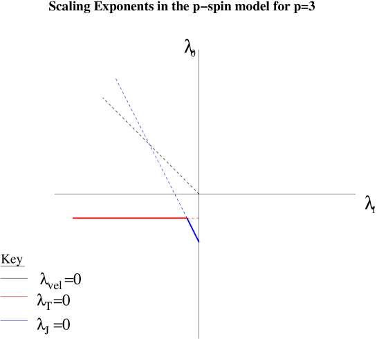
Figure 1: The figure shows the different lines along which each one of the three terms in $S_{spin}$ is marginal for $p=3$. The red line corresponds to a marginal coupling to the thermal bath ($\lambda_{T}=0$), the black line corresponds to a marginal time-derivative term ($\lambda_{vel}=0$), and the blue line corresponds to a marginal spin-spin interaction term ($\lambda_{J}=0$).

In the case in which the coupling to the thermal bath is marginal, we have a line $\lambda_{0}=-1/2$ in the ($\lambda_{1}$, $\lambda_{0}$) plane. Considering the constraint $\lambda_{1}\leq 0$ and the values of $\lambda_{J}$ and $\lambda_{vel}$ we find that there is an interval on this line, $\lambda_{1}<\frac{-1}{2(p-1)}$, in which both the spin-spin interactions and the time derivative term are irrelevant. Since the coupling to the thermal bath is marginal then we have a family of stable high temperature fixed points. Second, we consider the case where the time derivative term is marginal, corresponding to the line $\lambda_{0}=-\lambda_{1}$ in the ($\lambda_{1}$, $\lambda_{0}$) plane. Since we have $\lambda_{1}\leq 0$, the exponent $\lambda_{T}$ of Eq. (39) is always positive, i.e. the coupling to the thermal bath is always a relevant perturbation. Thus the fixed points that contain only the time derivative term are always unstable. We then consider the case where the spin-spin term is marginal. This happens on the line described by $\lambda_{0}=-1-(p-1)\lambda_{1}$. In the interval $\frac{-1}{2(p-1)}<\lambda_{1}\leq 0$ the time derivative term and coupling to the thermal bath are irrelevant. This gives rise to a family of stable low temperature fixed points. Finally, there is the special point $\lambda_{1}=\frac{-1}{2(p-1)},\lambda_{0}=-1/2$, for which both the coupling to the thermal bath and the spin-spin interaction are marginal, but the time derivative term is irrelevant, thus allowing for an additional family of stable fixed points.

The above analysis shows that there is a subset of the ($\lambda_{1}$, $\lambda_{0}$) plane for which a high temperature dynamical fixed point family is present. The effective generating functional for this fixed point family is

$${\cal Z}_{fp}[l,h;T]=\overline{\langle Z[\{l_{i}\},\{h_{i}\}]\rangle}_{fp}=\int DQD\hat{Q}D\phi^{0}D\phi^{1}D\hat{\varphi}D\hat{N}$$

$$\times\exp\left\{i\sum\limits_{i}\int\!\!\int_{0}^{\infty}dt_{1}dt_{2}\!\sum\limits_{\alpha_{i},\alpha_{i}^{\prime}}\hat{Q}_{i}^{\overline{\alpha_{i}},\overline{\alpha_{i}^{\prime}}}(t_{1},t_{2})\left(Q_{i}^{\alpha_{i},\alpha_{i}^{\prime}}(t_{1},t_{2})-\phi_{i}^{\alpha_{i}}(t_{1})\phi_{i}^{\alpha_{i}^{\prime}}(t_{2})\right)\right.$$

$$-T\sum\limits_{i=1}^{N}\int_{0}^{\infty}dt\left(\phi_{i}^{0}(t)\right)^{2}$$

$$\left.+\int_{0}^{\infty}dt[l_{i}(t)\phi^{0}_{i}(t)+ih_{i}(t)\phi^{1}_{i}(t)]\right.$$

$$\left.+i\sum_{i=1}^{N}\hat{\varphi}_{i}[\phi^{1}_{i}(t_{0})-\varphi_{i}]+i\int_{0}^{\infty}dt\hat{N}(t)\left[\sum_{i=1}^{N}(\phi^{1}_{i}(t))^{2}-N\right]\right\}.$$ (42)

There is another subset of the ($\lambda_{1}$, $\lambda_{0}$) plane for which a low temperature interaction-dominated fixed point family is present. The effective generating functional for this family of fixed points is

$${\cal Z}_{fp}[l,h;J]=\overline{\langle Z[\{l_{i}\},\{h_{i}\}]\rangle}_{fp}=\int DQD\hat{Q}D\phi^{0}D\phi^{1}D\hat{\varphi}D\hat{N}$$

$$\times\exp\left\{i\sum\limits_{i}\int\!\!\int_{0}^{\infty}dt_{1}dt_{2}\!\sum\limits_{\alpha_{i},\alpha_{i}^{\prime}}\hat{Q}_{i}^{\overline{\alpha_{i}},\overline{\alpha_{i}^{\prime}}}(t_{1},t_{2})\left(Q_{i}^{\alpha_{i},\alpha_{i}^{\prime}}(t_{1},t_{2})-\phi_{i}^{\alpha_{i}}(t_{1})\phi_{i}^{\alpha_{i}^{\prime}}(t_{2})\right)\right.$$

$$\left.-\frac{p^{2}}{p!}\sum_{i_{1}...i_{p}}K_{i_{1}...i_{p}}\int\!\!\int_{0}^{\infty}dt_{1}dt_{2}\!\sum\limits_{\alpha_{i_{r}},\alpha_{i_{r}}^{\prime}\in\{0,1\}}^{C=1,C^{\prime}=1}\prod\limits_{r=1}^{p}Q_{i_{r}}^{\alpha_{i_{r}},\alpha_{i_{r}}^{\prime}}(t_{1},t_{2})\right.$$

$$\left.+\int_{0}^{\infty}dt[l_{i}(t)\phi^{0}_{i}(t)+ih_{i}(t)\phi^{1}_{i}(t)]\right.$$

$$\left.+i\sum_{i=1}^{N}\hat{\varphi}_{i}[\phi^{1}_{i}(t_{0})-\varphi_{i}]+i\int_{0}^{\infty}dt\hat{N}(t)\left[\sum_{i=1}^{N}(\phi^{1}_{i}(t))^{2}-N\right]\right\}.$$ (43)

We note that the segment representing stable low temperature fixed points in the ($\lambda_{1}$, $\lambda_{0}$) plane includes the point $\lambda_{1}=0$ and $\lambda_{0}=-1$. This is the only point in the segment that represents freezing of the correlation, a property of glasses.

4 Time reparametrization symmetry

We now evaluate the effect of a reparametrization $t\rightarrow s(t)$ of the time variable on the stable fixed point generating functionals. For this purpose we consider a monotonously increasing function with the boundary conditions $s(0)=0$ and $s(\infty)=\infty$, which induces the following transformations on the sources,

$$\tilde{l}_{i}(t)=\frac{\partial s}{\partial t}l_{i}(s(t)),$$ (44)

$$\tilde{h}_{i}(t)=h_{i}(s(t)).$$ (45)

First we consider the effective generating functional of the high temperature fixed points. We evaluate the fixed point generating functional of the transformed sources

$${\cal Z}_{fp}[\tilde{l},\tilde{h};T]=\int D\tilde{Q}D\tilde{\hat{Q}}D\psi^{0}D\psi^{1}D\tilde{\hat{\varphi}}D\tilde{N}$$

$$\times\exp\left\{i\sum\limits_{i}\int\!\!\int_{0}^{\infty}dt_{1}dt_{2}\!\sum\limits_{\alpha_{i},\alpha_{i}^{\prime}}\tilde{\hat{Q}}_{i}^{\overline{\alpha_{i}},\overline{\alpha_{i}^{\prime}}}(t_{1},t_{2})\left(\tilde{Q}_{i}^{\alpha_{i},\alpha_{i}^{\prime}}(t_{1},t_{2})-\psi_{i}^{\alpha_{i}}(t_{1})\psi_{i}^{\alpha_{i}^{\prime}}(t_{2})\right)\right.$$

$$\left.-T\sum\limits_{i=1}^{N}\int_{0}^{\infty}dt\left(\psi_{i}^{0}(t)\right)^{2}\right.$$

$$\left.+\int_{0}^{\infty}dt[\tilde{l}_{i}(t)\psi^{0}_{i}(t)+i\tilde{h}_{i}(t)\psi^{1}_{i}(t)]\right.$$

$$\left.+i\sum_{i=1}^{N}\tilde{\hat{\varphi}}_{i}[\psi^{1}_{i}(t_{0})-\tilde{\varphi}_{i}]+i\int_{0}^{\infty}dt\tilde{N}(t)\left[\sum_{i=1}^{N}(\psi^{1}_{i}(t))^{2}-N\right]\right\}.$$ (46)

Here we have used new dummy variables $\psi^{\alpha}$, $\tilde{\hat{\varphi}}$, $\tilde{\hat{Q}}$, $\tilde{Q}$ and $\tilde{N}$, instead of $\phi^{\alpha}$, $\hat{\varphi}$, $\hat{Q}$, $Q$ and $\hat{N}$, respectively, in the functional integral. We now perform the following change of variables

$$\psi^{\alpha}_{i}(t)=\left(\frac{\partial s}{\partial t}\right)^{\overline{\alpha}}\phi^{\alpha}_{i}(s(t)),$$ (47)

$$\tilde{Q}_{i}^{\alpha,\alpha^{\prime}}(t,t^{\prime})=\left(\frac{\partial s}{\partial t}\right)^{\overline{\alpha}}\left(\frac{\partial s}{\partial t^{\prime}}\right)^{\overline{\alpha^{\prime}}}Q_{i}^{\alpha,\alpha^{\prime}}(s(t),s(t^{\prime})),$$ (48)

$$\tilde{\hat{Q}}_{i}^{\alpha,\alpha^{\prime}}(t,t^{\prime})=\left(\frac{\partial s}{\partial t}\right)^{\alpha}\left(\frac{\partial s}{\partial t^{\prime}}\right)^{\alpha^{\prime}}\hat{Q}_{i}^{\alpha,\alpha^{\prime}}(s(t),s(t^{\prime})),$$ (49)

$$\tilde{N}(t)=\frac{\partial s}{\partial t}\hat{N}(s(t)),$$ (50)

$$\tilde{\hat{\varphi}}=\hat{\varphi}.$$ (51)

The change of variables results in Jacobians in the differentials,

$$D\tilde{Q}D\hat{\tilde{Q}}=DQD\hat{Q}{\cal J}_{1}\left[\frac{D\tilde{Q}}{DQ}\frac{D\hat{\tilde{Q}}}{D\hat{Q}}\right],$$ (52)

$$D\psi^{0}D\psi^{1}D\tilde{N}=D\phi^{0}D\phi^{1}D\hat{N}{\cal J}_{2}\left[\frac{D\psi^{0}}{D\phi^{0}}\frac{D\psi^{1}}{D\phi^{1}}\frac{D\tilde{N}}{D\hat{N}}\right],$$ (53)

$$D\tilde{\hat{\varphi}}=D\hat{\varphi}.$$ (54)

Since the field transformations are linear, the Jacobians depend only on the reparametrization $s(t)$. Therefore, they are independent of the fields and sources, and can be taken outside the integral as common factors.

By inserting the values of the transformed sources and dummy variables back into the fixed point generating functional we obtain,

$$\normalsize{\cal Z}_{fp}[\tilde{l},\tilde{h};T]={\cal J}_{1}{\cal J}_{2}\int DQD\hat{Q}D\phi^{0}D\phi^{1}D\hat{\varphi}D\hat{N}$$

$$\exp\left\{i\sum\limits_{i}\int\!\!\int_{0}^{\infty}dtdt^{\prime}\!\sum\limits_{\alpha_{i},\alpha_{i}^{\prime}}\left(\frac{\partial s}{\partial t}\right)^{\overline{\alpha_{i}}+\alpha_{i}}\left(\frac{\partial s}{\partial t^{\prime}}\right)^{\overline{\alpha_{i}^{\prime}}+\alpha_{i}^{\prime}}\hat{Q}_{i}^{\overline{\alpha_{i}},\overline{\alpha_{i}^{\prime}}}(s(t),s(t^{\prime}))\right.$$

$$\left.-T\int_{0}^{\infty}dt\left(\frac{\partial s}{\partial t}\right)^{2}\left(\phi_{i}^{0}(s(t))\right)^{2}\right.$$

$$\left.+\int_{0}^{\infty}dt\left[\frac{\partial s}{\partial t}l_{i}(s(t))\phi^{0}_{i}(s(t))+ih_{i}(s(t))\frac{\partial s}{\partial t}\phi^{1}_{i}(s(t))\right]\right.$$

$$\left.+i\sum_{i=1}^{N}\hat{\varphi}_{i}[\phi^{1}_{i}(s(0))-\varphi_{i}]+i\int_{0}^{\infty}dt\frac{\partial s}{\partial t}\hat{N}(s(t))\left[\sum_{i=1}^{N}(\phi^{1}_{i}(s(t)))^{2}-N\right]\right\}.$$ (55)

So then the transformed fixed point generating functional is

$${\cal Z}_{fp}[\tilde{l},\tilde{h};T]={\cal J}_{1}{\cal J}_{2}\int DQD\hat{Q}D\phi^{0}D\phi^{1}D\hat{\varphi}D\hat{N}$$

$$\exp\left\{i\sum\limits_{i}\int\!\!\int_{0}^{\infty}dsds^{\prime}\!\sum\limits_{\alpha_{i},\alpha_{i}^{\prime}}\hat{Q}_{i}^{\overline{\alpha_{i}},\overline{\alpha_{i}^{\prime}}}(s,s^{\prime})\left(Q_{i}^{\alpha_{i},\alpha_{i}^{\prime}}(s,s^{\prime})-\phi_{i}^{\alpha_{i}}(s)\phi_{i}^{\alpha_{i}^{\prime}}(s^{\prime})\right)\right.$$

$$\left.-T\int_{0}^{\infty}ds\left(\phi_{i}^{0}(s)\right)^{2}\left(\frac{\partial t}{\partial s}\right)^{-1}\right.$$

$$\left.+\int_{0}^{\infty}ds[l_{i}(s)\phi^{0}_{i}(s)+ih_{i}(s)\phi^{1}_{i}(s)]\right.$$

$$\left.+i\sum_{i=1}^{N}\hat{\varphi}_{i}[\phi^{1}_{i}(0)-\varphi_{i}]+i\int_{0}^{\infty}ds\hat{N}(s)\left[\sum_{i=1}^{N}(\phi^{1}_{i}(s))^{2}-N\right]\right\}.$$ (56)

Here we have used the fact that $\alpha+\overline{\alpha}=1$. We notice that the term describing the coupling to the bath is not invariant with respect to the transformation $t\rightarrow s(t)$, except in the trivial case $s(t)=t$. So the high temperature fixed points are not invariant under reparametrizations of the time variable. For the same reason, the fixed point actions containing both the coupling to the thermal bath and the spin-spin interaction are not invariant under time reparametrizations.

Finally, we consider the fixed point generating functional for the low temperature fixed point family. We evaluate the fixed point generating functional for the new sources

$${\cal Z}_{fp}[\tilde{l},\tilde{h};J]=\int D\tilde{Q}D\tilde{\hat{Q}}D\psi^{0}D\psi^{1}D\tilde{\hat{\varphi}}D\tilde{N}$$

$$\times\exp\left\{i\sum\limits_{i}\int\!\!\int_{0}^{\infty}dt_{1}dt_{2}\!\sum\limits_{\alpha_{i},\alpha_{i}^{\prime}}\tilde{\hat{Q}}_{i}^{\overline{\alpha_{i}},\overline{\alpha_{i}^{\prime}}}(t_{1},t_{2})\left(\tilde{Q}_{i}^{\alpha_{i},\alpha_{i}^{\prime}}(t_{1},t_{2})-\psi_{i}^{\alpha_{i}}(t_{1})\psi_{i}^{\alpha_{i}^{\prime}}(t_{2})\right)\right.$$

$$\left.-\frac{p^{2}}{p!}\sum_{i_{1}...i_{p}}K_{i_{1}...i_{p}}\int\!\!\int_{0}^{\infty}dt_{1}dt_{2}\!\sum\limits_{\alpha_{i_{r}},\alpha_{i_{r}}^{\prime}\in\{0,1\}}^{C=1,C^{\prime}=1}\prod\limits_{r=1}^{p}\tilde{Q}_{i_{r}}^{\alpha_{i_{r}},\alpha_{i_{r}}^{\prime}}(t_{1},t_{2})\right.$$

$$\left.+\int_{0}^{\infty}dt[\tilde{l}_{i}(t)\psi^{0}_{i}(t)+i\tilde{h}_{i}(t)\psi^{1}_{i}(t)]\right.$$

$$\left.+i\sum_{i=1}^{N}\tilde{\hat{\varphi}}_{i}[\psi^{1}_{i}(t_{0})-\tilde{\varphi}_{i}]+i\int_{0}^{\infty}dt\tilde{N}(t)\left[\sum_{i=1}^{N}(\psi^{1}_{i}(t))^{2}-N\right]\right\}.$$ (57)

Here we have used the same dummy variables used in the analysis of high temperature fixed point actions. Perfoming the same change of variables we get the Jacobians ${\cal J}_{1}$ and ${\cal J}_{2}$.

By inserting the values of the transformed sources and dummy variables back into the fixed point generating functional we obtain,

$$\normalsize{\cal Z}_{fp}[\tilde{l},\tilde{h};J]={\cal J}_{1}{\cal J}_{2}\int DQD\hat{Q}D\phi^{0}D\phi^{1}D\hat{\varphi}D\hat{N}$$

$$\exp\left\{i\sum\limits_{i}\int\!\!\int_{0}^{\infty}dtdt^{\prime}\!\sum\limits_{\alpha_{i},\alpha_{i}^{\prime}}\left(\frac{\partial s}{\partial t}\right)^{\overline{\alpha_{i}}+\alpha_{i}}\left(\frac{\partial s}{\partial t^{\prime}}\right)^{\overline{\alpha_{i}^{\prime}}+\alpha_{i}^{\prime}}\hat{Q}_{i}^{\overline{\alpha_{i}},\overline{\alpha_{i}^{\prime}}}(s(t),s(t^{\prime}))\right.$$

$$\left.\times\left(Q_{i}^{\alpha_{i},\alpha_{i}^{\prime}}(s(t),s(t^{\prime}))-\phi_{i}^{\alpha_{i}}(s(t))\phi_{i}^{\alpha_{i}^{\prime}}(s(t^{\prime}))\right)\right.$$

$$\left.-\frac{p^{2}}{p!}\sum_{i_{1}...i_{p}}K_{i_{1}...i_{p}}\int\!\!\int_{0}^{\infty}dtdt^{\prime}\!\sum\limits_{\alpha_{i_{r}},\alpha_{i_{r}}^{\prime}\in\{0,1\}}^{C=1,C^{\prime}=1}\prod\limits_{r=1}^{p}\left(\frac{\partial s}{\partial t}\right)^{\overline{\alpha_{i_{r}}}}\left(\frac{\partial s}{\partial t}\right)^{\overline{\alpha_{i_{r}}^{\prime}}}Q_{i_{r}}^{\alpha_{i_{r}},\alpha_{i_{r}}^{\prime}}(s(t),s(t^{\prime}))\right.$$

$$\left.+\int_{0}^{\infty}dt\left[\frac{\partial s}{\partial t}l_{i}(s(t))\phi^{0}_{i}(s(t))+ih_{i}(s(t))\frac{\partial s}{\partial t}\phi^{1}_{i}(s(t))\right]\right.$$

$$\left.+i\sum_{i=1}^{N}\hat{\varphi}_{i}[\phi^{1}_{i}(s(0))-\varphi_{i}]+i\int_{0}^{\infty}dt\frac{\partial s}{\partial t}\hat{N}(s(t))\left[\sum_{i=1}^{N}(\phi^{1}_{i}(s(t)))^{2}-N\right]\right\}.$$ (58)

We now use the fact that $\alpha+\overline{\alpha}=1$ and that the constraints $C=C^{\prime}=1$ ensure that $\prod\limits_{r=1}^{p}\left(\frac{\partial s}{\partial t}\right)^{\overline{\alpha}_{i_{r}}}\left(\frac{\partial s}{\partial t^{\prime}}\right)^{\overline{\alpha}_{i_{r}}^{{}^{\prime}}}=\frac{\partial s}{\partial t}\frac{\partial s}{\partial t^{\prime}}$, to write the transformed fixed point generating functional

$${\cal Z}_{fp}[\tilde{l},\tilde{h};J]={\cal J}_{1}{\cal J}_{2}\int DQD\hat{Q}D\phi^{0}D\phi^{1}D\hat{\varphi}D\hat{N}$$

$$\exp\left\{i\sum\limits_{i}\int\!\!\int_{0}^{\infty}dsds^{\prime}\!\sum\limits_{\alpha_{i},\alpha_{i}^{\prime}}\hat{Q}_{i}^{\overline{\alpha_{i}},\overline{\alpha_{i}^{\prime}}}(s,s^{\prime})\left(Q_{i}^{\alpha_{i},\alpha_{i}^{\prime}}(s,s^{\prime})-\phi_{i}^{\alpha_{i}}(s)\phi_{i}^{\alpha_{i}^{\prime}}(s^{\prime})\right)\right.$$

$$\left.-\frac{p^{2}}{p!}\sum_{i_{1}...i_{p}}K_{i_{1}...i_{p}}\int\!\!\int_{0}^{\infty}dsds^{\prime}\!\sum\limits_{\alpha_{i_{r}},\alpha_{i_{r}}^{\prime}\in\{0,1\}}^{C=1,C^{\prime}=1}\prod\limits_{r=1}^{p}Q_{i_{r}}^{\alpha_{i_{r}},\alpha_{i_{r}}^{\prime}}(s,s^{\prime})\right.$$

$$\left.+\int_{0}^{\infty}ds[l_{i}(s)\phi^{0}_{i}(s)+ih_{i}(s)\phi^{1}_{i}(s)]\right.$$

$$\left.+i\sum_{i=1}^{N}\hat{\varphi}_{i}[\phi^{1}_{i}(0)-\varphi_{i}]+i\int_{0}^{\infty}ds\hat{N}(s)\left[\sum_{i=1}^{N}(\phi^{1}_{i}(s))^{2}-N\right]\right\}.$$ (59)

In other words, we have shown that

$${\cal Z}_{fp}[\tilde{l},\tilde{h};J]={\cal J}_{1}{\cal J}_{2}{\cal Z}_{fp}[l,h;J].$$ (60)

We know that in the absence of sources, the transformation leaves the generating functional unchanged. This implies that ${\cal J}_{1}{\cal J}_{2}=1$, but since ${\cal J}_{1}$ and ${\cal J}_{2}$ are independent of the values of the sources, then for any value of the sources the fixed point generating functional is unchanged by the transformation, i.e.,

$${\cal Z}_{fp}[\tilde{l},\tilde{h}]={\cal Z}_{fp}[l,h].$$ (61)

Therefore, for the Langevin dynamics of the p-spin model, the low temperature long-time fixed point dynamic generating functionals are symmetric under time reparametrizations.

5 Discussion and conclusion

In our long time renormalization group analysis we have shown that there are three families of stable fixed point dynamic generating functionals for the Langevin dynamics of the p-spin model: (i) a family of high temperature fixed points, which are not invariant under global reparametrizations of the time variable, characterized by the presence in the action of the coupling to the thermal bath and the absence of the spin interaction term; (ii) a family of low temperature fixed points with actions containing the spin interaction term but not the coupling to the bath, which are invariant under global time reparametrizations in the long time limit; and (iii) a third family of stable fixed points, for which both terms are present in the action, and thus the action is not invariant under time reparametrizations. Since not all of the stable fixed points in the model are invariant, it is clear that time reparametrization symmetry is a nontrivial property of the low temperature, interaction dominated dynamics. It should also be pointed out that in another interacting spin model, the O(N) ferromagnet, the symmetry is not present in the asymptotic long time Langevin dynamics, even in the low temperature case [25].

The proof of invariance for the low temperature, long time dynamics only assumes that the couplings $J_{i_{1}...i_{p}}$ are uncorrelated Gaussian random variables with zero mean, but no condition is imposed on the variance $K_{i_{1}...i_{p}}$ of the couplings, thus allowing them to have an arbitrary space dependence. In particular, the proof applies to both short-range and long-range models. Since some versions of the p-spin model share many of the main features of structural glass phenomenology [21, 22], we expect that analytical tools similar to the ones used here can uncover the presence of time reparametrization symmetry in models of structural glass systems.

As discussed in Refs. [17, 18, 19], time reparametrization symmetry is a spontaneously broken symmetry in a glass. The symmetry is broken by correlations and responses. To illustrate the spontaneous breaking of the symmetry, we consider the correlation function $C(t_{1},t_{2})$. If correlations were invariant under the transformation we would have $C(t,t^{\prime})=C(h(t),h(t^{\prime}))$ for all $t$ and $t^{\prime}$ and all reparametrizations and the only way this is possible is when the correlation function is independent of time. This is not the case in glasses because the correlation decays with time. The presence of a broken continuous symmetry in the absence of long range interactions or gauge potentials is expected to give rise to Goldstone modes [27]. In the case of the glass problem, the Goldstone modes should be associated with smoothly varying local fluctuations $t\rightarrow h_{r}(t)$ in the time reparametrization [17, 18, 19]. These fluctuations can be interpreted as representing local fluctuations of the age of the sample [17, 18]. Support for this point of view comes from simulation results both in the Edwards-Anderson model of spin glasses [18] and in models of structural glasses [23, 24]. The kind of analysis performed in [23, 24] can in principle be straightforwardly extended to be applied to particle tracking experimental data showing dynamical heterogeneities in glassy colloidal systems [9, 10], and in granular systems [14].

We conclude by noting that this work hints at the possibility of analytically proving that time reparametrization symmetry is present in structural glasses. By investigating the Goldstone modes predicted as a consequence of the symmetry this may provide an avenue to compute detailed predictions for probability distributions and correlation functions that describe the behavior of dynamical heterogeneity.

References

• [1] P. G. Debenedetti, F. H. Stillinger, 2001 Nature 410 259
• [2] D. R. Reichman, P. Charbonneau, 2005 J. Stat. Mech. P05013
• [3] H. Sompolinsky, 1981 Phys. Rev. Lett. 47 935
• [4] J. P. Bouchaud, L. F. Cugliandolo, J. Kurchan, M. Mezard, 1989 Spin Glasses and Random Fields edited by A. P. Young (Singapore: World Scientific)
• [5] L. F. Cugliandolo, J. Kurchan, 1994 J. Phys. A 27 5749
• [6] L. F. Cugliandolo, J. Kurchan, 1993 Phys. Rev.Lett. 71(1) 173
• [7] M. D. Ediger, 2000 Annu. Rev. Phys. Chem. 51 99
• [8] E. V. Russell, N. E. Israeloff, L. E. Walther, and H. Alvarez Gomariz, 1998 Phys. Rev. Lett. 81 1461; L. E. Walther, N. E. Israeloff, E. V. Russell, and H. Alvarez Gomariz 1998 Phys. Rev. B 57 R15112
• [9] E. R. Weeks, J. C. Crocker, A. C. Levitt, A. Schofield, and D. A.  Weitz, 2000 Science 287 627; E. R. Weeks, and D. A.  Weitz, 2002 Phys. Rev. Lett. 89 095704
• [10] R. E. Courtland and E. R. Weeks, 2003 J. Phys.: Condens. Matter 15 S359
• [11] G. Parisi, 1999 J. Phys. Chem. B 103 4128
• [12] W. Kob, C. Donati, S. J. Plimpton, P. H. Poole, and S. C. Glotzer, 1997 Phys. Rev. Lett. 79 2827
• [13] S. C. Glotzer, N. Jan, T. Lookman, A. B. MacIsaac, and P. H. Poole, 1998 Phys. Rev. E 57 7350; C. Donati, S. C. Glotzer, and P. H. Poole, 1999 Phys. Rev. Lett. 82 5064
• [14] A. S. Keys, A. R. Abate, S. C. Glotzer, and D. J. Durian, 2007 Nature Physics 3 260–264
• [15] J. P. Garrahan, D. Chandler, 2002 Phys. Rev. Lett. 89(3) 035704
• [16] V. Lubchenko, P. G. Wolynes, 2004 J. Chem. Phys. 121 2852; X. Xia, P. G. Wolynes, 2001 Phys. Rev. Lett. 86(24) 5526
• [17] C. Chamon, M. P. Kennett, H. E. Castillo, L. F. Cugliandolo, 2002 Phys. Rev. Lett. 89 217201
• [18] H. E. Castillo, C. Chamon, L. F. Cugliandolo, J. L. Iguain, M. P. Kennett, 2003 Phys. Rev. B, 68 134442; H. E. Castillo, L. F. Cugliandolo, and M. P. Kennett, 2002 Phys. Rev. Lett. 88 237201
• [19] H. E. Castillo, 2008 Phys. Rev. B 78 214430
• [20] L. F. Cugliandolo, 2002 arxiv:cond-mat/0210312v2
• [21] T. R. Kirkpatrick, P. G. Wolynes, 1987 Phys. Rev. A 35 3072 T. R. Kirkpatrick, D. Thirumalai, 1978 Phys. Rev. B 36 5388
• [22] M. A. Moore, Barbara Drossel, 2002 Phys. Rev. Lett. 89(21) 217202
• [23] H. E. Castillo and A. Parsaeian, 2007 Nature Physics 3 26; A. Parsaeian, H. E. Castillo, 2008 Phys. Rev. E 78 060105(R); A. Parsaeian, H. E. Castillo, 2009 Phys. Rev. Lett. 102 055704; A. Parsaeian, H. E. Castillo arXiv:0811.3190.
• [24] K. E. Avila, A. Parsaeian, and H. E. Castillo, arxiv:1007.0520;
• [25] C. Chamon, L. F. Cugliandolo, H. Yoshino, J. Stat. Mech, P01006 (2006)
• [26] C. De Dominicis, L. Peliti, 1978 Phys. Rev. B 18 353
• [27] M. E. Peskin, D. V. Schroeder, 1995 An Introduction to Quantum Field Theory (USA: Westview Press)