Mass Transfer in Binary Stars using SPH. I. Numerical Method

Abstract

Close interactions and mass transfer in binary stars can lead to the formation of many different exotic stellar populations, but detailed modeling of mass transfer is a computationally challenging problem. Here, we present an alternate Smoothed Particle Hydrodynamics approach to the modeling of mass transfer in binary systems that allows a better resolution of the flow of matter between main-sequence stars. Our approach consists of modeling only the outermost layers of the stars using appropriate boundary conditions and ghost particles. We arbitrarily set the radius of the boundary and find that our boundary treatment behaves physically and conserves energy well. In particular, when used with our binary relaxation procedure, our treatment of boundary conditions is also shown to evolve circular binaries properly for many orbits. The results of our first simulation of mass transfer are also discussed and used to assess the strengths and limitations of our method. We conclude that it is well suited for the modeling of interacting binary stars. The method presented here represents a convenient alternative to previous hydrodynamical techniques aimed at modeling mass transfer in binary systems since it can be used to model both the donor and the accretor while maintaining the density profiles taken from realistic stellar models.

1. INTRODUCTION

Gravitation rules. It is what forms dark matter halos and giant molecular clouds. It is also what compresses these clouds of gas to such an extent that stars form out of them. And these newly-formed stars are often bound to each other by the means of this force, forming binary or multiple stellar systems. Although the details of binary star formation are still not fully understood (e.g. Tohline 2002), it is now acknowledged that stellar multiplicity is more the rule than the exception. Observations suggest that over $50\%$ of the stars in our Galaxy are part of double, triple, quadruple, or even sextuple systems (Abt & Levy, 1976; Duquennoy & Mayor, 1991; Fischer & Marcy, 1992; Halbwachs et al., 2003). Because stars grow in size considerably as they evolve, it is estimated that those binaries with a period of less than $\sim 10^{4}$ days will inevitably interact at some point of their life (Paczyński, 1971). When such close interactions occur, material is transferred from one star to the other and the course of evolution of the stars is irreversibly altered. Likewise, such close interactions can also be triggered by stellar encounters in dense stellar environments (e.g. captures and exchanges; Pooley & Hut 2006).

The first realization of the importance of binary interactions may have been by Crawford (1955), who suggested an interesting solution to the paradox of the Algol system, in which the more evolved star is also the least massive. Crawford suggested that the close proximity of the two components must have led to significant mass transfer from the initially more massive star to the least massive one until the mass ratio was reversed. This discovery opened the way to many more types of stars, such as cataclysmic variables and X-ray binaries, helium white dwarfs, and blue stragglers, whose very existence could now be understood in terms of close binary evolution. Even for stars that are not transferring mass, a close companion can have all sorts of effects on their observable properties, such as increased chromospheric and magnetic activity (e.g. RS Canum Venaticorum stars; Rodono 1992).

Since the work of Crawford (1955), much effort has been put into better understanding binary evolution and its by-products (Morton, 1960; Paczyński, 1965, 1971; Paczyński & Sienkiewicz, 1972; Iben, 1991). However, the usual Roche lobe formalism used to study binary stars applies only to the ideal case of circular and synchronized orbits. The addition of simple physics such as radiation pressure, for example, is enough to significantly modify the equipotentials of binary systems (Dermine et al., 2009) and estimates of fundamental parameters such as the Roche lobe radius $R_{L}$ consequently become uncertain. Since the evolution of close binaries depends, among other things, on the rate at which mass transfer proceeds and $R_{L}$, analytical prescriptions for the mass transfer rate also become uncertain. The determination and characterization of the mass transfer rate in binary stars therefore represents a key issue that needs to be addressed, especially given that surveys of binary stars have shown that a non-negligible fraction ($\sim 20\%$ in the sample of Petrova & Orlov 1999; see also Raguzova & Popov 2005) of semi-detached or contact systems have eccentric orbits.

Recent analytical work by Sepinsky et al. (2007a, b, 2009), who investigated the secular evolution of eccentric binaries under episodic mass transfer, have shown that, indeed, eccentric binaries can evolve quite differently from circular ones. However, because mass transfer can occur on short dynamical timescales, it is necessary to use other techniques to characterize it fully. In particular, hydrodynamics has shown to be useful for studying transient phenomena and episodes of stable mass transfer. Simple ballistic models (e.g. Warner & Peters 1972; Lubow & Shu 1975; Flannery 1975) and two-dimensional hydrodynamical simulations of semi-detached binaries (e.g. Sawada et al. 1986; Blondin et al. 1995) have generally been used in the past to study the general characteristics of the flow between two stars and the properties of accretion disks. Later three-dimensional models with higher resolution allowed for more realistic studies of coalescing binaries (e.g. Rasio & Shapiro 1994, 1995) and accretion disks (e.g. Bisikalo et al. 1998) in semi-detached binaries, all mainly focusing on the secular and hydrodynamical stability of binaries and on the structure of the mass transfer flow. More recently, Motl, Tohline, & Frank (2002) and D’Souza et al. (2006) used grid-based hydrodynamics to simulate the coalescence of $n=3/2$-polytropes, representative of low-mass main-sequence stars (M $\lesssim$ 0.5 M_⊙). They also investigated the onset of dynamical and secular instabilities in close binaries and were able to get a good agreement with theoretical expectations.

Characterization of the accretion process and the behaviour of the accreted material onto the secondary star requires that the secondary be modeled realistically. In most simulations to date, the secondary has often been modeled using point masses or simple boundary conditions to approximate the surface accretion. Moreover, as pointed out by Sills & Lombardi (1997), the use of polytropes, instead of realistic models, may lead to significantly different internal structures for collision products, which may arguably be applicable to mass-transferring binaries. Therefore, more work remains to be done in order to better understand how mass transfer operates in binary systems.

Here, we present our alternate hydrodynamical approach to the modeling of mass transfer in binaries. We first discuss the usual assumptions made when studying binary stars $\S$2. Our computational method, along with our innovative treatment of boundary conditions, are introduced and tested in $\S$3. We discuss initial conditions for binary stars in SPH and the applicability of our technique to binary stars in $\S$4. Our first mass transfer simulation is analyzed in $\S$5. The work presented here is aimed at better understanding the process of mass transfer and will be applied to specific binary systems in another paper (Lajoie & Sills 2010; hereafter, Paper II).

2. Brief theory of binary systems

Our understanding of interacting binary stars is prompted by observations of systems whose existence must be a result of mass transfer. These observations and simple physical considerations have driven the theoretical framework we use to model these systems.

2.1. The Roche approximation

Under the assumptions of point masses (M₁ and M₂), circular and synchronous orbits, the gravitational potential in a rotating reference frame gives rise to equipotentials with particular shapes, as described in Eggleton (2006). The equipotential that surrounds both stars and intersects at a point between the two stars is the Roche lobe and forms a surface within which a star’s potential dominates over its companion’s. Eggleton (1983) approximates the equivalent Roche lobe radius (R_L) to an accuracy of 1$\%$ over the whole range $0<q_{1}<\infty$, by

$$\frac{R_{L_{1}}}{a}\approx\frac{0.49q_{1}^{2/3}}{0.6q_{1}^{2/3}+\ln(1+q_{1}^{1/3})},$$ (1)

where $a$ is the semi-major axis. Analytical studies of binary stars usually rely on this definition of the Roche lobe radius, but as discussed in $\S$1, such estimates for $R_{L}$ may not always be reliable.

2.2. Rate of mass transfer

Once a star overfills its Roche lobe, mass is transferred to the companion’s potential well. The rate at which material is transferred is, in general, a strong function of the degree of overflow of the donor, $\Delta R=R_{*}-R_{L}$, where $R_{*}$ is the radius of the star. In general, mass is assumed to be transferred through the L₁ point and, using simple physical assumptions such as an isothermal and inviscid flow and an ideal gas pressure law, Ritter (1988) shows that the mass transfer rate can be expressed as

$$\dot{M_{1}}=-\dot{M}_{0}\exp\Big{(}\frac{R_{\textrm{ph}}-R_{L}}{H_{p}}\Big{)}.$$ (2)

Here, $R_{ph}$ is the photospheric radius, H_P is the pressure scale height of the donor star, and $\dot{M}_{0}$ is the mass transfer rate of a star exactly filling its Roche lobe. This mass transfer rate depends rather strongly on the degree of overflow $\Delta R$ and goes to zero exponentially if the star is within its Roche lobe. Ritter (1988) provides estimates for $\dot{M}_{0}$ of about 10^-8 M_⊙ yr^-1 and $H_{P}/R\simeq 10^{-4}$ for low-mass main-sequence stars. This model of mass transfer has been successfully applied to cataclysmic variables where the photosphere of the donor is located about one to a few $H_{P}$ inside the Roche lobe. For cases where the mass transfer rates are much larger, Paczyński & Sienkiewicz (1972) (see also Eggleton 2006 and Gokhale et al. 2007) derives, in a similar way, the mass transfer rate for donors that can be approximated by polytropes of index $n$. In such cases, the mass transfer rate is

$$\dot{M_{1}}=-\dot{M}_{0}\Big{(}\frac{R_{*}-R_{L}}{R_{*}}\Big{)}^{n+3/2}$$ (3)

where $\dot{M}_{0}$ is a canonical mass transfer rate which depends on M₁, M₂, and $a$. The dependence of the mass transfer rate on $(\Delta R/R)$ is again found, although somewhat different than that of Ritter (1988). This rate is also zero when $\Delta R\leq 0$ and is applicable when the degree of overflow is much larger than the pressure scale height and mass transfer occurs on a dynamical timescale.

In any case, once a star fills its Roche lobe, the mass transfer is driven by the response of the star’s and Roche lobe radii upon mass loss. Stars with deep convective envelopes tend to expand upon mass transfer whereas radiative stars tend to shrink upon mass transfer. The ensuing response of the Roche lobe radius, which may expand or shrink, will therefore dictate the behaviour of the mass transfer rate.

2.3. Orbital evolution due to mass transfer

If the mass of the stars changes, then both the period and separation ought to readjust. This behaviour can be shown by taking the time derivative of the total angular momentum of a system of two point mass orbiting each other with an eccentricity $e$:

$$\frac{\dot{L}_{tot}}{L}=\frac{\dot{M}_{1}}{M_{1}}+\frac{\dot{M}_{2}}{M_{2}}-\frac{1}{2}\frac{\dot{M}}{M}+\frac{1}{2}\frac{\dot{a}}{a}-\frac{e\dot{e}}{1-e^{2}}.$$ (4)

Equation 4 shows that as the masses of the stars change and as mass and angular momentum are being lost from the system, both the orbital separation and the eccentricity change. The exact behaviour of these quantities depends of course on the degree of conservation of both total mass and angular momentum. For the usual assumptions of circular orbits and conservative mass transfer, we can further impose that $e=0$, $\dot{M_{2}}=-\dot{M_{1}}$ and $\dot{J}_{tot}=0$, therefore reducing Equation 4 to

$$\frac{\dot{a}}{a}=2\frac{\dot{M_{1}}}{M_{1}}\Big{(}1-\frac{M_{2}}{M_{1}}\Big{)}.$$ (5)

Assuming $M_{1}$ to be the donor and more massive (i.e. $\dot{M}_{1}<0$ and $M_{1}>M_{2}$) we find that the separation $a$ decreases until the mass ratio is reversed, at which point the separation starts increasing again. For main-sequence binaries, where the most massive star is expected to overfill its Roche lobe first, the separation is therefore expected to decrease upon mass transfer.

2.4. Limitations

The theoretical framework derived in this section has generally been applied to the study of close binaries. However, strictly speaking, it is not valid in most instances. Close binaries are not all circular and synchronized, and the Roche lobe formalism therefore does not apply. This, in turn, makes estimates of mass transfer rates rather uncertain. Moreover, conservative mass transfer is more an ideal study case than a realistic one and the secular evolution of binary system becomes a complex problem. To circumvent these difficulties, approximations to the mass transfer and accretion rates as well as to the degree of mass loss have to be made. However, to better constrain these approximation or avoid over-simplifications, one can use hydrodynamics, which is well suited for modeling and characterizing episodes of mass transfer. We therefore discuss our hydrodynamics technique and show how it can be used to better constrain mass transfer rates in binary systems.

3. COMPUTATIONAL METHOD

3.1. Smoothed Particle Hydrodynamics

Smoothed Particle Hydrodynamics (SPH) was introduced by Lucy (1977) and Gingold & Monaghan (1977) in the context of stellar astrophysics. Its relatively simple construction and versatility have allowed for the modeling of many different physical problems such as star formation (Price & Bate 2009; Bate et al. 1995), accretion disks (e.g. Mayer et al. 2007), stellar collisions (Lombardi et al. 1995; Sills et al. 1997, 2001), galaxy formation and cosmological simulations (e.g. Mashchenko, Couchman, & Wadsley 2006; Stinson et al. 2009; Governato et al. 2009). Our code derives from that of Bate (1995), which is based on the earlier version of Benz (1990) and Benz et al. (1990). Here, we only emphasize on the main constituents of our code. The reader is referred to these early works for complementary details.

SPH relies on the basic assumption that the value of any smooth function at any point in space can be obtained by averaging over the known values of the function around this point. This averaging is done using a so-called ‘smoothing kernel’ to determine the contribution from neighbouring particles. The smoothing kernel can take many forms (see e.g. Price 2005); here we use the compact and spherically symmetric kernel first suggested by Monaghan & Lattanzio (1985). To prevent the interpenetration of particles in shocks and allow for the dissipation of kinetic energy into heat, we include an artificial viscosity term in the momentum and energy equations. The artificial viscosity can also take various forms (e.g. Lombardi et al. 1999); we use the form given by Monaghan (1989) with $\alpha=1$ and $\beta=2$. We allow for the smoothing length to change both in time and space, and we use individual timesteps for the evolution of all the required quantities. In this work, we assume an equation of state for ideal gases of the form $P=(\gamma-1)\rho u$, where $\gamma=5/3$ is the ratio of the heat capacities. Finally, we use the parallelized version of our code (OpenMP), which scales linearly up to $\sim 24$ CPUs for simulations of $\sim 10^{6}$ particles.

3.2. Boundary conditions

As discussed by Deupree & Karakas (2005), the inner parts of stars in close binaries generally remain unaffected by the presence of a companion, and only the structure of the outermost layers is modified by close tidal interactions. This result prompted us to model only the outer parts of the stars with appropriate boundary conditions. Such an approach effectively reduces the total number of SPH particles in our simulations without decreasing the spatial resolution. Conversely, for the same amount of CPU time, modeling only the outermost layers of stars allows for the use of more particles, therefore enhancing the spatial and mass resolutions. Moreover, CPU time is spent solely on particles actually taking part in the mass transfer or being affected by the companion’s tidal field.

SPH codes calculate hydrodynamical quantities by averaging over a sufficiently large number of neighbours. For particles located close to an edge or a boundary, two things happen. First, since there are no particles on one side of the boundary, a pressure gradient exists and the particles tend to be pushed further out of the domain of interest. Second, if the number of neighbours for each particle is kept fixed by requirements, as it is in our code, then the smoothing length is changed until enough neighbours are enclosed by the particle’s smoothed volume. This lack of neighbours therefore effectively decreases the spatial resolution at the boundary and underestimates the particle’s density. In such circumstances, the implementation of boundary conditions is required.

3.2.1 Ghost particles

Boundary conditions have often been implemented using the so-called ghost particles, first introduced by Takeda, Miyama, & Sekiya (1994) (see also Monaghan 1994). Ghost particles, like SPH particles, contribute to the density of SPH particles and provide a pressure gradient which prevents the latter from approaching or penetrating the boundary. Ghost particles can be created dynamically every time an SPH particle gets within two smoothing lengths of the boundary. When this occurs, the position of each ghost is mirrored across the boundary from that of its parent SPH particle (along with its mass and density). Therefore, the need for ghosts (and a boundary) occurs only when a particle comes within reach of the boundary.

Figure 1.— Illustration showing how boundary conditions are implemented using fixed ghost particles. SPH and ghost particles are represented by solid and open dots respectively and the boundary is represented by the thick solid line. The density calculation of SPH particles includes the contributions from all particles located within two smoothing lengths of them.

Here, however, we use a slightly different approach, based on the work of Morris, Fox, & Zhu (1997) and Cummins & Rudman (1999). The approach of these authors differs from the mirrored-ghost technique in that the ghosts are created once, at the beginning of the simulation, and their relative position remains fixed in time during the simulation. We further improve upon this technique in order to model the outer parts of self-gravitating objects. Starting from our relaxed configurations, we identify any particles as ghosts if they are located within three smoothing lengths inside of the boundary, which, at this point, is arbitrarily determined. Particles located above the boundary are tagged as SPH particles, whereas the remaining ones are erased and replaced by a central point mass whose total mass accounts for both the particles removed and those tagged as ghosts. Point masses interact with each other and SPH particles via the gravitational force only. Point masses are also used when modeling massive or giant branch stars whose steep density profile in the core is hard to resolve with SPH particles. Figure 1 illustrates how our boundary conditions are treated in our code. Here, we use three smoothing lengths of ghosts as a first safety check in order to prevent SPH particles from penetrating the boundary. We also enforce that no particle goes further than one smoothing length inside the boundary by repositioning any such particle above the boundary.

We further ensure conservation of momentum by imparting an equal and opposite acceleration to the central point mass (since the point mass and the ghosts move together), which we write as

$$\textbf{a}^{j}_{pm}=-\sum_{i}\frac{m_{i}}{m_{pm}}\textbf{a}_{i}$$ (6)

where $\textbf{a}_{i}$ is the hydrodynamical acceleration imparted to particle $i$ from ghost $j$. This term is added to the usual gravitational acceleration of the central point mass. Ghosts are moved with the central point mass and are given a fixed angular velocity. Note that at this point, $\textbf{a}_{i}$ has already been calculated by our code so that this calculation requires no extra CPU time. Ghost particles are also included in the viscosity calculations to realistically mimic the interface.

3.2.2 Applications to single stars

We now show that our new boundary condition treatment is well suited for the modeling of stars in hydrostatic equilibrium. We first relax a 0.8-M_⊙ star with rotation ($\omega=0.10$; solar units). The relaxation of a star requires a fine balance between the hydrodynamical and gravitational forces, and therefore allows to assess the accuracy of our code. We model our stars using theoretical density profiles as given by the Yale Rotational Evolution Code (YREC; Guenther et al. 1992). SPH particles are first spaced equally on a hexagonal close-packed lattice extending out to the radius of the star. The theoretical density profile is then matched by iteratively assigning a mass to each particle. Typically, particles at the centre of the stars are more massive than those located in the outer regions, by a factor depending on the steepness of the density profile. As discussed by Lombardi et al. (1995), this initial hexagonal configuration is stable against perturbations and also tends to arise naturally during the relaxation of particles. Stars are relaxed in our code for a few dynamical times to allow for the configuration to redistribute some of its thermal energy and settle down. Once the star has reached equilibrium, we remove the particles in the central regions and implement our boundary conditions. We give the star, the ghosts and the central point mass translational and angular velocities. The final relaxed configuration of our star, with the boundary set to $\sim 75\%$ of the star’s radius, is shown in Figure 2 along with the density and pressure profiles in Figure 3. By using our initial configuration for the setup of ghosts, we ensure that the ghosts’ position, internal energy, and mass are scaled to the right values and that the ensuing pressure gradient maintains the global hydrostatic equilibrium. The total energy (which includes the gravitational, kinetic, and thermal energies) for the model of Figure 2 evolved under translation and rotation is conserved to better than $1\%$ over the course of one full rotation. These results suggest that our treatment of boundaries is adequate for isolated stars in translation and rotation.

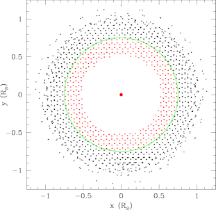
Figure 2.— Example of a star modeled with ghost particles (small red dots), SPH particles (black dots), which are found beyond the boundary (green line), and a central point mass (big red dot).

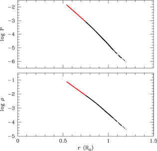
Figure 3.— Density and pressure profiles of the ghosts (red) and SPH particles (black) showing the gradients at the boundary, as expected for realistic models of stars. In all panels, only the particles located within $2h$ of the equatorial plane are plotted. The profiles of the ghost particles exactly match that of the theoretical profiles, showing that the overall profiles are very close the the theoretical ones.

4. Applications to binary stars

We now discuss the modeling of binary stars with our new boundary conditions. In particular, we develop a self-consistent technique for relaxing binary stars and show that our code, along with our new boundary conditions, can accurately follow and maintain two stars on relatively tight orbit for many tens of dynamical times. We emphasize that the location of the boundary is, at this point, arbitrary. We will discuss this issue in more details in $\S$4.3.

4.1. Binary star relaxation

As discussed in $\S$3.2.2, stars must be relaxed prior to being used in simulations. This is also true for binary systems since tidal effects are not taken into account when calculating the theoretical density profiles of the individual stars. Therefore, care must be taken when preparing binary systems for SPH simulations.

To account for the different hydrostatic equilibrium configuration of binary stars, we use the fact that the stars should be at rest in a reference frame that is centered at the centre of mass of the binary and that rotates with the same angular velocity as the stars. A centrifugal term is added to the acceleration of the SPH particles, which we find by requiring that it cancels the net gravitational acceleration of the stars (e.g. Rosswog et al. 2004; Gaburov et al. 2010). By assuming an initial orbital separation, we find, at each timestep, the necessary angular velocity $\Omega$ that cancels the stars’ net gravitational acceleration. Note that we do not account for the Coriolis force since the system is assumed to be at rest in the rotating frame. The net acceleration of the centre of mass of star $i$ is calculated in the following way:

$$\textbf{a}^{i}_{\textrm{cm}}=\frac{\sum m_{j}(\textbf{a}_{j}^{\textrm{hyd}}+\textbf{a}_{j}^{\textrm{grav}})}{M_{i}}$$ (7)

where $M_{i}$, $\textbf{a}_{hyd}$ and $\textbf{a}_{grav}$ are respectively the total mass and the hydrodynamical and gravitational accelerations of star $i$, and the summation is done over particles $j$ that are bound to star $i$. We therefore get the following condition for the angular velocity:

$$\Omega^{2}_{i}=\frac{\sum m_{j}(a_{j}^{\textrm{hyd}}+a_{j}^{\textrm{grav}})}{\sum m_{j}r_{j}}.$$ (8)

where $r_{j}$ is the distance of particle $j$ to the axis of rotation of the binary. We find the angular velocity for both stars and take the average value and add it to the acceleration of each SPH particle. To ensure that the orbital separation is kept constant during the relaxation, we also reset the stars to their initial positions after each timestep by a simple translation. An example of such a detached relaxed binary is shown in the left panel of Figure 4.

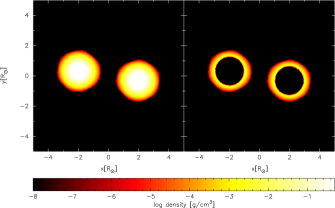
Figure 4.— Logarithm of density in the orbital plane for a detached relaxed binary with stars of $0.80$ M_⊙ fully modeled (left) and modeled with boundary conditions (right).

4.2. Circular orbits

After the initial relaxation, the stars are put in an inertial reference frame by using the value of the angular velocity obtained from the binary relaxation procedure. To assess the physicality and numerical integration capabilities of our hydrodynamical code, we have evolved different wide binaries on circular orbits for a small number of orbits. This is important for simulations of mass transfer as any changes in orbital separation must be driven by the mass transfer itself and not the initial conditions and/or numerical errors inherent to our method.

Figure 5 shows the normalized orbital separation and different energies as a function of time for a $0.60+0.60$ M_⊙ binary with each star fully modeled (i.e. without a boundary). Each star contains $\sim 105,000$ SPH particles and the initial separation is $3.25$ R_⊙. Our relaxation procedure yields an angular velocity of $\Omega=0.1875$ which, because of the large initial separation, is identical to the Keplerian value. The different forms of energy are all well conserved, as well as the orbital separation, which remains constant to better than $\sim 0.25\%$ for over six orbits. The slight (anti-symmetric) variations observed in the orbital separation and the kinetic energy are an indication that the system is on a slightly eccentric orbit. At this level, however, we estimate that our code can properly (and physically) evolve two stars orbiting around each other.

Figure 5.— Normalized energies and orbital separation as a function of time for a 0.6+0.6 M_⊙ circular binary modeled with $\sim$200,000 particles initially relaxed using the method of $\S$4.1 with fixed orbital separation.

Figure 6 shows the comparison between the normalized energies and orbital separation of a $0.80+0.80$ M_⊙ binary modeled with a different number of particles (the high resolution simulation is also shown in Figure 4). The solid and dotted lines correspond, respectively, to the systems modeled without and with boundary conditions. In the simulations shown here, the boundary is set at $75\%$ of the star’s radius. Figure 6 shows that introducing the boundary conditions smoothes the oscillations seen for the fully modeled binaries. This is explained by the fact that the calculation of the gravitational force on the central point mass, and hence most of the star’s mass, is done using a direct summation (instead of a binary tree), therefore improving the accuracy and reducing the oscillations in the orbital separation.

Figure 6.— Normalized total energy and orbital separation for a 0.80+0.80 M_⊙ circular binary modeled with (dotted line) and without (solid line) boundary conditions. The upper two panels are for a low-resolution simulation containing $\sim 40,000$ (full star) particles and the lower two panels are for a high-resolution simulation containing $\sim 240,000$ particles (full star).

Figure 6 also shows that increasing the spatial resolution increases the quality of the evolution of the orbits. For comparison, the orbital separation of our high-resolution simulation varies by less than $0.5\%$, compared to $\sim 2\%$ for the low-resolution (Figure 6). Moreover, in all cases, the total energy is conserved to $\sim 0.25\%$ over the whole duration of the simulations and the gravitational and thermal energies (not shown) remain constant to better than $\sim 0.5\%$.

Similarly, Figure 7 shows the evolution of a $0.80+0.48$ M_⊙ binary system over four orbits and a relatively low number of particles. Note that only the primary is modeled with the use of our boundary conditions for reasons that are discussed in $\S$6. Again, the orbital separation remains fairly close to its initial value, to within $2\%$ at the end of four orbits. The total energy is conserved to better than $0.5\%$ and only the kinetic energy oscillates significantly. We note that, when comparing our results of circular orbits with those of other authors, our binary relaxation procedure yields quantitatively comparable orbital behaviours. The results of Benz et al. (1990) show oscillations of $\sim 1-2\%$ in the orbital separation over three orbits whereas the simulations from Dan, Rosswog, & Brüggen (2008) of two unequal-mass binaries showed a constant orbital separation for many tens of orbits with an accuracy of $\sim 1\%$. Motl, Tohline, & Frank (2002) and D’Souza et al. (2006), using a specifically designed grid-based hydrodynamics code, both maintain equal- and unequal-mass binaries on circular orbits with an accuracy of $\sim 0.25\%$ over five orbits.

Figure 7.— Comparison of the normalized energies and orbital separation as a function of time for a 0.80+0.48 M_⊙ circular binary modeled with (dotted line) and without (solid line) boundary conditions.

Finally, we note that although our boundary condition treatment does require more calculations (e.g. the contribution from all the particles to the point mass’ acceleration), the simulations of binary systems can be sped up by up $\sim 50\%$ when modeled with boundary conditions. This depends of course on the location of the boundary, which at this point is arbitrary but chosen wherever it makes the most sense for the problem at hand. Note, however, that the boundary should be placed at least a few smoothing lengths from the surface of the star.

4.3. Eccentric Orbits

The case of an eccentric orbit is interesting since tidal forces are time-dependent and can vary greatly depending on the orbital phase. Here, we show that despite the large tidal forces at periastron, our boundary conditions are well suited for the modeling of such systems. The system we model consists of two main-sequence stars with masses of $1.40$ and $1.50$ M_⊙ with an eccentricity of $e=0.15$ and evolved for over four orbits ($P_{\textrm{orb}}\simeq 44$ code units). The total number of particles nears $\sim 500,000$ and the location of the boundary is at $\sim 75\%$ of the stars’ radius, which, as shown in Figure 8, is deep inside the star so that the effects of tidal force are negligible. Indeed, Figure 8 shows the radius of the primary enclosing different fractions of the total bound mass (in SPH particles) as a function of time for our binary system. For example, the radii containing $60\%$ to $90\%$ of the total bound mass are shown to not change significantly during the whole duration of this simulation. In fact, only the outer radius of the star, containing over $95\%$ of the bound mass, oscillates during each orbit. Therefore, in this case, the choice of the location of the boundary (dotted line) is well justified and Figure 8 shows that the use of our method for eccentric binaries is adequate. Replacing the core of a star with a central point mass and a boundary remains a valid approximation as long as the boundary is deep enough inside the envelope of the star.

Figure 8.— Radii enclosing different fractions of the total bound mass (in SPH particles) to the primary star as a function of time for the $1.40+1.50$ M_⊙ binary with $e=0.15$. The dotted line represents the location of the boundary.

5. Simulation of Mass Transfer

We now present the results from the simulation presented in $\S$4.3. In particular, we are interested in the mass transfer rates observed along the eccentric orbit. We also assess the physicality and limits of our approach later in $\S$6.

Figure 9 shows the logarithm of the density for particles close to the orbital plane. The use of our boundary conditions can be seen as the centre of the stars is devoid of particles, except for the central point masses (not shown). Short episodes of mass transfer are observed close to periastron while mass transfer stops as the stars get further apart. The material being transferred hits the secondary and disturbs its outer envelope such that the latter loses some material. In the end, the secondary is surrounded by a relatively thick envelope.

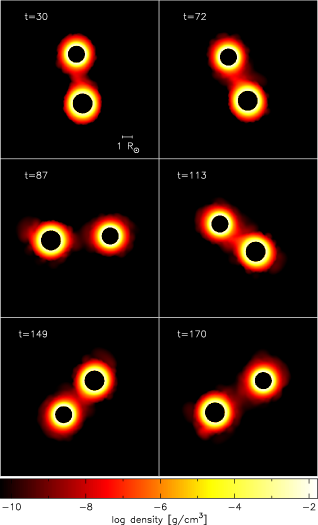
Figure 9.— Logarithm of the density in the orbital plane for the $1.40+1.50$ M_⊙ binary with $e=0.15$. The orbital period is about $44$ time units and the central point masses are not shown.

5.1. Determination of bound mass

To estimate the mass transfer rates, we have to determine the component to which every SPH particle is bound. We use a total-energy (per unit mass) criterion, as presented by Lombardi et al. (2006), and determine whether a particle is bound to the primary, the secondary, or the binary as a whole. In particular, given that most of the mass of the two stars is contained in the point masses, we use the latter as the main components to which particles are bound. For a particle to be bound to any of the components, we require its total energy relative to the component under consideration to be negative. The total energy of any particle with respect to both the point masses and the binary’s centre of mass is defined as

$$E_{ij}=\frac{1}{2}v_{ij}^{2}+u_{i}-\frac{G(M_{j}-m_{i})}{d_{ij}}$$ (9)

where $v_{ij}$ and $d_{ij}$ are the relative velocity and separation, respectively, between particle $i$ and component $j$. Moreover, we require the separation $d_{ij}$ to be less than the current separation of the two centres of mass of the stars (in this case, the point masses). For particles that satisfy both of these criteria for both stellar components, we assign them to the stellar component for which the total energy is most negative. If only the energy condition is satisfied for the stellar components, or the energy with respect to the binary is negative, the particle is assigned to the binary component. Finally, if the total relative energy is positive, the particle is unbound and is assigned to the ejecta.

5.2. Estimates of mass transfer rates

Using the total mass bound to the stellar components as a function of time, we can determine the mass transfer rates for the system modeled. We use a simple approach to determine the instantaneous mass transfer rates based on the difference of the total mass bound of each component between two successive timesteps, i.e.

$$\dot{M}=\frac{M^{i}_{t}-M^{i}_{t-1}}{\Delta t},$$ (10)

where $M$ refers to the bound mass and the indices refer to component $i$ and timesteps $t$ and $t-1$.

Figure 10 shows the mass transfer rate of the primary as a function of time. Distinct episodes of mass transfer are observed to occur once per orbit and peak around a few $10^{-6}$ M_⊙ yr^-1. The number of particles transferred during each episodes is $175-200$ which, given the masses of the SPH particles, may limit our ability to resolve lower mass transfer rates. Indeed, SPH requires a minimum number of neighbouring particles to calculate the density and in cases where only a handful of particles are transferred, the SPH treatment may not be adequate. Given the masses of the particles, low numbers of particles therefore set lower limits to the mass transfer rates that our simulations can resolve. Using more particles of smaller masses would definitely allow for the resolution of lower mass transfer rates, as discussed in $\S$6. Apart from the main episodes of mass transfer, we also observe secondary peaks occurring before the main episodes of mass transfer. Our simulation shows that some of the material lost both by the primary and the secondary falls back onto both components and this is what is observed here.

Figure 10.— Change in bound mass onto the primary as a function of time for the $1.40+1.50$ M_⊙ binary with $e=0.15$. The number of particles transferred during each episode is $\sim 200$, which represents an approximative lower limit to our ability to adequately resolve mass transfer due to the statistical nature of SPH.

6. Discussion

Analytical approaches used to study the evolution of binaries usually rely on prescriptions or approximations when dealing with mass transfer rates. To relax some of these approximations, hydrodynamical modeling can be used, although it remains a hard task for many physical and numerical reasons. To circumvent some of these difficulties, we introduced an alternate technique using boundary conditions and ghost particles to model only the outermost parts of both the donor and the accretor stars. The location of the boundary is arbitrarily set. Since only the surface material is involved in mass transfer, our approach allows for better spatial and mass resolutions in the stream of matter. Moreover, our method allows for the modeling of both the accretor and the donor simultaneously while using less CPU time and maintaining realistic density profiles, taken from stellar models.

Our code was shown to work particularly well for stars of equal mass and stars that are centrally condensed. Indeed, replacing the dense core of a massive star by a point mass is a good approximation. This is generally true for stars with masses $\gtrsim 0.8$ M_⊙, although the evolutionary stage of the star may modify its density profile. Low-mass stars have shown to be more difficult to properly model with our approach (see Figure 7) and we suggest that limiting our new boundary conditions to centrally condensed stars will in general yield better results.

We also discussed the setup of proper initial conditions for modeling binary stars, which we have tested on both equal- and unequal-mass binaries. We demonstrated that our relaxation procedure is consistently implemented in our code and that it allows for the evolution over many orbits of equal-mass detached circular binaries and maintain their orbital separation to within $1-2\%$.

In light of the results from our first simulation of mass transfer, we establish that typical mass transfer rates that can be modeled with our new boundary conditions (i.e. $\gtrsim 10^{-6}$ M_⊙ yr^-1) are consistent with the estimates of Chen & Han (2008) who investigated the formation of blue stragglers through episodes of mass transfer onto main-sequence stars. We therefore suggest that our method consisting of modeling both stars simultaneously with appropriate boundary conditions can be applied to the problem of mass transfer in main-sequence binaries and help clarify the origin of blue stragglers.

Using particles of lower mass allows for the modeling of lower mass transfer rates, although this requires the use of more particles and CPU time. Pushing the boundary further out or using a point mass to model the secondary (as in Church et al. 2009) can also allow for the use of more particles and a better mass transfer rate resolution. Using a point mass as the secondary would however counter the benefit of our method to be able to model two interacting stars simultaneously.

The physicality of our simulations depends of course on the physical ingredients we put in our code. As such, we do not include the effects of radiation pressure and energy transport mechanisms by radiation or convection. These effects may have significance especially when studying the long-term evolution of mass-transferring binaries, where radiative cooling in the outer layers of the stars and envelope might be more important. Moreover, like any numerical technique, our method has some of its own limitations, and we discuss them now.

6.1. Solid boundary

By construction, our boundary is “semi-impermeable”, in that it does not allow particles to go through it. We set three smoothing lengths of ghosts and enforce that particles be artificially repositioned if they happen to cross the boundary. However, it is possible that these conditions fail when dealing with large mass transfer rates and if some particles find themselves inside the boundary, around the central point mass, our code has to be stopped. This particle penetration limits our ability to adequately model episodes of extremely (and unrealistically) large mass transfer rates ($\gtrsim 10^{-1}$ M_⊙ yr^-1; see Paper II). However, we do not think that our boundary should be so particle-tight since we do expect some mixing in the envelope of the secondaries. Although moving the boundary to a smaller radius could fix the issue of particle penetration, it would counter the use and benefits of our approach. Instead, we suggest using sink particles at the centre of the stars in order to account for deep mixing. Sink particles are like point masses but, in addition, their mass and momentum are allowed to increase as SPH particles get accreted.

Also, as discussed in $\S$3.2, the relative position of our ghost particles is fixed in time, thus imitating a solid boundary. The boundary is not allowed to change its shape and/or provide a time-variable pressure gradient on the SPH particles. As a first approximation, this is a valid treatment (e.g. Deupree & Karakas 2005). However, when the gravitational potential changes significantly along the orbit, like on eccentric orbits, tidal forces may become non-negligible. But modeling the effect of tidal forces on the boundary is costly, in terms of CPU time, as it involves calculating the gravitational force on the ghosts. This calculation is not done in our code as of now. We showed, however, that placing the boundary deep inside the star decreases the effect of tidal forces on the boundary and validates the use of our method. Finally, we note that the angular velocity of the ghost particles is maintained fixed during our simulations. This is a valid assumption as synchronization occurs over timescales that are much longer ($10^{6}-10^{8}$ years) than the duration of our simulations.

6.2. Relaxation of unequal-mass binaries

Our relaxation procedure for binary stars has proven to be especially efficient for equal-mass binaries. However, for unequal-mass binaries, we do not quite achieve the same level of accuracy for the evolution of orbital separation. We think the reason for this difference comes from the fact that the equal-mass systems we model are perfectly symmetric, i.e. the two stars are exact replicas of each other, whereas in the case of unequal-mass binaries, symmetry is broken. For equal-mass binaries, the gravitational acceleration calculations are exactly equal and opposite and the two stars are evolved identically. But given the adaptive nature of our code, stars (and particles) of different masses may be evolved on different timesteps and care should be taken if the two stars (and particles) are to be evolved consistently. We performed test runs during which we forced our code to use a smaller common timestep, but this approach does not improve the results. On the other hand, using a more direct summation approach for the calculation of the gravitational force (by using a smaller binary tree opening angle) is found to improve the results. Indeed, results from test runs using such an approach show much improvements in evolving stars on circular orbits. However, doing so also makes our simulations significantly longer to run. Therefore, we think the observed behaviour of our unequal-mass binaries is the result of our calculation of gravitational acceleration through a binary tree, although more work remains to be done.

6.3. Future Work

The method presented in this paper has been shown to be well suited for modeling the hydrodynamics of interacting binary stars. Here, we used it to model Roche lobe overflow, during which only the outermost layers of the stars are actively involved. We propose that the approach presented in this work can also be applied to many different situations, such as wind accretion and interstellar medium accretion, and that it can help better understand how stars react to mass loss and mass accretion in general. In particular, we have emphasized that the Roche lobe formalism is not applicable in the case of eccentric and asynchronous binaries. We think our alternate method can be used to better understand and characterize the onset of mass transfer in such systems. This is the subject of a subsequent paper (Lajoie & Sills, 2010) in which we model eccentric systems of different masses, semi-major axes, and eccentricities.

References

- Abt & Levy (1976) Abt, H.A & Levy, S.G. 1976, ApJS, 30, 273
- Bate et al. (1995) Bate, M.R., Bonnell, I.A., & Price, N.M. 1995, MNRAS, 277, 362
- Bate (1995) Bate, M.R. 1995, Ph.D. Thesis, University of Cambridge, UK
- Benz (1990) Benz, W. 1990, in Buchler J.R., ed. The Numerical Modeling of Nonlinear Stellar Pulsations: Problems and Prospects. Kluwer, Dordrecht, p.26 9
- Benz et al. (1990) Benz, W., Bowers, R.L., Cameron, A.G.W., & Press, W. 1990, ApJ, 348, 647
- Bisikalo et al. (1998) Bisikalo, D.V. et al. 1998, MNRAS, 300, 39
- Blondin et al. (1995) Blondin, J.M., Richards, M.T., & Malinowski, M.L. 1995, ApJ, 445, 939
- Chen & Han (2008) Chen, X., & Han, Z. 2008, MNRAS, 387, 1416
- Church et al. (2009) Church, R.P., Dischler, J., Davies, M.B., Tout, C.A., Adams, T., & Beer, M.E. 2009, MNRAS, 395, 1127
- Crawford (1955) Crawford, J.A. 1955, ApJ, 121, 71
- Cummins & Rudman (1999) Cummins, S.J, & Rudman, M. 1999, \jocp, 152, 584
- D’Souza et al. (2006) D’Souza, M.C.R., Motl, P.M., Tohline, J.E., & Frank, J. 2006, ApJ, 643, 381
- Dan, Rosswog, & Brüggen (2008) Dan, M. Rosswog, S., & Brüggen, M. 2008, arXiv:0811.1517
- Dermine et al. (2009) Dermine, T., Jorissen, A., Siess, L., & Frankowski, A. 2009, A&A, 507, 891
- Deupree & Karakas (2005) Deupree, R.G., & Karakas, A.I. 2005, ApJ, 633, 418
- Duquennoy & Mayor (1991) Duquennoy, A. & Mayor, M. 1991, å, 248, 485
- Eggleton (1983) Eggleton, P.P. 1983, ApJ, 268, 368
- Eggleton (2006) Eggleton, P.P. 2006, Evolutionary Processes in Binary and Multiple Stars. Cambridge Univ. Press, Cambridge
- Fischer & Marcy (1992) Fischer, D.A. & Marcy, G.W. 1992, ApJ, 396, 178
- Flannery (1975) Flannery, B.P. 1975, ApJ, 201, 661
- Gaburov et al. (2010) Gaburov, E., Lombardi, J.C. Jr, & Portegies Zwart, S. 2010, MNRAS, 402, 105
- Gingold & Monaghan (1977) Gingold, R.A., & Monaghan, J.J. 1977, MNRAS, 181, 375
- Gokhale et al. (2007) Gokhale, V., Peng, X.M., & Frank, J. 2007, ApJ, 655, 1010
- Governato et al. (2009) Governato, F. et al. 2009, MNRAS, 398, 312
- Guenther et al. (1992) Guenther, D.B., Demarque, P., Kim, Y.-C., & Pinsonneault, M.H. 1992, ApJ, 387, 372
- Halbwachs et al. (2003) Halbwachs, J.L., Mayor, M., Udry, S., & Arenou, F. 2003, A&A, 397, 159
- Iben (1991) Iben, I. Jr 1991, ApJS, 76, 55
- Lajoie & Sills (2010) Lajoie, C.-P., & Sills, A. 2010, ApJ, submitted
- Lombardi et al. (1995) Lombardi, J.C. Jr., Rasio, F.A., & Shapiro, S.L. 1995, ApJ, 445, L117
- Lombardi et al. (1999) Lombardi, J.C. Jr., Sills, A., Rasio, F.A., & Shapiro, S.L. 1999, \jocp, 152, 687
- Lombardi et al. (2006) Lombardi, J.C. Jr., Proulx, X.F., Dooley, K.L., Theriault, E.M., Ivanova, N., & Rasio, F.A. 2006, ApJ, 640, 441
- Lubow & Shu (1975) Lubow, S. H., & Shu, F. H. 1975, ApJ, 198, 383
- Lucy (1977) Lucy, L.B. 1977, AJ, 82, 1013
- Mashchenko, Couchman, & Wadsley (2006) Mashchenko, S., Couchman, H.M.P., & Wadsley, J. 2006, Nature, 442, 539
- Mayer et al. (2007) Mayer, L. et al. 2007, ApJ, 661, L77
- Monaghan & Lattanzio (1985) Monaghan, J.J. & Lattanzio, J.C. 1985, A&A, 149, 135
- Monaghan (1989) Monaghan, J.J. 1989, \jocp, 82, 1
- Monaghan (1994) Monaghan, J.J. 1994, \jocp, 110, 399
- Morris, Fox, & Zhu (1997) Morris, J.P., Fox, P.J., & Zhu, Y. 1997, \jocp, 136, 214
- Morton (1960) Morton, D.C. 1960, ApJ, 132, 146
- Motl, Tohline, & Frank (2002) Motl, P.M., Tohline, J.E., & Frank, J. 2002, ApJS, 138, 121
- Paczyński (1965) Paczyński, B. 1965, Acta Astron., 15, 89
- Paczyński (1971) Paczyński, B. 1971, ARA&A, 9, 183
- Paczyński & Sienkiewicz (1972) Paczyński, B., & Sienkiewicz, R. 1972, Acta Astron., 22, 73
- Petrova & Orlov (1999) Petrova, A.V., & Orlov, V.V. 1999, AJ, 117, 587
- Pooley & Hut (2006) Pooley, D., & Hut, P. 2006, ApJ, 646, L143
- Price (2005) Price, D. 2005, PhD thesis, Univ. Cambridge (astro-ph/0507472)
- Price & Bate (2009) Price, D., & Bate, M.R. 2009, MNRAS, 398, 33
- Raguzova & Popov (2005) Raguzova, N.V. & Popov, S.B. 2005, Astron. Astrophys. Trans., 24, 151
- Rasio & Shapiro (1994) Rasio, F.A., & Shapiro, S.L. 1994, ApJ, 432, 242
- Rasio & Shapiro (1995) Rasio, F.A., & Shapiro, S.L. 1995, ApJ, 438, 887
- Ritter (1988) Ritter, H. 1988, A&A, 202, 93
- Rodono (1992) Rodono, M. 1992, in Kondo, Sistero, & Polidan, eds, IAU Symp. 151, Evolutionary Processes in Interacting Binary Stars, Kluwer-Dordrecht, p.71
- Rosswog et al. (2004) Rosswog, S., Speith, R., & Wynn, G.A. 2004, MNRAS, 351, 1121
- Sawada et al. (1986) Sawada, K., Matsuda, T.,& Hachisu, I. 1986, MNRAS, 219, 75
- Sepinsky et al. (2007a) Sepinsky, J.F., Willems, B., & Kalogera, V. 2007a, ApJ, 660, 1624
- Sepinsky et al. (2007b) Sepinsky, J.F., Willems, B., Kalogera, V., & Rasio, F.A. 2007b, ApJ, 667, 1170
- Sepinsky et al. (2009) Sepinsky, J.F., Willems, B., Kalogera, V., & Rasio, F.A. 2009, ApJ, 702, 1387
- Sills & Lombardi (1997) Sills, A.I., & Lombardi, J.C.Jr 1997, ApJ, 484, L51
- Sills et al. (1997) Sills, A., Lombardi Jr., J.C., Bailyn, C.D., Demarque, P., Rasio, F.A., & Shapiro, S.L. 1997, ApJ, 487, 290
- Sills et al. (2001) Sills, Faber, J.A., Lombardi Jr., J.C., Rasio, F.A., & Warren, A.R. 2001, ApJ, 548, 323
- Stinson et al. (2009) Stinson, G.S. et al. 2009, MNRAS, 395, 1455
- Takeda, Miyama, & Sekiya (1994) Takeda, H., Miyama, S. M., & Sekiya, M. 1994, Prog. Theo. Phys., 92, 939
- Tohline (2002) Tohline, J.E. 2002, ARA&A, 40, 349
- Warner & Peters (1972) Warner, B., & Peters, W.L. 1972, MNRAS, 160, 15