Monte Carlo simulations of the Nickel K$\alpha$ fluorescent emission line in a toroidal geometry

Abstract

We present new results from Monte Carlo calculations of the flux and equivalent width (EW) of the Ni K$\alpha$ fluorescent emission line in the toroidal X-ray reprocessor model of Murphy & Yaqoob (2009, MNRAS, 397, 1549). In the Compton-thin regime, the EW of the Ni K$\alpha$ line is a factor of $\sim 22$ less than that of the Fe K$\alpha$ line but this factor can be as low as $\sim 6$ in the Compton-thick regime. We show that the optically-thin limit for this ratio depends only on the Fe to Ni abundance ratio, it being independent of the geometry and covering factor of the reprocessor, and also independent of the shape of the incident X-ray continuum. We give some useful analytic expressions for the absolute flux and the EW of the Ni K$\alpha$ line in the optically-thin limit. When the reprocessor is Compton-thick and the incident continuum is a power-law with a photon index of 1.9, the Ni K$\alpha$ EW has a maximum value of $\sim 3$ eV and $\sim 250$ eV for non-intercepting and intercepting lines-of-sight respectively. Larger EWs are obtained for flatter continua. We have also studied the Compton shoulder of the Ni K$\alpha$ line and find that the ratio of scattered to unscattered flux in the line has a maximum value of 0.26, less than the corresponding maximum for the Fe K$\alpha$ line. However, we find that the shape of the Compton shoulder profile for a given column density and inclination angle of the torus is similar to the corresponding profile for the Fe K$\alpha$ line. Our results will be useful for interpreting X-ray spectra of active galactic nuclei (AGNs) and X-ray binary systems in which the system parameters are favorable for the Ni K$\alpha$ line to be detected.

Keywords: galaxies: active - line:formation - radiation mechanism: general - scattering - X-rays: general

1 Introduction

The Ni K$\alpha$ fluorescent emission line has the potential to offer complementary diagnostics to the Fe K$\alpha$ fluorescent line in active galactic nuclei (AGNs) and some X-ray binary systems in which the Fe K$\alpha$ line is detected (e.g., see Torrejón et al. 2010, and references therein). In AGNs, the narrow Fe K$\alpha$ emission line is a ubiquitous feature of the X-ray spectrum of both type 1 and type 2 sources (e.g. see Shu, Yaqoob, & Wang 2010, and references therein). However, since the abundance of Ni is more than an order of magnitude less than that of Fe, the Ni K$\alpha$ line is expected to be weak. Nevertheless, it has been detected in a few AGNs. Three of the best examples are the Circinus galaxy (Molendi, Bianchi, & Matt 2003), NGC 6552 (Reynolds et al. 1994), and NGC 1068 (Matt et al. 2004; Pounds & Vaughan 2006). In all of these sources the equivalent width of the Fe K$\alpha$ line is large (hundreds of eV, to over 1 keV) because the X-ray spectrum is dominated by, or has a relatively large contribution from, reflection in Compton-thick matter. Naturally, such sources are the most likely to yield detections of the Ni K$\alpha$ line because its EW will also be correspondingly larger, in tandem with that of the Fe K$\alpha$ line EW. The Ni K$\alpha$ line has also been detected in a source that is not reflection-dominated, but still moderately absorbed (Centaurus A), albeit with a lower statistical significance of detection (Markowitz et al. 2007). Improvements in the sensitivity of X-ray detectors in the $\sim 7-10$ keV band aboard forthcoming X-ray astronomy missions such as NuStar and Astro-H will likely reveal detections of the Ni K$\alpha$ emission line in a larger number of accreting X-ray sources and will therefore open up the opportunity to use the line as a diagnostic tool in conjunction with the Fe K$\alpha$ line.

The results of model calculations of the flux and EW of a Ni K$\alpha$ fluorescent line that originates in neutral matter, as expected in AGNs, have been reported in the literature for disk and spherical geometries (e.g., Reynolds et al. 1994; Matt, Fabian, & Reynolds 1997). In the present paper we study the theoretical properties of the Ni K$\alpha$ line produced by the toroidal X-ray reprocessor model of Murphy & Yaqoob (2009; hereafter, MY09). The paper is organized as follows. In §2 we give a brief overview of the model and key assumptions. We present the results of Monte Carlo simulations for the Ni K$\alpha$ line flux and EW in §3 and §4 respectively. In §5 we show results for the ratio of the Compton-scattered to unscattered line flux and we discuss the Compton shoulder of the Ni K$\alpha$ emission line. We summarize our conclusions in §6.

2 Toroidal X-ray reprocessor model overview

Here we give a brief overview of our model Monte Carlo simulations and the key assumptions that they are based upon (further details can be found in MY09). We assume that the reprocessing material is uniform and neutral (cold). X-ray spectroscopy of AGNs shows overwhelming evidence for the narrow Fe K$\alpha$ line peaking at $\sim 6.4$ keV, indicating that the matter responsible for producing that line is essentially neutral (e.g. Sulentic et al. 1998; Weaver, Gelbord, & Yaqoob 2001; Page et al. 2004; Yaqoob & Padmanabhan 2004; Jiménez-Bailón et al. 2005; Zhou & Wang 2005; Jiang, Wang, & Wang 2006; Levenson et al. 2006; Shu et al. 2010). Although emission lines from ionized species of Fe are observed in some AGN (e.g. Yaqoob et al. 2003; Bianchi et al. 2005, 2008), the present paper is concerned specifically with modeling the Ni K$\alpha$ fluorescent emission line that originates in the same material as the Fe K$\alpha$ line component that is centered around 6.4 keV. We note that this Fe K$\alpha$ line at $\sim 6.4$ keV is also observed in some X-ray binaries (e.g., Torrejón et al. 2010) but it is not as common as it is in AGNs.

Our geometry is an azimuthally-symmetric doughnut-like torus with a circular cross-section, characterized by only two parameters, namely the half-opening angle, $\theta_{0}$, and the equatorial column density, $N_{\rm H}$ (see Fig. 1 in MY09). If $a$ is the radius of the circular cross-section of the torus, and $c+a$ is the equatorial (i.e. maximum) radius of the torus then $(a/c)$ is a covering factor such that $(a/c)=[\Delta\Omega/(4\pi)]$. Here, $\Delta\Omega$ is the solid angle subtended by the torus at the X-ray source, which is assumed to be located at the center of the system, emitting isotropically. The mean column density, integrated over all incident angles of rays through the torus, is then $\bar{N}_{\rm H}$ $=(\pi/4)$$N_{\rm H}$. The inclination angle between the observer’s line of sight and the symmetry axis of the torus is denoted by $\theta_{\rm obs}$, where $\theta_{\rm obs}$ $=0^{\circ}$ corresponds to a face-on observing angle and $\theta_{\rm obs}$ $=90^{\circ}$ corresponds to an edge-on observing angle. In our calculations we distribute the emergent photons in 10 angle bins between $0^{\circ}$ and $90^{\circ}$ that have equal widths in $\cos{\theta_{\rm obs}}$, and refer to the face-on bin as #1, and the edge-on bin as #10 (see Table 1 in MY09).

The value of $\theta_{0}$ for which we have calculated a comprehensive set of models is $60^{\circ}$, for $N_{\rm H}$ in the range $10^{22}\ \rm cm^{-2}$ to $10^{25}\ \rm cm^{-2}$, valid for input spectra with energies in the range 0.5–500 keV (see MY09 for details). Our model employs a full relativistic treatment of Compton scattering, using the full differential and total Klein-Nishina Compton-scattering cross-sections. For $\theta_{0}=60^{\circ}$, the solid angle subtended by the torus at the X-ray source, $\Delta\Omega$, is $2\pi$, so that $[\Delta\Omega/(4\pi)]=(a/c)=0.5$.

We utilized photoelectric absorption cross-sections for 30 elements as described in Verner & Yakovlev (1995) and Verner et al. (1996) and we used Anders and Grevesse (1989) elemental cosmic abundances in our calculations. The Thomson depth may also be expressed in terms of the column density: $\tau_{\rm T}=KN_{\rm H}\sigma_{\rm T}\sim 0.809N_{24}$ where $N_{24}$ is the column density in units of $10^{24}\rm\ cm^{-2}$. Here, we have employed the mean number of electrons per H atom, $\frac{1}{2}(1+\mu)$, where $\mu$ is the mean molecular weight. With the abundances of Anders & Grevesse, $K=1.21656$, assuming that the number of electrons from all other elements aside from H and He is negligible. The Anders & Grevesse (1989) value for the solar Ni abundance, $A_{\rm Ni}$, is $1.78\times 10^{-6}$ relative to H. A more recent determination by Scott et al. (2009) yields a value of $1.48\times 10^{-6}$ but the statistical and systematic uncertainties do not exclude the Anders & Grevesse (1989) value. We use the latter for consistency with our previous results on the Fe K$\alpha$ emission line (MY09; Yaqoob et al. 2010; Yaqoob & Murphy 2010).

The Ni K$\alpha$ fluorescent emission line consists of two components, $K\alpha_{1}$ and $K\alpha_{2}$, at energies $7.4782$ keV and $7.4609$ keV respectively, and with a branching ratio of $K\alpha_{1}:K\alpha_{2}=2:1$ (Bearden 1967). These line energies are appropriate for neutral matter. In the Monte Carlo simulations we used a single line for Ni K$\alpha$, at a rest-frame monoenergetic energy, $E_{0}$, of 7.472 keV (obtained from weighting the $K\alpha_{1}$ and $K\alpha_{2}$ values with the branching ratio). We used a fluorescence yield, $\omega_{K}$, for Ni of 0.414 (see Bambynek et al. 1972) and a Ni K$\beta$ to Ni K$\alpha$ ratio of 0.135 (consistent with results in Bambynek et al. 1972).

Compared to MY09, the results in the present paper have a substantially higher statistical accuracy because they are based on Monte Carlo simulations with higher numbers of injected rays at each energy, and the calculations employ the method of weights (as opposed to following individual photons). Throughout the present paper we present results for power-law incident continua (in the range 0.5–500 keV), characterized by a photon index, $\Gamma$, by integrating the basic monoenergetic Monte Carlo results (Greens functions– see MY09).

3 Ni K$\alpha$ line flux

In this section we discuss the flux of Ni K$\alpha$ emission-line photons that escape the torus without any interaction with it (the zeroth-order, or unscattered line photons). In §5 we will discuss the scattered component of the line emission (the Compton shoulder). In practice it may not actually be possible to observationally distinguish the zeroth-order component of an emission line from its Compton shoulder. The finite energy resolution of the instrument and/or the velocity broadening (of all the emission-line components) may confuse the two blended components of a line (see discussion in Yaqoob & Murphy 2010 for the Fe K$\alpha$ line). The Monte Carlo results for the flux of the zeroth-order component of the Ni K$\alpha$ emission line are shown in Fig. 1 as a function of the equatorial column density, $N_{\rm H}$, for each of the 10 angle bins in $\theta_{\rm obs}$. The line flux, $I_{\rm Ni\ K\alpha}$, has been normalized to an incident continuum that has a monochromatic flux of 1 photon $\rm cm^{-2}\ s^{-1}\ keV^{-1}$ at 1 keV.

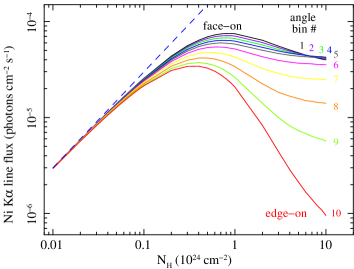
Figure 1: The Ni K$\alpha$ line flux versus $N_{\rm H}$ for $\Gamma=1.9$. Curves are shown for each of the 10 $\theta_{\rm obs}$ bins and are color coded and labeled by the angle bin number (see Table 1 in MY09). The angle bins correspond to equal solid angle intervals in the range $0^{\circ}$ to $90^{\circ}$. Angle bins 1–5 correspond to lines-of-sight that do not intercept the torus and angle bins 6–10 correspond to lines-of-sight that intercept the torus. The normalization of the line flux corresponds to a power-law incident continuum that has a monochromatic flux at 1 keV of $1\rm\ photons\ cm^{-2}\ s^{-1}\ keV^{-1}$. The dashed line corresponds to the optically-thin limit for the relation between the Ni K$\alpha$ line flux and $N_{\rm H}$ (equation 1).

As $N_{\rm H}$ is increased, the Ni K$\alpha$ line flux first increases but then turns over, reaching a maximum for $N_{\rm H}$ somewhere in the range $\sim 3-8\times 10^{23}\ \rm cm^{-2}$, depending on the inclination angle. This is because the escape of Ni K$\alpha$ line photons from the medium after they are created is significantly impeded by the absorption and scattering opacity that is relevant at the line energy. For the edge-on angle bin the maximum Ni K$\alpha$ line flux is attained well before the medium becomes Compton-thick, at only $\sim 3\times 10^{23}\ \rm cm^{-2}$. For the face-on angle bin the maximum line flux is attained at a higher column density ($\sim 8\times 10^{23}\ \rm cm^{-2}$), but still before the medium becomes Compton-thick. The position of the turnover can be understood as approximately corresponding to a situation when the average optical depth to absorption plus scattering for the zeroth-order Ni K$\alpha$ line photons is of order unity. The behavior of the Ni K$\alpha$ zeroth-order line flux as a function of $N_{\rm H}$ and $\theta_{\rm obs}$ is in fact very similar to that of the flux of the Fe K$\alpha$ line, for which a detailed discussion can be found in Yaqoob et al. (2010).

3.1 Ni K$\alpha$ line flux in the optically-thin limit

In the optically-thin limit, for which absorption and scattering optical depths in the $\sim 7-9$ keV band are $\ll 1$, we can obtain an approximate analytic expression for the Ni K$\alpha$ line flux. Following Yaqoob et al. (2001), we get

$$I_{\rm Ni\ K\alpha} \sim 8.647\times 10^{-4}\ \left(\frac{\Delta\Omega}{4\pi}\right)\ \left(\frac{\omega_{K}}{0.414}\right)\ \left(\frac{\omega_{K\alpha}}{\omega_{K}}\right)$$ (1)

$$\times \ \left(\frac{\rm A_{\rm Ni}}{1.78\times 10^{-6}}\right)\ \left(\frac{\sigma_{0}}{2.86\times 10^{-20}\rm\ cm^{2}}\right)$$

$$\times \ \left(\frac{3.61}{\Gamma+\alpha-1}\right)\ \left(8.348\ {\rm keV}\right)^{(1.9-\Gamma)}\ \ \ \bar{N}_{24}$$

$${\rm photons\ cm^{-2}\ s^{-1}}$$

The quantity $[\Delta\Omega/(4\pi)]$ is the fractional solid angle that the line-emitting matter subtends at the X-ray source. Note that equation 1 utilizes the mean (angle-averaged) column density, not the equatorial column density. Thus, $\bar{N}_{24}=(\pi/4)[N_{\rm H}/(10^{24}\ \rm cm^{-2})]$. The K-shell fluorescence yield is given by $\omega_{K}$, and $\omega_{K\alpha}$ is the yield for the Ni K$\alpha$ line only. Using our adopted value of 0.135 for the Ni K$\beta$/Ni K$\alpha$ line ratio, $\omega_{K\alpha}/\omega_{K}=0.881$. The quantity $A_{\rm Ni}$ is the Ni abundance relative to Hydrogen ($1.78\times 10^{-6}$, Anders & Grevesse 1989). The quantity $\sigma_{0}$ is the Ni K shell absorption cross-section at the Ni K photoelectric absorption edge threshold energy, $E_{K}$, and $\alpha$ is the power-law index of the cross-section as a function of energy. For the Verner et al. (1996) data that we have adopted, $E_{K}=8.348$ keV, $\sigma_{0}=2.68\times 10^{-20}\ \rm cm^{2}$, and $\alpha=2.71$ (obtained from fitting the K-shell cross-section up to 30 keV with a power-law model).

The optically-thin limit for the Ni K$\alpha$ line flux from equation 1 is shown in Fig. 1 (dashed line). It can be seen that the Monte Carlo curves converge to this optically-thin limit, but only for column densities $<2\times 10^{22}\ \rm cm^{-2}$. Note that the optically-thin limit for the Ni K$\alpha$ line flux is independent of the details of the geometry.

We can obtain a simple result in the optically-thin limit from equation 1 for the ratio of the Fe K$\alpha$ to Ni K$\alpha$ line flux. Neglecting the small difference in the energy dependence of the K-shell cross-section in Ni and Fe ($\sim E^{-2.71}$ and $\sim E^{-2.67}$ respectively), we have

$$\frac{I_{\rm Fe\ K\alpha}}{I_{\rm Ni\ K\alpha}} \sim 30.0\left(\frac{7.124\rm\ keV}{8.348\ \rm keV}\right)^{(1.9-\Gamma)}\frac{[A_{\rm Fe}/A_{\rm Ni}]}{[A_{\rm Fe}/A_{\rm Ni}]_{\rm AG89}}\ .$$ (2)

In equation 2, 7.124 keV is the neutral Fe K shell threshold edge energy in Verner et al. (1996), $[A_{\rm Fe}/A_{\rm Ni}]_{\rm AG89}$ is the Anders & Grevesse (1989) Fe to Ni abundance ratio (26.3), and $[A_{\rm Fe}/A_{\rm Ni}]$ is the actual Fe to Ni abundance ratio in the source. What is interesting about equation 2 is that not only is it independent of geometry, it is independent of the covering factor.

4 The Ni K$\alpha$ line equivalent width

In Fig. 2, we show the EWs of the unscattered (zeroth-order) component of the Ni K$\alpha$ line as a function of the column density of the torus, $N_{\rm H}$, calculated for $\Gamma=1.9$. The lower set of curves show the results for the non-intercepting angle bins, and the upper set of curves show the results for the intercepting angle bins, as indicated by the color-coded angle bin numbers. It can be seen in Fig. 2 that inclination-angle effects become important for $N_{\rm H}$ greater than $\sim 5\times 10^{22}\ \rm cm^{-2}$. For inclination angles that do not intercept the torus, the EW peaks between $\sim 8\times 10^{23}\rm\ cm^{-2}\ and\ 10^{24}\ cm^{-2}$, then decreases by more than $50$% of this peak value at $N_{\rm H}$ $=10^{25}\ \rm cm^{-2}$. For these non-intercepting lines-of-sight, the peak value for the EW of the Ni K$\alpha$ line, for $\Gamma=1.9$, is $\sim 3$ eV. For the lines-of-sight that intercept the torus, the Ni K$\alpha$ line EW reaches its maximum value between $N_{\rm H}\sim 2-4\times 10^{24}\ \rm cm^{-2}$, becoming as high as $\sim 250$ eV for the edge-on angle bin. Overall, the behavior of the EW as a function of $N_{\rm H}$ and $\theta_{\rm obs}$ is analogous to that of the Fe K$\alpha$ line, for which a detailed discussion can be found in MY09.

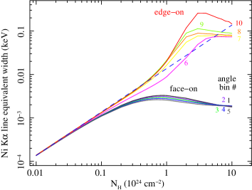
Figure 2: The Ni K$\alpha$ line equivalent width (EW) versus $N_{\rm H}$ for $\Gamma=1.9$. Curves are shown for each of the 10 $\theta_{\rm obs}$ bins and are color coded with the same scheme as in Fig. 1, and labeled by the angle bin number (see Table 1 in MY09). The angle bins correspond to equal solid angle intervals in the range $0^{\circ}$ to $90^{\circ}$. Angle bins 1–5 correspond to lines-of-sight that do not intercept the torus and angle bins 6–10 correspond to lines-of-sight that intercept the torus. The dashed line corresponds to the optically-thin limit for the relation between the Ni K$\alpha$ line EW and $N_{\rm H}$ (equation 3).

4.1 Ni K$\alpha$ line EW in the optically-thin limit

Overlaid on the curves in Fig. 2 is the theoretical optically-thin limit (dashed line), given by dividing equation 1 by $E^{-\Gamma}$ (recall that the line flux in equation 1 is normalized to a power-law continuum normalization at 1 keV of 1 $\rm photon\ cm^{-2}\ s^{-1}\ keV^{-1}$). Thus, the EW of the Ni K$\alpha$ line in the optically-thin limit is

$$EW_{\rm Ni\ K\alpha} \sim 39.48\ \left(\frac{\Delta\Omega}{4\pi}\right)\ \left(\frac{\omega_{K}}{0.414}\right)\ \left(\frac{\omega_{K\alpha}}{\omega_{K}}\right)$$ (3)

$$\times \left(\frac{\rm A_{\rm Fe}}{1.78\times 10^{-6}}\right)\ \left(\frac{\sigma_{0}}{2.86\times 10^{-20}\rm\ cm^{2}}\right)$$

$$\times \left(\frac{3.61}{\Gamma+\alpha-1}\right)\ \left(\frac{E_{0}}{E_{K}}\right)^{(\Gamma-1.9)}\ \bar{N}_{24}\ \ \ \rm eV\ .$$

As in equation 1, the column density in equation 3 is the mean, angle-averaged column density ($\bar{N}_{24}=(\pi/4)[N_{\rm H}/(10^{24}\ \rm cm^{-2})]$). In equation 3 $E_{0}$ is the Ni K$\alpha$ line centroid energy. The ratio $(E_{0}/E_{K})$ is $(7.472/8.348)=0.895065$. This happens to be very similar to the corresponding ratio for the Fe K$\alpha$ line, $(6.400/7.124)=0.898372$. This leads to a very simple expression for the approximate ratio between the EW of the Fe K$\alpha$ line and the EW of the Ni K$\alpha$ line in the optically-thin limit, that is independent of the shape of the intrinsic continuum. In analogy to equation 2, we get

$$\frac{EW_{\rm Fe\ K\alpha}}{EW_{\rm Ni\ K\alpha}} \sim 22.2\frac{[A_{\rm Ni}/A_{\rm Fe}]}{[A_{\rm Ni}/A_{\rm Fe}]_{\rm AG89}}\ .$$ (4)

As was the case for the line flux ratio, the EW ratio in the optically-thin limit is independent of geometry and the covering factor. Note that in the Compton-thick regime, for lines-of-sight that intercept the torus, the Ni K$\alpha$ line EW is larger relative to the Fe K$\alpha$ line EW than simple linear scaling of the optically-thin case. In other words, the EW ratio in equation 4 becomes smaller as $N_{\rm H}$ increases, for non-intercepting inclination angles. We find that the ratio has its smallest value ($\sim 6$) for $N_{\rm H}\sim 2-3\times 10^{24}\ \rm cm^{-2}$ and an edge-on inclination angle.

We note another important aspect of the Ni K$\alpha$ line EW versus $N_{\rm H}$ curves in Fig. 2. That is, fortuitously, the relation for the optically-thin limit (dashed line) happens to give excellent agreement for the edge-on inclination angle bin all the way up to $N_{\rm H}=6\times 10^{23}\ \rm cm^{-2}$. This gives a very convenient way to analytically estimate the EW of the Ni K$\alpha$ line for an edge-on orientation and a column density less than $6\times 10^{23}\ \rm cm^{-2}$.

We find that smaller values of $\Gamma$ yield larger values of the Ni K$\alpha$ EW; this is expected as there are relatively more photons in the continuum above the Ni K edge for flatter spectra. Fig. 3 shows the ratio of the Ni K$\alpha$ line EW for $\Gamma=1.5$ to the corresponding EW for $\Gamma=2.5$, versus $N_{\rm H}$, for each of the 10 inclination-angle bins (see Table 1 in MY09). In the optically-thin regime, this ratio can simply be obtained by evaluating equation 3 for each value of $\Gamma$ and taking the ratio. We get a value of 1.465, and this is shown in Fig. 3 (dashed line), from which it can be seen that there is excellent agreement with the Monte Carlo results. For the non-intercepting angle bins this ratio does not increase above $\sim 1.72$ even in the Compton-thick regime. However, for the edge-on angle bin, the ratio has its maximum value (with respect to all the angle bins and $N_{\rm H}$ values) of $\sim 2.5$, for $N_{\rm H}\sim 8\times 10^{24}\ \rm cm^{-2}$.

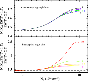
Figure 3: Ratios of the Ni K$\alpha$ line equivalent width (EW) for $\Gamma=1.5$ to the corresponding EW for $\Gamma=2.5$, versus $N_{\rm H}$. Curves are shown for each of the 10 $\theta_{\rm obs}$ bins and are color coded with the same scheme as in Fig. 1 and Fig. 2, and labeled by the angle bin number (see Table 1 in MY09). The angle bins correspond to equal solid angle intervals in the range $0^{\circ}$ to $90^{\circ}$. The upper panel shows angle bins 1–5, corresponding to lines-of-sight that do not intercept the torus, and the lower panel shows angle bins 6–10 corresponding to lines-of-sight that intercept the torus. Note that the vertical axis scale is different for the two panels. The dashed line shows the optically-thin limiting value of the EW ratio, obtained from equation 3.

The EW versus $N_{\rm H}$ curves have an explicit dependence on the assumed opening angle of the torus. This is because different opening angles correspond to different solid angles subtended by the torus at the source and to different projection-angle effects. In the optically-thin regime, this dependence is linear. In the Compton-thick regime, there is a more complicated dependence that must be determined by additional Monte Carlo simulations, which will be the subject of future investigation.

5 Ni K$\alpha$ line Compton shoulder

In addition to the zeroth-order (unscattered) core of the Ni K$\alpha$ emission line, the shape and relative magnitude of the scattered component of the Ni K$\alpha$ emission line (i.e. the Compton shoulder) are also sensitive to the properties of the reprocessor (e.g., see Sunyaev & Churazov 1996; Matt 2002; Watanabe et al. 2003; Yaqoob & Murphy 2010). Fig. 4 shows plots of the ratio of the total number of scattered Ni K$\alpha$ line photons to zeroth-order Ni K$\alpha$ line photons (hereafter, CS ratio) versus $N_{\rm H}$. The ratios are shown for an input power-law continuum with $\Gamma=1.9$, for the face-on and edge-on inclination angle bins (see Table 1 in MY09). It can seen that the CS ratio peaks at $N_{\rm H}\sim 2-3\ \times 10^{24}\ \rm cm^{-2}$, reaching a maximum of $\sim 0.22$ (face-on), and $\sim 0.26$ (edge-on). These are $\sim 75\%$ and $\sim 70\%$ of the corresponding ratios for the Fe K$\alpha$ line (see MY09 and Yaqoob & Murphy 2010). For the face-on inclination angle, the CS ratio for the Ni K$\alpha$ line remains at $\sim 0.22$ once the maximum is reached (even if the column density is increased further) since the Compton shoulder photons escape from within a Compton-depth or so from the illuminated surfaces of the torus for lines-of-sight that are not obscured. For the edge-on inclination angle the CS ratio for the Ni K$\alpha$ line declines as a function of column density after reaching its maximum value, due to a higher probability of absorption at higher column densities.

Figure 4: The ratios of the total number of scattered Ni K$\alpha$ line photons to the number of zeroth-order Ni K$\alpha$ line photons, versus $N_{\rm H}$. Ratios are shown for an input power-law continuum with $\Gamma=1.9$, for the face-on inclination angle bin (lower curve) and the edge-on inclination angle bin (upper curve).

We found that for all values of $\theta_{\rm obs}$ for the torus, there was no detectable difference in the CS ratio as a function of $\Gamma$ up to the $N_{\rm H}$ value that gives the maximum CS ratio (for a given value of $\theta_{\rm obs}$). After that, the CS ratios diverge for different values of $\Gamma$, with flatter incident continua giving larger CS ratios. For the face-on inclination angle the CS ratio at $N_{\rm H}=10^{25}\ \rm cm^{-2}$ varies between $\sim 0.21$ to $\sim 0.22$ as $\Gamma$ varies from 2.5 to 1.5. For the edge-on case, the CS ratio at $N_{\rm H}=10^{25}\ \rm cm^{-2}$ varies between $\sim 0.22$ to $\sim 0.23$ as $\Gamma$ varies from 2.5 to 1.5. Flatter spectra have relatively more continuum photons at higher energies so that the Ni K$\alpha$ line photons are produced deeper in the medium, increasing the average Compton depth for zeroth-order line photons to scatter before escaping. These variations in the CS ratio with $\Gamma$ are likely to be too small to be detectable in practice.

The shape of the Compton shoulder of a fluorescent emission-line escaping from the torus also has a dependence on the column density and inclination angle of the torus. We found that the shapes of the Compton shoulder profiles for the Ni K$\alpha$ line are practically indistinguishable from the shapes of the Fe K$\alpha$ line Compton shoulder profiles (see MY09 and Yaqoob & Murphy 2010). Fig. 5 illustrates the shapes of the Ni K$\alpha$ line Compton shoulder (solid lines) for a power-law incident continuum with $\Gamma=1.9$, for two column densities ($10^{24}$ and $10^{25}\rm\ cm^{-2}$) and two inclination angles of the torus (face-on and edge-on). Corresponding Compton shoulder profiles are also shown for the Fe K$\alpha$ line (dotted lines) for comparison. The Compton shoulder shapes shown in Fig. 5 have no velocity broadening applied to them. The Compton shoulders are shown in wavelength space in units of the dimensionless Compton wavelength shift with respect to the zeroth-order rest-frame energy of the emission line. In other words, if $E$ is the energy of a line photon, and $E_{0}$ is the zeroth-order line energy, $\Delta\lambda=(511\ {\rm keV}/E)-(511\ {\rm keV}/E_{0})$. In order to facilitate a direct comparison of the Compton shoulder profile shapes for different column densities and inclination angles, all of the profiles in Fig. 5 have been normalized to a total flux of unity. It should be remembered that the absolute flux of the Compton shoulder varies significantly with column density, and the flux ratio for two column densities can be estimated using Fig. 4.

Figure 5: The Ni K$\alpha$ emission-line Compton shoulders (solid curves) for a power-law incident continuum with $\Gamma=1.9$, for two column densities and two inclination angle bins, as indicated ($N_{\rm H}=10^{24}$ and $10^{25}\rm\ cm^{-2}$, each for face-on and edge-on orientations of the torus). The dotted curves show the corresponding Compton shoulder profiles for the Fe K$\alpha$ emission line, for the same column densities and inclination angles. No velocity broadening has been applied. Note that in order to directly compare the Compton shoulder shapes, the total flux for each shoulder has been renormalized to the same value. The line flux (in units of normalized flux per unit wavelength shift) is plotted against the dimensionless Compton wavelength shift with respect to the zeroth-order rest-frame energy of the emission line ($E_{0}$), $\Delta\lambda=(511\ {\rm keV}/E)-(511\ {\rm keV}/E_{0})$.

Yaqoob & Murphy (2010) discussed the dependence of the shape of the Fe K$\alpha$ line Compton shoulder on $N_{\rm H}$ and inclination angle in considerable detail. Differences in the shapes of the Compton shoulder profiles for the Ni K$\alpha$ line and the Fe K$\alpha$ line for the same model parameters only become apparent for $N_{\rm H}\gg 10^{24}\ \rm cm^{-2}$ and edge-on inclination angles. However, even at $N_{\rm H}=10^{25}\ \rm cm^{-2}$, the differences are less than $15\%$. Therefore, since the shapes of the Compton shoulder profiles for the Ni K$\alpha$ line are similar to the Fe K$\alpha$ line Compton shoulder profiles within the statistical uncertainties of the Monte Carlo simulations, we do not discuss the Ni K$\alpha$ line Compton shoulder further. The discussion and interpretation of the Fe K$\alpha$ line Compton shoulder in Yaqoob & Murphy (2010) can be applied to the Ni K$\alpha$ line.

6 Summary

We have presented some new results for the flux and EW of the Ni K$\alpha$ fluorescent emission line from Monte Carlo simulations of a toroidal reprocessor illuminated by a power-law X-ray continuum. Our results cover values of the equatorial column density, $N_{\rm H}$, of $10^{22}\rm\ cm^{-2}$ to $10^{25}\rm\ cm^{-2}$, and the calculations were performed for a global covering factor of 0.5 and cosmic elemental abundances. As might be expected, the behavior of the Ni K$\alpha$ line flux and EW as a function of the column density and inclination angle of the torus is similar to that of the Fe K$\alpha$ line. However, the EW of the Ni K$\alpha$ line is a factor of $\sim 22$ smaller than that of the Fe K$\alpha$ in the Compton-thin regime. In the Compton-thick regime, the EW of the Ni K$\alpha$ line reaches a maximum of $\sim 3$ eV for lines-of-sight that do not intercept the torus. For intercepting lines-of-sight the Ni K$\alpha$ EW can be as high as $\sim 250$ eV. The ratio of the Fe K$\alpha$ to Ni K$\alpha$ line EW in the Compton-thick regime, for intercepting lines-of-sight, can be significantly less than the optically-thin limit, as low as $\sim 6$. The above results pertain to an incident power-law X-ray continuum with a photon index of 1.9. Flatter continua give larger EWs and steeper continua give smaller EWs. Varying $\Gamma$ in the range $\Gamma=1.5$ to 2.5 can change the Ni K$\alpha$ EW by up to $\sim 70\%$ in the Compton-thick regime.

We have given analytic expressions for the Ni K$\alpha$ flux and EW in the optically-thin limit. We have also given simple analytic expressions, in the optically-thin limit, for the ratio of the Fe K$\alpha$ to Ni K$\alpha$ line flux, as well as the ratio of the Fe K$\alpha$ to Ni K$\alpha$ line EW. Both of these ratios are independent of the geometry and covering factor of the reprocessor. Moreover, we have found that the ratio of the Fe K$\alpha$ to Ni K$\alpha$ line EW is independent of $\Gamma$, depending only on the Fe to Ni abundance ratio (in the optically-thin limit).

We have also investigated the Compton shoulder of the Ni K$\alpha$ line and we found that the ratio of the flux in the Compton shoulder to that in the zeroth-order component of the line has a maximum value of $\sim 0.22$ and $\sim 0.26$ for face-on and edge-on inclination angles respectively. These are less than the corresponding maxima for the Fe K$\alpha$ line. However, we have found that the shapes of the Ni K$\alpha$ and Fe K$\alpha$ line Compton shoulder profiles are indistinguishable within the statistical accuracy of the Monte Carlo results, except for edge-on inclination angles and $N_{\rm H}\gg 10^{24}\ \rm cm^{-2}$. However, even for $N_{\rm H}$ as high as $10^{25}\ \rm cm^{-2}$, the differences are less than $15\%$.

Our calculations of the Ni K$\alpha$ line flux, EW, and Compton shoulder are meant to serve as a baseline reference because the detailed results, especially in the Compton-thick regime, depend on a number of factors that have not been investigated here. The opening angle of the torus (or effective covering factor) may of course be different to the value used in the calculations. Also, as suggested by Lubinski et al. (2010), part of the torus may be shielded from the X-ray continuum by the accretion disk. However, quantifying this is subject to uncertainties in the geometry of the X-ray source and accretion disk system. Further deviations from the baseline model could occur if the torus does not have a circular cross-section and/or if the torus is clumpy (e.g., Krolik & Begelman 1988; Nenkova, Ivezić & Elitzur 2002). Extension of the parameter space for our model will be the subject of future work.

Acknowledgments
Partial support (TY) for this work was provided by NASA through Chandra Award TM0-11009X, issued by the Chandra X-ray Observatory Center, which is operated by the Smithsonian Astrophysical Observatory for and on behalf of the NASA under contract NAS8-39073. Partial support (TY) from NASA grants NNX09AD01G and NNX10AE83G is also acknowledged. The authors thank Andrzej Zdziarski for helpful comments for improving the paper.

References

- [1] Anders E., Grevesse N., 1989, Geochimica et Cosmochimica Acta 53, 197
- [2] Bambynek W., Crasemann B., Fink R. W., Freund H.-U., Mark H., Swift C. D., Price R. E., Rao P. V., 1972, Rev. Mod. Phys., 44, 716
- [3] Bearden J. A., 1967, Rev. Mod. Phys., 39, 78
- [4] Bianchi S., La Franca F., Matt G., Guainazzi M., Jiménez-Bailón E., Longinotti A. L., Nicastro F., Pentericci L., 2008, MNRAS, 389, L52
- [5] Bianchi S., Matt G, Nicastro F., Porquet D., Dubau, J., 2005, MNRAS, 357, 599
- [6] Jiang P., Wang J. X., Wang T. G., 2006, ApJ, 644, 725
- [7] Jiménez-Bailón E., Piconcelli E., Guainazzi M., Schartel N., Rodríguez-Pascual P. M., Santos-Lleó M., 2005, A&A, 435, 449
- [8] Krolik J. H., Begelman M. C., 1988, ApJ, 329, 702
- [9] Levenson N. A., Heckman T. M., Krolik J. H., Weaver K. A., Zycki P. T., 2006, ApJ, 648, 111
- [Lubiński et al.(2010)] Lubiński P., Zdziarski A. A., Walter R., Paltani S., Beckmann V., Soldi S., Ferrigno C., Courvoisier T. J.-L., 2010, MNRAS, 408, 1851
- [10] Markowitz A. et al., 2007, ApJ, 665, 209
- [11] Matt G., 2002, MNRAS, 337, 147
- [12] Matt G., Bianchi S., Guainazzi M., Molendi S., 2004, A&A, 414, 155
- [13] Matt G., Fabian A. C., Reynolds C. S., 1997, MNRAS, 289, 175
- [14] Molendi S., Bianchi S., Matt G., 2003, MNRAS, 343, L1
- [15] Murphy K. D., Yaqoob T., 2009, MNRAS, 397, 1549 (MY09)
- [16] Nenkova M., Ivezić Ž., Elitzur M., 2002, ApJ, 570, L9
- [17] Page K. L., O’Brien P. T., Reeves J. N., Turner M. J. L.-T., 2004, MNRAS, 347, 316
- [Pounds & Vaughan(2006)] Pounds K., Vaughan S., 2006, MNRAS, 368, 707
- [Reynolds et al.(1994)] Reynolds C. S., Fabian A. C., Makishima K., Fukazawa Y., Tamura T., 1994, MNRAS, 268, L55
- [18] Scott P., Asplund M., Grevesse N., Sauval A. J., 2009, ApJ, 691, L119
- [19] Shu X. W., Yaqoob T., Wang J. X., 2010, ApJS, 187, 581
- [20] Sulentic J. W., Marziani P., Zwitter T., Calvani M., Dultzin-Hacyan D., 1998, ApJ, 501, 54
- [Sunyaev & Churazov(1996)] Sunyaev R. A., Churazov E. M. 1996, Astronomy Letters, 22, 648
- [Torrejón et al.(2010)] Torrejón J. M., Schulz N. S., Nowak M. A., Kallman T. R., 2010, ApJ, 715, 947
- [21] Verner D. A., Ferland G. J., Korista K. T., Yakovlev D. G., 1996, ApJ, 465, 487
- [22] Verner D. A., Yakovlev D. G., 1995 A&AS, 109, 125
- [23] Watanabe S., Sako M., Ishida M. et al., 2003, ApJ, 597, 37
- [24] Weaver. K. A., Gelbord J., Yaqoob T. 2001, ApJ, 550, 261
- [Yang et al.(2009)] Yang Y., Wilson A. S., Matt G., Terashima Y., Greenhill L. J., 2009, ApJ, 691, 131
- [25] Yaqoob T., George I. M., Kallman T. R., Padmanabhan U., Weaver K. A., Turner T. J. 2003, ApJ, 596, 85
- [26] Yaqoob T., George I. M., Nandra K., Turner T. J., Serlemitsos P. J., Mushotzky R. F., 2001, ApJ, 546, 759
- [27] Yaqoob T., Murphy K. D., 2010, MNRAS, in press, arXiv:1010.5262
- [Yaqoob et al.(2010)] Yaqoob T., Murphy K. D., Miller L., Turner T. J., 2010, MNRAS, 401, 411
- [28] Yaqoob T., Padmanabhan U. 2004, ApJ, 604, 63
- [29] Zhou X. L., Wang J. M., 2005, ApJ, 618, L83