FTUV–10–1109

KA–TP–33–2010

SFB/CPP-10-96

IFUM-967-FT

NLO QCD corrections to $W^{\pm}Z\gamma$ production with leptonic decays
G. Bozzi¹, F. Campanario², M. Rauch², H. Rzehak² and D. Zeppenfeld^{2 1} Dipartimento di Fisica, Universita’ di Milano and INFN, Sezione di Milano,
20133 Milan, Italy
² Institut für Theoretische Physik, Karlsruhe Institute of Technology,
Universität Karlsruhe, 76128 Karlsruhe, Germany

We present a computation of the ${\cal O}(\alpha_{s})$ QCD corrections to $W^{\pm}Z\gamma$ production at the Large Hadron Collider. The photon is considered as real, and we include full leptonic decays for the $W$ and $Z$ bosons. Based on the structure of the VBFNLO program package, we obtain numerical results through a fully flexible Monte Carlo program, which allows to implement general cuts and distributions of the final-state particles. The NLO QCD corrections are sizable and strongly exceed the theory error obtained by a scale variation of the leading-order result. Also, the shapes of relevant observables are significantly altered.

1 Introduction

At the LHC a new energy frontier is reached, which allows for new searches of unknown particles and further tests of the Standard Model. From the theory side this also requires very precise predictions of cross sections and distributions, exceeding the precision of a leading-order approximation. We present a calculation of $W^{\pm}Z\gamma$ production including QCD corrections and the leptonic decays of the $W$- and the $Z$-boson with off-shell effects,

$$pp,p\bar{p} \rightarrow W^{\pm}Z\gamma+X\rightarrow\ell_{1}^{\pm}\stackrel{{\scriptstyle\text{\tiny(}-\text{\tiny)}}}{{\nu_{1}}}\ell_{2}^{+}\ell_{2}^{-}\gamma+X\,.$$ (1.1)

This process with leptons, photons and missing energy in the final state provides a background to new physics searches (see, for example, Ref. [1]). Also, this process offers the possibility to study the quartic vector-boson couplings $WWZ\gamma$ and $WW\gamma\gamma$ (see right diagram in Fig. 1) [2] and test the Standard Model. It is one of the missing pieces for a full knowledge of triple vector boson production at next-to leading order (NLO) QCD. There has been a strong effort for the calculation of these processes. The processes with only massive vector bosons in the final state have been completely calculated [3, 4, 5, 6]. Rather recently, also the NLO QCD calculation of the processes $WW\gamma$ and $ZZ\gamma$ have been completed [7] and first results of the NLO QCD computation of the process $W\gamma\gamma$ have been presented [8]. Vector-boson pair production accompanied with one jet has also been studied including QCD corrections for $WWj$, $W\gamma j$, $WZj$ and $ZZj$ [9, 10, 11, 12, 13].

2 Calculational Details

We calculate all contributions to the processes (1.1) up to order $\alpha_{s}\alpha^{5}$ in the limit where all fermions are massless. At leading order, 71 distinct diagrams appear, which we group as three different topologies, according to the number of vector bosons attached to the quark line. An example of each class is depicted in Fig.1.

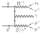
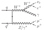
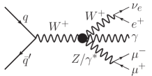
Figure 1: Examples of the three topologies of Feynman diagrams contributing to the process $pp\to$$W^{\pm}Z\gamma$+ X   at tree-level. In the right-hand diagram, the quartic coupling is marked with a dot.

For the last two topologies we also include the cases where vector bosons are radiated off the lepton lines.

To speed up the calculation, invariant subparts, which appear multiple times in different Feynman graphs, are computed only once per phase-space point and independently of the rest of the cross-section. Hereby, we use the procedure of leptonic tensors, as first described in Ref. [14]. This greatly reduces the computation time needed. For the computation of the matrix elements, we use the helicity method introduced in Ref. [15]. Furthermore, by charge conservation, a $W$ boson must always couple to the quark line. Hence, we only need to compute the left-handed chirality part.

At NLO QCD, virtual and real emission diagrams contribute to the cross section. Both contain infrared divergences, which must cancel in the sum according to the Kinoshita-Lee-Nauenberg (KLN) theorem [16]. To handle this cancellation in a numerically stable way, we use the Catani-Seymour dipole subtraction method [17]. Initial-state collinear singularities are partly factorized into the parton-distribution functions. This leads to additional so-called “finite collinear terms”.

The NLO real corrections are given by diagrams where an additional gluon is attached to the quark line which is possible in two different ways. Either this gluon is a final-state particle and considered as radiated off the quark line, or an initial-state gluon which splits into a $q\bar{q}$ pair and we have an emission of a quark. With 194 different Feynman diagrams, the use of leptonic tensors proves to be an advantage in this case.

The presence of isolated on-shell photons requires extra care in the case of real emissions. An additional singularity arises from photon emission collinear to a massless quark. Requiring a simple separation cut between photon and jet is not allowed, since the cancellation of the gluonic infrared divergences between virtual and real emission processes would be spoiled. The phase space for soft-gluon emission would be reduced while leaving untouched the virtual counterpart, leading to the non-cancellation. In principle, this problem can be solved by adding processes with quark fragmentation to photons. Here, we use a simpler approach by requiring a specially crafted cut first suggested in Ref. [18]. We will discuss the details of this cut in section 3.

Virtual NLO QCD corrections arise from the insertion of gluon lines into the topologies of Fig. 1 in every possible way. Therefore, the left topology gives rise to loops with up to five external particles, i.e. pentagon diagrams. For the middle and right ones at most box and triangle diagrams, respectively, appear. Up to the box level, we compute the loop integrals using Passarino-Veltman reduction [19]; additionally we avoid the explicit calculation of the inverse of the Gram matrix. Instead, we solve a system of linear equations, which is numerically more stable close to the singular points. For the pentagon contributions, we apply the method of Ref. [20]. This circumvents the appearance of small Gram determinants in planar configurations of the external momenta altogether. The complete virtual corrections

$$M_{V}=\widetilde{M}_{V}+\ \frac{\alpha_{S}}{4\pi}\ C_{F}\ \left(\frac{4\pi\mu^{2}}{Q^{2}}\right)^{\epsilon}\ \Gamma{(1+\epsilon)}\ \left[-\frac{2}{\epsilon^{2}}-\frac{3}{\epsilon}-8+\frac{4\pi^{2}}{3}\right]\ M_{B},$$ (2.1)

can be separated into a part which is proportional to the Born matrix element, $M_{B}$, and a remainder, $\widetilde{M}_{V}$. Here, $Q$ denotes the partonic center-of-mass energy, which corresponds to the invariant mass of the $WZ\gamma$ final state. For diagrams with only a single $W$ attached to the quark line, $\widetilde{M}_{V}$ vanishes, i.e. the virtual corrections completely factorize to the Born amplitude.

For this factorization formula to hold, the transversality property of the photon $\epsilon(p_{\gamma})\cdot p_{\gamma}=0$ must be used [7]. Then we can reuse the general results for the finite remainder already obtained in Refs. [5, 7], adapting the attached vector bosons to our case. Another optimization can be performed by shifting parts from the pentagon diagrams into box contributions [14, 4, 5, 7]. To do this, we split the polarization vector of the vector bosons into a part proportional to the four-momentum of the boson $q_{V}$ and a remainder $\tilde{\epsilon}_{V}^{\mu}$, which is chosen such that

$$\tilde{\epsilon}_{V}\cdot(q_{W}+q_{Z})=0\,.$$ (2.2)

This part leads to a reduction in the size of the pentagon contributions, which we can therefore compute with lower statistics. Contracting the pentagons with $q_{V}^{\mu}$, they can be expressed as a difference of two box diagrams which are numerically faster to compute. Hence, we can gain speed while keeping the total error the same. This shift also serves as a consistency check between the box and pentagon routines, as the total result must stay unchanged.

To verify the correctness of our calculation, we have performed several checks. First, we have compared all tree-level amplitudes against matrix elements generated by MadGraph[21] and find an agreement of at least 14 digits, which is at the level of the machine precision. Additionally, we have also compared the integrated cross section for both $pp\rightarrow W^{\pm}Z\gamma$ and $pp\rightarrow W^{\pm}Z\gamma j$ against MadEvent and Sherpa [22]. We find an agreement at the per mill level, which is compatible with the integration error. Furthermore, we have checked the implementation of the Catani-Seymour subtraction scheme. We have verified that for the real emission part the ratio between the differential real-emission cross section and the dipole approaches $-1$ once we go to the soft or collinear limit. Also, we have checked that finite contributions left after the cancellation of the infrared divergence can be shifted between the virtual and real parts without affecting the total result.

For the phase space implementation, the $2\rightarrow 5$ phase space was split into three different parts. They correspond to three topologies which we have identified to give the largest contributions, which are of comparable size each. The first one corresponds to a $2\rightarrow 2$ s-channel structure, where possibly a massless particle (the final-state jet for the real-emission contribution) is radiated off first. The two outgoing particles are the massless photon and a pseudo-particle with a mass of 450 GeV and a width of 100 GeV. The latter one then decays into the two massive vector bosons, which in turn decay into their respective fermion–anti-fermion pair, all via $1\rightarrow 2$ topologies. For all invariant masses of intermediate particles we apply a Breit-Wigner mapping to the corresponding random number, so that the peak is flattened out, integrating over the whole available energy range. The second and third structure correspond to $2\rightarrow 2$ s-channel production of the two massive vector bosons, where one undergoes a two-body decay into its fermions and the other one, via a $1\rightarrow 3$ process, into the fermions and the photon. To avoid double-counting we compute for both fermion–anti-fermion pairs the difference of the invariant mass of the photon and the fermion–anti-fermion pair and the mass of the corresponding vector boson. If both differences are larger than 30 GeV, the phase-space point is assigned to the first topology, otherwise to that one where the difference is smaller.

3 Results

We perform the numerical evaluation of our calculation with an NLO Monte Carlo program based on the structure of the VBFNLO program package [23]. As input parameters in the electroweak sector we take the $W$ and $Z$ boson masses and the Fermi constant. The weak mixing angle and the electromagnetic coupling constant are computed from these using tree-level relations:

$$m_{W}=80.398\ \mathrm{GeV} \sin^{2}{(\theta_{W})}=0.22264$$

$$m_{Z}=91.1876\ \mathrm{GeV} \alpha^{-1}=132.3407$$

$$G_{F}=1.16637\cdot 10^{-5}\ \mathrm{GeV}^{-2}\;.$$ (3.1)

Top-quark effects are not considered and all other quarks are taken massless. Effects from generation mixing are neglected, as we set the CKM matrix to the identity matrix. As the central value for factorization and renormalization scales we choose the invariant mass of the leptons and the photon

$$\mu_{F}=\mu_{R}=\mu_{0}=m_{WZ\gamma}\equiv\sqrt{(p_{\ell_{1}}+p_{\nu_{1}}+p_{\ell_{2}}+p_{\bar{\ell}_{2}}+p_{\gamma})^{2}}.$$ (3.2)

For the parton distribution functions, we choose CTEQ6L1 at LO and the CTEQ6M set with $\alpha_{S}(m_{Z})=0.1176$ at NLO [24].

We impose the following set of minimal cuts on the rapidity $y$ and the transverse momentum, $p_{T}$, of the final-state photon and charged leptons

$$p_{T_{\gamma}} >10\ \mathrm{GeV} p_{T_{\ell}} >20\ \mathrm{GeV} |y_{\gamma}| <2.5 |y_{\ell}| <2.5\ .$$ (3.3)

These take into account typical requirements of the experimental detectors. Furthermore, leptons, photon and jet need to be well separated in order to avoid divergences from collinear photons and to be able to identify them as separate objects in the detectors. Therefore, we impose

$$R_{\ell\ell} >0.3 R_{\ell\gamma} >0.4 R_{j\ell} >0.4 R_{j\gamma} >0.4 m_{\ell\ell} >15\ \mathrm{GeV}\ .$$ (3.4)

Here, a jet refers to a final-state quark or gluon in the NLO real emission contribution with $p_{T_{j}}>20$ GeV and $|y_{j}|<4.5$. The last cut in Eq. (3.4) eliminates the singularity from a virtual photon $\gamma^{*}\rightarrow\ell^{+}\ell^{-}$ by requiring that the invariant mass of each pair of oppositely charged leptons is larger than 15 GeV. For treating the collinear singularity between the photon and a parton $i$, we use the procedure of Ref. [18]. The event is accepted only if

$$p_{T_{i}}\leq p_{T_{\gamma}}\frac{1-\cos R_{\gamma i}}{1-\cos\delta_{0}}\text{\quad or\quad}R_{\gamma i}>\delta_{0}\ ,$$ (3.5)

where $\delta_{0}$ is a fixed separation parameter which we set to $0.7$. Eq. (3.5) allows final-state partons arbitrarily close to the photon axis as long as they are soft enough. Thereby, it retains the full QCD pole, which cancels against the virtual part, but it does not introduce divergences from the electroweak sector.

LHC	$\sqrt{s}=$7 TeV			$\sqrt{s}=$14 TeV
	LO[fb]	NLO [fb]	K-factor	LO[fb]	NLO [fb]	K-factor
$4\,\sigma("W^{+}Z\gamma"\to e^{+}\nu_{e}\mu^{+}\mu^{-}\gamma)$
$~{}~{}p_{T_{\gamma(\ell)}}>10(20)$ GeV	0.650	1.075	1.65	1.324	2.441	1.84
$~{}~{}p_{T_{\gamma(\ell)}}>20(20)$ GeV	0.278	0.482	1.74	0.587	1.169	1.99
$4\,\sigma("W^{-}Z\gamma"\to e^{-}\bar{\nu}_{e}\mu^{+}\mu^{-}\gamma)$
$~{}~{}p_{T_{\gamma(\ell)}}>10(20)$ GeV	0.352	0.621	1.76	0.886	1.717	1.94
$~{}~{}p_{T_{\gamma(\ell)}}>20(20)$ GeV	0.146	0.275	1.88	0.381	0.813	2.13

Table 1: Total cross sections at the LHC with center-of-mass energies of 7 and 14 TeV for $pp\to$ $W^{\pm}Z\gamma$$+X$ with leptonic decays, at LO and NLO, and for two sets of cuts. Relative statistical errors of the Monte Carlo are at the per mill level. The factor 4 accounts for all combinations of final-state first- and second-generation leptons.

Tevatron ($\sqrt{s}=1.96$ TeV)	LO[ab]	NLO [ab]	K-factor
$4\,\sigma("W^{\pm}Z\gamma"\to e^{\pm}\stackrel{{\scriptstyle\text{\tiny(}-\text{\tiny)}}}{{\nu}}_{e}\mu^{+}\mu^{-}\gamma)$
$~{}~{}p_{T_{\gamma(\ell)}}>10(10)$ GeV	250.0	370.8	1.48
$~{}~{}p_{T_{\gamma(\ell)}}>20(10)$ GeV	107.4	160.1	1.49

Table 2: Total cross sections at the Tevatron for $p\bar{p}\to$ $W^{+}Z\gamma$$+X$ or $p\bar{p}\to$ $W^{-}Z\gamma$$+X$ including leptonic decays, at LO and NLO, and for two sets of cuts. Relative statistical errors of the Monte Carlo are below the per mill level. The factor 4 accounts for all combinations of final-state first- and second-generation leptons.

In Tables 1 and 2, we present results for the integrated cross section of $W^{\pm}Z\gamma$ production for the LHC with a center-of mass energy of both $7$ and $14$ TeV and for the Tevatron with its center-of-mass energy of $1.96$ TeV. Note, for the Tevatron, the cross section for $W^{+}Z\gamma$ and $W^{-}Z\gamma$ production is the same; the given number is the individual result of one of them. Besides the standard cut on $p_{T_{\gamma}}$ of 10 GeV we also show results for 20 GeV. For the Tevatron, we have reduced the cut on $p_{T_{\ell}}$ to 10 GeV throughout. The cross sections shown correspond to the production of both electrons and muons for all leptons. Interference effects from identical leptons in the final state are neglected, since their contribution is small.

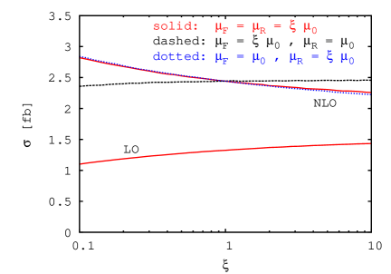
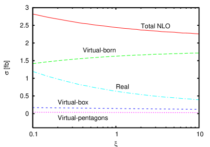
Figure 2: Left: Scale dependence of the total LHC cross section at $\sqrt{s}=14$ TeV for $pp\to W^{+}Z\gamma+X\to\ell_{1}^{+}\ell_{2}^{+}\ell_{2}^{-}\gamma+p\hskip-5.03125pt\hbox to5.03125pt{\hss$/$\hss}_{T}+X$ at LO and NLO within the cuts of Eqs. (3.3, 3.4, 3.5). The factorization and renormalization scales are together or independently varied in the range from $0.1\cdot\mu_{0}$ to $10\cdot\mu_{0}$. Right: Same as in the left panel but for the different NLO contributions at $\mu_{F}=\mu_{R}=\xi\mu_{0}$ with $\mu_{0}=m_{WZ\gamma}$.

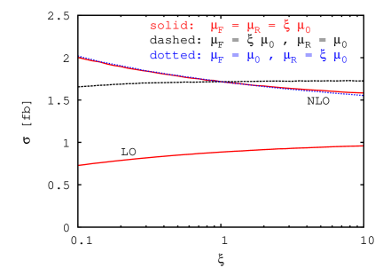
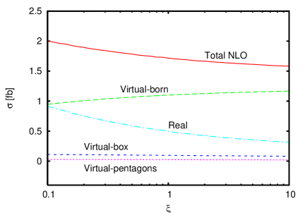
Figure 3: Left: Scale dependence of the total LHC cross section at $\sqrt{s}=14$ TeV for $pp\to W^{-}Z\gamma+X\to\ell^{-}_{1}\ell^{+}_{2}\ell^{-}_{2}\gamma+p\hskip-5.03125pt\hbox to5.03125pt{\hss$/$\hss}_{T}+X+X$ at LO and NLO within the cuts of Eqs. (3.3, 3.4, 3.5). The factorization and renormalization scales are together or independently varied in the range from $0.1\cdot\mu_{0}$ to $10\cdot\mu_{0}$. Right: Same as in the left panel but for the different NLO contributions at $\mu_{F}=\mu_{R}=\xi\mu_{0}$ with $\mu_{0}=m_{WZ\gamma}$.

From hereon, we will focus on the LHC with a center-of-mass energy of 14 TeV. In Figs. 2 and 3 we show the dependence of the cross section for $W^{+}Z\gamma$ and $W^{-}Z\gamma$ production, respectively, when varying the renormalization and factorization scale in the interval

$$\mu_{F},\mu_{R}=\xi\cdot\mu_{0}\quad(0.1<\xi<10)$$ (3.6)

around the central scale $\mu_{0}$ given in Eq. (3.2). We see that the variation of the LO cross section with the scale strongly underestimates the size of the NLO contributions. At the central scale, we obtain a K-factor of $1.84$ for $W^{+}Z\gamma$ and $1.94$ for $W^{-}Z\gamma$. The dependence on the factorization scale slightly reduces when we move from a LO calculation to NLO as expected. On the other hand, the dependence on the renormalization scale shows a large variation. This is due to the fact that $\alpha_{s}$ enters the cross section only at NLO, where we observe the typical leading renormalization scale dependence. When varying the factorization and the renormalization scale jointly by a factor 2 around the central scale $\mu_{0}$, we see a change of 7.5% at LO and 6.7% at NLO for $W^{+}Z\gamma$. For $W^{-}Z\gamma$, the numbers change only slightly to 7.7% and 7.3% for LO and NLO, respectively.

On the right-hand side of Figs. 2 and 3, we show the combined factorization and renormalization scale dependence of the NLO cross section split into the individual contributions. Almost the entire scale dependence is given by the real-emission part, which contains the true real-emission cross section, the dipole terms from the Catani-Seymour subtraction scheme and the finite collinear terms. We obtain the bulk of the NLO contribution from the Born matrix element and the virtual corrections proportional to it. This includes the terms from boxes and pentagons factored out in Eq. (2.1). At the central scale, it is more than twice as large as the real part. The finite virtual remainders due to box and pentagon corrections, which are shifted using Eq. (2.2), only yield a small contribution. The shape of their scale dependence is similar to the one of the total cross section.

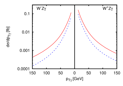
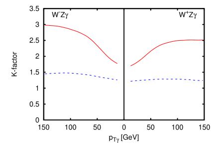
Figure 4: Left: Transverse-momentum distribution of the photon in $W^{+}Z\gamma$  and $W^{-}Z\gamma$  production with leptonic decays of the W- and the Z-boson at the LHC with $\sqrt{s}=14$ TeV. LO (dashed blue line) and NLO (solid red) results are shown for $\mu_{F}=\mu_{R}=\mu_{0}=m_{WZ\gamma}$ and the cuts of Eqs. (3.3, 3.4, 3.5). Right: K-factor for the transverse-momentum distribution of the photon as defined in Eq. (3.7) without (solid red) and including a jet veto of 50 GeV (dashed blue).

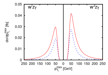
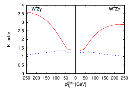
Figure 5: Left: Transverse-momentum distribution of the lepton with largest transverse momentum in $W^{+}Z\gamma$  and $W^{-}Z\gamma$  production with leptonic decays of the W- and the Z-boson at the LHC with $\sqrt{s}=14$ TeV. LO (dashed blue line) and NLO (solid red) results are shown for $\mu_{F}=\mu_{R}=\mu_{0}=m_{WZ\gamma}$ and the cuts of Eqs. (3.3, 3.4, 3.5). Right: K-factor for the maximal-transverse-momentum distribution of the lepton as defined in Eq. (3.7) without (solid red) and including a jet veto of 50 GeV (dashed blue).

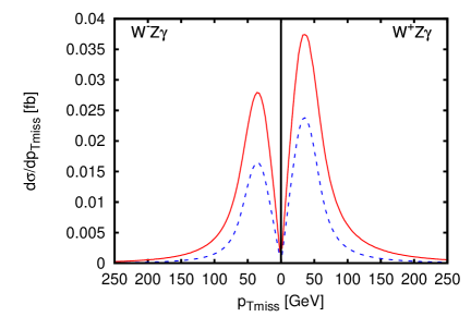
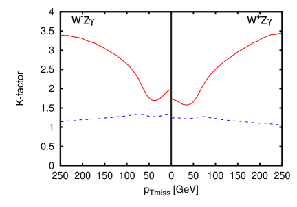
Figure 6: Left: Distribution of missing transverse momentum in $W^{+}Z\gamma$  and $W^{-}Z\gamma$  production with leptonic decays of the W- and the Z-boson at the LHC with $\sqrt{s}=14$ TeV. LO (dashed blue line) and NLO (solid red) results are shown for $\mu_{F}=\mu_{R}=\mu_{0}=m_{WZ\gamma}$ and the cuts of Eqs. (3.3, 3.4, 3.5). Right: K-factor for the missing transverse-momentum distribution as defined in Eq. (3.7) without (solid red) and including a jet veto of 50 GeV (dashed blue).

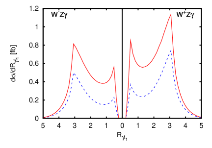
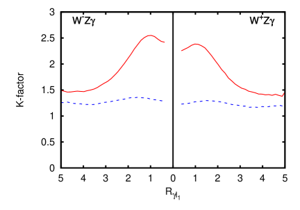
Figure 7: Left: Separation of the photon and the hardest lepton in $W^{+}Z\gamma$  and $W^{-}Z\gamma$  production with leptonic decays of the W- and the Z-boson at the LHC with $\sqrt{s}=14$ TeV. LO (dashed blue line) and NLO (solid red) results are shown for $\mu_{F}=\mu_{R}=\mu_{0}=m_{WZ\gamma}$ and the cuts of Eqs. (3.3, 3.4, 3.5). Right: K-factor for the distribution of the photon-lepton separation as defined in Eq. (3.7) without (solid red) and including a jet veto of 50 GeV (dashed blue).

In Figs. 4, 5 and 6, we show the distribution of the transverse momentum of the photon and the hardest lepton as well as of the missing transverse momentum originating from the neutrino, respectively. On the left-hand side of each figure, we depict the differential cross section at LO and NLO both for $W^{+}Z\gamma$ and $W^{-}Z\gamma$, and on the right-hand side we plot the differential K-factor, defined in the following way:

$$K=\frac{d\sigma^{NLO}/dx}{d\sigma^{LO}/dx}\,\,.$$ (3.7)

We present results which do not include any cut on the additional jet, as well as including a veto on jets with $p_{T_{j}}>50$ GeV. As previously, a jet is defined as a final-state parton with $|y_{j}|<4.5$.

We see that for each of the distributions the K-factor for the differential cross sections without jet veto is not constant, but shows a strong dependence on the momentum scale. In all cases it is close to the integrated one for small values of the transverse momenta coinciding with the bulk of the cross section. For large transverse momenta we observe much bigger K-factors, typically extending up to a value of three. Once we include the additional jet veto, this strong dependence is largely removed. For the transverse-momentum distribution of the hardest lepton in $W^{-}Z\gamma$ for example (Fig. 5), we obtain K-factors between 1.10 and 1.33 over the plotted momentum range. The large differential K-factors are therefore caused by the emission of the additional jet, where the leptonic system recoils against the jet. The integrated K-factors are also reduced, namely to $1.23$ for $W^{+}Z\gamma$ and $1.29$ for $W^{-}Z\gamma$ production.

In Fig. 7, we show the separation in the rapidity–azimuthal-angle plane ($R$ separation) between the photon and the lepton with the largest transverse momentum. Again, we observe a significant dependence of the K-factor on the value of the $R$ separation, varying between $1.4$ and $2.55$. Once we include the jet veto, this dependence is again much smaller.

Therefore, a simple approximation of rescaling the leading-order cross section with the integrated K-factor does not hold. It is necessary to perform a full NLO calculation to reproduce the correct shape of the distributions.

4 Conclusions

We have calculated the NLO QCD corrections to the processes $pp,p\bar{p}\rightarrow W^{\pm}Z\gamma+X$ including full leptonic decays of the $W$ and $Z$ boson. With three leptons, a photon and missing transverse energy as signature, it is an important background for searches for new physics, in particular supersymmetry. Additionally, it can serve as a signal process for measuring the quartic gauge couplings $WWZ\gamma$ and $WW\gamma\gamma$ at the LHC.

We find that the corrections yield a sizable increase of the cross section with respect to the leading-order result, with integrated K-factors typically around $1.9$. The LO scale variation strongly underestimates these contributions with a variation below the $10\%$ level. Varying factorization and renormalization scale $\mu_{F}=\mu_{R}=\mu$ by a factor 2 around the central value $\mu_{0}=m_{WZ\gamma}$, we obtain a remaining scale dependence at NLO of about $7\%$.

The NLO corrections also show a significant dependence on the observable and on different phase-space regions. Therefore, it is important to have a dedicated fully-exclusive NLO parton-level Monte Carlo code available for $W^{\pm}Z\gamma$ production. This process will be included into a future version of the VBFNLO program package.

References

- [1] J. M. Campbell, J. W. Huston and W. J. Stirling, Rept. Prog. Phys. 70, 89 (2007) [arXiv:hep-ph/0611148].
- [2] S. Godfrey, arXiv:hep-ph/9505252; P. J. Dervan, A. Signer, W. J. Stirling and A. Werthenbach, J. Phys. G 26 (2000) 607 [arXiv:hep-ph/0002175]; O. J. P. Eboli, M. C. Gonzalez-Garcia, S. M. Lietti and S. F. Novaes, Phys. Rev. D 63 (2001) 075008 [arXiv:hep-ph/0009262]; P. J. Bell, arXiv:0907.5299 [hep-ph].
- [3] A. Lazopoulos, K. Melnikov and F. Petriello, Phys. Rev. D 76 (2007) 014001 [arXiv:hep-ph/0703273].
- [4] V. Hankele and D. Zeppenfeld, Phys. Lett. B 661 (2008) 103 [arXiv:0712.3544 [hep-ph]].
- [5] F. Campanario, V. Hankele, C. Oleari, S. Prestel and D. Zeppenfeld, Phys. Rev. D 78 (2008) 094012 [arXiv:0809.0790 [hep-ph]].
- [6] T. Binoth, G. Ossola, C. G. Papadopoulos and R. Pittau, JHEP 0806 (2008) 082 [arXiv:0804.0350 [hep-ph]].
- [7] G. Bozzi, F. Campanario, V. Hankele and D. Zeppenfeld, Phys. Rev. D 81, 094030 (2010) [arXiv:0911.0438 [hep-ph]].
- [8] U. Baur, D. Wackeroth and M. M. Weber, PoS RADCOR2009 (2010) 067 [arXiv:1001.2688 [hep-ph]].
- [9] J. M. Campbell, K. R. Ellis and G. Zanderighi, JHEP 0712 (2007) 056 [arXiv:0710.1832 [hep-ph]].
- [10] S. Dittmaier, S. Kallweit and P. Uwer, Phys. Rev. Lett. 100 (2008) 062003 [arXiv:0710.1577 [hep-ph]]; S. Dittmaier, S. Kallweit and P. Uwer, arXiv:0908.4124 [hep-ph].
- [11] F. Campanario, C. Englert, M. Spannowsky and D. Zeppenfeld, Europhys. Lett. 88, 11001 (2009) [arXiv:0908.1638 [hep-ph]].
- [12] F. Campanario, C. Englert, S. Kallweit, M. Spannowsky and D. Zeppenfeld, JHEP 1007 (2010) 076 [arXiv:1006.0390 [hep-ph]].
- [13] T. Binoth, T. Gleisberg, S. Karg et al., Phys. Lett. B683, 154-159 (2010) [arXiv:0911.3181 [hep-ph]].
- [14] B. Jager, C. Oleari and D. Zeppenfeld, JHEP 0607 (2006) 015 [arXiv:hep-ph/0603177]; B. Jager, C. Oleari and D. Zeppenfeld, Phys. Rev. D 73, 113006 (2006) [arXiv:hep-ph/0604200]; G. Bozzi, B. Jager, C. Oleari and D. Zeppenfeld, Phys. Rev. D 75 (2007) 073004 [arXiv:hep-ph/0701105].
- [15] K. Hagiwara and D. Zeppenfeld, Nucl. Phys. B 274 (1986) 1; K. Hagiwara and D. Zeppenfeld, Nucl. Phys. B 313 (1989) 560.
- [16] T. Kinoshita, J. Math. Phys. 3, 650 (1962); T. D. Lee and M. Nauenberg, Phys. Rev. 133, B1549 (1964).
- [17] S. Catani and M. H. Seymour, Nucl. Phys. B 485 (1997) 291 [Erratum-ibid. B 510 (1998) 503] [arXiv:hep-ph/9605323].
- [18] S. Frixione, Phys. Lett. B 429, 369 (1998) [arXiv:hep-ph/9801442].
- [19] G. Passarino and M. J. G. Veltman, Nucl. Phys. B 160 (1979) 151.
- [20] A. Denner and S. Dittmaier, Nucl. Phys. B 658, 175 (2003) [arXiv:hep-ph/0212259]; A. Denner and S. Dittmaier, Nucl. Phys. B 734, 62 (2006) [arXiv:hep-ph/0509141].
- [21] T. Stelzer and W. F. Long, Comput. Phys. Commun. 81 (1994) 357 [arXiv:hep-ph/9401258]; F. Maltoni and T. Stelzer, JHEP 0302 (2003) 027 [arXiv:hep-ph/0208156].
- [22] T. Gleisberg, S. Hoche, F. Krauss, M. Schonherr, S. Schumann, F. Siegert and J. Winter, JHEP 0902 (2009) 007 [arXiv:0811.4622].
- [23] K. Arnold et al., Comput. Phys. Commun. 180 (2009) 1661 [arXiv:0811.4559 [hep-ph]].
- [24] J. Pumplin, D. R. Stump, J. Huston, H. L. Lai, P. Nadolsky and W. K. Tung, JHEP 0207 (2002) 012 [arXiv:hep-ph/0201195].
- [25] J. A. M. Vermaseren, Comput. Phys. Commun. 83 (1994) 45; D. Binosi, J. Collins, C. Kaufhold and L. Theussl, Comput. Phys. Commun. 180, 1709 (2009) [arXiv:0811.4113 [hep-ph]].