The Mass Distribution and Assembly of the Milky Way
from the Properties of the Magellanic Clouds

Abstract

We present a new measurement of the mass of the Milky Way (MW) based on observed properties of its largest satellite galaxies, the Magellanic Clouds (MCs), and an assumed prior of a $\Lambda$CDM  universe. The large, high-resolution Bolshoi cosmological simulation of this universe provides a means to statistically sample the dynamical properties of bright satellite galaxies in a large population of dark matter halos. The observed properties of the MCs, including their circular velocity, distance from the center of the MW, and velocity within the MW halo, are used to evaluate the likelihood that a given halo would have each or all of these properties; the posterior PDF for any property of the MW system can thus be constructed. This method provides a constraint on the MW virial mass, $1.2^{+0.7}_{-0.4}{\rm\,(stat.)}^{+0.3}_{-0.3}{\rm\,(sys.)}\times 10^{12}{\rm M}_{\odot}$ (68% confidence), which is consistent with recent determinations that involve very different assumptions. In addition, we calculate the posterior PDF for the density profile of the MW and its satellite accretion history. Although typical satellites of $10^{12}{\rm M}_{\odot}$ halos are accreted over a wide range of epochs over the last 10 Gyr, we find a $\sim$72% probability that the Magellanic Clouds were accreted within the last Gyr, and a 50%probability that they were accreted together.

1. Introduction

The contents of the Milky Way (MW) Galaxy and the satellites that fall under its dynamical spell provide a unique testbed for theories of galaxy formation and cosmology. Detailed observations of resolved stars, including proper motions, allow the mass distribution of the galaxy to be measured with ever higher precision (e.g. Kallivayalil et al. 2006c; Piatek et al. 2008). Satellite galaxies within the MW have been detected with luminosities three orders of magnitude smaller than in external galaxies (e.g. Belokurov et al. 2007). In addition, determining the detailed phase space distribution of the MW galaxy is critical for interpreting the results of experiments to directly or indirectly detect particle dark matter (e.g. Strigari & Trotta 2009; Vogelsberger et al. 2009; Lisanti et al. 2010; Kuhlen et al. 2010). A full understanding of the MW’s place in the Universe requires not only detailed knowledge of its mass distribution and formation history, but also a sense of how this one well-studied system fits into the full cosmological context.

A variety of methods have been used to put limits on the MW mass, ranging from stellar dynamics and dynamics of satellites (Klypin et al. 2002; Battaglia et al. 2005; Dehnen et al. 2006; Smith et al. 2007; Xue et al. 2008; Watkins et al. 2010; Gnedin et al. 2010) to the dynamics of the local group (Li & White 2008). For example, Battaglia et al. (2005) and Xue et al. (2008) performed a Jeans analysis of measurements of the radial velocity dispersion profile from satellite galaxies, globular clusters, and blue horizontal branch halo stars to estimate the MW radial density profile. Smith et al. (2007) used measurements of high-velocity halo stars to estimate the MW escape speed assuming an NFW profile. Li & White (2008) took a complementary approach, using the relative position and velocity of the MW and M31, along with the age of the universe, to infer properties of the obits of the MW-M31 system, which provides constraints on the total mass.

Similarly, there have been a range of studies on the dynamical state of the Magellanic Clouds (MCs). Until recently, the standard picture was that the MCs were objects that have been orbiting the MW for some time (Murai & Fujimoto 1980; Gardiner et al. 1994). This picture was motivated in part by the presence of the Magellanic Stream, a filament of gas extending $150^{\circ}$ across the sky. Because it is apparently spatially and chemically associated with the Magellanic Clouds, it has often been interpreted as a tidal tail and taken as an indication that the satellites have been around for several Gyr (see, e.g., Lin & Lynden-Bell 1982; Connors et al. 2006). This picture has recently come under fire, largely as a result of detailed measurements of the three-dimensional velocity of the MCs: they are observed to have high velocities not aligned with the Magellanic Stream, indicating that they are not in virial equilibrium (and suggesting alternative formation methods for the Magellanic Stream; see Besla et al. 2007, 2010). Similarly, there is a growing consensus that the MCs accreted as a group: evidence for this comes from both their proximity in phase space (Kallivayalil et al. 2006a), and the result that simulated subhalos in general tend to accrete in groups (D’Onghia & Lake 2008).

In this work, we take a new approach to measure the mass and assembly of the MW. N-body simulations of dark matter structures in a $\Lambda$CDM  universe have been very successful at reproducing the observed clustering of galaxies (e.g. Kravtsov et al. 2004; Conroy et al. 2006; Trujillo-Gomez et al. 2010). In two companion papers, we show that the full probability distribution (PDF) for the number of bright satellites around MW-luminosity hosts predicted by high resolution numerical simulations (Busha et al. 2010) is in excellent agreement with measurements from the SDSS (Liu et al. 2010; Tollerud et al. 2011). This provides evidence that such cosmological simulations realistically represent galaxy halos and their satellites, and that they sample the underlying probability distribution for the properties of halos and subhalos in our Universe. These simulated halo catalogs therefore constitute a highly informative prior PDF for the parameters of any particular galaxy system. In this work we show that combining this prior with basic data about the two most massive MW satellites — their masses, velocities, and positions — provides interesting constraints on the MW mass, the distribution of mass within the MW system, and the system’s assembly history. Although we find that the simulation used here provides only a relatively sparse sampling of the underlying PDF, this is the first time that the statistics to study the MW system in this way have been available at all. As high-resolution cosmological simulations probe ever larger volumes, this approach will have increasing power and applicability.

2. Simulations

Statistical inference from halo dynamical histories requires a large, unbiased set of dark matter halos which samples the full range of cosmologically appropriate formation scenarios. Here, we use halos from the Bolshoi simulation (Klypin et al. 2010), which modeled a 250 $h^{-1}\rm{Mpc}$ comoving box with $\Omega_{m}=0.27$, $\Omega_{\Lambda}=0.73$, $\sigma_{8}=0.82$, $n=0.95$, and $h=0.7$. The simulation volume contained $2048^{3}$ particles, each with mass $1.15\times 10^{8}h^{-1}\hbox{${\rm M}_{\odot}$}$, and was run using the ART code (Kravtsov et al. 1997). Halos and subhalos were identified using the BDM algorithm (Klypin & Holtzman 1997); see Klypin et al. (2010) for details. One unique aspect of this simulation is the high spatial resolution, which is resolved down to a physical scale of 1 $h^{-1}\rm{kpc}$. This improves the tracking of halos as they merge with and are disrupted by larger objects, allowing them to be followed even as they pass near the core of the halo. The resulting halo catalog is nearly complete for objects down to a circular velocity of ${\rm v}_{\rm max}=50$ km $s^{-1}$. While the overall simulation suffers from incompleteness in satellites at the $\sim$ 20% level at 50km $s^{-1}$, the incompleteness is strongly dependent on host mass. Host halos with $\hbox{$M_{\rm vir}$}=0.5-3\times 10^{12}h^{-1}\hbox{${\rm M}_{\odot}$}$ seem to be missing fewer than $\sim 10\%$ of their subhalos. Because we are primarily interested in these lower mass objects, the amount of incompleteness is small and can be ignored.

The large volume probed results in a sample of 2.1 million simulated galaxy halos at the present epoch, including more than 100,000 halos massive enough to host at least one resolved subhalo. We can increase this number further by considering halos identified at different epochs to be independent objects representative of local systems: we use halos from 60 simulation snapshots out to redshift 0.25. Throughout, we define “hosts” as halos that are not within the virial radius of a larger halo, and “satellites” as any object within 300 kpc of a host. This value is chosen to be roughly half the distance between the MW and M31. Note that our final results are largely independent of this choice, because we will later impose more stringent requirements on the distance from the satellites to the center of their host halo.

3. Observations

We now consider the massive subhalo population of the MW that is modeled by the Bolshoi simulation: objects with ${\rm v}_{\rm max}>50$ km $s^{-1}$. The two brightest MW satellite galaxies, the LMC and SMC, have both been measured to have maximum circular velocities ${\rm v}_{\rm max}\lower 2.15277pt\hbox{$\;\buildrel>\over{\sim}\;$}60$ km $s^{-1}$ with magnitudes $M_{V}=-18.5$ and -17.1, respectively (van der Marel et al. 2002; Stanimirović et al. 2004; van den Bergh 2000). The next brightest satellite is Sagittarius, some 4 magnitudes dimmer, with ${\rm v}_{\rm max}\sim 20$ km $s^{-1}$(Strigari et al. 2007). Similar constraints, albeit with larger error bars, can be made for the other bright classical satellites. The census of nearby objects brighter than $M_{V}\approx-8$ should be complete well beyond the MW virial radius (Walsh et al. 2009; Tollerud et al. 2008). It is therefore a robust statement that the MW has exactly two satellites with ${\rm v}_{\rm max}\lower 2.15277pt\hbox{$\;\buildrel>\over{\sim}\;$}50$km $s^{-1}$.

Applying this selection criterion to the Bolshoi catalog, we find 36,000 simulated halos that have exactly two satellites with ${\rm v}_{\rm max}>50$km $s^{-1}$. These $N_{\rm subs}=2$ systems represent a first attempt at finding simulated halos that are analogs of the MW in terms of massive satellite content. What other properties of the LMC and SMC might provide information on the mass and assembly history of the MW system? Repeated observations over many years with HST and ground-based spectroscopy have given us excellent limits on both the 3D position and velocity of both objects. Indeed, both of these properties are significantly better constrained than are the circular velocities of these objects. We select simulated objects to be MC analogs based on $v_{\rm max}$, the maximum circular velocity of the object, $r_{0}$, the distance of the object to the center of the MW, and $s$, the total speed of the object relative to the MW. These are summarized in Table 1. In order to be conservative with the uncertainties to account for systematics, we multiply the published formal errors in the speed by a factor of two when looking for MC analogs in Bolshoi (included in the errors shown in Table 1). This increase is necessary to bring the velocity measurements of the SMC by Kallivayalil et al. (2006b) and Piatek et al. (2008) into agreement.

Note that there is a slight discrepancy between the observational measurements of satellite ${\rm v}_{\rm max}$ and the simulations: while observations measure the circular velocity curve for all components of the halo — dark matter and baryons — the Bolshoi simulation models only the dark matter content. Trujillo-Gomez et al. (2010) showed that ignoring the baryonic component may cause a $\sim 10\%$ over-estimate in the measurement of ${\rm v}_{\rm max}$ for MC-sized objects. Since this correction is smaller than the error bars on the observations, we choose to ignore it. Additionally, there is some disagreement in the literature as to the allowable upper limit for ${\rm v}_{\rm max}$. In particular, some estimates for the LMC are in excess of 100 km/s (Piatek et al. 2008), well above our adopted 80km/s $1\sigma$ upper limit. However, due to the rapidly declining abundance of such massive subhalos (see, e.g., Busha et al. 2010), our analysis is highly insensitive to changes in the upper error bar on ${\rm v}_{\rm max}$. Finally, because of resolution effects, there is a radial dependence to the incompleteness of satellite halos, with the large density contrast and limited force resolution making it difficult to identify subhalos closer to the center of their hosts. However, this incompleteness does not appear to correlate with host mass, so we do not expect it to bias our results.

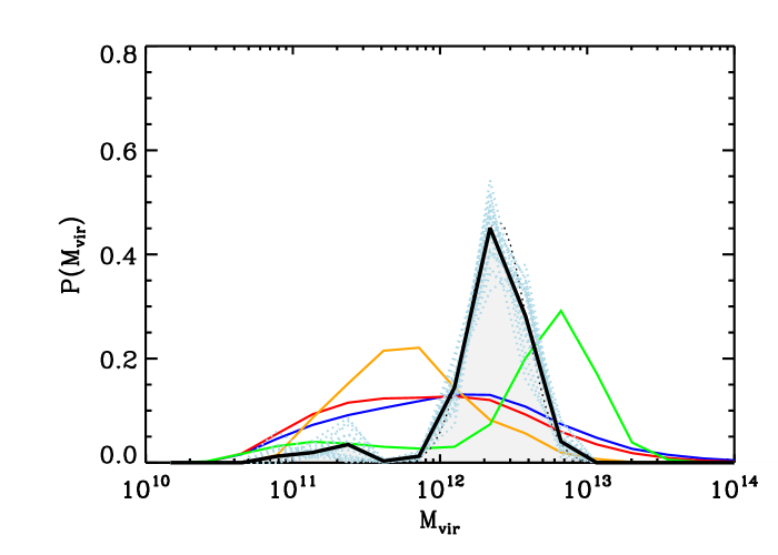
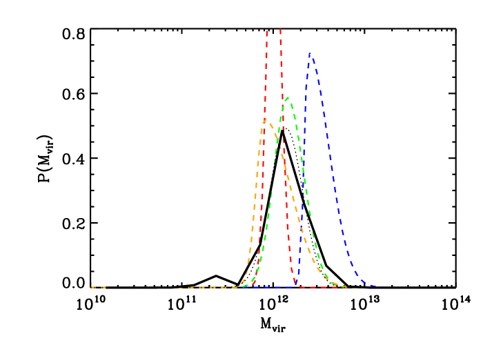
Figure 1.— Left: The MW mass inferred from the properties of its two most luminous satellites, the Magellanic Clouds. Lines show posterior PDFs (weighted histograms of Bolshoi halos) given information about (a) the existence of exactly two satellites with $v_{\rm max}>50$ km s^-1 (blue), (b) the maximum circular velocities $v_{\rm max}$ of the two satellites (red), (c) the distance of each satellite from the center of the MW (orange), (d) the speed of each satellite (green), and (e) all of these properties simultaneously (black). The combined properties define a sample of “satellite analogs” and give ${\rm M}_{\rm MW}=1.2^{+0.7}_{-0.4}{\rm\,(stat.)}^{+0.3}_{-0.3}{\rm\,(sys.)}\times 10^{12}{\rm M}_{\odot}$ (68% confidence). The dotted line shows a lognormal fit to this distribution, with parameters $\log_{10}{{\rm M}_{\rm MW}}=12.2\pm 0.1$, and the dashed gray lines show the effect of bootstrap resampling: the uncertainty on the mean of the distribution from “sampling noise’ in the catalogs was found in this way to be just $0.03$ dex.
Right: Comparison with various estimates for the mass of the MW from the literature. Dashed lines show results from: (a) the radial velocity dispersion profile (Battaglia et al. 2005) (orange); (b) the escape velocity from halo stars (Smith et al. 2007) (red); (c) SDSS blue horizontal branch stars (Xue et al. 2008) (green), and (d) the timing argument (Li & White 2008) (blue). We assume lognormal error distributions, with asymmetric errors given by the quoted upper and lower confidence limits. The solid (black) line shows the posterior PDF for the MW mass from our satellite analogs, and the dotted line again shows thee lognormal fit to this distribution.

Table 1 Observed properties of the LMC and SMC.

	LMC	SMC	Reference
${\rm v}_{\rm max}$ [km/s]	$65\pm 15$	$60\pm 15$	vdM02, S04, HZ06
$r_{0}$ [kpc]	$50\pm 2$	$60\pm 2$	vdM02
$s$ [km/s]∗	$378\pm 36$	$301\pm 104$	K06

Note. — For a given satellite, ${\rm v}_{\rm max}$ is its estimated maximium circular velocity, $r_{0}$ its estimated distance from the Galactic center, and $s$ its estimated speed relative to the Galactic center. References are: vdM02 = van der Marel et al. (2002); S04 = Stanimirović et al. (2004); K06 = Kallivayalil et al. (2006a,2006c) HZ06 = Harris & Zaritsky (2006).
^∗ Errors on $s$ have been increased relative to the published values for conservatism (see text).

4. Inference

The Bolshoi halo catalog is large enough for some of its members to resemble the Milky Way system, with regards to its two most massive satellites. By weighting the Bolshoi halos according to how closely their satellites’ properties match those of the MW’s, we can infer the mass and assembly history of the MW system. In this section we explain how this works, and derive the required weights from probability theory.

4.1. Observational constraints and the likelihood function

As outlined above, the Bolshoi halo catalog can be thought of as a set of samples drawn from an underlying probability distribution. Each halo is characterized by a set of $m$ parameters, $\mathbf{x}$, which includes the total mass of the halo and the properties of its subhalos, such as their masses, positions, and velocities: $x=\left(M_{\rm vir},\{v_{\rm max},r_{0},s,\ldots\}_{\rm LMC,SMC}\right)$. Given no observational data, the set of Bolshoi halos provides a reasonable characterization of our prior PDF for the parameters of the Milky Way system, ${\rm Pr}(\mathbf{x})$. For example, if we were asked to guess the mass of the MW halo, we would do much worse by drawing a random number from some wide range, than we would do by drawing one Bolshoi halo at random from the catalog.

However, we do have some observational data: we would therefore like to know the posterior PDF for the parameters of the Milky Way system, given this data $\mathbf{d}$. Bayes’ theorem shows this to be:

$${\rm Pr}(\mathbf{x}|\mathbf{d})\propto{\rm Pr}(\mathbf{d}|\mathbf{x}){\rm Pr}(\mathbf{x})$$ (1)

The first term on the right hand side is the joint likelihood function for the parameters, written as a function of the data. Given a particular parameter vector $\mathbf{x}$, we can compute the value of this likelihood in the usual way, given assumptions about the error distributions of the observational data. Our data $\mathbf{d}$ and their uncertainties $\sigma$ are given in Table 1: $\mathbf{d}=\left(v_{\rm max}^{\rm obs},r_{0}^{\rm obs},s^{\rm obs}\right)$ (for each MC). We use the superscript “obs” to make clear the distinction between the (constant) measured values, and the corresponding (variable) parameters of the model, which are the properties of the Bolshoi halos. We interpret the errors on the observational data as being Gaussian-distributed, such that for each datum $d_{i}$ its likelihood function ${\rm Pr}(d_{i}|\mathbf{x})$ is a Gaussian, with mean and standard deviation listed in Table 1.

Since the $N=6$ observations were made independently by different groups using different techniques, the joint likelihood is just a simple product:

$${\rm Pr}(\mathbf{d}|\mathbf{x}) = \prod_{i}^{N}{\rm Pr}(d_{i}|\mathbf{x}),$$ (2)

$$= \prod_{\rm LMC,SMC}N(v_{\rm max}^{\rm obs}|v_{\rm max},\sigma_{v}^{2})$$ (4)

$$\;\;\;\;\;\;\;\;\;\;\;\;\;\;\;\;\;\;\;\;\;\times N(r_{0}^{\rm obs}|r_{0},\sigma_{r}^{2})\times N(s^{\rm obs}|s,\sigma_{s}^{2}),$$

where

$$N(y|\mu,\sigma)=\frac{1}{\sigma\sqrt{2\pi}}\exp\left[-\frac{\left(y-\mu\right)^{2}}{2\sigma^{2}}\right]$$ (5)

is the Gaussian probability density in $y$ with mean $\mu$ and variance $\sigma^{2}$.

Conditional on the values of the parameters, the data measurements are independent, and thus the likelihood function factors into the product of N=6 terms. In the prior, the dynamical parameters and halo properties themselves are correlated, and not independent, because of the simulation physics. We have a measurement of satellite distance, $r_{0}^{\rm obs}$, and an independent measurement of satellite velocity $s^{\rm obs}$: the probability calculus makes it very clear that the PDFs for these two observed quantities can be multiplied together, even though the corresponding underlying parameters $r_{0}$ and $s$ are not independently distributed. (We discuss correlations between the measurements of $r_{0}$ and $s$ below.)   The dynamics of satellites around halos is such that their positions and velocities are correlated according to the orbits they are on. This is a good thing: it means that by measuring one we can learn about the other! In fact, it is this very interdependence that will allow us to infer the MW halo mass given measurements of its satellite properties. All the correlations between the model parameters are correctly taken into account by drawing samples from the joint prior PDF – that is, by using the Bolshoi catalog.

4.2. Importance Sampling

With the likelihood function in hand, we can now calculate the posterior PDF for the MW system parameters given our data. We have the prior PDF ${\rm Pr}(\mathbf{x})$ in the form of a set of $n$ samples drawn from it; this is actually a very convenient characterization, and will allow us to derive an equally convenient characterization of the posterior. We compute posterior estimates using importance sampling (see MacKay 2003 for an introduction, and papers by Lewis & Bridle 2002 and Suyu et al. 2010 for example applications in astronomy). In general, this technique involves generating samples from an importance sampling function, which are then weighted when computing integrals over the target PDF. In this paper, we choose the importance sampling function to be the prior PDF, so that the importance weights are proportional to the likelihood; this allows us to compute integrals over the posterior PDF, as shown below.

These integrals include mean parameter values, confidence intervals and so on; a histogram of sample parameter values is a representation of the marginalized distribution for that parameter, and is also a set of integrals (counts of samples in bins).

In general, integrals over the posterior PDF can be written as follows:

$$\int f(\mathbf{x})\,{\rm Pr}(\mathbf{x}|\mathbf{d})\,d^{m}\mathbf{x} = \frac{\int f(\mathbf{x})\,{\rm Pr}(\mathbf{d}|\mathbf{x})\,{\rm Pr}(\mathbf{x})\,d^{m}\mathbf{x}}{\int{\rm Pr}(\mathbf{d}|\mathbf{x})\,{\rm Pr}(\mathbf{x})\,d^{m}\mathbf{x}}$$ (6)

$$\simeq \frac{\sum_{j}^{n}f(\mathbf{x}_{j})\,{\rm Pr}(\mathbf{d}|\mathbf{x}_{j})}{\sum_{j}^{n}{\rm Pr}(\mathbf{d}|\mathbf{x}_{j})}$$ (7)

where in the first line we have substituted for the posterior PDF using equation 1, and in the second line we have approximated the integrals with sums over samples drawn from the prior PDF. The denominator in each case is a normalization constant. $f(\mathbf{x})$ is any function of interest to be integrated: for example, $f(\mathbf{x})=\mathbf{x}$ gives the posterior mean parameters. The highest importance samples correspond to halos that most resemble, in terms of its bright satellite properties, the halo of the MW.

4.3. Assumptions

In this subsection, we examine the assumptions we have made in more detail.

4.3.1 Data covariance

As noted above, the constraints on $r_{0}$ and $s$ are nearly, but not quite, independent. Working in galactic coordinates and following the method outlined in van der Marel et al. (2002), the separation between the MCs and the center of the MW, $r_{0}$, is given by the relation

$$r_{0}^{2}=\hbox{${{\bf r}}_{\odot}$}^{2}+{\bf r}_{e}^{2}+2(\hbox{${{\bf r}}_{\odot}$}\cdot{\bf r}_{e}),$$ (8)

where ${{\bf r}}_{\odot}$ is the location of the center of the galaxy and $\bf{r}_{e}$ location of the MCs, both relative to the sun. Similarly, the speed, $s=|{\bf s}|$, for the MCs is given by

$${\bf s}=\hbox{${{\bf v}}_{\odot}$}+(\mu_{N}{\bf u}_{N}+\mu_{W}{\bf u}_{W})r_{e}+v_{los}{\bf u}_{los},$$ (9)

where ${{\bf v}}_{\odot}$ is the relative motion between the sun and the center of the galaxy, $\mu_{N}$ and $\mu_{W}$ are the measured north and west transverse components of the proper motion of the MCs on the sky, $\bf{v}_{los}$ the measured line of sight velocity of the MCs, and $\bf{u}_{N},\bf{u}_{W}$, $\bf{u}_{los}$ are the unit vectors defining the (north and west) transverse and radial directions of motion of the MCs relative to the sun in galactic coordinates.

As can be seen in equations 8 and 9, $r_{e}$, the distance from the Sun to the MCs, is a necessary measurement for determining both $r_{0}$ and $s$, hence these measurements are not fully independent. In order to determine the degree of dependance, we calculate $\rm{COV}(r_{0},s)$, the covariance between these variables, and and show that this is significantly smaller than the measurement errors on the properties,

$${\rm COV}(r_{0},s)\ll\sigma_{r_{0}}\sigma_{s}.$$ (10)

The covariance can be explicitly written as

$${\rm COV}(r_{0},s) = {dr_{0}\over dr_{e}}{ds\over dr_{e}}\sigma_{r_{e}}=$$

$${1\over\sqrt{r_{0}}}(r_{e}+{\hbox{${{\bf r}}_{\odot}$}\cdot{\bf r}_{e}\over r_{e}}) \times {1\over 2\sqrt{s}}(\mu_{W}^{2}+\mu_{N}^{2})\times\sigma_{r_{e}}$$ (11)

Using values reported in van der Marel et al. (2002) and Kallivayalil et al. (2006a), we measure COV($r_{0},s$) = 6.52 and 6.86 for the LMC and SMC, respectively. In both cases, this at least an order of magnitude smaller than the product $\sigma_{r_{0}}\sigma_{s}=$ 72, and 208, allowing us to treat the measurements of $r_{0}$ and $s$ as independent.

4.3.2 Simulation time resolution

The observational constraints on the positions of the MCs are actually tighter by a factor of two than the resolution of our simulations. The available Bolshoi outputs are such that a satellite with the LMC’s radial velocity of $\simeq 90$ km/s (Kallivayalil et al. 2006c) will travel roughly 4 kpc between sequential snapshots, making this the effective uncertainty on the radial position of the simulated halos. We increase the size of the positional uncertainties accordingly, when calculating the likelihood function for the MC positions.

4.3.3 Importance sampling failure modes

Typically there are two ways in which importance sampling can fail. The first is that the sampling function does not cover the domain of the target PDF, leaving parts of the PDF unsampled. In our case, we assert that the Bolshoi simulation does sample the parameter space, in that it contains (in large numbers) halos and subhalos with masses, positions and velocities sufficiently close to the members of the MW system to make inferences meaningful. The second failure mode is that too few samples are drawn in the high importance volume, leading to estimates dominated by a small number of high importance samples. As we shall see, this “sampling noise” does lead to additional uncertainty on our inferences. Because of the very tight observational constraints on the properties of the MCs, relatively few Bolshoi halos receive significant importance – we can only partially compensate for this by searching through multiple simulation outputs to improve the statistics of our sample. In Sections 5 and 6 below, we estimate the uncertainty, due to sampling noise, on each of our estimates by bootstrap resampling.

4.3.4 The effect of the Galactic disk

Finally, the lack of treatment of baryons in Bolshoi introduces a systematic error. The more concentrated mass in the stellar disk at the halo center should increase the speed of the satellites orbiting their hosts at small radii. We can estimate the impact of this by artificially increasing the total velocity of our simulated satellites by the circular velocity due to the stellar disk of the Milky Way, $v_{circ}=\sqrt{(}GM_{*}/r_{sat})$, where $M_{*}=6\times 10^{10}\hbox{${\rm M}_{\odot}$}$(Klypin et al. 2002). This correction is admittedly simplistic, but is also small. To conservatively quantify the residual systematic error associated with this correction, we take the difference in mass estimates with and without the above correction. This gives us an approximate upper limit on the size of the two-sided systematic error due to baryon physics.

5. The Mass Distribution of the Milky Way

Figure 1 (left panel) shows the posterior PDF for the MW halo mass, computed by weighting every Bolshoi halo by the probability that its bright satellite population looks like that of the MW in various ways. Some observations provide significantly more information about the host halo mass than others: the distance to and speed of the MCs are most constraining, while the maximum circular velocity of the LMC and SMC provide almost no information (largely due to their measurement errors). Note that it is the combination of datasets that is most important, as internal degeneracies are broken, i.e., there is a high degree of covariance between positional and kinematic properties. The combination of all datasets gives ${\rm M}_{\rm MW}=1.2^{+0.7}_{-0.4}{\rm\,(stat.)}^{+0.3}_{-0.3}{\rm\,(sys.)}\times 10^{12}{\rm M}_{\odot}$ (68% confidence) and a virial radius $r_{vir}=250^{+60}_{-30}\rm{kpc}$. The systematic errors are estimated by repeating this process with and without the baryon correction discussed at the end of Section 4.

How many halos contribute to this inference? We find 114 $1\sigma$ matches (systems that are within an average of $1\sigma$ from observations of the MCs in the 6 properties listed in Table 1) and nearly 400 $2\sigma$ matches in the 60 snapshots. However, many more contribute statistically. The effective number of halos contributing to the posterior can be estimated as $N_{\rm eff}=N/(1+{\rm Var}(w))$ (Neal 2001), where $w$ is the normalized importance of each halo and $N$, in our case, is $1.71\times 10^{6}$ (total number of halos over all 60 snapshots). We find $N_{\rm eff}=10,051$.

While this is a healthy number of samples to compute statistics with, the low fraction of halos that contribute is driven largely by the combination of the total speed, $s$, and radial position, $r_{0}$, constraints. This gives additional support to the idea that the MCs are currently at-or-near pericentric passage on their orbits around the Milky Way, since any object on an elliptical orbit spends such a small amount of time near pericenter. Figure 1 shows the effects of the sampling noise on the inference of the MW mass: the faint blue-grey curves show 25 bootstrap-resampled PDFs. The additional uncertainty on the central value is 0.03 in $\log_{10}({\rm M}_{\rm MW})$ – this is included this in the quoted error bars above, which were estimated from the sum of the resampled PDFs.

Figure 1 (right panel) compares our result with previous MW halo mass estimates from the literature. The LMC and SMC properties lead to a halo mass that is in excellent agreement with the dynamical estimates in the literature. In particular, our results are in near perfect agreement with the most recent stellar velocity measurements (Xue et al. 2008), with similar error bars.

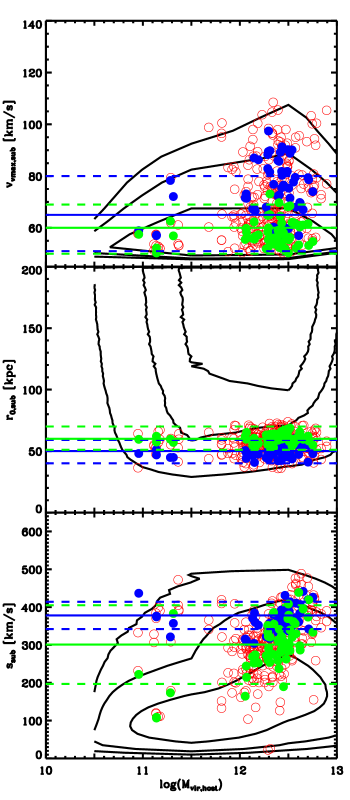
Figure 2.— Relationships between $M_{vir,host}$ and various satellite parameters: ${\rm v}_{\rm max}$ (top left), $r_{0}$ (top right), and $s$ (bottom left). In all panels, the black contours denote the regions containing 68, 90, 95, 98, and 99% of our prior distribution, all satellites in a host with $N_{sub}=2$. The open red and filled circles denote the satellites for 2- and 1-$\sigma$ halos, those that contribute most to the posterior PDF. Blue and green lines show the observed values and $\pm 1-\sigma$ uncertainty for each property, for the LMC and SMC respectively. Similarly, the blue and green circles denote the values for our identified LMC and SMC analogs.

Throughout the paper, we refer to the collection of hosts weighted by the likelihood of the ${\rm v}_{\rm max},r_{0}$, and $s$ of their satellites as “satellite analogs” of the MW. Note that this does not imply that we have selected a specific subset of hosts. Rather, we have taken all hosts with $N_{subs}=2$ and weighted each object by its satellite properties. It is this sample of weighted objects that defines our satellite analogs. It is worth noting, however, while we formally use all 35,000 $N_{subs}=2$ halos in Bolshoi, the $\sim 500$ 1- and 2-$\sigma$ halos provide more than 95% of the total weight.

Because we want to further understand what impact the MCs have on other other halo properties, we also define “mass analogs” to be the set of halos randomly drawn from the mass PDF of the satellite analogs. Thus, the mass analogs have the same PDF of virial masses as the black line of Figure 1, but no constraints on their satellite properties. Comparison between our satellite analogs and mass analogs allows us to disentangle impacts on the system due to the satellite properties from those due to the particular mass range probed by our satellite analogs.

When interpreting Figure 1, it is also helpful to consider the full dependence of the predicted satellite properties on the mass of the host halos. This is shown in Figure 2, which compares the satellite parameters $v_{max,},r_{0}$, and $s$ with the $M_{\rm vir}$ of their hosts. The plots show contours containing 68, 90, 95, 98, and 99% of our prior probability (that is, all hosts with exactly two satellites, black lines), as well as the exact locations of our 2-$\sigma$ (open red circles) and 1-$\sigma$ hosts (filled circles). Also plotted are the observed properties of the LMC and SMC (blue and green lines). These plots highlight a number of important trends. First, we can see that the MCs are atypical subhalos in most regards. The LMC in particular is roughly a 2-$\sigma$ outlier in each of these properties. Second, correlations between parameters can be seen, such as the that between speed and host mass, which shows explicitly how the high observed speed of the satellites skews the posterior PDF towards higher mass hosts. Additionally, it is interesting to note that, while rare, there are a few objects with $\hbox{$M_{\rm vir}$}<10^{11}\hbox{${\rm M}_{\odot}$}$ with satellites that are well matched to the MCs. These satellites are fast moving, massive subhalos roughly 50 and 60 kpc from their host centers – well within their host virial radii, but not energetically bound to their hosts, and hence merely transient events. Finally, while it can be seen that observations of $s$ provide the most stringent constraints individually, these plots further emphasize that it is the combination of observed properties that is necessary to place tight constraints on ${\rm M}_{\rm MW}$.

We can also determine the impact of the MCs on the internal mass distribution of a halo by comparing the density profiles for our satellite and mass analogs. This gives us a handle on how typical the MW is for a halo of its mass. We find that the presence of the MCs has only a modest impact on the halo concentration, but can impact density profiles significantly in other ways. In particular, when looking at the mass enclosed within a fixed 8 kpc (the distance from the sun to the center of the galaxy), satellite analogs have a 60% higher central density than mass analogs. This tells us that the MCs are correlated with a more strongly peaked inner dark matter distribution. For the full density profile (which includes contributions from substructures), however, satellite analogs have concentration $c_{vir}=11\pm 2$, a little less than 1-$\sigma$ higher than $c_{vir}=8.7\pm 3.5$ for the mass analogs (here, $c_{vir}=r_{vir}/r_{s}$). While this still implies a correlation between the presence of the MCs and a more peaked mass distribution, it shows that the impact is much weaker at larger radii than it is for the central core.

6. The Assembly of the Milky Way Halo

We now turn our attention to the assembly history of the Milky Way. We use the same importance-sampled halos from the previous section to infer the MW assembly history, in the same way as we inferred its mass and density profile. Figure 3 shows the distribution of accretion times for these satellite analogs (where $t_{acc}$ is the time since the subhalo first came within 300 kpc of the host); we also show the accretion time PDF for all hosts with $N_{\rm subs}=2$, and for the mass analog systems defined above. The mass analogs (red line) clearly show two populations. The first consists of halos whose subhalos were accreted at high redshift, when the host halo was in its exponential growth phase, which suppresses tidal stripping of the subhalos (Wechsler et al. 2002; Busha et al. 2007). The second population consists of halos with recently accreted objects that have not had enough time to undergo significant tidal disruption. The relative size of these populations changes when we apply the observational likelihoods. Requiring that a host has $N_{\rm subs}=2$ massive subhalos (with unconstrained speeds and distances, dotted line) has little impact. However, for satellite analogs (black line), the size of the recently accreted population increases dramatically. This is primarily driven by the combined requirement that the satellites have both a high radial velocity and are close to the center of the halo, and argues that there is roughly a 72% chance that MCs are recent arrivals, accreted within the past 1 Gyr. While it is clear that low number statistics are strongly impacting the shape of the probability distribution for the accretion time of the mass analogs in Figure 3, our bootstrap analysis shows that the measurement of 72% of all subhalos accreting within the last 1 Gyris a robust result that is not sensitive to the small number statistics. This is again demonstrated by the gray-blue lines in Figure 3, which show the distriubtion of accretion times in 25 or our resamplings. In all of these cases, there is a strong peak at recent accretion times. Our bootstrap analysis shows that the measurement of 72% of all subhalos accreting within the last 1 Gyris a robust result, that is not sensitive to sampling noise. Indeed, in 95% of our resamples, there is a $>65\%$ probability that the Magellanic clouds were accreted within the past 1 Gyr.

Did the MCs arrive together? Figure 4 shows the difference in accretion times, $\Delta t_{\rm acc}$, for the two most massive satellites of all hosts with $N_{\rm subs}=2$ and for the two satellites of the satellite analog hosts. For satellite analogs, the distribution is strongly peaked towards small $\Delta t_{\rm acc}$, with roughly 50% of satellites having been accreted simultaneously (within a Gyr of each other). These simultaneous accretions correspond very tightly with the recently accreted population. The noise in this plot, and in particular the peak around $\Delta t_{\rm acc}\approx 8-9$Gyr is driven by a few very well matched (high weight) halos that had one satellite accrete within the last Gyr and the other early on during the exponential buildup phase (see the weaker secondary peak in Figure 3). This highlights the current level of noise in our analysis due to our modest statistical size. We anticipate that, with better statistics, this high-$\Delta t_{\rm acc}$ bump will smooth out, making a smoother distribution that is even more sharply peaked at $\Delta t_{\rm acc}=0$. Still, using out bootstrap analysis, the large fraction of objects accreting within a Gyr of each other appears to be quite robust, as can be seen by the locus of blue-gray lines in Figure 4. For comparison, halos with $N_{\rm subs}=2$, shown as the dashed line, have a much weaker preference for simultaneous accretion.

Both this result and that of Figure 3 favor a method for the creation of the Magellanic Stream other than tidal disruption by the MW. For example, the model of Besla et al. (2010), who found good agreement with the dynamics of the Stream for a model in which it was created by tidal disruption of the SMC by the LMC before they were accreted as a bound pair. Additionally, the satellites in the satellite-analogs have a high degree of spatial correlation, with a mean separation of $48\pm 8\rm{kpc}$ at the epoch where the simulations best match observations of the MCs, about $3\sigma$ larger than the observed MC separation of 25 kpc (Kallivayalil et al. 2006a), yet roughly $3\sigma$ closer than expected for two randomly drawn points at the appropriate radii for the MCs. This provides some support for the notion that the MCs may be a bound pair. However we do not detect a lower relative speed of the two subhalos in the satellite analog sample than in the mass analog sample. The Bolshoi simulation lacks the volume to address this question more directly: ideally, we would like to further weight our sample by the observed separation between the two satellites, but this would reduce the effective number of halos below the sampling noise limit. While we cannot say very much about the boundedness of the LMC and SMC pair, we can make the following point: that even without using the observed angular separation of the LMC and SMC as a constraint, we find a high probability of them arriving at the same time.

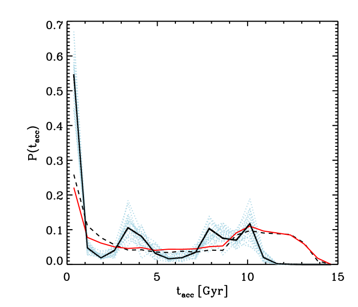
Figure 3.— Posterior distribution of satellite accretion times, from the MW satellite analogs (black), from hosts with exactly two subhalos (dashed), and from MW mass analogs (red). Selecting hosts with MC-like satellites strongly weights the distribution towards recent accretion. The blue-gray dotted lines show the distributions for 25 random MW satellite analogs drawn from our bootstrap analysis.

7. Conclusions

The advent of high-resolution cosmological simulations which sample the dynamical histories of large numbers of dark matter halos in a wide range of environments provides us with a new approach for determining the properties of individual halos given their observational characteristics. Here, we use the observed properties of the Magellanic Clouds to constrain the mass distribution and assembly history of the Milky Way. In comparison to previous efforts which use detailed observations but a necessarily simplified dynamical model, our approach uses simple observations and statistical inference from sampling of a detailed and cosmologically consistent dynamical model.

Our principal conclusions are:

1. We infer the MW halo mass to be ${\rm M}_{\rm MW}=1.2^{+0.7}_{-0.4}{\rm\,(stat.)}^{+0.3}_{-0.3}{\rm\,(sys.)}\times 10^{12}{\rm M}_{\odot}$ (68% confidence), in very good agreement with the recent stellar velocity measurements (Xue et al. 2008), with similarly sized error bars.

2. The MW halo has a slightly higher concentration than is typical for its mass: $11\pm 2$, compared to $8.7\pm 3.5$. Additionally, the density within 8 kpc is 60% higher for satellite analogs than for mass analogs.

3. Typical bright satellites of halos with MW mass were accreted at a range of epochs, generally at high redshift (c. 10 Gyr ago) or much more recently (within the last 2 Gyr). Because of their high speed near the center of the halo, we find a 72% probability that the Magellanic Clouds were accreted within the last Gyr. We also find a 50% probability that the MCs were accreted within 1 Gyr of each other.

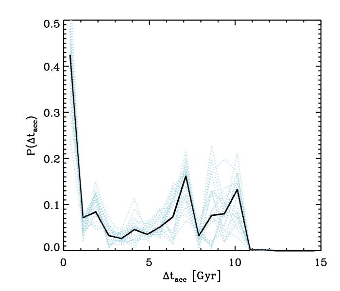
Figure 4.— Difference between accretion times for the two most massive satellites in MW-like systems. The solid line represents satellite analogs; the dashed line shows all systems with exactly two subhalos. The blue-gray dotted lines show the distributions for 25 random MW satellite analogs drawn from our bootstrap analysis.

This approach clearly allows one to explore a wide range of additional properties of MW-like halos; however, it places challenging requirements on the simulations used. In particular, for MW studies we are still limited by the relatively small simulation volume used. With the constraints used here, we found just one good fit halo per $\sim$ $500\rm{Mpc}^{3}$, emphasizing the large volume required to perform this analysis. As more criteria are applied we will need to sample a larger range of formation histories and environments drawn from a larger cosmological volume. In addition, the properties of its smaller satellites are not accessible with our present resolution. Pushing forward on both simulated resolution and volume will be essential to realize the full potential of this approach. Additionally, the simulations used here ignore the impact of baryons on the dark matter distribution. We have included a simple model of the stellar disk which is applied to the satellite velocities to get a handle on the impact of this systematic, but the model is simplistic and the effects of the baryonic component need to be further studied.

As we were completing this work, Boylan-Kolchin et al. (2010) presented results from a similar study. Their principal results regarding the mass of the MW and the accretion history of the LMC and SMC are in reasonable agreement with our own, although they favor a somewhat larger MW mass, $\hbox{$M_{\rm vir}$}\sim(2-3)\times 10^{12}\hbox{${\rm M}_{\odot}$}$. These studies differ in the 16 times larger volume simulation used here, the cosmology of the simulations, as well as our use of statistical inference. Boylan-Kolchin et al. (2010) used a simulation with cosmological parameters taken from the 1-year WMAP results, with $\Omega_{M}=0.25$, $\sigma_{8}=0.9$, and $h=0.73$, while the Bolshoi simulation uses the more recent WMAP7 results and features a lower $\sigma_{8}=0.82$, with $\Omega_{m}=0.27$ and $h=0.7$. Adopting the Tinker et al. (2008) mass function, we can understand the impact of these cosmological differences by considering the abundances of MW and MC mass objects. Differences come from a number of competing effects. First, due to cosmological differences, their lower $\sigma_{8}$ will tend to suppress our mass function, while the lower $h$ will increase the halo masses. In this case, the differences in $h$ has the more significant impact, and causes the abundances of halos with $\hbox{$M_{\rm vir}$}=1.2\times 10^{12}\hbox{${\rm M}_{\odot}$}$ to be suppressed by about 10% in the Millennium cosmology. However, the more relevant number is the ratio of the number density for our selected satellites to their selected hosts. Adopting the fiducial mass for the LMC, 100 times lower than that of the MW, we see that the ratio in number densities is $65.0$ in Bolshoi vs. $63.2$ in Millennium, a suppression of roughly $\sim 3\%$. Because the mass function is relatively flat here, reproducing the Bolshoi abundance ratio requires that the host mass increases to $3.6\times 10^{12}\hbox{${\rm M}_{\odot}$}$, a correction that brings our results into better agreement with theirs. However, it is also important to note that significantly different selection criteria for identifying “MW-like” objects were employed. Boylan-Kolchin et al. (2010) selected hosts whose two largest subhalos were within 0.75 $r_{\rm 200}$ and had similar total velocities and stellar masses to the MCs using abundance matching to estimate the stellar content of their simulated halos. In this work, we select objects with exactly two subhalos more massive than ${\rm v}_{\rm max}=50$km $s^{-1}$within a fixed 300 kpc aperture and then weight our sample according to how well the subhalos look like the MCs in terms of ${\rm v}_{\rm max}$, position, radial velocity, and total speed. These differences likely account for the tension in the resulting ${\rm M}_{\rm MW}$ PDFs. In particular, their focus on the total speed, $s$, of the magellanic clouds has likely biased their mass estimates for the MW high. This is shown by comparing the green and black lines in Figure 1, which show the likelihood distribution of masses for hosts having two satellites with similar speed to the MCs (green), as well as for hosts with two satellites with similar speeds, masses, and positions (black). The green distribution presents a much better agreement with Figure 13 of Boylan-Kolchin et al. (2010).

References

- Battaglia et al. (2005) Battaglia, G., et al. 2005, MNRAS, 364, 433
- Belokurov et al. (2007) Belokurov, V., et al. 2007, ApJ, 654, 897
- Besla et al. (2007) Besla, G., Kallivayalil, N., Hernquist, L., Robertson, B., Cox, T. J., van der Marel, R. P., & Alcock, C. 2007, ApJ, 668, 949
- Besla et al. (2010) Besla, G., Kallivayalil, N., Hernquist, L., van der Marel, R. P., Cox, T. J., & Kereš, D. 2010, ApJ, 721, L97
- Boylan-Kolchin et al. (2010) Boylan-Kolchin, M., Besla, G., & Hernquist, L. 2010, ArXiv e-prints
- Busha et al. (2007) Busha, M. T., Evrard, A. E., & Adams, F. C. 2007, ApJ, 665, 1
- Busha et al. (2010) Busha, M. T., Wechsler, R. H., & Behroozi, P. 2010, accepted to ApJ, arXiv:1011.6373
- Connors et al. (2006) Connors, T. W., Kawata, D., & Gibson, B. K. 2006, MNRAS, 371, 108
- Conroy et al. (2006) Conroy, C., Wechsler, R. H., & Kravtsov, A. V. 2006, ApJ, 647, 201
- Dehnen et al. (2006) Dehnen, W., McLaughlin, D. E., & Sachania, J. 2006, MNRAS, 369, 1688
- D’Onghia & Lake (2008) D’Onghia, E., & Lake, G. 2008, ApJ, 686, L61
- Gardiner et al. (1994) Gardiner, L. T., Sawa, T., & Fujimoto, M. 1994, MNRAS, 266, 567
- Gnedin et al. (2010) Gnedin, O. Y., Brown, W. R., Geller, M. J., & Kenyon, S. J. 2010, ApJ, 720, L108
- Harris & Zaritsky (2006) Harris, J., & Zaritsky, D. 2006, AJ, 131, 2514
- Kallivayalil et al. (2006a) Kallivayalil, N., van der Marel, R. P., & Alcock, C. 2006a, ApJ, 652, 1213
- Kallivayalil et al. (2006b) —. 2006b, ApJ, 652, 1213
- Kallivayalil et al. (2006c) Kallivayalil, N., van der Marel, R. P., Alcock, C., Axelrod, T., Cook, K. H., Drake, A. J., & Geha, M. 2006c, ApJ, 638, 772
- Klypin & Holtzman (1997) Klypin, A., & Holtzman, J. 1997, ArXiv Astrophysics e-prints
- Klypin et al. (2010) Klypin, A., Trujillo-Gomez, S., & Primack, J. 2010, ArXiv e-prints
- Klypin et al. (2002) Klypin, A., Zhao, H., & Somerville, R. S. 2002, ApJ, 573, 597
- Kravtsov et al. (2004) Kravtsov, A. V., Berlind, A. A., Wechsler, R. H., Klypin, A. A., Gottlöber, S., Allgood, B., & Primack, J. R. 2004, ApJ, 609, 35
- Kravtsov et al. (1997) Kravtsov, A. V., Klypin, A. A., & Khokhlov, A. M. 1997, ApJS, 111, 73
- Kuhlen et al. (2010) Kuhlen, M., Weiner, N., Diemand, J., Madau, P., Moore, B., Potter, D., Stadel, J., & Zemp, M. 2010, JCAP, 2, 30
- Lewis & Bridle (2002) Lewis, A., & Bridle, S. 2002, Phys. Rev. D, 66, 103511
- Li & White (2008) Li, Y., & White, S. D. M. 2008, MNRAS, 384, 1459
- Lin & Lynden-Bell (1982) Lin, D. N. C. and Lynden-Bell, D. 1982, MNRAS, 198, 707
- Lisanti et al. (2010) Lisanti, M., Strigari, L. E., Wacker, J. G., & Wechsler, R. H. 2010, ArXiv e-prints
- Liu et al. (2010) Liu, L., Gerke, B., Wechsler, R., Behroozi, P., & Busha, M. 2011, ApJ, 733, 62
- MacKay (2003) MacKay, D. J. C. 2003, “Information Theory, Inference and Learning Algorithms”. Cambridge: CUP
- Murai & Fujimoto (1980) Murai, T., & Fujimoto, M. 1980, PASJ, 32, 581
- Neal (2001) Neal, R. M. 2001, Statistics and Computing, 11, 125
- Piatek et al. (2008) Piatek, S., Pryor, C., & Olszewski, E. W. 2008, AJ, 135, 1024
- Smith et al. (2007) Smith, M. C., et al. 2007, MNRAS, 379, 755
- Stanimirović et al. (2004) Stanimirović, S., Staveley-Smith, L., & Jones, P. A. 2004, ApJ, 604, 176
- Strigari et al. (2007) Strigari, L. E., Bullock, J. S., Kaplinghat, M., Diemand, J., Kuhlen, M., & Madau, P. 2007, ApJ, 669, 676
- Strigari & Trotta (2009) Strigari, L. E., & Trotta, R. 2009, Journal of Cosmology and Particle Physics, 11, 19
- Suyu et al. (2010) Suyu, S. H., Marshall, P. J., Auger, M. W., Hilbert, S., Blandford, R. D., Koopmans, L. V. E., Fassnacht, C. D., & Treu, T. 2010, ApJ, 711, 201
- Tinker et al. (2008) Tinker, J., Kravtsov, A. V., Klypin, A., Abazajian, K., Warren, M., Yepes, G., Gottlöber, S., & Holz, D. E., ApJ, 688, 709
- Tollerud et al. (2008) Tollerud, E. J., Bullock, J. S., Strigari, L. E., & Willman, B. 2008, ApJ, 688, 277
- Tollerud et al. (2011) Tollerud, E. J., Boylan-Kolchin, M., Barton, E. S., Bullock, & Trinh, C. Q. 2011, arXiv:1103.1875
- Trujillo-Gomez et al. (2010) Trujillo-Gomez, S., Klypin, A., Primack, J., & Romanowsky, A. J. 2010, ArXiv e-prints, arXiv:1005.1289
- van den Bergh (2000) van den Bergh, S. 2000, The Galaxies of the Local Group, ed. van den Bergh, S. (Cambridge)
- van der Marel et al. (2002) van der Marel, R. P., Alves, D. R., Hardy, E., & Suntzeff, N. B. 2002, AJ, 124, 2639
- Vogelsberger et al. (2009) Vogelsberger, M., et al. 2009, MNRAS, 395, 797
- Walsh et al. (2009) Walsh, S. M., Willman, B., & Jerjen, H. 2009, AJ, 137, 450
- Watkins et al. (2010) Watkins, L. L., Evans, N. W., & An, J. H. 2010, MNRAS, 406, 264
- Wechsler et al. (2002) Wechsler, R. H., Bullock, J. S., Primack, J. R., Kravtsov, A. V., & Dekel, A. 2002, ApJ, 568, 52
- Xue et al. (2008) Xue, X. X., et al. 2008, ApJ, 684, 1143