Degrees of Freedom Regions of Two-User MIMO Z and Full Interference Channels: The Benefit of Reconfigurable Antennas

Abstract

We study the degrees of freedom (DoF) regions of two-user multiple-input multiple-output (MIMO) Z and full interference channels in this paper. We assume that the receivers always have perfect channel state information. We first derive the DoF region of Z interference channel with channel state information at transmitter (CSIT). For full interference channel without CSIT, the DoF region has been fully characterized recently and it is shown that the previously known outer bound is not achievable. In this work, we investigate the no-CSIT case further by assuming that the transmitter has the ability of antenna mode switching. We obtain the DoF region as a function of the number of available antenna modes and reveal the incremental gain in DoF that each extra antenna mode can bring. It is shown that in certain cases the reconfigurable antennas can bring extra DoF gains. In these cases, the DoF region is maximized when the number of modes is at least equal to the number of receive antennas at the corresponding receiver, in which case the previously outer bound is achieved. In all cases, we propose systematic constructions of the beamforming and nulling matrices for achieving the DoF region. The constructions bear an interesting space-frequency interpretation.

I Introduction

Characterizing the capacity region of interference channel has been a long open problem. Many researchers investigated this important problem, and the capacity regions of certain interference channels are known when the interference is strong, e.g. [1, 2, 3]. However, when the interference is not strong, the capacity region is still unknown. Recent progress reveals the capacity region for two-user interference channel to within one bit [4], and after that the sum capacity for very weak interference channel is settled [5, 6, 7]. Recently, a deterministic channel model has been proposed and used to explore the capacity of Gaussian interference network [8, 9, 10] such that the gap to capacity region can be bounded up to a constant value.

When it comes to multiple-input multiple-output (MIMO) networks, the capacity regions of certain MIMO interference channels are known [11, 12]. Instead of trying to characterize the capacity region completely, the degrees of freedom (DoF) region characterizes how capacity scales with transmit power as the signal-to-noise ratio goes to infinity.

It is well-known that in certain cases, the absence of channel state information at transmitter (CSIT) will not affect the DoF for MIMO networks, e.g., in the multiple access channel [13]. In other cases, CSIT does play an important role. For example, using interference alignment scheme, it is shown that the total DoF of a $K$-user MIMO interference channel is $MK/2$, where $M$ is the number of antennas of each user [14]. The key idea is to pack interferences from multiple sources so as to reduce the dimensionality of signal space spanned by interference.

The DoF region of two-user MIMO interference channel with CSIT has been obtained in [15], where it is shown that zero forcing is enough to achieve the DoF region. However, it is a different story in two-user MIMO X channel, where each transmitter has a message to every receiver. In [16] it is shown that interference alignment is the key to achieving the DoF region of MIMO X network. The DoF region of two-user MIMO broadcast channel and interference channel without CSIT are considered in [17], where there is an uneven trade-off between the two users. Except for a special case, the DoF region for the interference channel is known and achievable. Similar, but more general result of isotropic fading channel can be found in [18]. The DoF regions of the $K$-user MIMO broadcast, interference and cognitive radio channels are derived in [19] for some cases. However, the special case in [17] remains unsolved.

When only one of the two transmitter-receiver pairs is subject to interference, the interference channel is termed as Z interference channel (ZIC). To avoid confusion, we will call the channel where both pairs are subject to interference the full interference channel (FIC). The capacity region of MIMO Gaussian ZIC is established in [20] under very strong interference and aligned strong interference assumptions. In [21], the authors considered the capacity region of a single antenna ZIC without CSIT using deterministic approach.

Recently, it is shown in [22] that if the channel is staggered block fading, we can explore the channel correlation structure to do interference alignment, where the upper bound in the converse can be achieved in some special cases. For example, it is shown that for two-user MIMO staggered block fading FIC with 1 and 3 antennas at transmitters, 2 and 4 antennas at their corresponding receivers and without CSIT, the DoF pair $(1,1.5)$ can be achieved. The idea was further clarified in [23], where a blind interference alignment scheme is also proposed for $K$-user multiple-input single-output (MISO) broadcast channel to achieve DoF outer bound when CSIT is absent. Also recently, it is shown in [24] that the previous outer bound is not tight when the channels are independent and identical distributed (i.i.d.) over time and isotropic over spatial domain. So by now the DoF region of two-user MIMO FIC is completely known for both the case with CSIT and the no CSIT case (receiver-side CSI, or CSIR, is always assumed available), provided that the channel is i.i.d. over time and isotropic over spatial domain. However, when the channel is not i.i.d. over time such as in the “staggered” fading channels [22], the DoF could be larger.

In this paper, we consider the ZIC channel with CSIT, and both ZIC and FIC without CSIT but with reconfigurable antennas. Specifically, we obtain the DoF regions for the cases of:

1. ZIC with CSIT. We show that zero forcing is sufficient for achieving the DoF region in this case (Theorem 1).

2. ZIC and FIC when transmitter one has the number $K$ of antennas modes at least equal to $N_{1}$ (Theorems 2 and 3). Increasing $K$ beyond $N_{1}$ does not bring more gains in DoF.

3. ZIC and FIC when $M_{1}\leq K<N_{1}$, in which case each additional antenna mode brings an incremental gain on the DoF region (Theorem 4).

We present joint beamforming and nulling schemes to achieve the DoF region in all cases. When reconfigurable antennas are used, our proposed schemes have an interesting space-frequency coding explanation.

The rest of the paper is organized as follows. We first present the system model in Section II. Known results on the DoF region of two-user MIMO FIC are also briefly reviewed. The DoF region of ZIC with CSIT is discussed in Section III. The DoF regions of ZIC and FIC without CSIT when there are enough antenna modes are investigated in Section IV. When there are not enough modes, the DoF region is given in Section V. Finally, Section VI concludes this paper.

Notation: boldface uppercase (lowercase) letters denote matrices (vectors). $\mathbb{R},\mathbb{Z},\mathbb{C}$ are the real, integer and complex numbers sets. $\mathcal{CN}(0,1)$ denotes a circularly symmetric complex Gaussian (CSCG) distribution with zero mean and unit variance. We use $\boldsymbol{A}\otimes\boldsymbol{B}$ to denote the Kronecker product between $\boldsymbol{A}$ and $\boldsymbol{B}$. $\boldsymbol{0}$ and $\boldsymbol{1}$ denote all one and all zero matrices (vectors), respectively. $\boldsymbol{A}^{T}$ and $\boldsymbol{A}^{\dagger}$ denote the transpose and Hermitian of $\boldsymbol{A}$, respectively. We also use notation like $\boldsymbol{A}_{m\times n}$ to emphasize that $\boldsymbol{A}$ is of size $m\times n$. We use $\boldsymbol{I}_{m}$ to denote a size $m\times m$ identity matrix and $\boldsymbol{1}_{m}$ to denote an all-one column vector with length $m$. Denote $\boldsymbol{g}_{n}(a):=[1,a,a^{2},\dots,a^{n-1}]^{T}$. A size $n\times m$ Vandermonde matrix based on a set of element $\{a_{1},a_{2},\dots,a_{m}\}$ is defined as $\boldsymbol{\mathcal{V}}_{n}(a_{1},a_{2},\dots,a_{m})=[\boldsymbol{g}_{n}(a_{1}),\boldsymbol{g}_{n}(a_{2}),\dots,\boldsymbol{g}_{n}(a_{m})]$. We use $\mathcal{I}(\boldsymbol{x};\boldsymbol{y})$ to denote the mutual information between $\boldsymbol{x}$ and $\boldsymbol{y}$. The differential entropy of a continuous random variable $\boldsymbol{x}$ is denoted as $\mathcal{H}(\boldsymbol{x})$.

II System Model and Known Results

II-A Channel Model

Consider a MIMO interference channel with two transmitters and two receivers, the number of transmit (receive) antennas at the $i$th transmitter (receiver) is denoted as $M_{i}$ ($N_{i}$), $i\in\{1,2\}$. The system is termed as an ($M_{1},N_{1},M_{2},N_{2}$) system, which can be described as

$$\boldsymbol{y}_{1}(t)=\boldsymbol{H}_{11}(t)\boldsymbol{x}_{1}(t)+\boldsymbol{H}_{12}(t)\boldsymbol{x}_{2}(t)+\boldsymbol{z}_{1}(t)$$ (1)

$$\boldsymbol{y}_{2}(t)=\boldsymbol{H}_{21}(t)\boldsymbol{x}_{1}(t)+\boldsymbol{H}_{22}(t)\boldsymbol{x}_{2}(t)+\boldsymbol{z}_{2}(t)$$ (2)

where $t$ is the time index, $\boldsymbol{y}_{i}(t)\in\mathbb{C}^{N_{i}}$, $\boldsymbol{z}_{i}(t)\in\mathbb{C}^{N_{i}}$ are the received signal and additive noise of receiver $i$, respectively. The entries of $\boldsymbol{z}_{i}(t)$ are independent and identically $\mathcal{CN}(0,1)$ distributed in both time and space. The channel between the $i$th transmitter and the $j$th receiver is denoted as $\boldsymbol{H}_{ji}(t)\in\mathbb{C}^{N_{j}\times M_{i}}$. We assume the probability of $\boldsymbol{H}_{ji}(t)$ belonging to any subset of $\mathbb{C}^{N_{j}\times M_{i}}$ that has zero Lebesgue measure is zero. For the two-user MIMO ZIC, $\boldsymbol{H}_{21}(t)=0$. $\boldsymbol{x}_{i}(t)\in\mathbb{C}^{M_{i}}$ is the input signal at transmitter $i$ and $\boldsymbol{x}_{1}(t)$ is independent of $\boldsymbol{x}_{2}(t)$. The transmitted signals satisfy the following power constraint:

$$\text{E}(||\boldsymbol{x}_{i}(t)||^{2})\leq P\quad i=1,2.$$ (3)

Denote the capacity region of the two-user MIMO system as $C(P)$, which contains all the rate pairs $(R_{1},R_{2})$ such that the corresponding probability of error can approach zero as coding length increases. The DoF region is defined as follows [17]

$$\mathcal{D}:=\left\{(d_{1},d_{2})\in\mathbb{R}^{+}_{2}:\exists(R_{1}(P),R_{2}(P))\in C(P),\right.\left.\text{such that }d_{i}=\lim_{P\to\infty}\frac{R_{i}(P)}{\log(P)},\quad i=1,2\right\}.$$

II-B Reconfigurable antennas

Assume the CSI at receiver (CSIR) is always available. We would like to study the DoF regions of MIMO FIC and ZIC with or without CSIT under an additional assumption that one transmitter is equipped with reconfigurable antennas. The reconfigurable antennas are different from the conventional antennas as they can be switched to different pre-determined modes so that the channel fluctuation can be introduced artificially. Similar to [23], we use reconfigurable antennas to explore multiplexing gain other than diversity gain.

We assume that only one transmitter is equipped with reconfigurable antennas. We define one antenna mode as one possible configuration of a single transmit antenna such that by switching to a different mode, the channel between this transmit antenna and all receive antennas is changed. Different antenna modes can be realized via spatially separated physical antennas, or the same physical antenna excited with different polarizations, and so on. The benefit of antenna mode switching lies in the fact that channel variation can be artificially created, without the need to increase the number of RF chains. We let $K$ denote the total number of antenna modes available at the transmitter with reconfigurable antennas (usually transmitter one).

We make the following assumption of the channel in this paper: the channel is block fading with coherent length of $L$ symbols. Within each coherent block, the channels between all the transmitter modes and the receive antennas remain constant. The channels between the $K$ modes of the reconfigurable transmitter and both receivers are isotropic, in the sense of [24]. From block to block, the channel changes independently.

When $K>M$, the transmitter has the freedom to use different modes at different slots. For a given antenna mode usage pattern over the length of a whole coherent block, the effective channel for the whole block is not isotropic fading and not i.i.d. over the time slots within the block.

One may view our model approximately as a transition from an effective channel where all the links have exactly the same coherent time as in [24] to an effective channel where the links do not have the same coherent time [22]. However, there are two important distinctions between antenna mode switching and variation of channel coherence time: i) Antenna switching can be initiated at will at the transmitter, whereas channel coherence structure is in general not controllable. ii) The resulting equivalent channel from antenna mode switching is not “staggered” [22], so methods therein do not apply here.

II-C Known Results on FIC

We first present some known results on DoF region of MIMO full interference channel which will be useful for developing our results.

The total degrees of freedom of two-user MIMO full interference channel with CSIT is developed in [15, Theorem 2], which leads to the following DoF regions:

$$d_{i} \leq\min(M_{i},N_{i}),\quad i=1,2;$$ (4)

$$d_{1}+d_{2} \leq\min(\max(N_{1},M_{2}),\max(M_{1},N_{2}),N_{1}+N_{2},M_{1}+M_{2}).$$ (5)

An outer bound of degrees of freedom region of two-user MIMO full interference channel without CSIT is as follows [18, Theorem 1]:

$$d_{i}\leq\min(M_{i},N_{i}),\quad i=1,2;$$ (6)

$$d_{1}\!+\!\frac{\min(N_{1},N_{2},M_{2})}{\min(N_{2},M_{2})}d_{2}\leq\min(M_{1}+M_{2},N_{1});$$ (7)

$$\frac{\min(N_{1},N_{2},M_{1})}{\min(N_{1},M_{1})}d_{1}\!+\!d_{2}\leq\min(M_{1}+M_{2},N_{2}).$$ (8)

Note that the same result is also given in [17], though in a less compact form.

It is shown in [17] that the outer bound given in (6)–(8) can be achieved by zero forcing or time sharing except for the case $M_{1}<N_{1}<\min(M_{2},N_{2})$, for which it was not known how to achieve

$$(d_{1},d_{2})=\left(M_{1},\frac{\min(M_{2},N_{2})(N_{1}-M_{1})}{N_{1}}\right)$$ (9)

in general. The cases when $N_{1}>N_{2}$ can be converted by switching the user indices. It is shown in [24] that when the channel is isotropic fading and i.i.d. over time, the outer bound given in (6)–(8) is not tight: if $N_{1}\leq N_{2}$, the DoF region of FIC without CSIT can be given as follows:

$$d_{i}\leq\min(M_{i},N_{i}),\quad i=1,2;$$ (10)

$$d_{1}\!+\!\frac{\min(N_{1},M_{2})-\alpha}{\min(N_{2},M_{2})-\alpha}(d_{2}-\alpha)\leq\min(M_{1},N_{1}).$$ (11)

where $\alpha=\min(M_{1}+M_{2},N_{1})-\min(M_{1},N_{1})$. In other words, (9) is not achievable when $M_{1}<N_{1}<\min(M_{2},N_{2})$, as (11) is reduced to

$$d_{1}+\frac{M_{1}}{\min(M_{2},N_{2})-(N_{1}-M_{1})}d_{2} \leq M_{1}+\frac{M_{1}(N_{1}-M_{1})}{\min(M_{2},N_{2})-(N_{1}-M_{1})}$$ (12)

and the DoF pair $(d_{1},d_{2})=(M_{1},N_{1}-M_{1})$ is on the boundary of the DoF region.

III Two-User MIMO ZIC with CSIT

In this section, we prove the following theorem.

Theorem 1 (ZIC with CSIT)

The DoF region of a two-user MIMO Z interference channel with CSIT is described by

$$d_{i} \leq\min(M_{i},N_{i}),\quad i=1,2;$$ (13)

$$d_{1}+d_{2} \leq\min(\max(N_{1},M_{2}),N_{1}+N_{2},M_{1}+M_{2}).$$ (14)

Proof:

We split the proof into the achievability and converse parts, as the following two lemmas. The theorem can be proved by showing the regions given by Lemma 1 and Lemma 2 are the same for all the cases.  

Lemma 1 (Achievability part of Theorem 1)

The following region of two-user MIMO ZIC with CSIT is achievable:

$$d_{i} \leq\min(M_{i},N_{i}),\quad i=1,2;$$ (15)

$$d_{1}+d_{2} \leq\min(N_{1},M_{1}+\min(N_{2},M_{2}))1({M_{2}<N_{1}})$$

$$+\min(M_{2},N_{2}+\min(N_{1},M_{1}))1({M_{2}\geq N_{1}})$$ (16)

where $1(\cdot)$ is indicator function.

Proof:

If $M_{2}\geq N_{1}$ and assume transmitter 1 sends $d_{1}$ streams, transmitter 2 can send at most $M_{2}-N_{1}$ streams along the null space of $\boldsymbol{H}_{12}$ without interfering receiver 1. Transmitter 2 can also send at most $N_{1}-d_{1}$ streams along the row space of $\boldsymbol{H}_{12}$. Therefore user 2 can decode $\min((M_{2}-N_{1})+(N_{1}-d_{1}),N_{2})$ streams without interfering receiver 1. If $N_{1}\geq M_{2}$ and assume transmitter 2 sends $d_{2}$ streams which interfere receiver 1, transmitter 1 can send $\min(N_{1}-d_{2},M_{1})$ decodable streams to receiver 1. Combining these two cases, we have the achievable DoF region shown in this lemma.  

Lemma 2 (Conversepart of Theorem 1)

The region given by (13) and (14) is a valid outer bound for the two-user MIMO ZIC with CSIT.

Proof:

It is obvious that adding antennas at the receiver will not shrink the DoF region. Hence, we can add $M_{1}$ antennas to receiver 2 resulting an $(M_{1},N_{1},M_{2},M_{1}+N_{2})$ MIMO FIC, and (14) follows from Corollary 1 in [15]. The outer bound of such a MIMO FIC is a valid outer bound of an $(M_{1},N_{1},M_{2},N_{2})$ MIMO ZIC. Combining the trivial upper bound on point-to-point system, we have this lemma.  

Based on Lemma 1, zero forcing at receiver is sufficient to achieve the DoF region of ZIC when CSIT is available. The antenna mode switching ability is not needed in this case. However, we shall see later that such an ability is important for the case when CSIT is absent.

IV Two-User MIMO ZIC and FIC without CSIT When Number of Modes $K\geq N_{1}$

In this section, we describe the DoF region of two-user ZIC and FIC without CSIT but with transmitter side reconfigurable antennas. We deal with the case that $K$, the number of antenna modes is at least equal to the $N_{1}$. The case $K<N_{1}$ will be dealt with in Section V.

Based on the antenna number configuration, the achievability scheme of ZIC and FIC without CSIT can be divided into two cases. In the first case, no reconfigurable antenna is needed to achieve an DoF outer bound — reconfigurable antennas are not helpful (Section IV-B). In the second case, the outer bound can be achieved with enough transmit side antenna modes (Section IV-C): reconfigurable antennas enlarges the DoF region. Our main results in this section are the following two theorems.

Theorem 2 (ZIC with Enough Reconfigurable Antenna Modes)

The DoF region of two-user MIMO Z interference channel without CSIT is described by the following inequalities

$$d_{i}\leq\min(M_{i},N_{i}),\quad i=1,2;$$ (17)

$$d_{1}\!+\!\frac{\min(N_{1},N_{2},M_{2})}{\min(N_{2},M_{2})}d_{2}\!\leq\!\min(M_{1}\!+M_{2},N_{1}).$$ (18)

if either one of the following is true:

1. $M_{1}<N_{1}<\min(M_{2},N_{2})$ and transmitter one can switch among $N_{1}$ antenna modes, or

2. $(M_{1},N_{1},M_{2},N_{2})$ do not satisfy the above condition.  

The DoF region in Theorem 2 is shown in Fig. 1.

Theorem 3 (FIC with Enough Reconfigurable Antenna Modes)

The DoF region of two-user MIMO full interference channel without CSIT is described by the inequalities (6)–(8) if any one of the following is true:

1. $M_{1}<N_{1}<\min(M_{2},N_{2})$ and transmitter one can switch among $N_{1}$ antenna modes, or

2. $M_{2}<N_{2}<\min(M_{1},N_{1})$ and transmitter two can switch among $N_{2}$ antenna modes, or

3. $(M_{1},N_{1},M_{2},N_{2})$ are not one of the two above cases.  

IV-A Converse part

We first prove the converse part of the two theorems.

Lemma 3 (Converse part of Theorem 3)

The outer bound of DoF region of two-user MIMO full interference channel given in (6)–(8) is still valid when either or both transmitters are using antenna mode switching.

Proof:

The outer bound (7) has been derived based on the assumption that the rows of $\boldsymbol{H}_{12}$ and those of $\boldsymbol{H}_{22}$ are statistically equivalent [17, 18]. Similarly, the outer bound (8) has been derived based on the assumption that the rows of $\boldsymbol{H}_{11}$ and those of $\boldsymbol{H}_{21}$ are statistically equivalent. These assumptions are not affected by antenna mode switching at either or both transmitters. Hence, the DoF outer bound is still valid.  

Lemma 4 (Converse part of Theorem 2)

The outer bound of degrees of freedom region of two-user MIMO Z interference channel without CSIT can be given as when transmitter one has the antenna mode switching ability

$$d_{i}\leq\min(M_{i},N_{i}),\quad i=1,2;$$ (19)

$$d_{1}\!+\!\frac{\min(N_{1},N_{2},M_{2})}{\min(N_{2},M_{2})}d_{2}\!\leq\!\min(M_{1}\!+M_{2},N_{1}).$$ (20)

Proof:

This is the direct result of [18, Theorem 1] as in (6)–(8), by noticing that there is no interference from transmitter 1 to receiver 2 hence (8) is not longer needed. The antenna switching at transmitter one does not affect the upper bound, for the same reason stated in Lemma 3.  

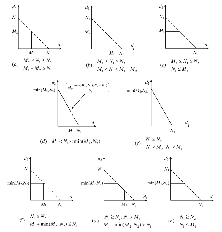
Figure 1: DoF region of two-user MIMO ZIC without CSIT when number of antenna modes $K\geq N_{1}$. Figures (a)–(e) are for the case $N_{1}\leq N_{2}$; Figures (f)–(h) are for the case $N_{1}\geq N_{2}$.

IV-B Achievability: when antenna mode switching is not needed

In this section, we prove the achievability part for Case C2) of Theorem 2 and Case C3) of Theorem 3. Achievability for the remaining cases are left to Section IV-C.

Lemma 5

For the two-user MIMO Z interference channel without CSIT, when $N_{1}\geq N_{2}$, (20) is achievable by zero forcing.

Proof:

When $N_{1}\geq N_{2}$, the corresponding outer regions are shown in Fig. 1 (f)–(h). Noticing that (20) is reduced to $d_{1}+d_{2}\leq\min(M_{1}+M_{2},N_{1})$, zero forcing is sufficient to achieve the outer bound.  

Lemma 6

When CSIT is absent, the DoF outer region given by Lemma 4 of a two-user MIMO $(M_{1},N_{1},M_{2},N_{2})$ ZIC is the same as that of an $(M_{1},N_{1},\min(M_{2},N_{2}),\min(M_{2},N_{2}))$ ZIC.

Proof:

We give the proof case by case. It is trivial that when $M_{2}\leq N_{2}$ reducing the number of antennas at receiver 2 to $M_{2}$ will not shrink the DoF region. When $M_{2}>N_{2}$, we can further consider two sub-cases: $N_{2}\geq N_{1}$ and $N_{2}<N_{1}$.

1. When $M_{2}>N_{2}\geq N_{1}$, corresponding to Fig. 1 (d) and (e), the DoF bound (20) becomes $\frac{d_{1}}{N_{1}}+\frac{d_{2}}{N_{2}}\leq 1$. Hence the DoF outer region is the same as an $(M_{1},N_{1},N_{2},N_{2})$ ZIC.

2. When $M_{2}>N_{2}$ and $N_{2}<N_{1}$, the DoF bound (20) becomes $d_{1}+d_{2}\leq\min(M_{1}+M_{2},N_{1})$. Hence, if $M_{1}\geq N_{1}-N_{2}$, which implies $M_{1}+\min(M_{2},N_{2})\geq N_{1}$, the DoF outer region is a pentagon or a tetragon; see Fig. 1 (g) and (h). Otherwise, it is a square, see Fig. 1 (f). One can show that the region is the same as that of an $(M_{1},N_{1},N_{2},N_{2})$ ZIC.

Hence, the lemma holds.  

We also have the following lemma regarding the relationship between DoF regions of ZIC and FIC.

Lemma 7

When $N_{1}\leq N_{2}$, the MIMO ZIC and FIC have the same DoF regions. Any encoding scheme that is DoF optimal for one channel is also DoF optimal for the other.

Proof:

Any point in the FIC is also trivially achievable in the ZIC because user 2’s channel is interference free. Conversely, any point achievable in the ZIC region, is also achievable in FIC. This is based on the fact that the channels are statistically equivalent at both receivers. If receiver 1 can decode user 1’s message, then receiver 2, having at least as many antennas, must also be able to decode the same message. Receiver 2 can then subtract the decoded message, which renders the resulting channel the same as in the ZIC.  

Due to Lemma 7, we can translate all achievability schemes from FIC to ZIC and vice versa when $N_{1}\leq N_{2}$. Therefore the achievability schemes in [17] for FIC when $N_{1}\leq N_{2}$ and $M_{1}\geq N_{1}$ can be used for ZIC. Therefore, the achievability part for Case C2) of Theorem 2 is complete.

For the FIC, the achievability for the case $N_{1}\leq N_{2}$, except when $M_{1}<N_{1}<\min(M_{2},N_{2})$, is shown in [17]. When $N_{1}\geq N_{2}$, we can swap the indices of the two users, so that except for the Cases C1) and C2) the achievability scheme is known for FIC.

IV-C Achievability: with antenna mode switching when $K\geq M_{1}N_{1}$

In this subsection, we prove a weaker version of the achievability for Case C1) of Theorem 2 and Cases C1) and C2) of Theorem 3. Namely, we assume that the number of antenna modes available is $K\geq M_{1}N_{1}$. The scheme is simpler in this case, and the achievability scheme for the case $K=N_{1}$ will be built upon this case.

Based on Lemma 6 and Lemma 7, we only consider the two-user MIMO ZIC with $M_{1}<N_{1}<M_{2}=N_{2}$ to prove the Cases C1) for both theorems. Case C2) of Theorem 3 is the Case of C1) with user indices swapped. Therefore, we want to show that the following DoF pair is achievable for ZIC with $K_{1}=M_{1}N_{1}$ modes:

$$(d_{1},d_{2})=\left(M_{1},\frac{M_{2}(N_{1}-M_{1})}{N_{1}}\right).$$ (21)

We first notice that this point cannot be achieved by zero forcing over one time instant. This is because using zero forcing if transmitter 1 sends $M_{1}$ streams, transmitter 2 can only send $N_{1}-M_{1}$ streams without interfering receiver 1. If transmitter 2 sends more streams, the desired signal and interference are not separable at receiver 1 as transmitter 2 does not know channel state information so it cannot send streams along the null space of $\boldsymbol{H}_{12}$. A simple example is the $(1,2,3,3)$ case, where the outer bound gives us $(d_{1},d_{2})=(1,1.5)$, which is not achievable via zero forcing over one time slot. We make the assumption that the channel $\boldsymbol{H}_{12}$ stays the same for at least $N_{1}$ time slots. It is sufficient to show that $(M_{1}N_{1},M_{2}(N_{1}-M_{1}))$ streams can be achieved in $N_{1}$ time slots.

We first develop the beamforming and nulling design by assuming that there are $N_{1}M_{1}$ antenna modes available at transmitter 1 such that it can use different antenna modes in different slots to create channel variation. We will further show that the resultant beamforming and nulling design still work even if there are only $N_{1}$ modes available.

Here and after, we use tilde notation to indicate the time expansion signals, where the number of slots of time expansion signals shall be clear within the context. The time expansion channel between transmitter 1 and receiver 1 in $N_{1}$ time slots is

$$\tilde{\boldsymbol{H}}_{11}\!\!=\!\!\left[\!\begin{array}[]{ccccc}\!\boldsymbol{H}_{11}(1)&\boldsymbol{0}&\boldsymbol{0}&\boldsymbol{0}\\ \boldsymbol{0}&\!\boldsymbol{H}_{11}(2)&\boldsymbol{0}&\boldsymbol{0}\\ \vdots&\vdots&\ddots&\vdots\\ \boldsymbol{0}&\boldsymbol{0}&\boldsymbol{0}&\!\boldsymbol{H}_{11}(N_{1})\!\\ \end{array}\right]_{\!N_{1}^{2}\!\times\!N_{1}M_{1}}$$ (26)

and the channel between transmitter 2 and receiver 1 is

$$\tilde{\boldsymbol{H}}_{12}=\boldsymbol{I}_{N_{1}}\otimes\boldsymbol{H}_{12}(1)$$ (27)

as transmitter 2 does not create channel variation. We will use precoding at transmitter 2 only and nulling at receiver 1 only. Let $\tilde{\boldsymbol{P}}$ be the transmit beamforming matrix at transmitter 2 and $\tilde{\boldsymbol{Q}}$ be the nulling matrix at receiver 1. We propose to use the following structures for them

$$\tilde{\boldsymbol{P}}_{M_{2}N_{1}\times M_{2}(N_{1}-M_{1})} =\boldsymbol{P}_{N_{1}\times(N_{1}-M_{1})}\otimes\boldsymbol{I}_{M_{2}}$$ (28)

$$\tilde{\boldsymbol{Q}}_{M_{1}N_{1}\times N_{1}^{2}} =\boldsymbol{Q}_{M_{1}\times N_{1}}\otimes\boldsymbol{I}_{N_{1}}.$$ (29)

The received signal at receiver 1 can be written as

$$\tilde{\boldsymbol{y}}_{1}=\tilde{\boldsymbol{H}}_{11}\tilde{\boldsymbol{x}}_{1}+\tilde{\boldsymbol{H}}_{12}\tilde{\boldsymbol{P}}\tilde{\boldsymbol{x}}_{2}+\tilde{\boldsymbol{z}}_{1}$$ (30)

where $\tilde{\boldsymbol{x}}_{1}$ is a length $M_{1}N_{1}$ vector, and $\tilde{\boldsymbol{x}}_{2}$ is a length $M_{2}(N_{1}-M_{1})$ vector. After applying nulling matrix $\tilde{\boldsymbol{Q}}$, we have

$$\tilde{\boldsymbol{Q}}\tilde{\boldsymbol{y}}_{1}=\underbrace{\tilde{\boldsymbol{Q}}\tilde{\boldsymbol{H}}_{11}}_{\tilde{\boldsymbol{A}}}\tilde{\boldsymbol{x}}_{1}+\underbrace{\tilde{\boldsymbol{Q}}\tilde{\boldsymbol{H}}_{12}\tilde{\boldsymbol{P}}}_{\tilde{\boldsymbol{B}}}\tilde{\boldsymbol{x}}_{2}+\tilde{\boldsymbol{Q}}\tilde{\boldsymbol{z}}_{1}.$$ (31)

To achieve the degrees of freedom $(M_{1}N_{1},M_{2}(N_{1}-M_{1}))$ for both users, it is sufficient to design our $\tilde{\boldsymbol{P}}$ and $\tilde{\boldsymbol{Q}}$ to satisfy the following conditions simultaneously

1. $\text{rank}(\tilde{\boldsymbol{A}})=M_{1}N_{1}$,

2. $\text{rank}(\tilde{\boldsymbol{P}})=M_{2}(N_{1}-M_{1})$,

3. $\tilde{\boldsymbol{B}}=\boldsymbol{0}$.

The second condition can be easily satisfied. Because $\text{rank}(\tilde{\boldsymbol{P}})=\text{rank}(\boldsymbol{P})\text{rank}(\boldsymbol{I}_{M_{2}})$, we only need to design $\boldsymbol{P}$ such that $\text{rank}(\boldsymbol{P})=N_{1}-M_{1}$. As to the third condition, notice that

$$\tilde{\boldsymbol{B}} =(\boldsymbol{Q}\otimes\boldsymbol{I}_{N_{1}})(\boldsymbol{I}_{N_{1}}\otimes\boldsymbol{H}_{12}(1))(\boldsymbol{P}\otimes\boldsymbol{I}_{M_{2}})$$

$$=(\boldsymbol{Q}\boldsymbol{I}_{N_{1}}\boldsymbol{P})\otimes(\boldsymbol{I}_{N_{1}}\boldsymbol{H}_{12}(1)\boldsymbol{I}_{M_{2}})$$

$$=(\boldsymbol{Q}\boldsymbol{P})\otimes\boldsymbol{H}_{12}(1).$$

It is therefore sufficient (and also necessary) to have $\boldsymbol{Q}\boldsymbol{P}=\boldsymbol{0}$. Then the key is to find a $\boldsymbol{Q}$ such that the equivalent channel of user 1 after nulling

$$\tilde{\boldsymbol{A}}=(\boldsymbol{Q}\otimes\boldsymbol{I}_{N_{1}})\tilde{\boldsymbol{H}}_{11}$$ (32)

has full rank $M_{1}N_{1}$ with probability 1. The matrix $\tilde{\boldsymbol{A}}$ is of size ${M_{1}N_{1}\times M_{1}N_{1}}$ and has the following structure

$$\!\!\!\tilde{\boldsymbol{A}}\!\!=\!\!\left[\begin{array}[]{ccccc}\!\!\!q_{11}\boldsymbol{H}_{11}(1)\!\!\!&\!\!\!q_{12}\boldsymbol{H}_{11}(2)\!\!\!&\!\!\!\cdots&\!\!\!q_{1N_{1}}\boldsymbol{H}_{11}(N_{1})\!\!\!\\ \!\!\!q_{21}\boldsymbol{H}_{11}(1)\!\!\!&\!\!\!q_{12}\boldsymbol{H}_{11}(2)\!\!\!&\!\!\!\cdots&\!\!\!q_{2N_{1}}\boldsymbol{H}_{11}(N_{1})\!\!\!\\ \vdots&\vdots&\!\!\!\ddots&\vdots\\ \!\!\!q_{M_{1}1}\boldsymbol{H}_{11}(1)&\!\!\!q_{M_{1}2}\boldsymbol{H}_{11}(2)&\!\!\!\cdots&\!\!\!q_{M_{1}N_{1}}\boldsymbol{H}_{11}(N_{1})\!\!\!\end{array}\right].$$ (37)

To show that $\tilde{\boldsymbol{A}}$ has full rank, we need the following lemma, which is known before, and a proof of it can be found in e.g., [25].

Lemma 8

[25, Lemma 2] Consider an analytic function $h(\boldsymbol{x})$ of several variables $\boldsymbol{x}=[x_{1},\dots,x_{n}]^{T}\in\mathbb{C}^{n}$. If $h$ is nontrivial in the sense that there exists $\boldsymbol{x}_{0}\in\mathbb{C}^{n}$ such that $h(\boldsymbol{x}_{0})\neq 0$, then the zero set of $f(\boldsymbol{x})$ $\mathrm{Z}:=\{\boldsymbol{x}\in\mathbb{C}^{n}|h(\boldsymbol{x})=0\}$ is of measure (Lebesgue measure in $\mathbb{C}^{n}$) zero.  

Because the determinant of $\tilde{\boldsymbol{A}}$ is an analytic polynomial function of elements of $\boldsymbol{H}_{11}(t),t=1,\dots,N_{1}$, we only need to find a specific pair of $\boldsymbol{Q}$ and $\boldsymbol{H}_{11}(t),t=1,\dots,N_{1}$, such that $\tilde{\boldsymbol{A}}$ is full rank. We propose the following:

$$\boldsymbol{Q}=[\boldsymbol{\mathcal{V}}_{N_{1}}(1,\omega_{N_{1}},\dots,\omega^{M_{1}-1}_{N_{1}})]^{T},$$ (38)

where $\omega_{N_{1}}:=\exp(-j{2\pi}/{N_{1}})$.

Let $\omega:=\exp(-j{2\pi}/{N_{1}^{2}})$. Take the realizations of $\boldsymbol{H}_{11}(t)$, $t=1,\dots,N_{1}$, as

$$\boldsymbol{H}_{11}(t)=\boldsymbol{\mathcal{V}}_{N_{1}}(\omega^{t-1},\omega^{N_{1}+t-1},\dots,\omega^{(M_{1}-1)N_{1}+t-1}).$$ (39)

It can be verified that for such choices of $\boldsymbol{Q}$ and $\boldsymbol{H}_{11}(t)$, $\tilde{\boldsymbol{A}}$ is a Vandermonde matrix:

$$\tilde{\boldsymbol{A}}=\boldsymbol{\mathcal{V}}_{M_{1}N_{1}}(1,\omega^{N_{1}},\dots,\omega^{(M_{1}-1)N_{1}},\omega^{1},\omega^{N_{1}+1},\dots, \omega^{(M_{1}-1)N_{1}+1},$$

$$\dots,\omega^{N_{1}-1},\omega^{2N_{1}-1},\dots,\omega^{M_{1}N_{1}-1}),$$

hence of full rank. We also notice that $\tilde{\boldsymbol{A}}$ is a leading principal minor of a permuted fast Fourier transform (FFT) matrix with size $N_{1}^{2}\times N_{1}^{2}$. The permutation is as follows: Index the columns of an FFT matrix $0,1,\dots,N_{1}^{2}-1$, and then permute them in an order shown below:

$$(0,N_{1},2N_{1},\dots,(M_{1}-1)N_{1}),(1,N_{1}+1,2N_{1}+1,\dots,(M_{1}-1)N_{1}+1),...$$

Based on Lemma 8, if we choose the nulling matrix using $\boldsymbol{Q}$ as specified in (38), $\tilde{\boldsymbol{A}}$ has full rank almost surely. One choice of the corresponding $\boldsymbol{P}$ matrix with respect to (38) is the following

$$\boldsymbol{P}=\boldsymbol{\mathcal{V}}_{N_{1}}(\omega_{N_{1}}^{-M_{1}},\omega_{N_{1}}^{-(M_{1}+1)},\dots,\omega^{-(N_{1}-1)}_{N_{1}}),$$ (40)

which is orthogonal to $\boldsymbol{Q}$. This completes the achievability part under conditions in Case C1) of Theorem 2 and Cases C1) and C2) of Theorem 3, but with $K\geq M_{1}N_{1}$.

IV-D Achievability: with antenna mode switching when $K=N_{1}$

Assuming there are $N_{1}$ modes available at transmitter 1 and denote these channel vectors between receive antennas of user 1 and the $i$th mode as $\boldsymbol{h}_{i},1\leq i\leq N_{1}$ and let $\hat{\boldsymbol{H}}_{N_{1}\times N_{1}}=[\boldsymbol{h}_{1},\boldsymbol{h}_{2},\dots,\boldsymbol{h}_{N_{1}}]$. We choose the antenna modes to be switched cyclically:

$$\boldsymbol{H}_{11}(1) =[\boldsymbol{h}_{1},\boldsymbol{h}_{2},\dots,\boldsymbol{h}_{M_{1}}],$$ (41)

$$\boldsymbol{H}_{11}(2) =[\boldsymbol{h}_{2},\boldsymbol{h}_{3},\dots,\boldsymbol{h}_{M_{1}+1}],$$ (42)

$$\vdots$$

$$\boldsymbol{H}_{11}(N_{1}) =[\boldsymbol{h}_{N_{1}},\boldsymbol{h}_{1},\dots,\boldsymbol{h}_{M_{1}-1}].$$ (43)

We want to show that under this switching pattern, the equivalent channel $\tilde{\boldsymbol{A}}$ in (32) between transmitter one and receiver one after nulling, is still full rank. To show this, indexing the columns of $\tilde{\boldsymbol{A}}$ in (32) as $0,1,\dots,N_{1}M_{1}-1$, we then permute and group the columns of $\tilde{\boldsymbol{A}}$ in the following way:

$$(0,M_{1},2M_{1},\dots,(M_{1}-1)N_{1}),(1,M_{1}+1,2M_{1}+1,\dots,(M_{1}-1)N_{1}+1),...$$

Denote the permutation result as $\tilde{\boldsymbol{A}}^{\prime}$ and it can be expressed as

$$\tilde{\boldsymbol{A}}^{\prime}=\begin{bmatrix}\hat{\boldsymbol{H}}&\hat{\boldsymbol{H}}&\cdots&\hat{\boldsymbol{H}}\\ \boldsymbol{G}\hat{\boldsymbol{H}}&\omega_{N_{1}}^{-1}\boldsymbol{G}\hat{\boldsymbol{H}}&\cdots&\omega_{N_{1}}^{-M_{1}}\boldsymbol{G}\hat{\boldsymbol{H}}\\ \vdots&\vdots&\ddots&\vdots\\ \boldsymbol{G}^{M_{1}}\hat{\boldsymbol{H}}&(\omega_{N_{1}}^{-1}\boldsymbol{G})^{M_{1}}\hat{\boldsymbol{H}}&\cdots&(\omega_{N_{1}}^{-M_{1}}\boldsymbol{G})^{M_{1}}\hat{\boldsymbol{H}}\\ \end{bmatrix},$$

where $\boldsymbol{G}$ is a size $N_{1}\times N_{1}$ diagonal matrix and can be expressed as

$$\boldsymbol{G}=\text{diag}(1,\omega_{N_{1}},\omega_{N_{1}}^{2},\dots,\omega_{N_{1}}^{N_{1}-1}).$$ (44)

Notice that $\tilde{\boldsymbol{A}}^{\prime}=\boldsymbol{R}(\boldsymbol{I}_{M_{1}}\otimes\hat{\boldsymbol{H}})$, where

$$\boldsymbol{R}=\begin{bmatrix}\boldsymbol{I}_{N_{1}}&\boldsymbol{I}_{N_{1}}&\cdots&\boldsymbol{I}_{N_{1}}\\ \boldsymbol{G}&\omega_{N_{1}}^{-1}\boldsymbol{G}&\cdots&\omega_{N_{1}}^{-M_{1}}\boldsymbol{G}\\ \vdots&\vdots&\ddots&\vdots\\ \boldsymbol{G}^{M_{1}}&(\omega_{N_{1}}^{-1}\boldsymbol{G})^{M_{1}}&\cdots&(\omega_{N_{1}}^{-M_{1}}\boldsymbol{G})^{M_{1}}\\ \end{bmatrix}.$$

Recall $\omega_{N_{1}}=\exp(-j{2\pi}/{N_{1}})$. To show $\tilde{\boldsymbol{A}}$ is full rank, it is necessary to show $\boldsymbol{R}$ is full rank as $\boldsymbol{I}_{M_{1}}\otimes\hat{\boldsymbol{H}}$ is full rank with probability 1. It can be verified that via row and column permutations $\boldsymbol{R}$ can be changed to a block diagonal matrix with the $i$th block being

$$\boldsymbol{\mathcal{V}}_{M_{1}}(\omega_{N_{1}}^{i},\omega_{N_{1}}^{i-1},\cdots,\omega_{N_{1}}^{i-M_{1}+1}),$$ (45)

which is full rank due to Vandermonde structure. Hence $\boldsymbol{R}$ is full rank. It follows that $\boldsymbol{A}$ is full rank with probability 1. This completes the achievability part under conditions in Case C1) of Theorem 2 and Cases C1) and C2) of Theorem 3 for $K=N_{1}$.

IV-E Discussion

IV-E1 Frequency domain interpretation

We note that the matrix $[\boldsymbol{Q}^{\dagger},\;\boldsymbol{P}]$ is an inverse FFT (IFFT) matrix in our construction (28), (29), (38) and (40). This observation yields an interesting frequency domain interpretation of our construction. The signal of user 2 is transmitted over frequencies corresponding to the last $N_{1}-M_{1}$ columns of an IFFT matrix, whereas the first user’s signal is transmitted on all frequencies. Due to the antenna mode switching at transmitter 1, the channel between transmitter 1 and receiver 1 is now time-varying and we manually introduce frequency spread. User 1’s signal is spread from one frequency bin to all the frequencies while user 2’s signal remains in the last $N_{1}-M_{1}$ frequency bins. Therefore the signal in the first $M_{1}$ bins is interference free, which can be used to decode user 1’s message. The nulling matrix applied at receiver 1 has a projection explanation as well. Left multiplying the left and right hand sides of (31) with $\tilde{\boldsymbol{Q}}^{\dagger}$ yields

$$\tilde{\boldsymbol{Q}}^{\dagger}\tilde{\boldsymbol{Q}}\tilde{\boldsymbol{y}}_{1} =\tilde{\boldsymbol{Q}}^{\dagger}\tilde{\boldsymbol{Q}}\tilde{\boldsymbol{H}}_{11}\tilde{\boldsymbol{x}}_{1}+\tilde{\boldsymbol{Q}}^{\dagger}\boldsymbol{Q}\tilde{\boldsymbol{z}}_{1}$$

$$=((\boldsymbol{Q}^{\dagger}\boldsymbol{Q})\otimes\boldsymbol{I}_{N_{1}})(\tilde{\boldsymbol{H}}_{11}\tilde{\boldsymbol{x}}_{1}+\tilde{\boldsymbol{z}}_{1}),$$

where $\boldsymbol{Q}^{\dagger}\boldsymbol{Q}$ is the frequency domain projection matrix. We can see that the signal of user 1 is projected from $N_{1}$ frequencies to the first $M_{1}$ frequencies.

IV-E2 The Loss of DoF due to lack of CSIT

In two-user MIMO Z interference channel without CSIT, losing CSIT will not shrink degrees of freedom region if $M_{2}\leq N_{1}$ or $M_{2}>N_{1}\geq N_{2}+M_{1}$. For all the other cases, the degrees of freedom region is strictly smaller when comparing with the CSIT case.

This observation can be verified case by case. Notice that it is already shown in [17, Theorem 2] that when $M_{2}\leq N_{1}\leq N_{2}$ absence of CSIT does not reduce DoF region in two-user MIMO FIC. Because MIMO FIC and ZIC has the same DoF region when $N_{1}\leq N_{2}$. We only need to consider the sub cases when $N_{1}>N_{2}$, corresponding to (f)–(h) in Fig. 1.

1. If $M_{2}<N_{1}$ and $N_{1}>N_{2}$, the total DoF of MIMO ZIC is upper bounded by $N_{1}$ due to (14), so the DoF region remains the same if CSIT is absent.

2. If $M_{2}>N_{1}>N_{2}$, the DoF region of MIMO ZIC without CSIT is a square only when $M_{1}+N_{2}\leq N_{1}$, same as that of ZIC with CSIT. Otherwise, the maximum total DoF of ZIC with CSIT is $\min(M_{2},N_{1}+N_{2},\min(M_{1},N_{1})+N_{2})$, strictly larger than $N_{1}$ which is the maximum total DoF when CSIT is absent, hence loss of CSIT reduces the DoF region.

IV-E3 Alternative construction when $N_{1}/M_{1}=\beta\in\mathbb{Z}$

When $N_{1}/M_{1}=\beta\in\mathbb{Z}$, instead of using the $\boldsymbol{Q}$ given in (38) we can use the following $\boldsymbol{Q}_{M_{1}\times N_{1}}=\boldsymbol{I}_{M_{1}}\otimes\boldsymbol{1}_{\beta}^{T}.$ We need to show that this $\boldsymbol{Q}$ matrix will lead to a full rank $\tilde{\boldsymbol{A}}$. This can be achieved by choosing $\tilde{\boldsymbol{H}}_{11}$ such that it can be decomposed as $\tilde{\boldsymbol{H}}_{11}=\boldsymbol{I}_{M_{1}}\otimes\tilde{\boldsymbol{H}}_{11}^{\prime}$, where

$$\tilde{\boldsymbol{H}}_{11}^{\prime}\!\!=\!\!\left[\!\begin{array}[]{ccccc}\!\boldsymbol{H}_{11}(1)&\boldsymbol{0}&\dots&\boldsymbol{0}\\ \boldsymbol{0}&\!\boldsymbol{H}_{11}(2)&\dots&\boldsymbol{0}\\ \vdots&\vdots&\ddots&\vdots\\ \boldsymbol{0}&\boldsymbol{0}&\dots&\!\boldsymbol{H}_{11}(\beta)\!\\ \end{array}\right]_{\!N_{1}\beta\!\times\!N_{1}}.$$ (50)

For this $\tilde{\boldsymbol{H}}_{11}$

$$\tilde{\boldsymbol{A}} =(\boldsymbol{I}_{M_{1}}\otimes\boldsymbol{1}_{\beta}^{T}\otimes\boldsymbol{I}_{N_{1}})(\boldsymbol{I}_{M_{1}}\otimes\tilde{\boldsymbol{H}}_{11}^{\prime})$$

$$=\boldsymbol{I}_{M_{1}}\otimes((\boldsymbol{1}_{\beta}^{T}\otimes\boldsymbol{I}_{N_{1}})\tilde{\boldsymbol{H}}_{11}^{\prime}),$$

which has full rank. For this choice of $\boldsymbol{Q}$, we only use $\beta M_{1}=N_{1}$ antenna modes in $N_{1}$ time slots.

Therefore, for the two-user MIMO ZIC and FIC when $M_{1}<N_{1}<\min(M_{2},N_{2})$ and $N_{1}/M_{1}=\beta\in\mathbb{Z}$, $\beta$ fold time expansion is enough to achieve the DoF region. We remark that this can be viewed as the generalization of the case we discussed in Section IV-C for $N_{1}=\beta$ and $M_{1}=1$. In fact $\boldsymbol{1}_{\beta}^{T}$ is the nulling matrix $\boldsymbol{Q}$ given in (38) when $N_{1}=\beta,M_{1}=1$.

IV-E4 Successive Decoding in ZIC

For the two-user MIMO FIC when $M_{1}<N_{1}<\min(M_{2},N_{2})$ and CSIT is absent, we need block decoding at both receivers in general, which introduces decoding delay. Successive interference cancellation decoder can be used at receiver 2 to reduce decoding delay. Taking the case $N_{1}/M_{1}=\beta\in\mathbb{Z}$ as an example, we can use $\beta$ fold time expansion and choose $\boldsymbol{Q}=\boldsymbol{1}_{\beta}^{T}$. The corresponding $\boldsymbol{P}$ matrix is not necessary to be the last $\beta-1$ columns of an $\beta\times\beta$ FFT matrix. The following $\boldsymbol{P}$ matrix still satisfies the design constraint

$$\boldsymbol{P}_{\beta\times(\beta-1)}=\begin{bmatrix}\boldsymbol{I}_{\beta-1}\\ \boldsymbol{1}_{\beta-1}^{T}\end{bmatrix}.$$ (51)

Here, $\boldsymbol{P}$ has a nice structure. Every stream of user 2 can be decoded immediately as they are interference free. For other cases where $M_{1}$ cannot divide $N_{1}$, we can still find a $\boldsymbol{Q}$, $\boldsymbol{P}$ pair through numerical simulation such that the upper diagonal parts of $\boldsymbol{P}$ are all zeros and contain small number of nonzero entries. Such a beamforming matrix can guarantee the immediate decoding of user 2’s signal the interference only comes from the streams already decoded .

V Two-User MIMO ZIC and FIC without CSIT When Number of Modes $K<N_{1}$

In this section, we will present our result for the $K<N_{1}$ case. The main result of this section is the following theorem.

Theorem 4

When $M_{1}<N_{1}<\min(M_{2},N_{2})$ and the antennas of transmitter 1 can be switched among $K$ antenna modes, where $K<N_{1}$, the DoF region of two-user MIMO ZIC and FIC without CSIT is given by the following inequalities

$$d_{i} \leq\min(M_{i},N_{i}),\quad i=1,2;$$ (52)

$$d_{1}+\frac{K}{\min(M_{2},N_{2})-(N_{1}-K)}d_{2} \leq M_{1}+\frac{K(N_{1}-M_{1})+(\min(M_{2},N_{2})-N_{1})(K-M_{1})}{\min(M_{2},N_{2})-(N_{1}-K)}$$ (53)

The DoF region of FIC for $M_{2}<N_{2}<\min(M_{1},N_{1})$ can be obtained by switching the two user indices.  

The method of proof is heavily based on that in [24], to which the reader is referred for several lemmas that will be used and their proofs. Some notation that is used in this section are the following. We use tilde notation to denote the time expanded signal over $L$ time slots and $t\in[1,L]$ is the index of the slot within one block. In general, by default, for a vector $\boldsymbol{x}$, $\tilde{\boldsymbol{x}}=\text{vec}(\boldsymbol{x}(1),\boldsymbol{x}(2),\cdots,\boldsymbol{x}(L))$ and for a matrix $\boldsymbol{V}$, $\tilde{\boldsymbol{V}}=\text{diag}(\boldsymbol{V}(1),\boldsymbol{V}(2),\cdots,\boldsymbol{V}(L))$. In addition, for a time expanded vector $\tilde{\boldsymbol{x}}$, we use $\tilde{\boldsymbol{x}}^{n}$ or $\{\tilde{\boldsymbol{x}}\}^{n}$ to denote a sequence of $n$ successive blocks of $\tilde{\boldsymbol{x}}$: $\tilde{\boldsymbol{x}}^{n}=\text{vec}(\boldsymbol{x}(1),\boldsymbol{x}(2),\ldots,\boldsymbol{x}(nL))$. Furthermore, $\boldsymbol{x}(t)^{n}$ is the sequence of $\boldsymbol{x}(t)$ which contains all the vector $\boldsymbol{x}$ of the $t$th slot of all $n$ blocks: $\boldsymbol{x}(t)^{n}=\text{vec}(\boldsymbol{x}(t),\boldsymbol{x}(t+L),\ldots,\boldsymbol{x}(t+(n-1)L))$. Similar notation is defined for matrices as well. We use $\boldsymbol{H}$ denotes $(\boldsymbol{H}_{11},\boldsymbol{H}_{12},\boldsymbol{H}_{21},\boldsymbol{H}_{22})$, hence $\tilde{\boldsymbol{H}}^{n}$ denotes all the channel matrices over $n$ blocks. In addition, for a random vector $\boldsymbol{x}$, ${\boldsymbol{x}}_{G}$ is a corresponding CSCG vector that has the same covariance matrix as $\boldsymbol{x}$.

V-A The Converse Part

We prove the converse part of Theorem 4 in the following. Recall that for $M_{1}<N_{1}<\min(M_{2},N_{2})$, the proof is equivalent for both FIC and ZIC. We will only show the proof for ZIC. To make the proof self-contained, we will go through some similar steps as in [24], but avoiding details.

The converse is developed based on blocking for every $L$ slots. In each block, the channel $\boldsymbol{H}_{12},\boldsymbol{H}_{22}$ stay the same with the decomposition $\boldsymbol{H}_{12}=\boldsymbol{W}_{12}\boldsymbol{\Lambda}_{12}\boldsymbol{V}_{12}^{\dagger}$ and $\boldsymbol{H}_{22}=\boldsymbol{W}_{22}\boldsymbol{\Lambda}_{22}\boldsymbol{V}_{22}^{\dagger}$, whereas $\boldsymbol{H}_{11}$ is time-varying among $L$ slots due to antenna mode switching at transmitter 1. Transmitter 1 has $K$ modes with $K<N_{1}$ and it can adopt arbitrary switching pattern. Let $\underline{\boldsymbol{H}}_{11}$ be an $N_{1}\times N_{1}$ full rank random matrix such that $\underline{\boldsymbol{H}}_{11}=[\boldsymbol{h}_{1},\boldsymbol{h}_{2},\cdots,\boldsymbol{h}_{N_{1}}]$ and $\boldsymbol{h}_{i},1\leq i\leq K$ is the random vector channel between the $i$th antenna mode and receive antennas of user 1. We introduce the fictitious vectors $\{\boldsymbol{h}_{i},K+1\leq i\leq N_{1}\}$ to simplify the proof. We assume $\underline{\boldsymbol{H}}_{11}$ is isotropic fading and i.i.d. over blocks of length $L$ each, where $L$ naturally satisfy $L\geq\lceil K/M_{1}\rceil$. We denote the decomposition of $\underline{\boldsymbol{H}}_{11}$ as $\underline{\tilde{\boldsymbol{W}}}_{11}\underline{\tilde{\boldsymbol{\Lambda}}}_{11}\underline{\tilde{\boldsymbol{V}}}_{11}^{\dagger}$.

Furthermore, let $\boldsymbol{E}(t)$ of size $N_{1}\times M_{1}$ denote the antenna mode selection matrix for time $t$. Let $\boldsymbol{e}_{m},1\leq m\leq N_{1}$ be the $m$th column of $\boldsymbol{I}_{N_{1}}$. Let $i(t)$ denote the mode index selected by antenna $i$ at time $t$. Then the $i$th column of $\boldsymbol{E}(t)$ is $\boldsymbol{e}_{i(t)}$. We have $\boldsymbol{H}_{11}(t)=\underline{\boldsymbol{H}}_{11}\boldsymbol{E}(t)$.

At receiver 1, from Fano’s inequality, we have

$$nLR_{1}-\delta_{nL}\leq\mathcal{I}(\tilde{\boldsymbol{y}}_{1}^{n};\tilde{\boldsymbol{x}}_{1}^{n}|\tilde{\boldsymbol{H}}^{n}).$$ (54)

where $\delta_{nL}\to 0$ as $n\to\infty$. Denote

$$\tilde{\boldsymbol{r}} =\tilde{\boldsymbol{H}}_{11}\tilde{\boldsymbol{x}}_{1G}+\tilde{\boldsymbol{H}}_{12}^{\dagger}\tilde{\boldsymbol{x}}_{2}+\tilde{\boldsymbol{z}}_{1}$$ (55)

$$\tilde{\boldsymbol{r}}_{1} =\tilde{\boldsymbol{W}}_{12}^{\dagger}\tilde{\boldsymbol{H}}_{11}\tilde{\boldsymbol{x}}_{1G}+\tilde{\boldsymbol{V}}_{12}^{\dagger}\tilde{\boldsymbol{x}}_{2}+\tilde{\boldsymbol{n}}_{1}$$ (56)

where $\tilde{\boldsymbol{n}}_{1}=\tilde{\boldsymbol{W}}_{12}^{\dagger}\tilde{\boldsymbol{z}}_{1}$. Using [24, Theorem 3], which says that Gaussian input can reduce the mutual information by at most an $o(\log(P))$ quantity, and two uses of chain rule we have

$$nLR_{1} -n\,o(\log(P))$$

$$\leq\mathcal{I}(\tilde{\boldsymbol{r}}^{n};\boldsymbol{x}_{1G}^{n}|\tilde{\boldsymbol{H}}^{n})$$ (57)

$$=\mathcal{I}\left(\tilde{\boldsymbol{r}}^{n};\boldsymbol{x}_{1G}^{n}|\tilde{\boldsymbol{x}}_{2}^{n},\tilde{\boldsymbol{H}}^{n}\right)+\mathcal{I}(\tilde{\boldsymbol{r}}^{n};\tilde{\boldsymbol{x}}_{2}^{n}|\tilde{\boldsymbol{H}}^{n})-\mathcal{I}\left(\{\tilde{\boldsymbol{H}}_{12}^{\dagger}\tilde{\boldsymbol{x}}_{2}+\tilde{\boldsymbol{z}}_{1}\}^{n};\tilde{\boldsymbol{x}}^{n}_{2}|\tilde{\boldsymbol{H}}^{n}\right).$$ (58)

Using [24, Lemma 2], we have

$$\mathcal{I}\left(\{\tilde{\boldsymbol{H}}_{12}^{\dagger}\tilde{\boldsymbol{x}}_{2}+\tilde{\boldsymbol{z}}_{1}\}^{n};\tilde{\boldsymbol{x}}^{n}_{2}|\tilde{\boldsymbol{H}}^{n}\right) =\mathcal{I}\left(\{\tilde{\boldsymbol{W}}_{12}\tilde{\boldsymbol{\Lambda}}_{12}\tilde{\boldsymbol{V}}_{12}^{\dagger}\tilde{\boldsymbol{x}}_{2}+\tilde{\boldsymbol{z}}_{1}\}^{n};\tilde{\boldsymbol{x}}^{n}_{2}|\tilde{\boldsymbol{H}}^{n}\right)$$ (59)

$$=\mathcal{I}\left(\{\tilde{\boldsymbol{\Lambda}}_{12}\tilde{\boldsymbol{V}}_{12}^{\dagger}\tilde{\boldsymbol{x}}_{2}+\tilde{\boldsymbol{n}}_{1}\}^{n};\tilde{\boldsymbol{x}}^{n}_{2}\tilde{\boldsymbol{H}}^{n}\right)$$ (60)

$$\geq\mathcal{I}\left(\{\tilde{\boldsymbol{V}}_{12}^{\dagger}\tilde{\boldsymbol{x}}_{2}+\tilde{\boldsymbol{n}}_{1}\}^{n};\tilde{\boldsymbol{x}}^{n}_{2}|\tilde{\boldsymbol{H}}^{n}\right)-n\,o(\log(P)),$$ (61)

and

$$\mathcal{I}(\tilde{\boldsymbol{r}}^{n};\tilde{\boldsymbol{x}}_{2}^{n}|\tilde{\boldsymbol{H}}^{n}) =\mathcal{I}\left(\{\tilde{\boldsymbol{W}}_{12}^{\dagger}\tilde{\boldsymbol{H}}_{11}\tilde{\boldsymbol{x}}_{1G}+\tilde{\boldsymbol{\Lambda}}_{12}\tilde{\boldsymbol{V}}_{12}^{\dagger}\tilde{\boldsymbol{x}}_{2}+\tilde{\boldsymbol{n}}_{1}\}^{n};\tilde{\boldsymbol{x}}_{2}^{n}|\tilde{\boldsymbol{H}}^{n}\right)$$ (62)

$$\leq\mathcal{I}\left(\tilde{\boldsymbol{r}}_{1}^{n};\tilde{\boldsymbol{x}}_{2}^{n}|\tilde{\boldsymbol{H}}^{n}\right)+n\,o(\log(P)).$$ (63)

Hence $R_{1}$ can be further bounded as

$$nLR_{1} -n\,o(\log(P))$$

$$\leq\mathcal{I}\left(\tilde{\boldsymbol{r}}^{n};\tilde{\boldsymbol{x}}_{1G}^{n}|\tilde{\boldsymbol{x}}_{2}^{n},\tilde{\boldsymbol{H}}^{n}\right)+\mathcal{I}(\tilde{\boldsymbol{r}}_{1}^{n};\tilde{\boldsymbol{x}}_{2}^{n}|\tilde{\boldsymbol{H}}^{n})-\mathcal{I}\left(\{\tilde{\boldsymbol{V}}_{12}^{\dagger}\tilde{\boldsymbol{x}}_{2}+\tilde{\boldsymbol{n}}_{1}\}^{n};\tilde{\boldsymbol{x}}^{n}_{2}|\tilde{\boldsymbol{H}}^{n}\right).$$ (64)

As to receiver 2, using Fano’s inequality and [24, Lemma 2], we have

$$nLR_{2}-\delta_{nL} \leq\mathcal{I}(\tilde{\boldsymbol{y}}^{n}_{2};\tilde{\boldsymbol{x}}_{2}^{n}|\tilde{\boldsymbol{H}}^{n})$$ (65)

$$=\mathcal{I}\left(\{\tilde{\boldsymbol{W}}_{22}\tilde{\boldsymbol{\Lambda}}_{22}\tilde{\boldsymbol{V}}_{22}^{\dagger}\tilde{\boldsymbol{x}}_{2}+\tilde{\boldsymbol{z}}_{2}\}^{n};\tilde{\boldsymbol{x}}^{n}_{2}|\tilde{\boldsymbol{H}}^{n}\right)$$ (66)

$$\leq\mathcal{I}\left(\{\tilde{\boldsymbol{V}}_{22}^{\dagger}\tilde{\boldsymbol{x}}_{2}+\tilde{\boldsymbol{n}}_{2}\}^{n};\tilde{\boldsymbol{x}}^{n}_{2}|\tilde{\boldsymbol{H}}^{n}\right)+n\,o(\log(P)),$$ (67)

where $\tilde{\boldsymbol{n}}_{2}=\tilde{\boldsymbol{W}}_{22}^{\dagger}\tilde{\boldsymbol{z}}_{2}$. Hence

$$nLR_{2} -n\,o(\log(P))\leq\mathcal{I}\left(\tilde{\boldsymbol{r}}_{1}^{n};\tilde{\boldsymbol{x}}^{n}_{2}|\tilde{\boldsymbol{H}}^{n}\right)-\mathcal{I}\left(\tilde{\boldsymbol{r}}_{1}^{n};\tilde{\boldsymbol{x}}^{n}_{2}|\tilde{\boldsymbol{H}}^{n}\right)+\mathcal{I}\left(\{\tilde{\boldsymbol{V}}_{22}^{\dagger}\tilde{\boldsymbol{x}}_{2}+\tilde{\boldsymbol{n}}_{2}\}^{n};\tilde{\boldsymbol{x}}^{n}_{2}|\tilde{\boldsymbol{r}}_{1}^{n},\tilde{\boldsymbol{H}}^{n}\right).$$ (68)

Notice that by using Gaussian input, the following inequalities hold

$$\mathcal{I}\left(\tilde{\boldsymbol{r}}_{1};\tilde{\boldsymbol{x}}_{1G}^{n}|\tilde{\boldsymbol{x}}_{2}^{n},\tilde{\boldsymbol{H}}^{n}\right) \leq\text{E}\log\left(\det(\boldsymbol{I}_{LN_{1}}+\frac{P}{M_{1}}\tilde{\boldsymbol{H}}_{11}\tilde{\boldsymbol{H}}_{11}^{\dagger})\right)$$ (69)

$$=nLM_{1}\log(P)+nLo(\log(P)),$$ (70)

$$\mathcal{I}\left(\tilde{\boldsymbol{r}}_{1}^{n};\tilde{\boldsymbol{x}}^{n}_{2}|\tilde{\boldsymbol{H}}^{n}\right) \leq n\text{E}\log\left(\frac{\det(\boldsymbol{I}_{LN_{1}}+\frac{P}{M_{2}}\tilde{\boldsymbol{W}}_{12}\tilde{\boldsymbol{W}}_{12}^{\dagger}+\frac{P}{M_{1}}\tilde{\boldsymbol{H}}_{11}\tilde{\boldsymbol{H}}_{11}^{\dagger})}{\det(\boldsymbol{I}_{LN_{1}}+\frac{P}{M_{1}}\tilde{\boldsymbol{H}}_{11}\tilde{\boldsymbol{H}}_{11}^{\dagger})}\right)$$ (71)

$$=nL(N_{1}-M_{1})\log(P)+nLo(\log(P)).$$ (72)

Then let $n\rightarrow\infty$, multiply (68) with some positive scalar $\mu$, add it with (64) and use (70), (72), we have the following inequality

$$nL[R_{1}+uR_{2}-o(\log(P))]\leq nLM_{1}\log(P)+\mu nL(N_{1}-M_{1})\log(P)+\eta,$$ (73)

where $\mu$ is to be determined and

$$\eta= \mu\mathcal{I}\left(\{\tilde{\boldsymbol{V}}_{22}^{\dagger}\tilde{\boldsymbol{x}}_{2}+\tilde{\boldsymbol{n}}_{2}\}^{n};\tilde{\boldsymbol{x}}^{n}_{2}|\tilde{\boldsymbol{H}}^{n}\right)\!-\!\mathcal{I}\left(\{\tilde{\boldsymbol{V}}_{12}^{\dagger}\tilde{\boldsymbol{x}}_{2}+\tilde{\boldsymbol{n}}_{1}\}^{n};\tilde{\boldsymbol{x}}^{n}_{2}|\tilde{\boldsymbol{H}}^{n}\right)\!+\!(1\!-\!\mu)\mathcal{I}(\tilde{\boldsymbol{r}}_{1}^{n};\tilde{\boldsymbol{x}}^{n}_{2}|\tilde{\boldsymbol{H}}^{n}).$$ (74)

Divide (73) by $nL\log(P)$ and let $P\rightarrow\infty$, we have the following inequality on the DoF of two users

$$d_{1}+\mu d_{2}\leq M_{1}+\mu(N_{1}-M_{1})+\lambda,$$ (75)

where

$$\lambda=\frac{1}{nL}\lim_{P\rightarrow\infty}\frac{\eta}{\log(P)}.$$

Recall that $\tilde{\boldsymbol{r}}_{1}=\tilde{\boldsymbol{W}}_{12}^{\dagger}\tilde{\boldsymbol{H}}_{11}\tilde{\boldsymbol{x}}_{1G}+\tilde{\boldsymbol{V}}_{12}^{\dagger}\tilde{\boldsymbol{x}}_{2}+\tilde{\boldsymbol{n}}_{1}$ and $\boldsymbol{H}_{11}(t)=\underline{\boldsymbol{H}}_{11}\boldsymbol{E}(t)$. We define

$$\tilde{\boldsymbol{r}}_{2} =\underline{\tilde{\boldsymbol{\Lambda}}}_{11}^{-1}\underline{\tilde{\boldsymbol{W}}}_{11}^{\dagger}\tilde{\boldsymbol{W}}_{12}\tilde{\boldsymbol{V}}_{12}^{\dagger}\tilde{\boldsymbol{x}}_{2}+\underline{\tilde{\boldsymbol{V}}}_{11}^{\dagger}\tilde{\boldsymbol{E}}\tilde{\boldsymbol{x}}_{1G}+\underline{\tilde{\boldsymbol{\Lambda}}}_{11}^{-1}\underline{\tilde{\boldsymbol{W}}}_{11}^{\dagger}\tilde{\boldsymbol{W}}_{12}\tilde{\boldsymbol{n}}_{1}$$ (76)

$$\tilde{\boldsymbol{r}}_{3} =\underline{\tilde{\boldsymbol{W}}}_{11}^{\dagger}\tilde{\boldsymbol{W}}_{12}\tilde{\boldsymbol{V}}_{12}^{\dagger}\tilde{\boldsymbol{x}}_{2}+\underline{\tilde{\boldsymbol{V}}}_{11}^{\dagger}\tilde{\boldsymbol{E}}\tilde{\boldsymbol{x}}_{1G}+\underline{\tilde{\boldsymbol{\Lambda}}}_{11}^{-1}\underline{\tilde{\boldsymbol{W}}}_{11}^{\dagger}\tilde{\boldsymbol{W}}_{12}\tilde{\boldsymbol{n}}_{1}$$ (77)

$$\tilde{\boldsymbol{r}}_{4} =\underline{\tilde{\boldsymbol{V}}}_{11}\underline{\tilde{\boldsymbol{W}}}_{11}^{\dagger}\tilde{\boldsymbol{W}}_{12}\tilde{\boldsymbol{V}}_{12}^{\dagger}\tilde{\boldsymbol{x}}_{2}+\tilde{\boldsymbol{E}}\tilde{\boldsymbol{x}}_{1G}+\underline{\tilde{\boldsymbol{V}}}_{11}\underline{\tilde{\boldsymbol{\Lambda}}}_{11}^{-1}\underline{\tilde{\boldsymbol{W}}}_{11}^{\dagger}\tilde{\boldsymbol{W}}_{12}\tilde{\boldsymbol{n}}_{1}$$ (78)

$$\tilde{\boldsymbol{r}}_{5} =\underline{\tilde{\boldsymbol{V}}}_{11}\underline{\tilde{\boldsymbol{W}}}_{11}^{\dagger}\tilde{\boldsymbol{W}}_{12}\tilde{\boldsymbol{V}}_{12}^{\dagger}\tilde{\boldsymbol{x}}_{2}+\tilde{\boldsymbol{E}}\tilde{\boldsymbol{x}}_{1G}+\tilde{\boldsymbol{n}}_{1}$$ (79)

$$\tilde{\boldsymbol{r}}_{6} =\tilde{\boldsymbol{V}}_{12}^{\dagger}\tilde{\boldsymbol{x}}_{2}+\tilde{\boldsymbol{E}}\tilde{\boldsymbol{x}}_{1G}+\tilde{\boldsymbol{n}}_{1}$$ (80)

We have

$$\mathcal{I}(\tilde{\boldsymbol{r}}_{1}^{n};\tilde{\boldsymbol{x}}^{n}_{2}|\tilde{\boldsymbol{H}}^{n}) =\mathcal{I}(\tilde{\boldsymbol{r}}_{2}^{n};\tilde{\boldsymbol{x}}^{n}_{2}|\tilde{\boldsymbol{H}}^{n})$$ (81)

$$=\mathcal{I}(\tilde{\boldsymbol{r}}_{3}^{n};\tilde{\boldsymbol{x}}^{n}_{2}|\tilde{\boldsymbol{H}}^{n})+o(\log(P))$$ (82)

$$=\mathcal{I}(\tilde{\boldsymbol{r}}_{4}^{n};\tilde{\boldsymbol{x}}^{n}_{2}|\tilde{\boldsymbol{H}}^{n})+o(\log(P))$$ (83)

$$=\mathcal{I}(\tilde{\boldsymbol{r}}_{5}^{n};\tilde{\boldsymbol{x}}^{n}_{2}|\tilde{\boldsymbol{H}}^{n})+o(\log(P))$$ (84)

$$=\mathcal{I}(\tilde{\boldsymbol{r}}_{6}^{n};\tilde{\boldsymbol{x}}^{n}_{2}|\tilde{\boldsymbol{H}}^{n})+o(\log(P)),$$ (85)

where (82) due to [24, Lemma 2]; (81) and (83) hold as $\underline{\tilde{\boldsymbol{W}}}_{11}\underline{\tilde{\boldsymbol{\Lambda}}}_{11}$ and $\underline{\tilde{\boldsymbol{V}}}_{11}$ are full rank square matrices. (84) holds as changing noise variance will not change the DoF. (85) is true because $\underline{\tilde{\boldsymbol{V}}}_{11}\underline{\tilde{\boldsymbol{W}}}_{11}^{\dagger}\tilde{\boldsymbol{W}}_{12}\tilde{\boldsymbol{V}}_{12}^{\dagger}$ has the same distribution as $\tilde{\boldsymbol{V}}_{12}^{\dagger}$ and $\underline{\tilde{\boldsymbol{V}}}_{11}\underline{\tilde{\boldsymbol{W}}}_{11}^{\dagger}\tilde{\boldsymbol{W}}_{12}$ is independent of $\tilde{\boldsymbol{V}}_{12}^{\dagger}$. To find the DoF order of $\mathcal{I}(\tilde{\boldsymbol{r}}_{6}^{n};\tilde{\boldsymbol{x}}^{n}_{2}|\tilde{\boldsymbol{H}}^{n})$, we first notice that for each slot $t$ in one block, $\boldsymbol{V}_{12}^{\dagger}$ can be divided into three parts: $\boldsymbol{V}_{12,a}^{\dagger}(t)$, $\boldsymbol{V}_{12,b}^{\dagger}(t)$ and $\boldsymbol{V}_{12,c}^{\dagger}$.

1. $\boldsymbol{V}_{12,a}^{\dagger}(t)$ is of size $M_{1}\times M_{2}$ and consists of $M_{1}$ non-zero rows of $\boldsymbol{E}(t)\boldsymbol{V}_{12}^{\dagger}$.

2. $\boldsymbol{V}_{12,c}^{\dagger}$ is of size $(N_{1}-K)\times M_{2}$ and is the same for all $1\leq t\leq L$. It consists of $N_{1}-K$ rows of $\boldsymbol{V}_{12}^{\dagger}$ that do not appear in any $\boldsymbol{V}_{12,a}(t)^{\dagger},1\leq t\leq L$.

3. $\boldsymbol{V}_{12,b}^{\dagger}(t)$ is of size $(K-M_{1})\times M_{2}$ and consists of $K-M_{1}$ rows of $\boldsymbol{V}_{12}^{\dagger}$ that neither in $\boldsymbol{E}(t)\boldsymbol{V}_{12,a}(t)^{\dagger}$ nor in $\boldsymbol{V}_{12,c}^{\dagger}$.

Example: Assume $N_{1}=5$, $M_{1}=2$, $L=6$, $K=4$ and $\boldsymbol{V}_{12}=[\boldsymbol{v}_{1},\boldsymbol{v}_{2},\dots,\boldsymbol{v}_{N_{1}}]$ where $\boldsymbol{v}_{i}$’s are $M_{2}\times 1$ vectors. Assume $\boldsymbol{E}(t)$ is the following

$$\boldsymbol{E}(1) =[\boldsymbol{e}_{1},\boldsymbol{e}_{2}],\quad\boldsymbol{E}(2)=[\boldsymbol{e}_{1},\boldsymbol{e}_{3}],\quad\boldsymbol{E}(3)=[\boldsymbol{e}_{1},\boldsymbol{e}_{4}],$$

$$\quad\boldsymbol{E}(4) =[\boldsymbol{e}_{1},\boldsymbol{e}_{2}],\quad\boldsymbol{E}(5)=[\boldsymbol{e}_{2},\boldsymbol{e}_{4}],\quad\boldsymbol{E}(6)=[\boldsymbol{e}_{2},\boldsymbol{e}_{3}].$$

We have

$$\boldsymbol{V}_{12,a}^{\dagger}(1)=[\boldsymbol{v}_{1},\boldsymbol{v}_{2}]^{\dagger},\quad\boldsymbol{V}_{12,a}^{\dagger}(2)=[\boldsymbol{v}_{1},\boldsymbol{v}_{3}]^{\dagger},\quad\boldsymbol{V}_{12,a}^{\dagger}(3)=[\boldsymbol{v}_{1},\boldsymbol{v}_{4}]^{\dagger},$$

$$\boldsymbol{V}_{12,a}^{\dagger}(4)=[\boldsymbol{v}_{1},\boldsymbol{v}_{2}]^{\dagger},\quad\boldsymbol{V}_{12,a}^{\dagger}(5)=[\boldsymbol{v}_{2},\boldsymbol{v}_{4}]^{\dagger},\quad\boldsymbol{V}_{12,a}^{\dagger}(6)=[\boldsymbol{v}_{2},\boldsymbol{v}_{3}]^{\dagger},$$

$$\boldsymbol{V}_{12,b}^{\dagger}(1)=[\boldsymbol{v}_{3},\boldsymbol{v}_{4}]^{\dagger},\quad\boldsymbol{V}_{12,b}^{\dagger}(2)=[\boldsymbol{v}_{2},\boldsymbol{v}_{4}]^{\dagger},\quad\boldsymbol{V}_{12,b}^{\dagger}(3)=[\boldsymbol{v}_{2},\boldsymbol{v}_{3}]^{\dagger},$$

$$\boldsymbol{V}_{12,b}^{\dagger}(4)=[\boldsymbol{v}_{3},\boldsymbol{v}_{4}]^{\dagger},\quad\boldsymbol{V}_{12,b}^{\dagger}(5)=[\boldsymbol{v}_{1},\boldsymbol{v}_{3}]^{\dagger},\quad\boldsymbol{V}_{12,b}^{\dagger}(6)=[\boldsymbol{v}_{1},\boldsymbol{v}_{4}]^{\dagger},$$

and $\boldsymbol{V}_{12,c}^{\dagger}=\boldsymbol{v}_{5}^{\dagger}$. Note that $\boldsymbol{V}_{12,c}^{\dagger}$ remains the same in one block of $L$ slots.  

Suppose receiver 1 receives $\boldsymbol{r}_{6}$ as in (80) and wants to decode the message of $\boldsymbol{x}_{2}$ that goes through an equivalent channel $\boldsymbol{V}_{12}^{\dagger}$. Then $\boldsymbol{V}_{12,a}^{\dagger}(t)$ are the directions of interference from transmitter at time $t$, $\boldsymbol{V}_{12,b}^{\dagger}(t)$ are those directions that are temporarily interference-free at time $t$, and $\boldsymbol{V}_{12,c}^{\dagger}$ are the directions which are interference free for a whole block. The associated noises of the those directions are similarly defined as $\boldsymbol{n}_{2,a}(t),\boldsymbol{n}_{2,b}(t)$ and $\boldsymbol{n}_{2,c}(t)$.

To bound the DoF of $\mathcal{I}(\tilde{\boldsymbol{r}}_{6}^{n};\tilde{\boldsymbol{x}}^{n}_{2}|\tilde{\boldsymbol{H}}^{n})$ of (V-A), we define

$$\boldsymbol{V}_{12,ab}^{\dagger}(t)=\begin{bmatrix}\boldsymbol{V}_{12,a}^{\dagger}(t)\\ \boldsymbol{V}_{12,b}^{\dagger}(t)\\ \end{bmatrix},\quad\boldsymbol{n}_{1,ab}(t)=\begin{bmatrix}\boldsymbol{n}_{1,a}(t)\\ \boldsymbol{n}_{1,b}(t)\\ \end{bmatrix},$$ (86)

$$\boldsymbol{V}_{12,bc}^{\dagger}(t)=\begin{bmatrix}\boldsymbol{V}_{12,b}^{\dagger}(t)\\ \boldsymbol{V}_{12,c}^{\dagger}\\ \end{bmatrix},\quad\boldsymbol{n}_{1,bc}(t)=\begin{bmatrix}\boldsymbol{n}_{1,b}(t)\\ \boldsymbol{n}_{1,c}(t)\\ \end{bmatrix},$$ (87)

and adopt the following notation for simplicity

$$\boldsymbol{y}_{a}(t) =\boldsymbol{V}_{12,a}^{\dagger}(t)\boldsymbol{x}_{2}(t)+\boldsymbol{x}_{1G}(t)+\boldsymbol{n}_{1,a}(t)$$ (88)

$$\boldsymbol{y}_{b}(t) =\boldsymbol{V}_{12,b}^{\dagger}(t)\boldsymbol{x}_{2}(t)+\boldsymbol{n}_{1,b}(t)$$ (89)

$$\boldsymbol{y}_{c}(t) =\boldsymbol{V}_{12,c}^{\dagger}\boldsymbol{x}_{2}(t)+\boldsymbol{n}_{1,c}(t)$$ (90)

$$\boldsymbol{y}_{bc}(t) =\boldsymbol{V}_{12,bc}^{\dagger}(t)\boldsymbol{x}_{2}(t)+\boldsymbol{n}_{1,bc}(t)$$ (91)

In addition, $\boldsymbol{y}_{a}(t)^{n},\boldsymbol{y}_{b}(t)^{n},\boldsymbol{y}_{c}(t)^{n},\boldsymbol{y}_{bc}(t)^{n}$ are sequences of corresponding vectors of the $t$th slot over $n$ blocks. The collection of $\boldsymbol{y}_{a}(1)^{n},\boldsymbol{y}_{a}(2)^{n},\dots\boldsymbol{y}_{a}(t)^{n}$ is denoted as $\{\boldsymbol{y}_{a}^{(1:t)}\}^{n}$. We also define $\{\boldsymbol{y}_{b}^{(1:t)}\}^{n}$ , $\{\boldsymbol{y}_{c}^{(1:t)}\}^{n}$ and $\{\boldsymbol{y}_{bc}^{(1:t)}\}^{n}$ similarly. Using the chain rule, we have

$$\mathcal{I}(\tilde{\boldsymbol{r}}_{6}^{n};\tilde{\boldsymbol{x}}_{2}^{n}|\tilde{\boldsymbol{H}}^{n}) =\mathcal{I}\left(\{\tilde{\boldsymbol{V}}_{12,c}^{\dagger}\tilde{\boldsymbol{x}}_{2}+\tilde{\boldsymbol{n}}_{1,c}\}^{n};\tilde{\boldsymbol{x}}_{2}^{n}|\tilde{\boldsymbol{H}}^{n}\right)$$

$$\quad+\mathcal{I}\left(\{\tilde{\boldsymbol{V}}_{12,b}^{\dagger}\tilde{\boldsymbol{x}}_{2}+\tilde{\boldsymbol{n}}_{1,b}\}^{n};\tilde{\boldsymbol{x}}_{2}^{n}|\{\tilde{\boldsymbol{V}}_{12,c}^{\dagger}\tilde{\boldsymbol{x}}_{2}+\tilde{\boldsymbol{n}}_{1,c}\}^{n},\tilde{\boldsymbol{H}}^{n}\right)$$

$$\quad+\mathcal{I}\left(\{\tilde{\boldsymbol{V}}_{12,a}^{\dagger}\tilde{\boldsymbol{x}}_{2}+\tilde{\boldsymbol{x}}_{1G}+\tilde{\boldsymbol{n}}_{1,a}\}^{n};\tilde{\boldsymbol{x}}_{2}^{n}|\{\tilde{\boldsymbol{V}}_{12,bc}^{\dagger}\tilde{\boldsymbol{x}}_{2}+\tilde{\boldsymbol{n}}_{1,bc}\}^{n},\tilde{\boldsymbol{H}}^{n}\right)$$ (92)

Now checking the second term in (92), we notice that

$$\mathcal{I}\left(\{\tilde{\boldsymbol{V}}_{12,b}^{\dagger}\tilde{\boldsymbol{x}}_{2}+\tilde{\boldsymbol{n}}_{1,b}\}^{n};\tilde{\boldsymbol{x}}_{2}^{n}|\{\tilde{\boldsymbol{V}}_{12,c}^{\dagger}\tilde{\boldsymbol{x}}_{2}+\tilde{\boldsymbol{n}}_{1,c}\}^{n},\tilde{\boldsymbol{H}}^{n}\right)$$

$$=\sum_{t=1}^{L}\mathcal{I}\left(\boldsymbol{y}_{b}(t)^{n};\tilde{\boldsymbol{x}}_{2}^{n}|\{\boldsymbol{y}_{b}^{(1:t-1)}\}^{n},\tilde{\boldsymbol{y}}_{c}^{n},\tilde{\boldsymbol{H}}^{n}\right)$$ (93)

$$=\sum_{t=1}^{L}\mathcal{H}\left(\boldsymbol{y}_{b}(t)^{n}|\{\boldsymbol{y}_{b}^{(1:t-1)}\}^{n},\tilde{\boldsymbol{y}}_{c}^{n},\tilde{\boldsymbol{H}}^{n}\right)-\mathcal{H}\left(\boldsymbol{y}_{b}(t)^{n}|\tilde{\boldsymbol{x}}_{2}^{n},\{\boldsymbol{y}_{b}^{(1:t-1)}\}^{n},\tilde{\boldsymbol{y}}_{c}^{n},\tilde{\boldsymbol{H}}^{n}\right)$$ (94)

$$=\sum_{t=1}^{L}\mathcal{H}\left(\boldsymbol{y}_{b}(t)^{n}|\{\boldsymbol{y}_{b}^{(1:t-1)}\}^{n},\tilde{\boldsymbol{y}}_{c}^{n},\tilde{\boldsymbol{H}}^{n}\right)-\mathcal{H}\left(\boldsymbol{y}_{b}(t)^{n}|\boldsymbol{x}_{2}(t)^{n},\boldsymbol{y}_{b}(t)^{n},\tilde{\boldsymbol{H}}(t)^{n}\right)$$ (95)

$$\leq\sum_{t=1}^{L}\mathcal{H}\left(\boldsymbol{y}_{b}(t)^{n}|\boldsymbol{y}_{c}(t)^{n},\boldsymbol{H}(t)^{n}\right)-\mathcal{H}\left(\boldsymbol{y}_{b}(t)^{n}|\boldsymbol{x}_{2}(t)^{n},\boldsymbol{y}_{c}(t)^{n},\boldsymbol{H}(t)^{n}\right)$$ (96)

$$=\sum_{t=1}^{L}\mathcal{I}\left(\boldsymbol{y}_{b}(t)^{n};\boldsymbol{x}_{2}(t)^{n}|\boldsymbol{y}_{c}(t)^{n},\boldsymbol{H}(t)^{n}\right)$$ (97)

$$=\sum_{t=1}^{L}\left[\mathcal{I}\left(\boldsymbol{y}_{b}(t)^{n},\boldsymbol{y}_{c}(t)^{n};\boldsymbol{x}_{2}(t)^{n}|\boldsymbol{H}(t)^{n}\right)-\mathcal{I}\left(\boldsymbol{y}_{c}(t)^{n};\boldsymbol{x}_{2}(t)^{n}|\boldsymbol{H}(t)^{n}\right)\right]$$ (98)

$$\leq\sum_{t=1}^{L}\left(\frac{N_{1}-M_{1}}{N_{1}-K}-1\right)\mathcal{I}\left(\boldsymbol{y}_{c}(t)^{n};\boldsymbol{x}_{2}(t)^{n}|\boldsymbol{H}(t)^{n}\right)$$ (99)

$$\leq nL(K-M_{1})\log(P)+o(\log(P))$$ (100)

where:

• (93) and (98) follow by chain rule.

• (94) and (97) are expressing mutual information via entropy.

• (95) holds as the second term is the entropy of noise when conditioning on $\boldsymbol{x}_{2}(t)^{n}$.

• (96) is based on the fact that conditioning reduces entropy.

• (99) follows by [24, Lemma 3].

• (100) holds due to the fact that the DoF of an $(N_{1}-K)\times M_{2}$ point-to-point MIMO channel is at most $\min(N_{1}-K,M_{2})=N_{1}-K$.

The third term in (92) can be bounded in a similar fashion. We have

$$\mathcal{I}\left(\{\tilde{\boldsymbol{V}}_{12,a}^{\dagger}\tilde{\boldsymbol{x}}_{2}+\tilde{\boldsymbol{x}}_{1G}+\tilde{\boldsymbol{n}}_{1,a}\}^{n};\tilde{\boldsymbol{x}}_{2}^{n}|\{\tilde{\boldsymbol{V}}_{12,bc}^{\dagger}\tilde{\boldsymbol{x}}_{2}+\tilde{\boldsymbol{n}}_{1,bc}\}^{n},\tilde{\boldsymbol{H}}^{n}\right)$$

$$=\sum_{t=1}^{L}\mathcal{I}\left(\boldsymbol{y}_{a}(t)^{n};\tilde{\boldsymbol{x}}_{2}^{n}|\{\boldsymbol{y}_{a}^{(1:t-1)}\}^{n},{\tilde{\boldsymbol{y}}}_{bc}^{n},\tilde{\boldsymbol{H}}^{n}\right)$$ (101)

$$=\sum_{t=1}^{L}\mathcal{H}\left(\boldsymbol{y}_{a}(t)^{n}|\{\boldsymbol{y}_{a}^{(1:t-1)}\}^{n},{\tilde{\boldsymbol{y}}}_{bc}^{n},\tilde{\boldsymbol{H}}^{n}\right)-\mathcal{H}\left(\boldsymbol{y}_{a}(t)^{n}|\tilde{\boldsymbol{x}}_{2}^{n},\{\boldsymbol{y}_{a}^{(1:t-1)}\}^{n},{\tilde{\boldsymbol{y}}}_{bc}^{n},\tilde{\boldsymbol{H}}^{n}\right)$$ (102)

$$=\sum_{t=1}^{L}\mathcal{H}\left(\boldsymbol{y}_{a}(t)^{n}|\{\boldsymbol{y}_{a}^{(1:t-1)}\}^{n},{\tilde{\boldsymbol{y}}}_{bc}^{n},\tilde{\boldsymbol{H}}^{n}\right)-\mathcal{H}\left(\boldsymbol{y}_{a}(t)^{n}|\boldsymbol{x}_{2}(t)^{n},\boldsymbol{y}_{bc}(t)^{n},\tilde{\boldsymbol{H}}^{n}\right)$$ (103)

$$\leq\sum_{t=1}^{L}\mathcal{H}\left(\boldsymbol{y}_{a}(t)^{n}|\boldsymbol{y}_{bc}(t)^{n},\boldsymbol{H}(t)^{n}\right)-\mathcal{H}\left(\boldsymbol{y}_{a}(t)^{n}|\boldsymbol{x}_{2}(t)^{n},\boldsymbol{y}_{bc}(t)^{n},\boldsymbol{H}(t)^{n}\right)$$ (104)

$$=\sum_{t=1}^{L}\mathcal{I}\left(\boldsymbol{y}_{a}(t)^{n};\boldsymbol{x}_{2}(t)^{n}|\boldsymbol{y}_{bc}(t)^{n},\boldsymbol{H}(t)^{n}\right)$$ (105)

$$\leq n\sum_{t=1}^{L}\mathcal{I}\left(\boldsymbol{y}_{aG}(t);\boldsymbol{x}_{2G}(t)|\boldsymbol{y}_{bcG}(t),\boldsymbol{H}(t)\right)$$ (106)

$$\leq nL\,\log\left(\det\left(\frac{P}{M_{1}}\boldsymbol{I}_{M_{1}}+\boldsymbol{I}_{M_{1}}+\frac{P}{M_{2}}\boldsymbol{I}_{M_{1}}\right)\det\left(\frac{P}{M_{2}}\boldsymbol{I}_{(N_{1}-M_{1})}+\boldsymbol{I}_{(N_{1}-M_{1})}\right)\right)$$

$$\qquad\qquad-nL\,\log\left(\det\left(\frac{P}{M_{2}}\boldsymbol{I}_{(N_{1}-M_{1})}+\boldsymbol{I}_{(N_{1}-M_{1})}\right)\det\left(\frac{P}{M_{1}}\boldsymbol{I}_{M_{1}}+\boldsymbol{I}_{M_{1}}\right)\right)$$ (107)

$$=o(\log(P))$$ (108)

where:

• (101) follows by chain rule.

• (102) and (105) are expressing mutual information via entropy.

• (103) holds as the second term is the entropy of noise when conditioning on $\boldsymbol{x}_{2}(t)^{n}$.

• (104) is based on the fact that conditioning reduces entropy.

• (106) and (107) follows by [24, Lemma 3], where the covariance matrix of $\boldsymbol{x}_{1G}(t)+\boldsymbol{n}_{1,a}(t)$ and $\boldsymbol{n}_{1,bc}(t)$ are $\frac{P}{M_{1}}\boldsymbol{I}_{M_{1}}+\boldsymbol{I}_{M_{1}}$ and $\boldsymbol{I}_{(N_{1}-M_{1})}$, respectively. In addition, the optimal input of $\boldsymbol{x}_{2}(t)$ is CSCG with covariance matrix $\frac{P}{M_{2}}\boldsymbol{I}_{(N_{1}-M_{1})}$.

Substitute (100) and (108) in to (92), we have

$$\mathcal{I}(\tilde{\boldsymbol{r}}_{1}^{n};\tilde{\boldsymbol{x}}^{n}_{2}|\tilde{\boldsymbol{H}}^{n})\leq\mathcal{I}\left(\{\tilde{\boldsymbol{V}}_{12,c}^{\dagger}\tilde{\boldsymbol{x}}_{2}+\tilde{\boldsymbol{n}}_{1,c}\}^{n};\tilde{\boldsymbol{x}}_{2}^{n}|\tilde{\boldsymbol{H}}^{n}\right)+nL(K-M_{1})\log(P)+o(\log(P))$$ (109)

Now we go back to (74). Notice that if we choose $\boldsymbol{D}=[\boldsymbol{0}_{N_{1}\times(\min(M_{2},N_{2})-N_{1})},\boldsymbol{I}_{N_{1}}]$, $(\boldsymbol{D}\boldsymbol{V}_{22}^{\dagger},\boldsymbol{D}\boldsymbol{n}_{2})$ has the same distribution as $(\boldsymbol{V}_{12}^{\dagger},\boldsymbol{n}_{1})$ as both $\boldsymbol{V}_{22}$ and $\boldsymbol{V}_{12}$ are uniformly distributed and $\boldsymbol{V}_{22}$ has no fewer columns than $\boldsymbol{V}_{12}$. (Please refer to [24, Sec. IV-C2] for more details). We have the following Markov chain:

$$\tilde{\boldsymbol{x}}_{2}\text{ --- }\tilde{\boldsymbol{V}}_{22}^{\dagger}\tilde{\boldsymbol{x}}_{2}+\tilde{\boldsymbol{n}}_{2}\text{ --- }\tilde{\boldsymbol{V}}_{12}^{\dagger}\tilde{\boldsymbol{x}}_{2}+\tilde{\boldsymbol{n}}_{1}\text{ --- }\tilde{\boldsymbol{V}}_{12,c}^{\dagger}\tilde{\boldsymbol{x}}_{2}+\tilde{\boldsymbol{n}}_{1,c}.$$ (110)

Denote $J=\min(M_{2},N_{2})-(N_{1}-K)$. Let $\boldsymbol{V}_{22,a}$ contain the first $J$ rows of $\boldsymbol{V}_{22}$, and $\boldsymbol{n}_{2,a}$ contain the first $J$ elements of $\boldsymbol{n}_{2}$. We can bound $\eta$ as

$$\eta \leq\mu\mathcal{I}\left(\{\tilde{\boldsymbol{V}}_{22}^{\dagger}\tilde{\boldsymbol{x}}_{2}+\tilde{\boldsymbol{n}}_{2}\}^{n};\tilde{\boldsymbol{x}}_{2}^{n}|\{\tilde{\boldsymbol{V}}_{12,c}^{\dagger}\tilde{\boldsymbol{x}}_{2}+\tilde{\boldsymbol{n}}_{1,c}\}^{n},\tilde{\boldsymbol{H}}^{n}\right)$$

$$\qquad-\mathcal{I}\left(\{\tilde{\boldsymbol{V}}_{12}^{\dagger}\tilde{\boldsymbol{x}}_{2}+\tilde{\boldsymbol{n}}_{1}\}^{n};\tilde{\boldsymbol{x}}^{n}_{2}|\{\tilde{\boldsymbol{V}}_{12,c}^{\dagger}\tilde{\boldsymbol{x}}_{2}+\tilde{\boldsymbol{n}}_{1,c}\}^{n},\tilde{\boldsymbol{H}}^{n}\right)$$

$$\qquad+(1-\mu)nL(K-M_{1})\log(P)+o(\log(P))$$ (111)

$$=\mu\mathcal{I}\left(\{\tilde{\boldsymbol{V}}_{22,a}^{\dagger}\tilde{\boldsymbol{x}}_{2}+\tilde{\boldsymbol{n}}_{2}\}^{n};\tilde{\boldsymbol{x}}_{2}^{n}|\{\tilde{\boldsymbol{V}}_{12,c}^{\dagger}\tilde{\boldsymbol{x}}_{2}+\tilde{\boldsymbol{n}}_{1,c}\}^{n},\tilde{\boldsymbol{H}}^{n}\right)$$

$$\qquad-\mathcal{I}\left(\{\tilde{\boldsymbol{V}}_{12,ab}^{\dagger}\tilde{\boldsymbol{x}}_{2}+\tilde{\boldsymbol{n}}_{1}\}^{n};\tilde{\boldsymbol{x}}^{n}_{2}|\{\tilde{\boldsymbol{V}}_{12,c}^{\dagger}\tilde{\boldsymbol{x}}_{2}+\tilde{\boldsymbol{n}}_{1,c}\}^{n},\tilde{\boldsymbol{H}}^{n}\right)$$

$$\qquad+(1-\mu)nL(K-M_{1})\log(P)+o(\log(P))$$ (112)

Notice that the size of $\boldsymbol{V}_{12,ab}^{\dagger}$ is $K\times M_{2}$. Based on [24, Lemma 3], if we choose

$$\mu=\frac{K}{J}$$ (113)

the difference of the first two mutual information terms of (112) is at most in the order of $o(\log(P))$ and we have

$$\lambda\leq\left(1-\frac{K}{J}\right)(K-M_{1})=\frac{(\min(M_{2},N_{2})-N_{1})(K-M_{1})}{\min(M_{2},N_{2})-(N_{1}-K)}$$ (114)

Recall that $d_{1}+\mu d_{2}\leq M_{1}+\mu(N_{1}-M_{1})+\lambda$. We thus have the outer bound on the sum DoF as shown in (53) and the proof of the converse part of Theorem 4 is complete.  

V-B Achievability

In order to show the achievability part of Theorem 4, we only need to construct an achievable scheme for the corner point of the DoF region. Without loss of generality, we assume that $M_{2}=\min(M_{2},N_{2})$; otherwise, transmitter 2 can simply use $N_{2}$ transmit antennas. Since $K(N_{1}-M_{1})+(M_{2}-N_{1})(K-M_{1})=M_{2}(K-M_{1})+M_{1}(N_{1}-K)$, it is sufficient to show that the following DoF pair

$$(d_{1},d_{2})=(KM_{1},M_{2}(K-M_{1})+M_{1}(N_{1}-K))$$ (115)

can be achieved over $K$ slots with antenna mode switching at transmitter one among $K$ modes. Similar to Section IV-D, we choose the mode switching pattern as follows:

$$\boldsymbol{E}(1) =[\boldsymbol{e}_{1},\boldsymbol{e}_{2},\dots,\boldsymbol{e}_{M_{1}}],$$

$$\boldsymbol{E}(2) =[\boldsymbol{e}_{2},\boldsymbol{e}_{3},\dots,\boldsymbol{e}_{M_{1}+1}],$$

$$\vdots$$

$$\boldsymbol{E}(K) =[\boldsymbol{e}_{K},\boldsymbol{e}_{1},\dots,\boldsymbol{e}_{M_{1}-1}].$$

We propose to use a generalization of the joint nulling and beamforming design that is investigated in Section IV-C. Unlike the frequency nulling that has been used for $K=N_{1}$, this scheme requires that receiver 1 performs nulling in both frequency and spatial domains. We hereby use two superscripts F and S to indicate the matrices that associated with frequency processing and spatial processing.

The generalized joint nulling and beamforming has the following structure:

$$\tilde{\boldsymbol{Q}} =\boldsymbol{Q}^{\textsf{F}}_{M_{1}\times K}\otimes\boldsymbol{Q}^{\textsf{S}}_{K\times N_{1}},$$ (116)

$$\tilde{\boldsymbol{P}} =[\tilde{\boldsymbol{P}}_{a},\tilde{\boldsymbol{P}}_{b}],\text{ where}$$ (117)

$$\tilde{\boldsymbol{P}}_{a} =[\boldsymbol{P}_{a}^{\textsf{F}}]_{K\times(K-M_{1})}\otimes[\boldsymbol{P}^{\textsf{S}}_{a}]_{M_{2}\times M_{2}},$$ (118)

$$\tilde{\boldsymbol{P}}_{b} =[\boldsymbol{P}_{b}^{\textsf{F}}]_{K\times M_{1}}\otimes[\boldsymbol{P}^{\textsf{S}}_{b}]_{M_{2}\times(N_{1}-K)}.$$ (119)

The received signal at receiver 1 can be written as

$$\tilde{\boldsymbol{y}}_{1}=\tilde{\boldsymbol{H}}_{11}\tilde{\boldsymbol{x}}_{1}+\tilde{\boldsymbol{H}}_{12}[\tilde{\boldsymbol{P}}_{a},\tilde{\boldsymbol{P}}_{b}]\tilde{\boldsymbol{x}}_{2}+\tilde{\boldsymbol{z}}_{1}$$ (120)

where $\tilde{\boldsymbol{x}}_{1}$ is a length $M_{1}K$ vector, and $\tilde{\boldsymbol{x}}_{2}$ is a length $M_{2}(K-M_{1})+M_{1}(N_{1}-K)$ vector.

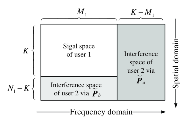
Figure 2: Space-Frequency dimension allocation for the two users when $K<N_{1}$.

After applying nulling matrix $\tilde{\boldsymbol{Q}}$, we have

$$\tilde{\boldsymbol{Q}}\tilde{\boldsymbol{y}}_{1}=\underbrace{\tilde{\boldsymbol{Q}}\tilde{\boldsymbol{H}}_{11}}_{\tilde{\boldsymbol{A}}}\tilde{\boldsymbol{x}}_{1}+\bigg{[}\underbrace{\tilde{\boldsymbol{Q}}\tilde{\boldsymbol{H}}_{12}\tilde{\boldsymbol{P}}_{a}}_{\tilde{\boldsymbol{B}}},\underbrace{\tilde{\boldsymbol{Q}}\tilde{\boldsymbol{H}}_{12}\tilde{\boldsymbol{P}}_{b}}_{\tilde{\boldsymbol{C}}}\bigg{]}\tilde{\boldsymbol{x}}_{2}+\tilde{\boldsymbol{Q}}\tilde{\boldsymbol{z}}_{1}.$$ (121)

To achieve the degrees of freedom pair shown in (115) for both users, it is sufficient to design our $\tilde{\boldsymbol{P}}$ and $\tilde{\boldsymbol{Q}}$ to satisfy the following conditions simultaneously

1. $\text{rank}(\tilde{\boldsymbol{A}})=M_{1}K$,

2. $\text{rank}([\tilde{\boldsymbol{P}}_{a},\tilde{\boldsymbol{P}}_{b}])=M_{2}(K-M_{1})+M_{1}(N_{1}-K)$,

3. $\tilde{\boldsymbol{B}}=\boldsymbol{0}$,

4. $\tilde{\boldsymbol{C}}=\boldsymbol{0}$.

We propose to use the following realizations:

$$\boldsymbol{Q}^{\textsf{F}} =[\boldsymbol{\mathcal{V}}_{K}(1,\omega_{K},\dots,\omega^{M_{1}-1}_{K})]^{T},$$ (122)

$$\boldsymbol{P}_{a}^{\textsf{F}} =\boldsymbol{\mathcal{V}}_{K}(\omega_{K}^{-M_{1}},\omega_{K}^{-(M_{1}+1)},\dots,\omega^{-(K-1)}_{K}).$$ (123)

$$\boldsymbol{P}_{b}^{\textsf{F}} =(\boldsymbol{Q}^{\textsf{F}})^{\dagger},$$ (124)

$$\boldsymbol{P}_{a}^{\textsf{S}} =\boldsymbol{I}_{M_{2}},$$ (125)

$$\boldsymbol{P}_{b}^{\textsf{S}} =[\boldsymbol{I}_{N_{1}-K};\boldsymbol{0}],$$ (126)

$$\boldsymbol{Q}^{\textsf{S}} =\text{null}(\boldsymbol{H}_{12}\boldsymbol{P}_{b}^{\textsf{S}})^{T},$$ (127)

where (127) means that $\boldsymbol{Q}^{\textsf{S}}\boldsymbol{H}_{12}\boldsymbol{P}_{b}^{\textsf{S}}=\boldsymbol{0}$. Here, we choose $((\boldsymbol{Q}^{\textsf{F}})^{\dagger},\boldsymbol{P}_{a}^{\textsf{F}})$ to be a size $K\times K$ IFFT matrix, which offers the same frequency domain explanation as discussed in Section IV-E; see also Fig. 2. It is trivial to see $\tilde{\boldsymbol{B}}=\boldsymbol{0}$. In other words, receiver 1 will simply ignore the signal in the last $K-M_{1}$ frequencies and only using the signal in the first $K$ frequencies to decode his own message. Therefore, $\tilde{\boldsymbol{P}}_{a}$ contains the interference directions from all the antennas of transmitter 2 but only in certain frequencies. Now, after applying the frequency nulling, there are $N_{1}K$ dimensions remaining, which contain both user 1’s message and the message of user 2 that is transmitted by $\tilde{\boldsymbol{P}}_{b}$. Among all the $N_{1}K$ dimensions, receiver 1 only requires $M_{1}K$ dimensions to decode his own message, while leaving additional $K(N_{1}-M_{1})$ dimensions for user 2. Here we choose one possible way of decomposing the remaining dimensions. Transmitter 2 sends some messages in the first $M_{1}$ frequencies but only though $N_{1}-K$ antennas, as shown in (126). Notice that

$$\tilde{\boldsymbol{C}} =\tilde{\boldsymbol{Q}}\tilde{\boldsymbol{H}}_{12}\tilde{\boldsymbol{P}}_{b}$$

$$=(\boldsymbol{Q}^{\textsf{F}}\otimes\boldsymbol{Q}^{\textsf{S}})(\boldsymbol{I}_{K}\otimes\boldsymbol{H}_{12})(\boldsymbol{P}_{b}^{\textsf{F}}\otimes\boldsymbol{P}^{\textsf{S}}_{b})$$ (128)

$$=(\boldsymbol{Q}^{\textsf{F}}\boldsymbol{P}_{b}^{\textsf{F}})\otimes(\boldsymbol{Q}^{\textsf{S}}\boldsymbol{H}_{12}\boldsymbol{P}^{\textsf{S}}_{b})$$ (129)

which means that the choice of $\boldsymbol{Q}^{\textsf{S}}$ as given in (127) is sufficient to set $\tilde{\boldsymbol{C}}=0$. It is clear that for the interference signal sent via $\tilde{\boldsymbol{P}}_{b}$, receiver 1 only need to do spatial zero-forcing in our scheme, which can be seen from the fact $\boldsymbol{Q}^{\textsf{F}}\boldsymbol{P}_{b}^{\textsf{F}}=\boldsymbol{I}_{K}$ due to (124).

To satisfy the second condition, notice that $\text{rank}(\tilde{\boldsymbol{P}}_{a})=M_{2}(K-M_{1})$ and $\text{rank}(\tilde{\boldsymbol{P}}_{a})=M_{1}(N_{1}-K)$, it is sufficient to show that $\tilde{\boldsymbol{P}}_{a}\perp\tilde{\boldsymbol{P}}_{b}$, which is obvious as

$$\tilde{\boldsymbol{P}}_{b}^{\dagger}\tilde{\boldsymbol{P}}_{a}=(\boldsymbol{Q}^{\textsf{F}}\boldsymbol{P}_{a}^{\textsf{F}})\otimes((\boldsymbol{P}^{\textsf{S}}_{b})^{\dagger}\boldsymbol{I}_{M_{2}})=\boldsymbol{0}$$ (130)

because $\boldsymbol{Q}^{\textsf{F}}\boldsymbol{P}_{a}^{\textsf{F}}=\boldsymbol{0}$. This is not surprising as the signal of user 2 transmitted via $\tilde{\boldsymbol{P}}_{a}$ and $\tilde{\boldsymbol{P}}_{b}$ are orthogonal in frequency domain. The remaining part is to show the first condition holds, which is true because here $\tilde{\boldsymbol{A}}$ has the same structure as $\tilde{\boldsymbol{A}}^{\prime}$ of (IV-D) with $N_{1}$ replaced by $K$ and $\boldsymbol{h}_{i}$ replaced by $\boldsymbol{Q}^{\textsf{S}}_{K\times N_{1}}\boldsymbol{h}_{i}$.

V-C Discussion

Figure 3: The benefit of antenna mode switching on the DoF region, in the case of $M_{1}<N_{1}<\min(M_{2},N_{2})$.

It is not surprising that when $K=N_{1}$, (53) implies

$$d_{1}+\frac{N_{1}}{\min(M_{2},N_{2})}d_{2}\leq N_{1}$$ (131)

which is the same as (7) and that in [17, Theorem 3] when $M_{1}<N_{1}<\min(M_{2},N_{2})$. For the scheme that we discussed above, $\tilde{\boldsymbol{P}}_{b}$ disappears and it is the DoF achievable scheme that we developed in Section IV-C. In addition, when $K=M_{1}$, (53) becomes (12) and $\tilde{\boldsymbol{P}}_{a}$ disappears, the general scheme reduces to the DoF-optimal spatial zero-forcing as shown in [24]. Hence, for one extra mode at transmitter 1, we can further align $\min(M_{2},N_{2})-N_{1}$ streams of interference over $K$ slots. The incremental gain per slot is reduced when $K$ increases; see Fig. 3. Our result reveals the fundamental benefit that can be obtained from reconfigurable antenna modes when there is no CSIT and $M_{1}<N_{1}<\min(M_{2},N_{2})$. In addition, combining with the known results, we know that in order to achieve the DoF region of two-user FIC and ZIC, zero-forcing in frequency and spatial domains suffice regardless of the CSIT assumption.

VI Conclusions

We derived the exact DoF region for the MIMO Z and full interference channels when perfect channel state information is available at receivers, including i) the Z interference channel with channel state information at the transmitter; ii) the Z and full interference channel without channel state information at the transmitter, but with reconfigurable antennas at the transmitters. For both FIC and ZIC, when the number of antenna modes $K$ at the transmitter with the reconfigurable antennas is not less than the number of receive antennas at the corresponding receiver, the DoF region is maximized and no longer depends on the number of antenna modes. Otherwise, each additional antenna mode can bring extra gain in the DoF region when $M_{1}<N_{1}<\min(M_{2},N_{2})$ for both FIC and ZIC, and when $M_{2}<N_{2}<\min(M_{1},N_{1})$ for FIC. The incremental gain diminishes as $K$ increases.

The achievability schemes we designed for the reconfigurable antenna cases rely on time expansion and joint beamforming and nulling over the time-expanded channel. Interestingly, they also bear a space-frequency coding interpretation. We completely characterized the DoF regions for both Z and full interference channels when transmitter antenna mode switching is allowed. Our result can specialize to previously known cases when there is no antenna mode switching by simply setting the number of antenna modes equal to the number of transmit antennas. Our work reveals how the channel variation introduced by the extra antenna mode switching brings benefits in the sense of the DoF region.

References

- [1] A. Carleial, “A case where interference does not reduce capacity (Corresp.),” IEEE Trans. Inform. Theory, vol. 21, no. 5, pp. 569–570, May 1975.
- [2] H. Sato, “The capacity of the Gaussian interference channel under strong interference (Corresp.),” IEEE Trans. Inform. Theory, vol. 27, no. 6, pp. 786–788, June 1981.
- [3] A. El Gamal and M. Costa, “The capacity region of a class of deterministic interference channels (Corresp.),” IEEE Trans. Inform. Theory, vol. 28, no. 2, pp. 343–346, Feb. 1982.
- [4] R. H. Etkin, D. N. C. Tse, and H. Wang, “Gaussian interference channel capacity to within one bit,” IEEE Trans. Inform. Theory, vol. 54, no. 12, pp. 5534–5562, Dec. 2008.
- [5] X. Shang, G. Kramer, and B. Chen, “Outer bound and noisy-interference sum-rate capacity for symmetric Gaussian interference channels,” in Information Sciences and Systems, 2008. CISS 2008. 42nd Annual Conference on, 2008, pp. 385–389.
- [6] V. Sreekanth Annapureddy and V. Veeravalli, “Sum capacity of the Gaussian interference channel in the low interference regime,” in Information Theory and Applications Workshop, 2008, 2008, pp. 422–427.
- [7] A. Motahari and A. Khandani, “Capacity bounds for the Gaussian interference channel,” in Proc. IEEE Intl. Symp. on Info. Theory, 2008, pp. 250–254.
- [8] G. Bresler and D. Tse, “The two-user Gaussian interference channel: a deterministic view,” European Trans. on Telecomm., vol. 19, no. 4, pp. 333–354, Apr. 2008.
- [9] G. Bresler, A. Parekh, and D. Tse, “The approximate capacity of the many-to-one and one-to-many gaussian interference channels,” 2008. [Online]. Available: http://arxiv.org/abs/0809.3554v1
- [10] S. Avestimehr, S. Diggavi, and D. Tse, “Wireless network information flow: a deterministic approach,” 2009. [Online]. Available: http://arxiv.org/abs/0906.5394
- [11] V. S. Annapureddy and V. V. Veeravalli, “Sum capacity of MIMO interference channels in the low interference regime,” 2009. [Online]. Available: http://arxiv.org/abs/0909.2074
- [12] X. Shang, B. Chen, G. Kramer, and H. V. Poor, “Capacity regions and sum-rate capacities of vector gaussian interference channels,” 2009. [Online]. Available: http://arxiv.org/abs/0907.0472
- [13] A. Goldsmith, S. Jafar, N. Jindal, and S. Vishwanath, “Capacity limits of MIMO channels,” IEEE Journal on Selected Areas in Communications, vol. 21, no. 5, pp. 684–702, May 2003.
- [14] V. Cadambe and S. Jafar, “Interference alignment and degrees of freedom of the K user interference channel,” IEEE Trans. Inform. Theory, vol. 54, no. 8, pp. 3425–3441, Aug. 2008.
- [15] S. Jafar and M. Fakhereddin, “Degrees of freedom for the MIMO interference channel,” IEEE Trans. Inform. Theory, vol. 53, no. 7, pp. 2637–2642, July 2007.
- [16] S. Jafar and S. Shamai, “Degrees of freedom region of the MIMO X channel,” IEEE Trans. Inform. Theory, vol. 54, no. 1, pp. 151–170, Jan. 2008.
- [17] C. Huang, S. Jafar, S. Shamai, and S. Vishwanath, “On degrees of freedom region of MIMO networks without CSIT,” 2009. [Online]. Available: http://arxiv.org/abs/0909.4017
- [18] Y. Zhu and D. Guo, “Isotropic MIMO interference channels without CSIT: The loss of degrees of freedom,” in Communication, Control, and Computing, 2009. Allerton 2009. 47th Annual Allerton Conference on, 2009, pp. 1338–1344.
- [19] C. S. Vaze and M. K. Varanasi, “The degrees of freedom regions of MIMO broadcast, interference, and cognitive radio channels with no CSIT ,” 2009. [Online]. Available: http://arxiv.org/abs/0909.5424
- [20] X. Shang, B. Chen, G. Kramer, and H. V. Poor, “MIMO Z-interference channels: capacity under strong and noisy interference,” 2009. [Online]. Available: http://arxiv.org/abs/0911.4530
- [21] Y. Zhu and D. Guo, “Ergodic fading one-sided interference channels without state information at transmitters,” 2009. [Online]. Available: http://arxiv.org/abs/0911.1082
- [22] S. A. Jafar, “Exploiting channel correlations - simple interference alignment schemes with no CSIT,” 2009. [Online]. Available: http://arxiv.org/abs/0910.0555
- [23] C. Wang, T. Gou, and S. A. Jafar, “Aiming perfectly in the dark - blind interference alignment through staggered antenna switching,” 2010. [Online]. Available: http://arxiv.org/abs/1002.2720
- [24] Y. Zhu and D. Guo, “The Degrees of Freedom of MIMO Interference Channels without State Information at Transmitters,” 2010. [Online]. Available: http://arxiv.org/abs/1008.5196
- [25] T. Jiang, N. Sidiropoulos, and J. ten Berge, “Almost-sure identifiability of multidimensional harmonic retrieval,” Signal Processing, IEEE Transactions on, vol. 49, no. 9, pp. 1849–1859, Sept. 2001.