THERMOHALINE MIXING: DOES IT REALLY GOVERN THE ATMOSPHERIC CHEMICAL COMPOSITION OF LOW-MASS RED GIANTS?

Abstract

First results of our 3D numerical simulations of thermohaline convection driven by ³He burning in a low-mass RGB star at the bump luminosity are presented. They confirm our previous conclusion that this convection has a mixing rate which is a factor of 50 lower than the observationally constrained rate of RGB extra-mixing. It is also shown that the large-scale instabilities of salt-fingering mean field (those of the Boussinesq and advection-diffusion equations averaged over length and time scales of many salt fingers), which have been observed to increase the rate of oceanic thermohaline mixing up to one order of magnitude, do not enhance the RGB thermohaline mixing. We speculate on possible alternative solutions of the problem of RGB extra-mixing, among which the most promising one that is related to thermohaline mixing is going to take advantage of the shifting of salt-finger spectrum towards larger diameters by toroidal magnetic field.

1 Introduction

Red giants with $M\lesssim 1.5\,M_{\odot}$ are known to experience extra-mixing in their convectively stable radiative zones that separate the hydrogen burning shell (HBS) from the bottom of the convective envelope (BCE). It operates during their first ascent along the red giant branch (RGB) above the bump luminosity, after the HBS has crossed a chemical composition discontinuity left behind by the BCE at the end of the first dredge-up. This causes the atmospheric ¹²C/¹³C ratio and carbon abundance to resume their declines with an increase in luminosity.

The most promising physical mechanism of RGB extra-mixing is thermohaline convection (Charbonnel & Zahn 2007a). It is driven by a double-diffusive instability that occurs when a scalar component that stabilizes a density stratification, e.g. the temperature $T$, diffuses away faster than a destabilizing component, e.g. the mean molecular weight $\mu$. Eggleton, Dearborn, & Lattanzio (2006) brought our attention to the fact that the reaction ³He(³He, 2p)⁴He produces a local depression of $\mu$, $\Delta\mu\sim-10^{-4}$, in the HBS tail above the bump luminosity. As a result, $\mu$ is increasing with the radius, which turns the $\mu$ profile into the destabilizing component. Moreover, the radiative thermal diffusivity $K$ exceeds the molecular diffusivity $\nu_{\rm mol}$ by many orders of magnitude (the inverse Lewis number $\tau=\nu_{\rm mol}/K\sim 10^{-6}$ in the region of $\mu$ depression), which should lead to the double-diffusive instability. In the ocean, a similar instability develops where warm salty water overlies cold fresh water. The oceanic thermohaline mixing usually takes the form of vertically elongated fluid parcels of rising fresh and sinking salty water adjacent to each other, called “salt fingers” (Stern 1960). It has extensively been studied both experimentally and theoretically (e.g., Kunze 2003).

The efficiency of thermohaline mixing in stellar cases can be estimated only theoretically, e.g. via a linear stability analysis of its governing equations (Ulrich 1972) or via direct numerical simulations. Denissenkov (2010, hereafter Paper I) has recently conducted a comparative study of thermohaline convection in the oceanic and RGB cases using both a linear stability analysis and 2D numerical simulations. Unfortunately, the linear theory yields a thermohaline diffusion coefficient that is proportional to the square of the (unknown) aspect ratio, $a=l/d$, of a finger, where $l$ and $d$ are the finger’s length and diameter. Applications of this diffusion coefficient to model the evolutionary decline of carbon abundance in low-mass red giants demand that $a>7$ (Paper I), which is in agreement with the original result of Charbonnel & Zahn (2007a). However, our 2D numerical simulations of ³He-driven thermohaline convection in the vicinity of a $\mu$ depression yield a mixing rate equivalent to that approximated by the linear-theory diffusion coefficient with $a<1$, i.e. it is a factor of $\sim 1/50^{\rm th}$ of its observationally constrained value. The difference in the finger aspect ratios between the oceanic ($a>1$) and RGB ($a<1$) cases is most likely determined by the very low viscosity $\nu$, or the Prandtl number $Pr=\nu/K\sim 10^{-6}$, in the RGB case. This facilitates the development of secondary shear instabilities that strongly limit the growth of salt fingers (Radko 2010, and Paper I). On the other hand, the diffusion coefficient for thermohaline convection with $a>7$ has been shown to reproduce many of the RGB extra-mixing observational patterns at all metallicities so well that we had to postpone further discussion of these findings until we were able to confirm or refute the results of our 2D numerical simulations using 3D computations.

In this Letter, we present first results of our 3D numerical simulations of thermohaline convection for the oceanic and RGB cases. It turns out that they do not differ much from the 2D results reported in Paper I. We also consider a possibility, mentioned in Paper I, that RGB thermohaline mixing may be enhanced by large-scale mean-field instabilities, such as the collective, $\gamma$-, and intrusive ones, that are known to occur in the ocean. Finally, we speculate on possible alternative solutions of the problem of RGB extra-mixing.

2 3D Numerical Simulations of Thermohaline Convection

The basic equations and numerical techniques that are employed in our 3D simulations of thermohaline convection for the oceanic and RGB cases are described in detail by Gargett, Merryfield, & Holloway (2003). They are very similar to those used in Paper I. The main goal of Gargett et al. was to study differential scalar diffusion in 3D stratified turbulence. Therefore, they considered a density stratification stable against the double-diffusive instability and used a specified turbulent velocity field as an initial condition. To apply their method and computer code for our purposes, we have made the slower diffusing component, which represents salinity $S$ in the ocean and $\mu$ in the current investigation, destabilizing by changing the sign of the vertical velocity term in their equation (16). We have also reduced the amplitude of the initial velocity field, so that it serves as a mild perturbation to initiate the double-diffusive instability. Our available computational resources have allowed us to run the code within reasonable time intervals with a spatial resolution of $320^{3}$. Simple estimates of the relevant turbulent kinetic energy dissipation rate and the Kolmogorov and Batchelor length scales show that this resolution is close to marginal for our runs, however, not fully resolving the slower-diffusing component has been shown not to have a large effect on the computed fluxes (Traxler et al. 2010). The 3D simulations have been carried out for the same number of fastest growing fingers in the computational domain and parameter sets from Table 1 in Paper I that were used in our 2D computations.

The blue and red solid curves in the upper left panel of Fig. 1 show transitions of the ratio $D_{S}/k_{T}$ to its equilibrium values in our 2D and 3D simulations of the oceanic thermohaline convection. Here, $D_{S}$ and $k_{T}$ are the turbulent salt and microscopic thermal diffusivities. The 2D simulations were performed with the resolution $1024^{2}$ (Paper I). Our estimated 3D equilibrium value of $D_{S}/k_{T}$ exceeds its corresponding 2D value merely by a factor of 1.5 (compare the blue and red dashed lines). It is in good agreement with the result obtained using a better resolution by Traxler et al. (2010) that we have interpolated for the value of density ratio $R_{\rho}=\alpha\Delta T/\beta\Delta S=1.6$ ($\alpha$ and $\beta$ are the coefficients of thermal expansion and haline contraction) from their Table 1 (star symbol). The upper right panel makes a similar comparison for the RGB thermohaline convection. In this case, we do not find any difference between the 2D and 3D equilibrium values of the ratio $D_{\mu}/K$ (the blue and red dashed lines coincide). Therefore, we conclude that our results reported in Paper I seem to be correct. In particular, RGB thermohaline convection driven by ³He burning yields a turbulent mixing rate that is by a factor of 50 lower than the value required by observations.

3 Mean-Field Instabilities

Observations, laboratory experiments, and direct numerical simulations show that small-scale salt-fingering convection in the ocean can lead to instabilities and the formation of dynamical structures on much larger scales. These include the so-called “collective instability” leading to the generation of internal gravity waves, the intrusive instability developing when fluid is stratified both vertically and horizontally (in stars, such a situation may result from the rotational distortion of level surfaces), and the so-called “$\gamma$-instability” that produces thermohaline staircases (e.g., see Traxler et al. 2010, and references therein). The latter structures consist of thick well-mixed convective layers separated by thin salt-fingering interfaces. The staircases are of special interest to us because they have been observed to enhance vertical mixing in the ocean by up to an order of magnitude (Schmitt et al. 2005). Moreover, our preliminary estimates in Paper I indicate that the turbulent flux ratio $\gamma=F_{T}/F_{\mu}$ is a decreasing function of $R_{\rho}$ in the RGB case, which is a sufficient condition for the $\gamma$-instability, according to Radko (2003).

The large-scale instabilities are studied by averaging the Boussinesq and advection-diffusion equations for $T$ and $S$ ($\mu$) over length and time scales of many salt fingers. As a result, a system of mean-field equations is obtained in which the small-scale turbulent velocity is incorporated into the mean heat and salinity fluxes $F_{T}$ and $F_{S}$ (Traxler et al. 2010). The fluxes are related to one another and to the large-scale temperature gradient via the flux ratio $\gamma=F_{T}/F_{S}$ and the Nusselt number $Nu$, which are assumed to depend only on the local value of the density ratio $R_{\rho}$; specification of these dependences closes the mean-field equations. Large-scale changes in $R_{\rho}$ thus result in modulations of $F_{T}$ and $F_{S}$ via the dependences of $\gamma$ and $Nu$ on $R_{\rho}$ that can either amplify or damp initial perturbations.

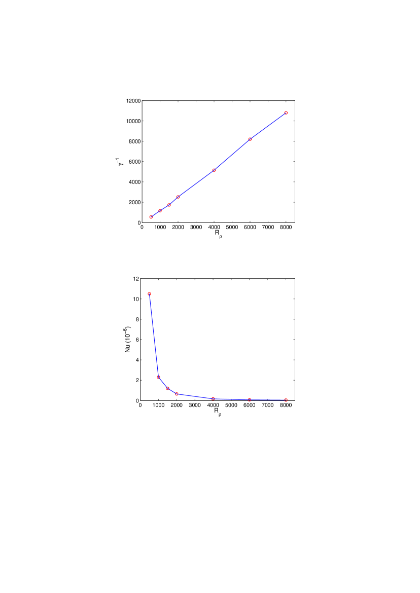
Figure 2: The inverse flux ratio, $\gamma^{-1}=F_{\mu}/F_{T}$, and Nusselt number as functions of density ratio estimated from our 2D numerical simulations of the RGB thermohaline convection.

A linear stability analysis of the mean-field equations yields a third-order dispersion relationship for the growth rates of all the three large-scale instabilities mentioned above (equation 2.13 of Traxler et al. 2010). Coefficients of the cubic equation depend on the Prandtl and inverse Lewis numbers as well as on $Nu$, $\gamma$ and their derivatives with respect to $R_{\rho}$. The coefficients are also functions of the horizontal and vertical wavenumbers, $l$ and $k$. To calculate them, we first need to estimate the dependences of $Nu$ and $\gamma$ on $R_{\rho}$. Traxler et al. (2010) estimated those dependences via a body of 3D numerical simulations of the oceanic salt-fingering convection. We have used data from their Table 2 to reproduce, for a comparison, their “flower plot” depicting the growth rates of fastest growing instabilities at $R_{\rho}=1.5$ in the absence of lateral gradients (the lower left panel of Fig. 1). The bulb of the flower corresponds to the salt-fingering mode that turns out to be a solution of the general dispersion equation as well. The leaves of the flower represent the gravity waves of the collective instability, whereas the $\gamma$-instability modes are the ones dominating in the region beneath the leaves. To obtain estimates of $\gamma(R_{\rho})$ and $Nu(R_{\rho})$ for the RGB case (Fig. 2), we have performed additional 2D numerical simulations of the ³He-driven thermohaline convection for the same parameter set that was used in Paper I but for a number of different values of $R_{\rho}$. The resulting flower plot is shown in the lower right panel of Fig. 1. We see that in the RGB case only the salt-fingering mode is unstable in spite of the flux ratio $\gamma$ being a decreasing function of $R_{\rho}$, as in the oceanic case. This difference is explained by the fact that the Nusselt number is extremely small, $Nu\sim 10^{-6}$, in the RGB case. Because of this, it is necessary to include horizontal diffusive fluxes in the mean-field stability analysis — something which was not done by Radko (2003) but was treated by Traxler et al. (2010). In the RGB case, the inclusion of reasonable lateral gradients proportional to their corresponding vertical gradients multiplied by the ratio of centrifugal to gravitational acceleration only produces an asymmetry of the bulb with respect to the vertical axis.

4 Possible Alternative Solutions

Our 2D and 3D numerical simulations of thermohaline convection driven by ³He burning have demonstrated that it is unlikely to be the sole mechanism of RGB extra-mixing. Its corresponding mixing rate in the vicinity of a $\mu$ depression, $D_{\mu}\approx 2\times 10^{-3}\,K$ (the upper right panel of Fig. 1), is too low compared to the observationally constrained value of $(D_{\mu})_{\rm obs}\approx 0.1\,K$ (Paper I). Therefore, for its efficiency to be consistent with observations, the RGB thermohaline mixing has to be either assisted or modified by other processes. In Paper I, we have shown that a turbulent viscosity $\nu_{\rm t}$ exceeding the microscopic one by a factor of $10^{4}$ could enhance the rate of ³He-driven thermohaline mixing up to the observed value, provided that it was not itself associated with strong turbulent mixing. The enhancement of thermohaline mixing in this case is caused by the fact that the higher viscosity suppresses the development of secondary shear instabilities that limit the growth of salt fingers. On the other hand, if the increase of viscosity is accompanied by a similar increase of the rate of turbulent mixing, the latter will reduce salt-finger buoyancy and vertical transports by smoothing out the chemical composition contrast between rising and sinking fluid parcels.

The additional source of turbulence in the radiative zones of RGB stars could arise from the differential rotation that is produced by the mass inflow that feeds the HBS (Paper I). We have employed the COMSOL Multiphysics software package to solve the angular momentum transport equation for the radiative zone of the low-metallicity bump-luminosity RGB model from Paper I in the presence of mass inflow and turbulent shear mixing. Their respective rate $\dot{r}$ and diffusion coefficient $\nu_{\rm v}$ are given by equation (23) from Paper I and equation (3) with the uncertainty factor $f_{\rm v}$ from the paper of Denissenkov, Chaboyer, & Li (2006). The angular velocity at the BCE was assumed to have the same value, $\Omega_{\rm BCE}=6.3\times 10^{-7}$ rad s^-1, as in the M2 bump-luminosity RGB model of Palacios et al. (2006). Simple estimates show that for $f_{\rm v}\gtrsim 1$ the transport of angular momentum by the rotation-induced turbulent diffusion dominates over its advection by meridional circulation, therefore, and for the sake of simplicity, the latter was neglected. Our computations show that the competition between the terms proportional to $\dot{r}$ and $\nu_{\rm v}$ leads to a stationary solution with $\nu_{\rm v}\approx 3\times 10^{-4}\,K$ in the vicinity of a $\mu$ depression that very weakly depends on both $f_{\rm v}$ and $\Omega_{\rm BCE}$, although the final rotational shear is a decreasing function of $f_{\rm v}$. This value exceeds the microscopic viscosity by a factor of $10^{2}$, which is not enough to enhance $D_{\mu}$ to its observed value (Paper I). It is also difficult to understand why the rotation-induced small-scale turbulence should not produce a mixing rate of the same magnitude as $\nu_{\rm v}$, in which case $D_{\mu}$ will not be enhanced at all (Paper I). Therefore, we do not think that the proposed viscosity enhancement is a possible solution of the problem.

Our angular momentum transport computations confirm the conclusion that radiative zones of low-mass RGB stars above the bump luminosity should possess strong differential rotation. This may lead to the generation of high-amplitude toroidal magnetic fields, especially close to the HBS, provided that a weak poloidal field is present in the radiative zone. Under these circumstances, a possible alternative solution of the problem could be magneto-thermohaline mixing (Denissenkov, Pinsonneault, & MacGregor 2009). We intend to investigate this possibility using 2D numerical simulations in one of our forthcoming papers.

Toroidal magnetic fields in radiative zones may also filter out salt fingers with small diameters, so that the maximum growth rate is shifted towards thicker fingers. Since the finger growth rate decreases with an increase in diameter as $\sigma\propto d^{-2}$ (e.g., Paper I), the square of the vertical velocity shear between the axes of neighbouring rising and sinking fingers, $\sim(\sigma l/d)^{2}$, is proportional to $a^{2}d^{-4}$. This parameter is likely to control the development of secondary shear instabilities (Kunze 1987); consequently, thicker fingers will probably reach higher aspect ratios before they are destroyed. Following Charbonnel & Zahn (2007b), we have complemented the dispersion relationship (13) from Paper I (note that the term $\nu k_{T}k_{S}k^{6}$ was erroneously omitted) with terms that take into account the Lorentz force associated with a specified toroidal magnetic field $B_{0}$. Its solutions are shown in Fig. 3 for the field strengths $B_{0}=0$, 10, and 100 G (the solid blue curves from left to right). In the case of $B_{0}=100$ G, the fastest growing fingers transverse to the field have a diameter that is nearly 40 times as large as that of fingers in the absence of a magnetic field. This diameter is also almost four times larger than the diameter of fastest growing fingers in the case of a viscosity that is amplified by the factor of $10^{4}$ (the red solid curve). However the influence of such a field on the planform of the fastest growing fingers still needs to be studied. In our next study, we will perform 2D numerical simulations of the RGB thermohaline convection in the presence of a toroidal magnetic field to find out if the magnetic shift of the salt-finger growth-rate spectrum towards larger diameters can really enhance its associated mixing rate up to the empirically constrained value.

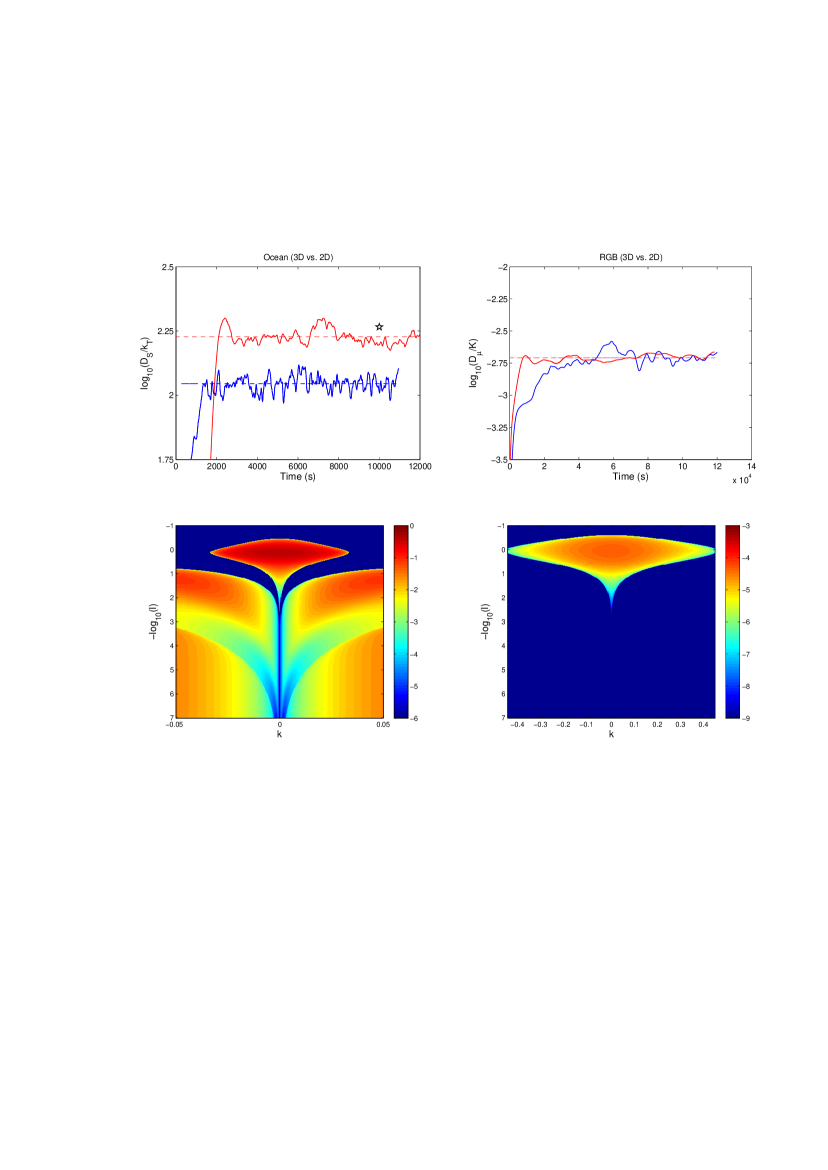
Figure 1: Upper panels compare the ratios of thermohaline diffusion coefficient to thermal diffusivity obtained in our 3D (red curves) and 2D (blue curves) numerical simulations for the oceanic (left) and RGB (right) cases. Black star symbol shows a value interpolated for the density ratio $R_{\rho}=1.6$ using the higher resolution 3D data of Traxler et al. (2010). Lower panels depict the decimal logarithms of growth rates (s^-1) of the fastest growing large-scale instabilities of salt-fingering mean-field as functions of the horizontal $l$ and vertical $k$ wavenumbers, both measured in cm^-1, for the oceanic (left) and RGB (right) cases.

Figure 3: The RGB salt-finger growth-rate spectra computed for the same parameter set as in Table 1 from Paper I under the assumptions that the toroidal magnetic field has the strengths $B_{0}=0$, 10, and 100 G (the blue curves from left to right), and for $B_{0}=0$ G but with the viscosity amplified by the factor of $10^{4}$ (the red curve).

References

- Charbonnel & Zahn (2007a) Charbonnel, C., & Zahn, J.-P. 2007a, A&A, 467, L15
- Charbonnel & Zahn (2007b) Charbonnel, C., & Zahn, J.-P. 2007b, A&A, 476, L29
- Denissenkov (2010) Denissenkov, P. A. 2010, ApJ, 723, 563 (Paper I)
- Denissenkov, Pinsonneault, & MacGregor (2009) Denissenkov, P. A., Pinsonneault, M. H., & MacGregor, K. B. 2009, ApJ, 696, 1823
- Denissenkov, Chaboyer, & Li (2006) Denissenkov, P. A., Chaboyer, B., & Li, K. 2006, ApJ, 641, 1087
- Eggleton, Dearborn, & Lattanzio (2006) Eggleton P. P., Dearborn, D. S. P., & Lattanzio, J. C. 2006, Science, 314, 1580
- Gargett, Merryfield, & Holloway (2003) Gargett A. E., Merryfield, W. J., & Holloway, G. 2003, JPO, 33, 1758
- Kunze (2003) Kunze, E. 2003, POce, 56, 399
- Kunze (1987) Kunze, E. 1987, Journal of Marine Research, 45, 533
- Palacios et al. (2006) Palacios, A., Charbonnel, C., Talon, S., & Siess, L. 2006, A&A, 453, 261
- Radko (2003) Radko, T. 2003, JFM, 497, 365
- Radko (2010) Radko, T. 2010, JFM, 645, 121
- Schmitt et al. (2005) Schmitt, R. W., Ledwell, J. R., Montgomery, E. T., Polzin, K. L., & Toole, J. M. 2005, Sci., 308, 685
- Stern (1960) Stern, M. E. 1960, Tellus, 12, 172
- Traxler et al. (2010) Traxler, A., Stellmach, S., Garaud, P., Radko, T., & Brummell, N. 2010, arXiv:1008.1807v1 [physics.flu-dyn]
- Ulrich (1972) Ulrich, R. K. 1972, ApJ, 172, 165