Probing the course of cosmic expansion with a combination of observational data

Abstract

We study the cosmic expansion history by reconstructing the deceleration parameter $q(z)$ from the SDSS-II type Ia supernova sample (SNIa) with two different light curve fits (MLCS2k2 and SALT-II), the baryon acoustic oscillation (BAO) distance ratio, the cosmic microwave background (CMB) shift parameter, and the lookback time-redshift (LT) from the age of old passive galaxies. Three parametrization forms for the equation of state of dark energy (CPL, JBP, and UIS) are considered. Our results show that, for the CPL and the UIS forms, MLCS2k2 SDSS-II SNIa+BAO+CMB and MLCS2k2 SDSS-II SNIa+BAO+CMB+LT favor a currently slowing-down cosmic acceleration, but this does not occur for all other cases, where an increasing cosmic acceleration is still favored. Thus, the reconstructed evolutionary behaviors of dark energy and the course of the cosmic acceleration are highly dependent both on the light curve fitting method for the SNIa and the parametrization form for the equation of state of dark energy.

I INTRODUCTION

One of the most important and mysterious issues of modern cosmology is the fact that our universe is undergoing an accelerating expansion expansion1 ; expansion2 . This observed phenomenon is usually attributed to the existence of an exotic energy component called dark energy (DE), which generates a repulsive force due to the negative pressure associated with it. The simplest candidate of DE is the cosmological constant with the equation of state (EOS) $w=-1$. If one generalizes the EOS $w$ of DE from $w=-1$ to be an arbitrary constant $w$, the current astronomical observations observation1 ; observation2 ; observation3 show that $w$ is confined to be $|1+w|<0.06$ at the $1\sigma$ confidence level. However, the EOS might also be a function of cosmic time. In order to unveil the evolutionary properties of dark energy using observations, one usually adopts a parametrization form with some free parameters for $w(z)$, which may not be motivated by any particular foundamental theory. Examples of such kind are the Chevallier-Polarski-Linder (CPL) parametrization CPL , the Jassal-Bagla-Padmanabhan (JBP) parametrization JBP as well as the Upadhye-Ishak-Steinhardt (UIS) parametrization UIS , and so on. Constraining the free parameters of a given parametrization with observational data, one can obtain the evolutionary curve of $w(z)$, which embodies the property of dark energy. For instance, some current observations give an indication that the EOS has crossed the phantom divider ($w=-1$) at least once cross1 ; cross2 .

Recently, Sahni et al. proposed a new diagnostic of DE, named $Om(z)$ diagnostic. The advantage of this diagnostic, as opposed to the EOS, is that it depends on the first derivative of the luminosity distance $d_{L}(z)$ diagnostic , and thus is less sensitive to the observational errors and the present matter energy density $\Omega_{0m}$. In addition, one can discriminate DE models with the EOS $w<-1,w=-1$ and $w>-1$ effectively by examining the slope of $Om(z)$ even if the value of $\Omega_{0m}$ is not exactly known, with positive, null, or negative slopes corresponding to $w<-1,w=-1$ or $w>-1$, respectively.

Performing the $Om(z)$ diagnostic diagnostic and analyzing the deceleration parameter $q(z)$ with the Constitution type Ia supernova data (SNIa) constitution and data from the baryon acoustic oscillation (BAO) distance ratio of the distance measurements obtained at $z=0.2$ and $z=0.35$ in the galaxy power spectrum bao1 ; bao2 by using the popular CPL parametrization, Shafieloo et al. found that $Om(z)$ and $q(z)$ increases markedly at the low redshifts $z<0.3$ slowing . This result suggests that the expansion acceleration of our universe is probably slowing down. However, the result obtained from a combination of the cosmic microwave background (CMB) shift parameter, SNIa and BAO is very well consistent with the $\Lambda$CDM model. So, there appears some tension between low redshift data (Constitution SNIa+BAO) and high redshift (CMB) one. Surprisingly, further analysis using a subsample (SNLS+ESSENCE+CfA) of the Constitution SNIa reveals that the outcome does not rely on whether the CMB data is added and the cosmic acceleration has been over the peak. It was therefore argued the tension could be either due to the systematics in some data or that the CPL parametrization is not versatile-enough to accommodate the evolution of DE implied by the data. This situation was also examined by Gong et al. gong recently through the reconstruction of $Om(z)$. They found that both the systematics in data sets and the parametrization of DE influence the evolutional behavior of DE. It is worth noting that the results in Ref. slowing are obtained only at the $1\sigma$ confidence level and whether they are reliable at the $2\sigma$ confidence level still needs to be checked.

In this paper, we will re-examine this issue with three different parametrization forms for the EOS of DE (CPL, JBP and UIS CPL ; JBP ; UIS ), and 288 SNIa data points released by the Sloan Digital Sky Survey-II (SDSS-II) Supernova Survey with two different light curve fits (MLCS2k2 fit and SALT-II fit). We hope this will help us further understand the influence of different light curve fitting methods . As in slowing , the BAO distance ratio and the CMB shift parameter are also considered in our analysis. In addition, we use the lookback time-redshift (LT) from the age of old passive galaxies, since it has the advantage that the ages of distant objects are independent of each other, and thus may avoid biases that are present in techniques using distances of primary or secondary indicators in the cosmic distance ladder method.

II PARAMETRIZATION

By assuming that the energy components of our universe are nonrelativistic matter and dark energy, the Friedmann equation can be expressed as

$$E^{2}(z)=\frac{H^{2}(z)}{H_{0}^{2}}=\Omega_{0m}(1+z)^{3}+\Omega_{DE},$$ (1)

where $\Omega_{0m}$ is the current value of the dimensionless matter energy density, and $\Omega_{DE}$ is the dimensionless energy density parameter of dark energy, which can be expressed as

$$\Omega_{DE}=(1-\Omega_{0m})\exp\bigg{[}3\int_{0}^{z}\frac{1+w(z^{\prime})}{1+z^{\prime}}dz^{\prime}\bigg{]}\;,$$ (2)

where $w(z)$ is the equation of state of dark energy.

Now, we consider three parametrization forms for the EOS. i.e., the CPL, JBP and UIS parametrization. The EOS $w(z)$ for the CPL is CPL

$$w(z)=w_{0}+\frac{w_{1}z}{1+z}.$$ (3)

Substituting it into Eqs. (1, 2), one has

$$E^{2}(z)=\Omega_{0m}(1+z)^{3}+(1-\Omega_{0m})(1+z)^{3(1+w_{0}+w_{1})}\exp\bigg{(}-\frac{3w_{1}z}{1+z}\bigg{)}\;.$$ (4)

For the JBP parametrization, $w(z)$ is JBP

$$w(z)=w_{0}+\frac{w_{1}z}{(1+z)^{2}}\;.$$ (5)

So we have

$$E^{2}(z)=\Omega_{0m}(1+z)^{3}+(1-\Omega_{0m})(1+z)^{3(1+w_{0})}\exp\bigg{(}\frac{3w_{1}z^{2}}{2(1+z)^{2}}\bigg{)}\;.$$ (6)

And for the UIS parametrization UIS , the $w(z)$ and $E^{2}(z)$ can be expressed respectively as,

$$w(z)=\begin{cases}w_{0}+w_{1}z~{}~{}&\mbox{$z<1$},\\ w_{0}+w_{1}~{}~{}&\mbox{$z\geq 1$,}\end{cases}$$ (7)

and

$$E^{2}(z)=\begin{cases}\Omega_{0m}(1+z)^{3}+(1-\Omega_{0m})(1+z)^{3(1+w_{0}-w_{1})}\exp(3w_{1}z)~{}~{}&\mbox{$z<1$},\\ \Omega_{0m}(1+z)^{3}+(1-\Omega_{0m})(1+z)^{3(1+w_{0}+w_{1})}~{}~{}&\mbox{$z\geq 1$.}\end{cases}$$ (8)

III OBSERVATIONAL DATA

The SNIa dataset used in our analysis is the 288 data points released by the Sloan Digital Sky Survey-II (SDSS-II) Supernova Survey Kessler , which consist of $103$ new SNIa from the first-year SDSS-II supernova survey Frieman ; Sako ; Kessler , 56 points from ESSENCE Wood-Vasey , 62 from SNLS Astier , 34 from HST Riess , and 33 nearby SNIa Jha . For 288 SDSS-II SNIa data, two kinds of light curve fitting methods, i.e., the MLCS2k2 fit and the SALT-II fit, have been employed Kessler . Here, for the sake of systematics influence check, we do our analysis of the SDSS-II data with both kinds of fits.

The constraints from the SNIa data can be obtained by minimizing the following $\chi^{2}$ statistics:

$$\chi_{\mu}^{2}(\mu_{0},\textbf{p})=\sum_{i=1}^{288}\frac{[\mu_{obs,i}-\mu_{th}(z_{i};\mu_{0},\textbf{p})]^{2}}{\sigma_{\mu}^{2}},$$ (9)

where $\mu_{obs,i}$ is the distance modulus estimated from the MLCS2K2 fit or SALT-II fit for the i’th supernova, $z_{i}$ is its spectroscopically determined redshift, p stands for the complete set of model parameters, and $\mu_{th}(z_{i};\textbf{p})$ is the theoretical distance modulus for a concrete cosmological model, which is calculated from

$$\mu_{th}(z_{i};\mu_{0},\textbf{p})=5\log_{10}(d_{L}(z_{i};\textbf{p}))+\mu_{0},$$ (10)

where $d_{L}$ represents the luminosity distance. For a flat universe, $d_{L}$ is given by

$$d_{L}(z;\textbf{p})=(1+z)\int_{0}^{z}dz^{\prime}\frac{1}{E(z^{\prime},\textbf{p})}.$$ (11)

Let us note that here $\mu_{0}$ is a nuisance parameter. In order to marginalize over it, we expand $\chi_{\mu}^{2}$ (Eq. (9)) with respect to $\mu_{0}$ as

$$\chi_{\mu}^{2}(\mu_{0},\textbf{p})=A-2\mu_{0}B+\mu_{0}^{2}C\;,$$ (12)

where

$$A(\textbf{p})=\sum_{i=1}^{288}\frac{[\mu_{obs,i}-\mu_{th}(z_{i};\mu_{0}=0,\textbf{p})]^{2}}{\sigma_{\mu}^{2}}\;,$$ (13)

$$B(\textbf{p}) = \sum_{i=1}^{288}\frac{[\mu_{obs,i}-\mu_{th}(z_{i};\mu_{0}=0,\textbf{p})]}{\sigma_{\mu}^{2}}\;,$$ (14)

$$C = \sum_{i=1}^{288}\frac{1}{\sigma_{\mu}^{2}}\;.$$ (15)

Eq. (12) has a minimum at $\mu_{0}=B/C$, and it is

$$\tilde{\chi}_{\mu}^{2}(\textbf{p})=A(\textbf{p})-\frac{B(\textbf{p})^{2}}{C}\;.$$ (16)

Thus, instead of minimizing $\chi_{\mu}^{2}(\mu_{0},\textbf{p})$, we can minimize $\tilde{\chi}_{\mu}^{2}(\textbf{p})$, which is independent of $\mu_{0}$, to obtain constraints on the model parameters.

In the $\chi_{\mu}^{2}$-expression, the distance-modulus uncertainty is given by

$$\sigma_{\mu}^{2}=(\sigma_{\mu}^{fit})^{2}+(\sigma_{\mu}^{int})^{2}+(\sigma_{\mu}^{z})^{2},$$ (17)

where $\sigma_{\mu}^{fit}$ and $\sigma_{\mu}^{int}$(=0.16 for MLCS2k2 and 0.14 for SALT-II) are respectively the statistical uncertainty and the additional (intrinsic) error derived from light-curve fitting method. $\sigma_{\mu}^{int}$ is introduced to unitize $\chi^{2}$ per degree of freedom for the Hubble diagram constructed from the nearby SNIa sample and it is detailed in Ref. Kessler . It has little effect on the results of model parameters, but improves the value of $\chi^{2}_{\mu}$ remarkably. For example, for SALT-II SNIa with and without $\sigma_{\mu}^{int}$, the best fit values of the CPL parametrization are $w_{0}=-1.022$ and $w_{1}=0.090$ with $\chi^{2}_{\mu}=268.66$, and $w_{0}=-1.015$ and $w_{1}=0.200$ with $\chi^{2}_{\mu}=589.31$, respectively, where $\Omega_{0m}$ is given prior to be $0.262$ obtained from WMAP7 WMAP7 . $\sigma_{\mu}^{z}$ is the error which relates with the redshift uncertainty and can be computed from

$$\sigma_{\mu}^{z}=\sigma_{z}\bigg{(}\frac{5}{\ln 10}\bigg{)}\frac{1+z}{z(1+z/2)},$$ (18)

where $\sigma_{z}^{2}$ is the redshift uncertainty and is defined to be

$$\sigma_{z}^{2}=\sigma_{z,spec}^{2}+\sigma_{z,pec}^{2}.$$ (19)

Here, $\sigma_{z,spec}$ and $\sigma_{z,pec}$, as discussed in detail in Ref. Kessler , are the uncertainties from spectroscopic measurements and peculiar motion of the host galaxy, respectively.

The BAO distance measurements used in our analysis are obtained at $z=0.2$ and $z=0.35$ from the joint analysis of the 2dF Galaxy Redshift Survey and SDSS data bao2 . The BAO distance ratio

$$\frac{D_{V}(z=0.35)}{D_{V}(z=0.20)}=1.736\pm 0.065$$ (20)

is a relatively model-independent quantity. Here $D_{V}(z)$ is defined as

$$D_{V}(z_{BAO})=\bigg{[}\frac{z_{BAO}}{H(z_{BAO})}\bigg{(}\int_{0}^{z_{BAO}}\frac{dz}{H(z)}\bigg{)}^{2}\bigg{]}^{1/3}.$$ (21)

For the BAO dataset, we can fit the model parameter $\mathbf{p}$ by performing $\chi^{2}$ statistics as follows

$$\chi_{BAO}^{2}(\mathbf{p})=\frac{[D_{V}(z=0.35)/D_{V}(z=0.20)-1.736]^{2}}{0.065^{2}}\;.$$ (22)

In addition to the low redshift SNIa and BAO, we add the high redshift CMB parameter which is the reduce distance at $z_{ls}=1090$. The shift parameter

$$R(\textbf{p})=\sqrt{\Omega_{0m}}\int_{0}^{z_{ls}}\frac{dz}{E(z,\textbf{p})}=1.71\pm 0.019,$$ (23)

is used. We also apply $\chi^{2}$

$$\chi^{2}_{CMB}(\mathbf{p})=\frac{[R(\mathbf{p})-1.71]^{2}}{0.019^{2}}$$ (24)

to the model parameter $\mathbf{p}$ for the CMB data.

Besides the most common observational data sets above, we also perform an analysis combined with the lookback time-redshift data (LT), which is established by estimating the age of 32 old passive galaxies distributed over the redshift interval $0.11\leq z\leq 1.84$ and the total age of the universe $t_{0}^{obs}$ Simon . The galaxy samples of passively evolving galaxies are selected with high-quality spectroscopy and the method used to determine ages of galaxy samples indicates that systematics are not a serious source of error for these high-redshift galaxies. In addition, this data set has the advantage that the ages of distant objects are independent of each other, and thus it may avoid biases that are present in techniques that use distances of primary or secondary indicators in the cosmic distance ladder method. As a result, these age data are different from the widely used distance one, such as SNIa, and it may help us gain more insight into the nature of dark energy. To estimate the best fit of model parameters, we minimize $\chi_{age}^{2}$

$$\chi_{age}^{2}(\mathbf{p})=\sum\limits_{i}\frac{\big{[}t_{L}(z_{i};\textbf{p})-t_{L}^{obs}(z_{i};\tau)\big{]}^{2}}{\sigma_{T}^{2}}+\frac{\big{[}t_{0}(\textbf{p})-t_{0}^{obs}\big{]}}{\sigma_{t_{o}^{obs}}^{2}},$$ (25)

where, $\sigma_{T}^{2}\equiv\sigma_{i}^{2}+\sigma_{t_{0}^{obs}}^{2}$, $\sigma_{i}$ is the uncertainty in the individual lookback time to the $i^{th}$ galaxy of the sample, $\sigma_{t_{0}^{obs}}=0.7~{}Gyr$ stands for the uncertainty in the total expansion age of the universe ($t_{0}^{obs}$), and $\tau$ means the time from Big Bang to the formation of the object, which is the so-called delay factor or incubation time. Note that while the observed lookback time ($t_{L}^{obs}(z_{i};\tau)$) is directly dependent on $\tau$, its theoretical value ($t_{L}(z_{i};\textbf{p})$) is not. Furthermore, in principle, it must be different for each object in the sample. Thus the delay factor becomes a “nuisance” parameter, we use the following method to marginalize over it obl ; modlike

$$\tilde{\chi}^{2}(\mathbf{p}) = -2\ln\int_{0}^{\infty}d\tau\exp\bigg{(}-\frac{1}{2}\chi_{age}^{2}\bigg{)}$$ (26)

$$= A-\frac{B^{2}}{C}+D-2\ln\bigg{[}\sqrt{\frac{\pi}{2C}}\textrm{erfc}\bigg{(}\frac{B}{\sqrt{2C}}\bigg{)}\bigg{]},$$

where

$$A=\sum_{i=1}^{n}\frac{\triangle^{2}}{\sigma_{T}^{2}}.~{}~{}~{}~{}~{}~{}~{}~{}~{}~{}~{}~{}~{}~{}B=\sum_{i=1}^{n}\frac{\triangle}{\sigma_{T}^{2}}.~{}~{}~{}~{}~{}~{}~{}~{}~{}~{}~{}~{}~{}~{}C=\sum_{i=1}^{n}\frac{1}{\sigma_{T}^{2}},$$ (27)

D is the second term of the rhs of Eq. (25),

$$\triangle=t_{L}(z_{i};\textbf{p})-[t_{0}^{obs}-t(z_{i})],$$ (28)

and $\textrm{erfc}(x)$ is the complementary error function of the variable $x$.

IV RESULTS

We first explore three popular parametrization forms by using SDSS-II SNIa, BAO and CMB. A comparison of two light curve fits of SDSS-II SNIa is given. The results are shown in Figs. (1, 2).

Fig. (1) gives the contour diagrams on $w_{0}-w_{1}$ panel at the $68.3\%$ and $95.4\%$ confidence levels for three parametrization forms. Since different data sets give different best fit values of $\Omega_{0m}$, we set prior $\Omega_{0m}=0.262$ in this paper, which is the best fit value from the WMAP7 WMAP7 . The top, middle, and bottom panels are the results of the CPL, JBP and UIS, respectively. The big red points denote the spatially flat $\Lambda$CDM model ($w_{0}=-1$ and $w_{1}=0$). In the left panels, the SNIa is obtained with the SALT-II light curve fit, whereas, in the right panels, it is given with the MLCS2k2 one. The blue dotted, yellow dot-dashed, green dashed and pink solid lines show the results from SDSS-II SNIa, BAO+CMB, SDSS-II SNIa+BAO, and SDSS-II SNIa+BAO+CMB, respectively. From this figure, it is interesting to see that, for all three different parametrization forms, the $\Lambda$CDM model is consistent with the SNIa, SNIa+BAO and SNIa+BAO+CMB at the $1\sigma$ confidence level when the SALT-II fit is used. This consistency is, however, broken at the $2\sigma$ confidence level when the fit is changed to MLCS2k2. Thus, the consistency of the $\Lambda$CDM model with data depends crucially on the type of fit used. This agrees with what was obtained in Ref. Sanchez2009 from the SDSS-II SNIa with the CPL parametrization. Let us note that this discrepancy between two analysis methods has been pointed out in Refs. Nesseris2005 ; Jassal2006 , and it was also found with a simple $w$CDM model in the original SDSS-II paper Kessler . Furthermore, we find that the SDSS-II SNIa with SALT-II fit is consistent with BAO+CMB very well. However, when the MLCS2k2 fit is used, there exists a tension between SNIa and CMB+BAO at the $1\sigma$ confidence level. Actually, this tension also exists between other SNIa sets, Gold, for an example, and CMB+BAO Jassal2005 .

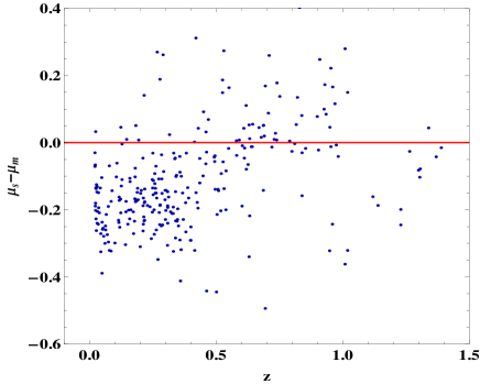
Figure 3: The difference in the distance modulus obtained with two fits for each supernova. The subscripts $s$ and $m$ represent the SALT-II fit and the MLCS2k2 fit respectively.

Fig. (2) shows the evolutionary curves of the deceleration parameter $q(z)$ reconstructed from the SDSS-II SNIa (SALT-II and MLCS2k2)+BAO and the SDSS-II SNIa+BAO+CMB for three parametrization forms. The gray regions and the regions between the two dashed lines represent the $1\sigma$ confidence level for $q(z)$ obtained from SNIa+BAO+CMB and SNIa+BAO, respectively. The dot-dashed lines show the best fit curves of the spatially flat $\Lambda$CDM model. The left panels in Fig. (2) reveal that, when the SALT-II fit is considered, independent of the parametrization forms, both SNIa+BAO and SNIa+BAO+CMB support an accelerating cosmic expansion and the acceleration seems to be speeding up. This is different from the results obtained in Refs. slowing ; gong where it was found that the Constitution SNIa+BAO favor a slowing-down of the cosmic acceleration at the low redshifts. However, the right panels show that, for the MLCS2k2 fit, the best-fit results obtained from SNIa+BAO+CMB for the CPL and UIS parametrization forms favor a slowing-down of the cosmic acceleration. While, when the JBP parametrization form is used, the results obtained from SNIa+BAO+CMB change markedly and an increasing cosmic acceleration is favored. If the CMB data is not included, the results are consistent for three parametrization forms and observations favor an increase of the cosmic acceleration. In addition, we also find that the SALT-II SDSS-II SNIa gives a best-fit current acceleration which is larger than that from the $\Lambda$CDM, whereas the MLCS2k2 SDSS-II SNIa gives a one which is less. Thus, different light curve fits of SNIa may yield completely different behavior of dark energy and the parametrization forms also matter. For the purpose of unfolding the uncertainty in supernova light curves, we plot the difference of the distance modulus obtained with two fits for each supernova in Fig (3). From this figure, it is easy to see that for most low redshift supernova data points ($z$ is about less than $0.5$) their distance moduli from the SALT-II fit are smaller than those from the MLCS2k2 fit, which apparently lead to different results for the cosmic evolution from SNIa.

Since the LT has the advantage of avoiding the biases existing in data obtained from the cosmic distance ladder method, we add it in our discussion to obtain more information on the evolutional behavior of dark energy. The results are shown in Figs. (4, 5, 6). Fig (4) gives the allowed region of the model parameters $w_{0}$ and $w_{1}$ at the $68.3\%$ and $95.4\%$ confidence levels. The dotted, dashed and solid lines represent the results from SNIa, BAO+CMB+LT and SNIa+BAO+CMB+LT, respectively. Comparing the right panels of Fig. (1) and Fig. (4), one can see that when LT data is added, the tension between the MLCS2k2 SDSS-II SNIa and other data sets becomes more severe and it exists at the $2\sigma$ confidence level. However, LT data render the results to be more consistent with the $\Lambda$CDM, since MLCS2k2 SDSS-II SNIa+BAO+CMB+LT allow the $\Lambda$CDM, but MLCS2k2 SDSS-II SNIa+BAO+CMB rule out it at the $2\sigma$ confidence level.

Fig. (5) gives the evolutionary curve of $q(z)$ reconstructed from SNIa+BAO+CMB+LT. The gray regions show $68.3\%$ and $95.4\%$ confidence levels, the thick solid lines are the best fit results, and the dot-dashed lines indicate the spatially flat $\Lambda$CDM. We find that the results are similar to that obtained from SDSS-II SNIa+BAO+CMB. Only in the cases of the CPL and UIS parametrizations and the SDSS-II SNIa with MLCS2k2 fit, do SNIa+BAO+CMB+LT favor that the cosmic acceleration is slowing down. In all other cases, an increasing of the cosmic acceleration is favored. That is to say, the inclusion of the LT data does not change the evolutionary behavior of $q(z)$ markedly.

To further confirm quantitatively the behavior of $q(z)$, we plot, in Fig. (6), the evolutionary curves of the jerk parameter $j(z)$, which is proportional to the derivative of $q(z)$. From the left panel of this figure, one can see that SALT-II SDSS-II SNIa+BAO+CMB+LT favor an increasing cosmic acceleration at the present since the value of $j(0)$ is largely in the region of $>0$, but they cannot rule out the possibility of a decrease of the cosmic acceleration since $j(0)<0$ is still allowed at the $2\sigma$ confidence level. The right panel of Fig. (6) shows that although, for the CPL and the UIS parametrizations, observations favor a slowing down of the cosmic acceleration, they still allow a currently increasing cosmic acceleration. For the JBP parametrization, similar results from SDSS-II SNIa with SALT-II and MLCS2k2 fits are obtained, and observations always favor an increasing cosmic acceleration.

V CONCLUSION

We focus, in this paper, on analyzing the property of dark energy by reconstructing the deceleration parameter $q(z)$ from the SDSS-II SNIa with two different light curve fits (SALT-II and MLCS2k2) along with BAO, CMB and LT. Three different parametrization forms of the EOS of dark energy (CPL, JBP and UIS) are investigated. We find that, when the SALT-II light curve fit is considered, independent of the parametrization forms SNIa+BAO, SNIa+BAO+CMB as well as SNIa+BAO+CMB+LT favor an accelerating cosmic expansion which is currently speeding up. We also find that there is an tension between SNIa and other data sets (CMB+BAO or CMB+BAO+LT). These differ from what was obtained from the Constitution SNIa+BAO in Refs. slowing ; gong , where it was found that the cosmic acceleration is probably slowing down now. However, when the MLCS2k2 light curve fit is considered, the results are dependent on the parametrization forms. For the CPL and UIS parametrization forms, the best fit results obtained from SNIa+BAO+CMB and SNIa+BAO+CMB+LT show that a slowing-down acceleration of the cosmic expansion is favored, and this, however, does not occur for SNIa+BAO. For the JBP parametrization, an increasing cosmic acceleration is always favored. Finally, from the evolutionary curves of $j(z)$, we find that both an increasing and a decreasing of the current cosmic acceleration are allowed by the SNIa+BAO+CMB+LT at the 2$\sigma$ confidence level.

Thus, the evolutional behavior of dark energy reconstructed and the issue of whether the cosmic acceleration is slowing down or even speeding up is highly dependent upon the SNIa data sets, the light curve fitting method of the SNIa, and the parametrization forms of the equation of state. In order to have a definite answer, we must wait for data with more precision and search for the more reliable and efficient methods to analyze these data.

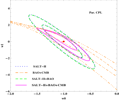
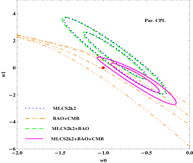
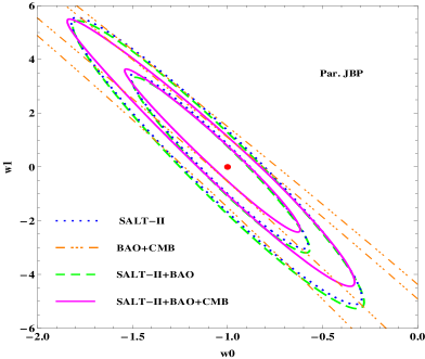
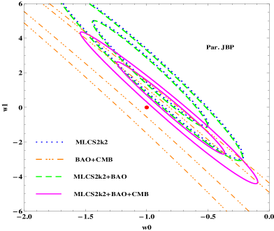
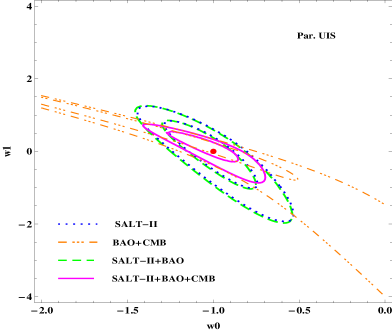
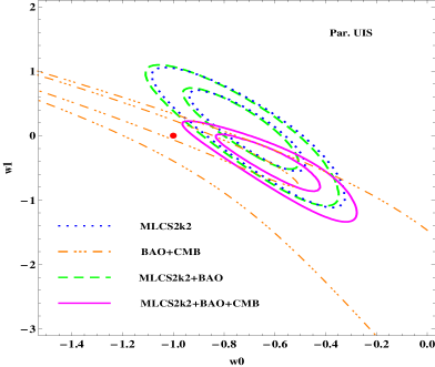
Figure 1: The $68.3\%$ and $95\%$ confidence level regions for $w_{0}$ versus $w_{1}$. The blue dotted, yellow dot-dashed, green dashed and pink solid lines represent the results obtained from SNIa, BAO+CMB, SNIa+BAO and SNIa+BAO+CMB, respectively. The left panels show the results obtained from SNIa with SALT fit, while the right panels are the results from SNIa with MLCS2k2 fit. The red point at $w_{0}=-1$, $w_{1}=0$ represents the spatially flat $\Lambda$CDM model.

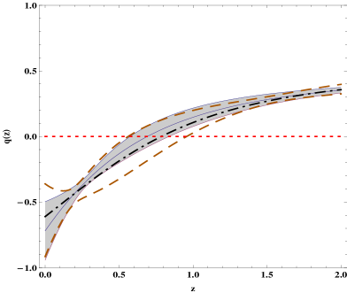
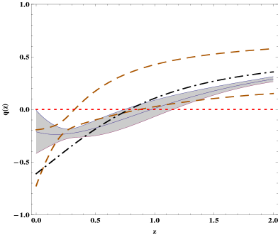
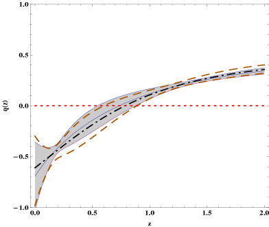
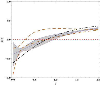
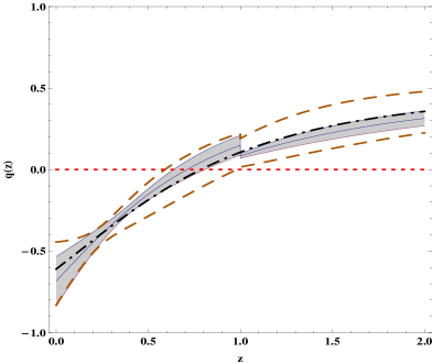
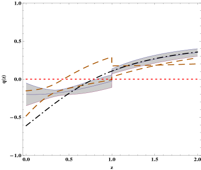
Figure 2: The gray regions and the regions between two dashed lines show the evolutionary behaviors of $q(z)$ at the $68.3\%$ confidence level obtained from SNIa+BAO+CMB and SNIa+BAO, respectively. The left panels show the results obtained from SNIa with SALT fit, while the right panels are the results from SNIa with MLCS2k2 fit. The dot-dashed lines represent the best-fit spatially flat $\Lambda$CDM model.

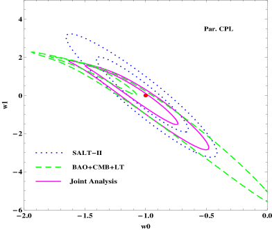
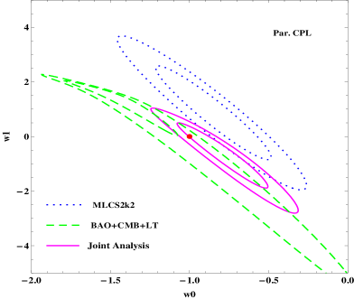
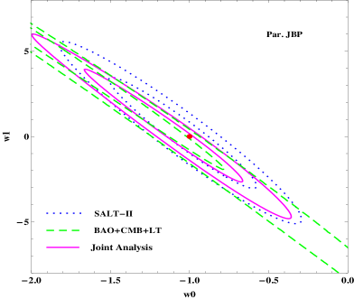
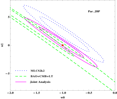
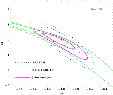
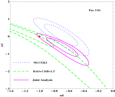
Figure 4: The $68.3\%$ and $95\%$ confidence level regions for $w_{0}$ versus $w_{1}$. The blue dotted, green dashed and pink solid lines represent the results obtained from SNIa, BAO+CMB+LT and SNIa+BAO+CMB+LT, respectively. The left panels show the results obtained from SNIa with SALT fit, while the right panels are the results from SNIa with MLCS2k2 fit. The red point at $w_{0}=-1$, $w_{1}=0$ represents the spatially flat $\Lambda$CDM model.

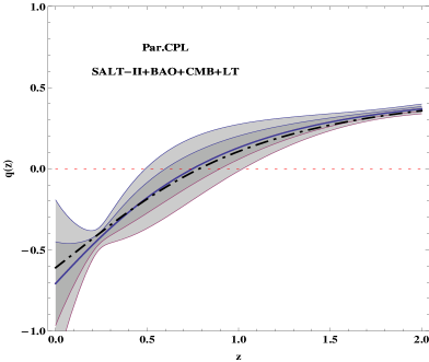
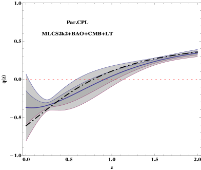
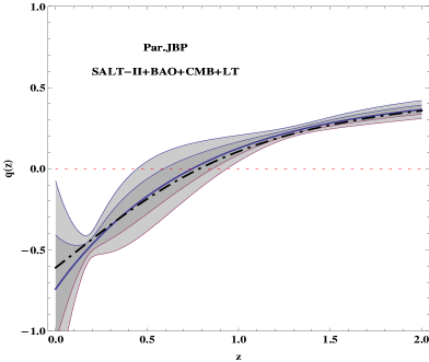
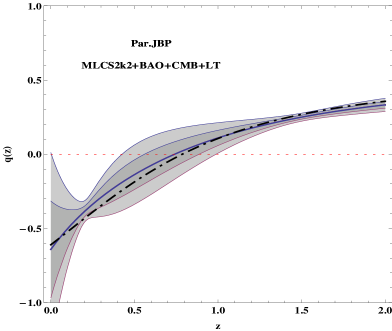
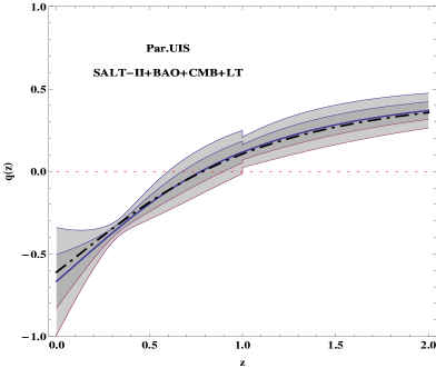
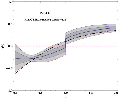
Figure 5: The gray regions show the evolutionary behaviors of $q(z)$ at the $68.3\%$ and $95\%$ confidence levels obtained from SNIa+BAO+CMB+LT. The dot-dashed lines represent the best-fit spatially flat $\Lambda$CDM model. The left panels show the results obtained from SNIa with SALT fit, while the right panels are the results from SNIa with MLCS2k2 fit.

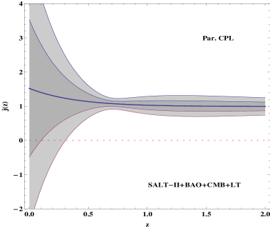
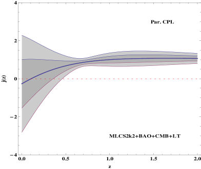
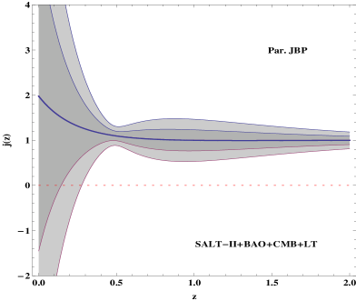
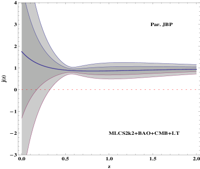
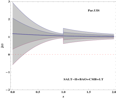
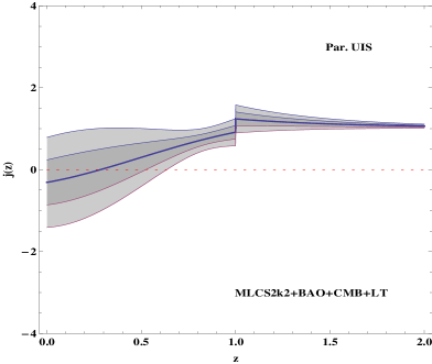
Figure 6: The gray regions show the evolutionary behaviors of $j(z)$ at the $68.3\%$ and $95\%$ confidence levels obtained from SNIa+BAO+CMB+LT. The left panels show the results obtained from SNIa with SALT fit, while the right panels are the results from SNIa with MLCS2k2 fit.

References

- (1) A. G.Riess, et al., Astron. J. 116, 1009 (1998).
- (2) S. Perlmutter, et al., Astrophy. J. 517, 565 (1999).
- (3) G. Hinshaw, et al., Astrophys. J. Suppl. Ser. 180, 225 (2009); E. Kommatsu, et al., Astrophys. J. Suppl. Ser. 180, 230 (2009).
- (4) A. Vikhlinin, et al., Astrophys. J. 692, 1060 (2009).
- (5) E. Rozo, et al., Astrophys. J. 708, 645 (2010).
- (6) U. Alam, V. Sahni, T. D. Saini, A. A. Starobinsky, Mon. Not. Roy. Astron. Soc. 354, 275 (2004); U. Alam, V. Sahni, A. A. Starobinsky, J. Cosmol. Astropart. P. 0406, 008 (2004); Y. Wang and P. Mukherjee, Astrophys. J. 606, 654 (2004); R. Lazkoz, S. Nesseris and L. Perivolaropoulos, J. Cosmol. Astropart. P. 0511, 010 (2005); S. Nesseris and L. Perivolaropoulos, J. Cosmol. Astropart. P. 0701, 018 (2007); P. Wu and H. Yu, Phys. Lett. B 643, 315 (2006)
- (7) Y. G. Gong and A. Wang, Phys. Rev. D 75, 043520 (2007); Y. G. Gong, R. G. Cai, Y. Chen and Z. H. Zhu, J. Cosmol. Astropart. Phys. 01, 019 (2010).
- (8) M. Chevallier and D. Polarski, Int. J. Mod. Phys. D 10, 213 (2001); E. V. Linder, Phys. Rev. Lett. 90, 091301 (2003).
- (9) H. K. Jassal, J. S. Bagla, and T. Padmanabhan, Mon. Not. R. Astron. Soc. 356, L11 (2005); T. Roy Choudhary and T. Padmanabhan, Astron. Astrophys. 429, 807 (2005).
- (10) A. Upadhye, M. Ishak, ahd P. Steinhardt, Phys. Rev. D 72, 063501 (2005).
- (11) V. Sahni, A. Shafieloo and A. A. Starobinsky, Phys. Rev. D 78, 103502 (2008).
- (12) M. Hicken, et al., Asrophys. J. 700, 1097 (2009).
- (13) W. J. Percival, et al., Mon. Not. R. Astron. Soc. 381, 1053 (2007).
- (14) B. A. Reid, arXiv: 0907.1659; W. J. Percival, et al., arXiv: 0907.1660.
- (15) A. Shafieloo, V. Sahni and A. A. Starobinsky, Phys. Rev. D 80, 101301 (2009).
- (16) Y. G. Gong, B. Wang, R. G. Cai, J. Cosmol. Astropart. Phys. 04, 019 (2010).
- (17) R. Kessler, et al., Astrophys. J. Suppl. Ser. 185, 32 (2009).
- (18) J. A. Frieman, et al., Astron. J. 135, 338 (2008).
- (19) M. Sako, et al., Astron. J. 135, 348 (2008).
- (20) W. M. Wood-Vasey, et al., Astrophys. J. 666, 694 (2007) .
- (21) S. Astier, et al., A&A, 447, 31 (2006).
- (22) A. G. Riess, et al., Astron. J. 116, 1009 (1998).
- (23) S. Jha, A. G. Riess, & R. P. Kirshner, Astrophys. J. 659, 122 (2007).
- (24) J. Simon, L. Verde and J. Jimenez, Phys. Rev. D 71, 123001 (2005).
- (25) S. Capozziello, et al., Phys. Rev. D 70, 123501 (2004); N. Pires, Z.-H. Zhu and J. S. Alcaniz, Phys. Rev. D 73, 123530 (2006).
- (26) M. A. Dantas, J. S. Alcaniz, D. Jain, A.Dev, Astron. Astrophys. 467, 421 (2007).
- (27) E. Komatsu, et al., arXiv:1001.4538v2
- (28) J. C. Bueno Sanchez, S. Nesseris and L. Perivolaropoulos, arXiv:0908.2636.
- (29) S. Nesseris and L. Perivolaropoulos, Phys. Rev. D 72, 123519 (2005).
- (30) H. K. Jassal, J. S. Bagla and T. Padmanabhan, Mon. Not. Roy. Astron. Soc. 405, 2639 (2010) [arXiv: astro-ph/0601389]
- (31) H. K. Jassal, J. S. Bagla and T. Padmanabhan, Phys. Rev. D 72, 103503 (2005).