Modeling CO Emission: I. CO as a Column Density Tracer and the X-Factor in Molecular Clouds

Abstract

Theoretical and observational investigations have indicated that the abundance of carbon monoxide (CO) is very sensitive to intrinsic properties of the gaseous medium, such as density, metallicity, and the background radiation field. CO observations are often employed to study the properties of molecular clouds (MCs), such as mass, morphology, and kinematics. It is thus important to understand how well CO traces the total mass, which in MCs is predominantly due to molecular hydrogen (H₂). Recent hydrodynamic simulations by Glover & Mac Low have explicitly followed the formation and destruction of molecules in model MCs under varying conditions. These models have confirmed that CO formation strongly depends on the cloud properties. Conversely, the formation of H₂ is primarily determined by the amount of time available for its formation. We apply radiative transfer calculations to these MC models in order to investigate the properties of CO line emission. We focus on integrated CO (J=1-0) intensities emerging from individual clouds, including its relationship to the total, H₂, and CO column densities, as well as the “$X$ factor,” the ratio of H₂ column density to CO intensity. Models with high CO abundances have a threshold CO intensity $\approx$65 K km s^-1 at sufficiently large extinctions (or column densities). Clouds with low CO abundances show no such intensity thresholds. The distribution of total and H₂ column densities are well described as log-normal functions, though the distributions of CO intensities and column densities are usually not log-normal. In general, the probability distribution functions of the integrated intensity do not follow the distribution functions of CO column densities. In the model with Milky Way-like conditions, the $X$ factor is in agreement with the near constant value determined from observations. In clouds with lower metallicity, lower density, or a higher background UV radiation field, the CO abundances are in general lower, and hence the $X$ factor can vary appreciably - sometimes by up to 4 orders of magnitude. In models with high densities, the CO line is fully saturated, so that the $X$ factor is directly proportional to the molecular column density.

1 Introduction

Since stars form almost exclusively in clouds which are predominantly molecular, much effort in current star formation research is focused on understanding the physics and chemistry of molecular clouds (MCs). Though MCs are primarily composed of molecular hydrogen (H₂), due to the lack of a dipole moment and the unsuitable conditions within MCs to excite its rotational transitions, H₂ is difficult to observe directly. Helium, accounting for $\approx 10\%$ of the cloud mass, is also very difficult to detect. Carbon monoxide (CO), which is the second most abundant molecular species in MCs, has a dipole moment with rotational transitions that are easily excited at typical MC temperatures (10 - 100 K) and densities ( $\buildrel>\over{\sim}$ 100 cm^-3). CO observations are thus often employed to investigate MC properties.

The observed CO intensity, $I$(CO), which is often expressed as a integrated “brightness temperature” $W_{\rm CO}$ (hereafter $W$), is considered to be a good tracer of the column density of molecular hydrogen $N_{\rm H_{2}}$. Namely, $N_{\rm H_{2}}$ is estimated from CO observations through a constant “$X$ factor” (e.g. Dickman, 1978):

$$X=\frac{N_{\rm H_{2}}}{W}\,({\rm cm}^{-2}\,{\rm K}^{-1}\,{\rm km}^{-1}\,{\rm s}).$$ (1)

CO observations of Galactic clouds have resulted in estimates of $X$ $\approx$ few $\times 10^{20}$ cm^-2 K^-1 km^-1 s (hereafter $X_{\rm Gal}$, e.g. Solomon et al., 1987; Young & Scoville, 1991; Dame et al., 2001). Observations of diffuse gas in the Galaxy have also resulted in similar estimates of the $X$ factor (e.g. Polk et al., 1988; Liszt et al., 2010).

However, extragalactic observations of systems with different physical characteristics, such as metallicity or background UV radiation, have found variations in the $X$ factor. Interestingly, observational investigations employing different methodologies have resulted in vastly discrepant estimates of the $X$ factor. For example, for the nearby Small Magellanic Cloud (SMC), Bolatto et al. (2008) measure a value $\approx$$X_{\rm Gal}$, assuming virialized clouds and using the CO linewidths to estimate cloud masses, and thereby $N_{\rm H_{2}}$. Independent dust and gas based observations, on the other hand, suggest extended regions containing molecular material with little or no CO emission, resulting in an $X$ factor of up to $\sim$100$X_{\rm Gal}$ (Israel, 1997; Rubio et al., 2004; Leroy et al., 2007; Leroy et al., 2009).

The ¹²CO (J=1-0) line is optically thick in most molecular clouds, and so CO (J=1-0) observations are known not to provide direct information about the total CO mass or column density $N_{\rm CO}$. Observations have shown a saturation of CO intensities at sufficiently high extinctions (e.g. Lombardi et al., 2006; Pineda et al., 2008). Consequently, only CO intensities below the saturation threshold are considered in evaluations of the $X$ factor. One of the goals of this work is therefore to assess how well CO observations can trace the true CO distribution within molecular clouds.

Since the formation of CO is sensitive to the amount of carbon and oxygen available in the ISM, CO abundances are expected to be lower in lower metallicity systems (Maloney & Black, 1988; Israel, 1997). Additionally, the strength of the background ultraviolet (UV) radiation field, responsible for photodissociating molecules, also plays a role in regulating the CO abundances (van Dishoeck & Black, 1988). These processes should in turn lead to variations in the $X$ factor, with a larger value in metal poor systems and/or where the UV radiation is higher than in the Milky Way. Indeed, when independent measures of MC masses are combined with CO observations, the $X$ factor has been found to be larger in low metallicity external galaxies, such as the LMC and SMC (Israel et al., 1986; Israel, 1997; Leroy et al., 2009).

As turbulence is now considered an important aspect of the dynamics in molecular clouds and star formation (Mac Low & Klessen, 2004; Ballesteros-Paredes et al., 2007; McKee & Ostriker, 2007, and references therein), its role in influencing molecule formation needs to be understood. Glover & Mac Low (2007b) (see also Glover & Mac Low, 2007a), showed that the formation timescale of H₂ is only a few Myr in turbulent MC models with densities comparable to those in observed clouds. Expanding on this work, through implementation of more extensive chemistry, we can now follow the formation of CO in models of turbulent molecular clouds (Glover et al., 2010, hereafter Paper I). Subsequently, Glover & Mac Low (2010), hereafter Paper II, analysed the global properties of the $X$ factor in different MC models, using spatially averaged quantities. They found that the mean extinction, or total gas column density, primarily determines the $X$ factor.

Here, we explore the observational consequences of the variation in CO abundances which arise due to differences in MC properties described in Papers I-II. Our main goal is to understand the impact of CO abundance variations within individual MCs on the emerging integrated CO (J=1-0) intensity. We consider a suite of models with different conditions, namely metallicity, density, and background UV radiation field, representing various environments. In the next section we discuss our modeling method, including a brief overview of the magnetohydrodynamic models with chemistry, and a description of the radiative transfer calculations. In Section 3 we present our results of the comparison of CO intensities with H₂ and CO column densities, and characteristics of the the $X$ factor. We discuss our results and compare them to observational investigations in Section 4. We conclude with a summary in Section 5.

2 Modeling Method

To carry out our investigation of CO emission from molecular clouds, we apply line radiative transfer calculations to magneto-hydrodynamic (MHD) models of MCs. In this section, we give a brief description of the MHD models, and focus on the radiative transfer calculations. We refer the reader to Papers I and II for a more extensive description of the MHD and chemical modeling method, as well as the analysis of various simulation runs.

2.1 Modeling Molecular Clouds: MHD and Chemistry

The simulations of the model MCs track the evolution of gas using a modified version of the ZEUS-MP MHD code (Norman, 2000; Stone & Norman, 1992a, b). Gas with initially uniform density in a 20 pc box with periodic boundary conditions is driven with a turbulent velocity field, with uniform power between wavenumbers $1\leq k\leq 2$. Gas self-gravity, which would cause sufficiently overdense regions to collapse, is not considered in the calculation. The simulation includes magnetic fields, with initial field lines oriented parallel to the $\hat{z}$-axis with a field strength of 1.95 $\mu$G. The gas has an initial temperature of 60 K, but quickly settles to thermal equilibrium.

To track the chemical evolution of the gas, which has constant metallicity, a treatment of hydrogen, oxygen, and carbon chemistry is included in the numerical algorithm. This consists of 218 reactions of 32 chemical species, which are coupled with the thermodynamics. A background UV radiation field, which is responsible for photodissociation, is treated through the six-ray approximation as described in Glover & Mac Low (2007a). In our investigation of emission from CO molecules, we consider one snapshot of these simulations at a late time $>$ 5 Myr, after which the simulation has reached a statistically steady state.

2.1.1 GMC Model Parameters

The numerical modeling described above follows the combined effects of turbulence, magnetic fields, thermodynamics, and chemical evolution as structures such as filaments and dense cores typically found in MCs forms out of the gas (see Paper I for more details). In our investigation of CO emission emerging from the MC simulations, we consider a suit of models designed to represent various astrophysical environments. The relevant parameters of each model are listed in Table 1. Column 1 shows the name of each run. The main user defined parameters are the initial density $n_{0}$, metallicity $Z$, and background UV radiation field $G_{0}$, indicated in Columns 2-4, respectively. We assume that the dust-to-gas ratio is directly proportional to the gas-phase metallicity and do not vary these quantities independently. Column 5 shows the numerical resolution; as noted in Paper II, simulations with identical initial conditions but resolutions of 256³ and 128³ produce very similar results. The last column lists the representative environment corresponding to the simulated cloud: a high density cloud found in the galactic center (n1000), a typical Milky Way cloud (n300, Ferrière, 2001), clouds in low metallicity systems like the LMC or SMC (n300-Z03 and n300-Z01), a low density cloud in a dwarf galaxy (n100), and clouds in weak and strong starbursts (n300-UV10 and n300-UV100, respectively).

Table 1: List of Simulations

ID	$n_{0}$ (cm-3)	Z	G0 (2.7$\times 10^{-3}$ erg cm-2 s-1 )	Resolution	Representative Environment
n1000	1000	1.0	1.0	1283	high-density cloud (galactic center)
n300	300	1.0	1.0	2563	Milky Way cloud
n300-Z03	300	0.3	1.0	2563	LMC/SMC cloud
n300-Z01	300	0.1	1.0	2563	LMC/SMC cloud
n100	100	1.0	1.0	2563	dwarf galaxy cloud
n300-UV10	300	1.0	10.0	1283	weak starburst
n300-UV100	300	1.0	100.0	1283	strong starburst

2.2 Radiative Transfer Method

2.2.1 Radiative Transfer Overview

We use the radiative transfer code RADMC-3D (Dullemond et al. in preparation) to model the molecular line emission of the MHD MC models. RADMC-3D is a 3-dimensional code that performs dust and/or line radiative transfer on Cartesian or spherical grids (including adaptive mesh refinement). In this work, since we are only interested in CO molecular line emission along a chosen direction, we use the ray tracing capability of RADMC-3D.

One of the primary challenges in line radiative transfer is to solve for the population levels of the molecular (or atomic) species under consideration. The occupation of a given (rotational/vibrational) energy level of a molecule depends on the incident radiation field, as well as the collision properties (e.g. frequency) with other atoms or molecules, both of which act as excitation or de-excitation mechanisms. In statistical equilibrium, the relative population of level $i$, $f_{i}$, is governed by the equation of detailed balance:

$$\sum_{j>i}[{f_{j}A_{ji}+(f_{j}B_{ji}-f_{i}B_{ij})\bar{J}_{ji}}]-$$

$$\sum_{j<i}[{f_{i}A_{ij}+(f_{i}B_{ij}-f_{j}B_{ji})\bar{J}_{ij}}]+$$

$$\sum_{j}[{f_{j}C_{ji}-f_{i}C_{ij}}]=0$$ (2)

The last summation accounts for collisions, where $C_{ij}$ is the collisional rate for a transition from level $i$ to level $j$. The collisional rate is dependent on the rate coefficient $K_{ij}$ and the density of the collisional partner $n_{col}$: $C_{ij}=n_{col}K_{ij}$. In MCs, the main collisional partner of CO is H₂. We use the rate coefficients for collisional excitation and de-excitations of CO by H₂ tabulated and freely available from the Leiden database (Schöier et al., 2005). These are based on calculations by Yang et al. (2010). We neglect the effect of collisions with partners other than H₂. We justify this by noting that almost all of the CO in our simulations is found in regions of the gas that are dominated by H₂, rather than atomic hydrogen.

The influence of radiation on setting the level populations is captured by the first two summations in Equation 2, which include the mean integrated intensity $\bar{J}_{ij}$ of the radiation field in the line corresponding to the transition from $i$ to $j$. The constants are $A_{ij}$, the Einstein coefficient for spontaneous emission for a transition from level $i$ to level $j$, $B_{ij}$, the Einstein coefficient for stimulated emission from $i$ to level $j$, and $B_{ji}$, the corresponding coefficient for absorption (also given by the Leiden database). Equation 2 is coupled with the equation of radiative transfer

$$\frac{dI_{\nu}}{d\tau_{\nu}}=-I_{\nu}+S_{\nu},$$ (3)

where $I_{\nu}$ is the specific intensity, $S_{\nu}$ the source function, and $\tau_{\nu}$ is the optical depth. The coupling between Equations 2 and 3 occurs through the dependence of the source function ($S_{\nu}=S_{ij}$) on the relative population levels:

$$S_{ij}=\frac{f_{i}A_{ij}}{f_{j}B_{ji}-f_{i}B_{ij}},$$ (4)

as well as the dependence of the $\bar{J}$ on $I$:

$$\bar{J}_{ij}=\frac{1}{4\pi}\int I_{ij}\phi_{ij}d\Omega,$$ (5)

where the integral is taken over all solid angles $\Omega$. The normalized profile function $\phi_{ij}$ determines the emission and absorbtion probability of a photon with frequency $\nu$, due to a line with rest frequency $\nu_{ij}$. For a photon propagating in a direction ${\bf\hat{n}}$ through a medium with velocity ${\bf v}$,

$$\phi_{ij}(\nu)=\frac{c}{a\nu_{ij}\sqrt{\pi}}\exp\left(-\frac{c^{2}(\nu-\nu_{ij}-{\bf v}\cdot{\bf\hat{n}}\nu_{ij}/c)^{2}}{a^{2}\nu_{ij}^{2}}\right),$$ (6)

where $c$ is the light speed. The thermal and microturbulent broadening of the line is accounted for through

$$a^{2}=v_{mtrb}^{2}+2k_{B}T/m_{mol},$$ (7)

where $k_{B}$ is the Boltzmann constant, $m_{mol}$ is the molecular (or in the case of atomic lines, atomic) mass, $T$ is the temperature, and $v_{mtrb}$ is the microturbulent velocity of the medium.

As Equations 2 - 5 indicate, the amount of radiation emitted from molecules in a given location is dependent on the level populations, which themselves depend on the amount of incident radiation at that location. Solving this problem numerically can be computationally expensive. In certain situations, however, suitable approximations can be made which considerably reduce the computational costs.

One approximation is that of local thermodynamic equilibrium (LTE). In gaseous systems, when collisional processes dominate line emission, the temperature is the only parameter that is required to calculate the population levels, through the use of a partition function. Thus, in regions with high H₂ densities, employing the LTE assumption to model the CO (J=1-0) line is reasonable. However, in the MC environments considered here, much of the volume does not contain high densities, so the LTE approximation may not be suitable.

2.2.2 The Sobolev approximation

For this study, we have implemented the Sobolev approximation (Sobolev 1957; also known as the Large Velocity Gradient, or LVG, method) into RADMC-3D to solve for the population levels of an atomic or molecular species. This method takes advantage of large spatial variations in velocity, as are present in turbulent molecular clouds, to define line escape probabilities. Effectively, the LVG method provides a solution to the equation of detailed balance (Eqn. 2) determined solely by local quantities.

Consider a photon emitted due to a transition from level $i$ to level $j$. Beyond a certain distance from the photon’s position of emission, due to the velocity gradient in the medium, the Doppler-shifted frequency associated with the $i$ to $j$ transition is sufficiently different from that of the incident photon. The photon cannot interact with matter at this position, or any subsequent position, and thus propagates freely out of the cloud. The LVG escape probability of the photon can be determined from the optical depth

$$\beta=\frac{1}{\tau}\int_{0}^{\tau}e^{-\tau^{\prime}}d\tau^{\prime}=\frac{1-e^{-\tau}}{\tau}.$$ (8)

Other functional forms of the escape probability can be defined for different scenarios (e.g. slab or spherical symmetry, see van der Tak et al., 2007). The optical depth is determined by the population levels, densities, and velocity gradients $dv/dr$ (van der Tak et al., 2007):

$$\tau=\frac{c^{3}}{8\pi\nu_{ij}^{3}}\frac{A_{ij}n}{1.065<|dv/dr|>}\left(f_{j}\frac{g_{i}}{g_{j}}-f_{i}\right)$$ (9)

where $g_{i}$ is the statistical weight of level $i$, and $n$ is the total density of the molecular species ($f_{i}$ is the relative population, so that $\sum_{i}f_{i}=1$). We use the mean (absolute) velocity gradient $<|dv/dr|>$ across the six faces of each grid zone in the simulation. The near unity factor in the denominator is a correction for integration over a Gaussian line profile.

Once the optical depth is computed, the escape probability is given by Equation 8. The local radiation field is then determined by

$$\bar{J_{ij}}=S_{ij}(1-\beta)$$ (10)

Numerically, given these expressions for $\tau$, $\beta$, $\bar{J}$, and the local velocity gradient, one can iteratively solve for the population levels in Equation 2; for more detailed descriptions of the LVG method see Mihalas (1978) and Elitzur (1992).

Though the LVG method was originally formulated and developed for spectral line studies in stellar atmospheres which have smooth velocity gradients (Sobolev, 1957; Castor, 1970; Mihalas, 1978), it can also be applied for any environments with significant velocity gradients. In fact, Ossenkopf (1997) showed that the Sobolov method is a very good approximation for computing level populations in MCs, where the velocity gradients are generally not smooth.

2.3 Analysis of CO Emission

In this work, we focus on how well CO emission can trace the intrinsic CO column density, $N_{\rm CO}$, the H₂ column density $N_{\rm H_{2}}$, as well as the total column density of hydrogen nuclei, $N_{\rm tot}$. The intrinsic column densities can be easily calculated directly from the MHD simulation by integrating the CO, H₂ and hydrogen nuclei volume densities along a given axis. Accordingly, for the radiative transfer calculation we orient the simulation cube such that the CO line is “observed” along the same axis for which the column densities are computed (e.g. along the $\hat{z}$-axis). We have verified that our results are not sensitive to the choice of orientation.

Besides the viewing geometry, the only other user defined parameter required for the radiation transfer calculations is the microturbulent velocity $v_{mtrb}$ [see Eqns. 6-7]. Extrapolating the observed linewidth-size relationship (e.g. Larson, 1981) down to the resolution of the MHD simulations $\sim$ 0.1 pc, appropriate microturbulent velocities are in the range $\sim$ 0.2 - 0.7 km s^-1. We have explored this range in $v_{mtrb}$, and have found that the results are insensitive to the particular choice of $v_{mtrb}$. In the analysis presented here, $v_{mtrb}$ is set to 0.5 km s^-1.

In our discussion, we will sometimes express $N_{\rm tot}$ as an extinction $A_{V}$, in order to allow for direct comparison with observational analyses. Observers are often required to employ indirect measures of $N_{\rm tot}$, since H₂, a major constituent of $N_{\rm tot}$ in MCs, is difficult to observe directly. Extinction measurements provide estimates of the total amount of dust along the line of sight. Using a “reddening law,” (and an assumption for the dust-to-gas ratio), the total gaseous column follows directly from the amount of extinction $A_{V}$ (Bohlin et al., 1978). In many Galactic molecular clouds, nearly all the hydrogen is molecular, so $N_{\rm H_{2}}$ is directly proportional to $A_{V}$. In other environments, however, such as those with lower metallicity or higher UV fields (e.g. Models n300-Z01 and n300-UV2), there may be significant amounts of atomic hydrogen, so $N_{\rm tot}$, and hence the extinction, is dependent on both the molecular and atomic column densities. To allow for straightforward comparison between models and observations, we use a simple conversion between $N_{\rm tot}$ and $A_{V}$:

$$A_{V}=\frac{N_{\rm tot}}{1.87\times 10^{21}\,{\rm cm}^{-2}}\>\left(\frac{\rm Z}{\rm Z_{\odot}}\right),$$ (11)

where ${\rm Z}$ is the metallicity of the gas. Thus, in the comparison of CO emission with intrinsic cloud properties, any discussion involving $A_{V}$ can be directly translated into total column density.

The radiative transfer calculations produce spectral (position-position-velocity, or PPV) cubes of the CO (J=1-0) line. The 3D cube indicates the intensity $I_{\nu}$ in a given frequency or velocity channel of width $dv$ at each 2D position. We choose a sufficiently large range in frequencies such that all (line-of-sight) velocities in the simulation are detected, so that all emission from the model MC is “observed.”

In the comparison of CO intensities with intrinsic column densities, as well as the analysis of the $X$ factor, the quantity of interest is the velocity integrated intensity, which is simply the PPV cube integrated over its velocity axis. The intensity $I_{\nu}$, which has units of erg s^-1 cm^-2 Hz^-1 ster^-1, can be expressed as the Planck function evaluated at a “brightness temperature” $T_{B}$, $B_{\nu}(T_{B})$. Since the CO (J=1-0) line is located in the Rayleigh-Jeans part of the spectrum, $I_{\nu}\propto T_{B}$. The intensity of CO line emission is thus often conveyed in $T_{B}$ units. We follow this convention and express the intensity as a velocity integrated brightness temperature:

$$W=\frac{1}{2k_{B}}(c/\nu)^{2}\int I_{\nu}dv\,\,({\rm K\,km\,s^{-1}}).$$ (12)

This integrated intensity is thus a measure of total CO emission along the line of sight. $W$ is computed at all positions yielding a 2D map, which can be used with the 2D map of $N_{\rm H_{2}}$ to obtain the $X$ factor through Equation 1.

3 Results

3.1 CO Intensities and Column Densities

To begin our investigation of CO emission, we assess the correlation of velocity integrated CO intensities $W$ with the total column density $N_{\rm tot}$ of the model MCs. Figure 1 shows $W$ as a function of the $N_{\rm tot}$ for four of the simulations listed in Table 1. The bottom abscissa shows $N_{\rm tot}$, while the top abscissa shows the corresponding $A_{V}$ (see Eqn. 11).

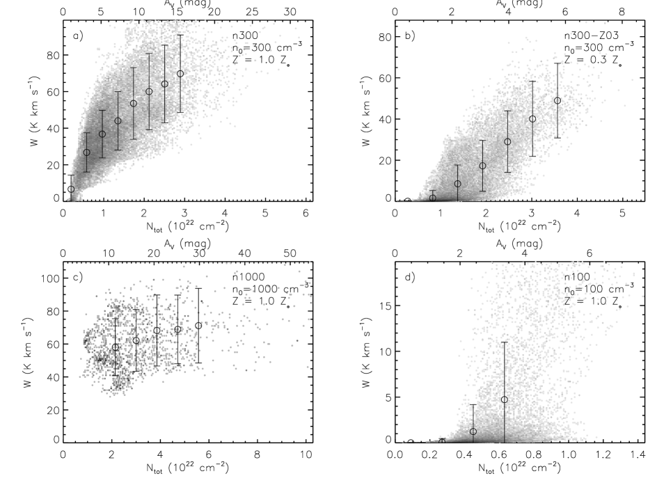
Figure 1: Relationship between integrated CO intensity $W$ and total column density $N_{\rm tot}$ (bottom abscissa) or extinction $A_{V}$ (top abscissa) for four models: a) n300, b) n300-Z03, c) n1000, and d) n100. The color of each point indicates the frequency of a given $A_{V}$ and $W$ pair, with darker points corresponding to higher frequencies. Circles show average $W$ values in $A_{V}$ bins, and the error bars indicate 1$\sigma$ deviations.

A number of features are readily apparent in Figure 1. First, there is a general trend of increasing intensity with increasing column density, though the slopes differ between the various simulations. For the high-density run (n1000) shown in Figure 1c, the CO intensities do not demonstrate any clear trend with increasing $A_{V}$. Rather, the vast majority of the intensities reach a threshold value of $\sim$65 K km s^-1. This saturation of CO intensities is expected to occur at high densities since the CO line becomes optically thick. Saturation is also found at the highest extinctions in the Milky Way simulation (n300, Fig 1a). Indeed, saturation at high CO intensities has been observed in MCs in the solar neighborhood (e.g. Lombardi et al., 2006; Pineda et al., 2008). Though model n300 qualitatively reproduces the observed trends of increasing CO intensity with increasing density, up to a threshold value, a detailed quantitive comparison is not appropriate here; the precise slope, scatter, minimum, and threshold intensity are dependent on additional physics not included in our models, such as additional heating due to stars, outflows, and supernovae.

Figure 1b and d show that for clouds with lower metallicities (Model n300-Z03) or densities (Model n100), there is a wider distribution of CO intensities at low extinctions. The saturation of the CO line is not easily evident compared to Model n1000. Since CO is easily photo-dissociated in low metallicity or low density systems due to insufficient (dust and self-) shielding, the CO column densities do not reach high enough values for the saturation of the CO line to occur. Observations have indeed shown that the CO intensities are generally lower in extragalactic systems with lower metallicities than that of the Milky Way. Further, there is no evidence of saturation in the CO line from diffuse sources such as the Polaris Flare, LMC and SMC (e.g. Heithausen et al., 1993; Israel, 1997; Leroy et al., 2009).

Figure 2 shows the probability distribution functions (PDFs) of $N_{\rm tot}$ (or $A_{V}$), $N_{\rm H_{2}}$, $N_{\rm CO}$, and $W$ for five models. The $N_{\rm tot}$ PDFs are offset to larger values compared with the $N_{\rm H_{2}}$ PDFs. The offset for the Milky Way (n300) and the high density cloud (n1000) can be wholly attributed to the difference in $N_{\rm tot}$, which is a measure of the total number of hydrogen nuclei, and $N_{\rm H_{2}}$, a measure of the number of molecular hydrogen nuclei. For the other models, there remains an offset even after accounting for the factor of 2 difference between $N_{\rm tot}$ and $N_{\rm H_{2}}$, because significant amounts hydrogen remains in atomic form (see Table 2 of Paper II).

Figure 2: PDFs of left: molecular hydrogen column density $N_{\rm H_{2}}$ (thin) and total column density $N_{\rm tot}$ (thick), right: CO column density $N_{\rm CO}$ (thin) and integrated CO intensity $W$ (thick) from five models. In the panels on the left, the bottom abscissas indicate column density, and top abscissas indicate total extinction. In the panels on the right, the bottom abscissas indicate $N_{\rm CO}$ values, and top abscissas indicate $W$ values. For Model n300-Z03 (c-d), solid lines mark log($N_{\rm CO}$)=12, 14 and log($W$)=-3, -1 and dashed lines mark log($N_{\rm CO}$)=16.5 and log($W$)=1.5, for comparison with Figure 4 (see text). Best fit Gaussians are overplotted for Models n300 (a-b) and n1000 (e-f). Model parameters are indicated within each plot.

The $N_{\rm tot}$ and $N_{\rm H_{2}}$ PDFs of all simulations can be well described as log-normal functions. Log-normal column density PDFs should be expected from these compressible turbulent simulations (Vazquez-Semadeni, 1994; Klessen, 2000; Ostriker et al., 2001; Li et al., 2003; Federrath et al., 2010). The simulation with conditions similar to the Milky Way (n300) and with the highest density (n1000) produce $N_{\rm CO}$ and $W$ PDFs which come closest to being lognormal. In general, however, the CO column densities and intensities do not show a log-normal PDF. We defer the discussion of the best fit Gaussians shown for these two models to Section 4.1.

Another clear trend in Figure 2 is that the shapes of the $W$ PDFs can differ significantly from the PDFs of underlying $N_{\rm CO}$. The extent of the scales of $W$, shown on the top abscissas of the right hand plots in Figure 2, is equivalent to the extent of the scales in $N_{\rm CO}$, which appear on the bottom abscissas. At low densities where gas is optically thin, CO emission should trace the CO density. Thus, the absolute scales are chosen such that low $W$ and $N_{\rm CO}$ values are matched as best as possible. For models n300 (Figs 2a-b) and n1000 (Figs 2e-f) , the $W$ PDFs have steep increases, resulting in peaks that do not correspond to the peaks in the $N_{\rm CO}$ PDFs. The PDFs of the other simulations, n300-Z03, n300-Z01, and n100, show comparable gradients at low $W$ and $N_{\rm CO}$, but at high values the $W$ PDFs drop more rapidly than $N_{\rm CO}$.

In those PDFs showing a steep decline in $W$, at high CO column densities there is little or no corresponding CO emission, even though there is good correspondence at lower values (due in part to the choice of the $W$ and $N_{\rm CO}$ axis ranges). PDFs showing a much steeper gradient beyond the $W$ peak compared to the $N_{\rm CO}$ peak can be attributed to saturation of the CO line: as a result of saturation, regions with very high $N_{\rm CO}$ may have similar intensities to regions with lower (but still high) $N_{\rm CO}$, producing a PDF which appears to have a “piled-up” profile at some high $W$. Such PDF shapes are clearly evident in the moderately low metallicity (n300-Z03) and very low density (n100) cloud simulations. For the simulation with very low metallicity (n300-Z01) for which the $W$ and $N_{\rm CO}$ PDFs appear to be correlated, there is no evidence of a saturation feature.

We have shown that there is no simple correlation between $W$ and $N_{\rm CO}$, focusing on models with different metallicities and densities. Of course, the background radiation field also affects the formation of CO, due to UV photodissociation (van Dishoeck & Black, 1988, Paper II). Figure 3 shows the $N_{\rm H_{2}}$, $N_{\rm CO}$, and $W$ histograms from models n300, n300-UV10, and n300-UV100 (see Table 1). These models only differ in their background UV radiation field strengths, with values of G₀ = 1, 10, and 100 times the Galactic estimate (2.7$\times 10^{-3}$ erg cm^-2 s^-1). All simulations have similar log-normal $N_{\rm H_{2}}$ distributions. Simulations with higher UV fields have more extended $N_{\rm CO}$ PDFs, and thereby lowered maxima in the $N_{\rm CO}$ probabilities. This occurs because stronger UV radiation is able to penetrate further into the cloud to dissociate CO, resulting in more regions with low CO densities. Similarly, the $W$ distributions are more extended for models with brighter UV backgrounds, with fewer regions with high $W$ values. These results simply follow the trend previously discussed: models with a wide range in CO abundances demonstrate a lack of correlation between $W$ and $N_{\rm CO}$ PDFs. The lack of correlation in the PDFs primarily occur at the highest densities and intensities (with the exception of n300-Z01, but see last paragraph of this subsection), though at lower densities gas is optically thin resulting in a correlation between $W$ and $N_{\rm CO}$. Clouds with lower metallicity, lower overall density, higher UV background, or a combination of these factors have much more distributed CO abundances, resulting in greater discrepancies between the $W$ and $N_{\rm CO}$ PDFs. Keeping this general trend in mind, in our subsequent analysis we will focus on the models with G₀ = 1.

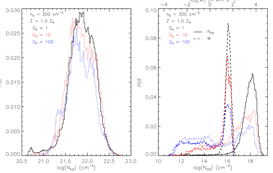
Figure 3: PDFs of left: $N_{\rm H_{2}}$, right: $N_{\rm CO}$ (solid thin) and $W$ (dashed thick) from three models with different background interstellar radiation fields (indicated within each plot). In the panel on the right, the bottom abscissa indicates $N_{\rm CO}$ values, and top abscissa indicates $W$ values.

We now turn our attention to the $W$ and $N_{\rm CO}$ properties of simulation n300-Z03 (Figs. 2c-d). There is a relatively large spread in $N_{\rm CO}$, which also has a clear double peak, at $\log(N_{\rm CO})\approx$ 14.5 and 16.5 (with similar probabilities). Further, though the $W$ PDF appears to correlate well with the $N_{\rm CO}$ PDF at low CO density (or low intensity) values, the peak in $W$ does not correlate well with the peak in $N_{\rm CO}$. A closer inspection of the $N_{\rm CO}$ and $W$ images for Model n300-Z03, shown in Figure 4a-b, further reveals the correlation at low densities, and lack of correlation at high densities. In the low intensity range $-3\leq$ log(W) $\leq\,-$1, marked by solid lines in Figure 2d, an increase in $W$ corresponds to a similar increase in $N_{\rm CO}$ in the 12 $\leq$ log($N_{\rm CO}$) $\leq$ 14 range. These $W$ and $N_{\rm CO}$ values are indicated by solid contours in Figure 4, showing excellent correspondence. However, at higher intensities, $W$ does not faithfully trace the high $N_{\rm CO}$ regions. The PDF of intensities at log($W$) $\geq$ 1.5, marked by a dashed line in Figure 2d, decreases sharply, whereas log($N_{\rm CO}$) continues to increase. The dashed contours in Figure 4 mark the corresponding regions in the $N_{\rm CO}$ and $W$ maps. In some of the filaments (e.g. near the bottom), the contours mark similar regions. However, in the most dense regions (e.g. the large over-dense region in the top right), the area within the $W$ contour is noticeably smaller than that encompassed in the $N_{\rm CO}$ map. The detailed morphology in the region encompassed by the dashed contour also shows stark differences between the observed CO intensities and intrinsic CO column densities. These differences at high densities are a direct consequence of the optically thick nature of the CO line.

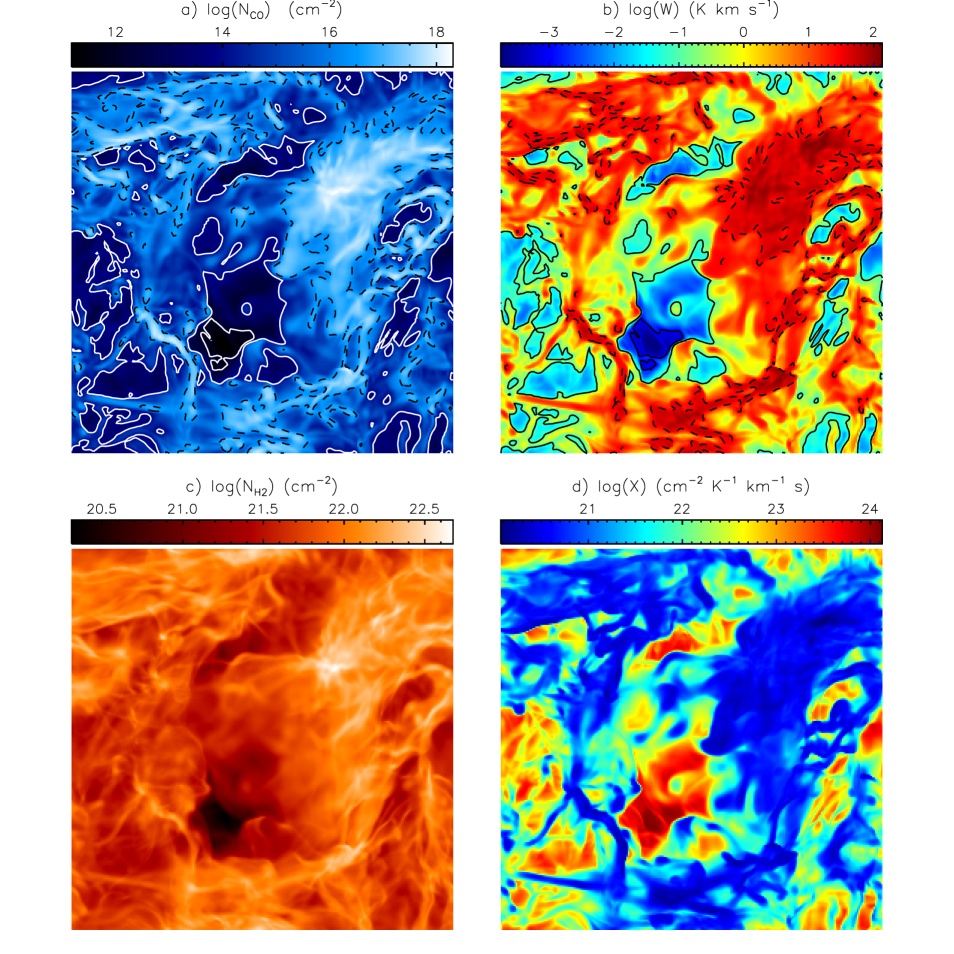
Figure 4: Images of a) $N_{\rm CO}$, b) $W$, c) $N_{\rm H_{2}}$, and d) the $X$ factor of Model n300-Z03. Each side has a length of 20 pc. In a) and b) solid contours indicate log($N_{\rm CO}$)=12, 14 and log($W$)=-3, -1; dashed contours are log($N_{\rm CO}$)=16.5 and log($W$)=1.5 (see text and Fig. 2d).

Similar discrepancies are present in a $N_{\rm CO}$ - $W$ comparison of all the models. In some cases, such as model cloud with very low metallicity, n300-Z01 shown in Figure 2j, the apparent correlation in PDFs at low densities does not translate into a correlation in the 2D maps. As stated, the $N_{\rm CO}$ and $W$ PDFs were plotted with abscissas chosen to best match the PDFs at low densities and intensities, and so any apparent correlation may only be coincidental.

In summary, we have shown that at low densities, CO emission traces the distribution of CO molecules well, since the CO line is optically thin. However, at high densities, the line becomes optically thick, resulting in an intensity threshold. Thus, CO intensity does not neatly trace the highest density gas. Further, there is generally no simple correlation in the distribution of CO and H₂ molecules, since H₂ can better shelf-shield against photodissociation. Taken together, the lack of any general correspondence between $W$ and $N_{\rm CO}$, as well as $N_{\rm CO}$ and $N_{\rm H_{2}}$, will certainly affect further analysis of CO observations, such as attempts at relating $W$ to $N_{\rm H_{2}}$.

3.2 The $X$ Factor

In Paper II, the $X$ factor (Eq. 1) from the models considered in this work was found to vary at low mean extinctions $\overline{A_{V}}$  $\buildrel<\over{\sim}$  3. At higher mean extinctions, the $X$ factor remained constant. In that work, the CO intensities were estimated by assuming local thermodynamic equilibrium (LTE), and by averaging relevant quantities over whole clouds. In the previous section, we demonstrated that CO observations do not neatly trace CO column density. A logical expectation from this result is that observed CO intensities would not be a good tracer of H₂ number density, leading to a variation in the $X$ factor as found in Paper II. In this section, we go beyond the analysis of Paper II to investigate the $X$ factor using the results from the 3D radiative transfer calculations to estimate CO line intensities. Here, we are also able to assess variations in the $X$ factor on a position-by-position basis in maps of the individual clouds.

Figure 5 shows the $X$ factor from each position in the 2D integrated intensity images of simulations n300, n300-Z03, n1000, and n100, along with the PDF of the $X$ factor. Each point indicates the relationship between $N_{\rm CO}$ and $N_{\rm H_{2}}$, and the color identifies its value of the $X$ factor, calculated from Equation 1.

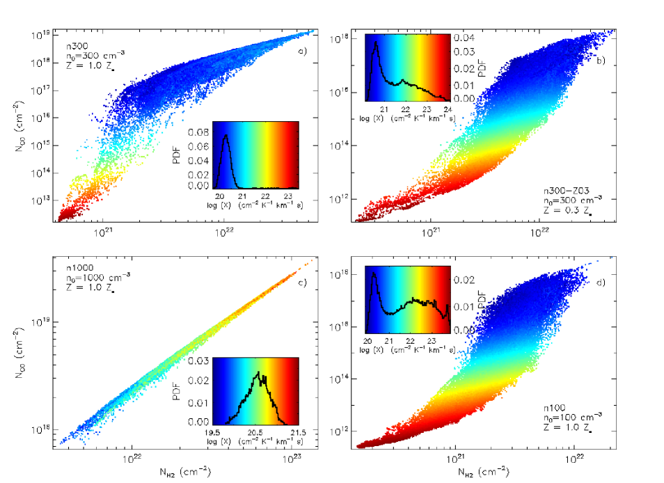
Figure 5: $X$ factor for four models. $N_{\rm CO}$ is plotted as a function of $N_{\rm H_{2}}$. The color of each point indicates the $X$ factor. Inset figures show the color scale and PDF of the $X$ factor. The corresponding maps of $N_{\rm H_{2}}$, $N_{\rm CO}$, and the $X$ factor from Model n300-Z03 are shown in Figure 4.

For the Milky Way MC model (n300, Fig. 5a), in $>$90% of positions the $X$ factor is within the range $9\times 10^{19}-5\times 10^{20}$ cm^-2 K^-1 km^-1 s. Figures 2a-b show that the quantities $N_{\rm H_{2}}$, $N_{\rm CO}$, and $W$ all have similar (Gaussian-like) shapes, which ultimately result in a limited range in the distribution of the $X$ factor. The range in the derived $X$ factor for this model is in agreement with estimates from observations of Milky Way clouds (e.g Solomon et al., 1987; Young & Scoville, 1991; Dame et al., 2001). This agreement gives us confidence that the simulations, including the chemical networks as well as the radiative transfer calculations, are sufficiently reliable and can be utilized to probe conditions different from the Milky Way.

The distribution of the $X$ factor increases substantially when the observed CO emission is poorly correlated with the CO column densities, as in Model n300-Z03 (Fig. 5b). In this model, the $X$ factor distribution spans a wide range: only $<$ 25% have values in the range $9\times 10^{19}-5\times 10^{20}$, and $>$30% have values $>10^{22}$ cm^-2 K^-1 km^-1 s.

Figure 4c and d shows $N_{\rm H_{2}}$ and the $X$ factor for each line-of-sight of Model n300-Z03. In the highest density regions such as the large complex at the top right-hand side of CO or H₂ column density maps (Figs. 4a and c), the $X$ factor has a limited range, within one order of magnitude ($10^{20}-10^{21}$ cm^-2 K^-1 km^-1 s). In those regions, though $N_{\rm CO}$ can vary by 2 or more orders of magnitude, $W$ only varies by $\approx$ 1 order of magnitude. Since the $X$ factor directly depends on $W$ and only indirectly on $N_{\rm CO}$, the $X$ factor also only falls into a limited range.

Positions with the largest $X$ factors correspond to the lowest $N_{\rm H_{2}}$ regions, as well as low $N_{\rm CO}$ and $W$ regions. These are the regions where CO is most affected by photodissociation. Since the amount of photodissociation depends on the the “effective” column density in each location of the 3D simulation volume, regions with similar $N_{\rm H_{2}}$ can have very different $N_{\rm CO}$ values (see also Paper I and II), as evident in Figure 5b: at low to intermediate H₂ densities $10^{21}$ $\buildrel<\over{\sim}$ $N_{\rm H_{2}}$ $\buildrel<\over{\sim}$  $10^{22}$ cm^-2, there is a wide range of $N_{\rm CO}$ for a given $N_{\rm H_{2}}$. Since the $X$ factor (indirectly) depends on $N_{\rm CO}$, at such densities the $X$ factor also takes on a wide range. For instance, at $N_{\rm H_{2}}$ $=5\times 10^{21}$ cm^-2, the $X$ factor varies from $\sim 10^{20}$ to $10^{23}$ cm^-2 K^-1 km^-1 s. Evidently, the $X$ factor can have a wide distribution within a MC, even for regions with identical molecular column densities. This is a consequence of the combination of a large distribution of $N_{\rm CO}$ for a given $N_{\rm H_{2}}$, as well as the lack of simple correlation between $W$ and $N_{\rm CO}$ due to the optically thick nature of CO.

Figure 5d shows that there can be a wide range in the $X$ factor even in very low density regions. For this model ($n_{0}$ = 100 cm^-2 and $Z=Z_{\odot}$), much of the gas has $N_{\rm H_{2}}$ $\buildrel<\over{\sim}$ 10²¹ cm^-2. Unlike Model n300 (in Fig. 5a), there is a very wide distribution in the $X$ factor in the range $10^{20}$  $\buildrel<\over{\sim}$ $N_{\rm H_{2}}$ $\buildrel<\over{\sim}$ $10^{21}$ cm^-2. This model also differs from Model n300-Z03 (in Fig. 5b), showing a much larger distribution in $N_{\rm CO}$ and the $X$ factor for a given $N_{\rm H_{2}}$ at $N_{\rm H_{2}}$ $\buildrel<\over{\sim}$  $2\times 10^{21}$ cm^-2. The multiple peaks in the $X$ factor distributions can be understood from the $W$ and $N_{\rm CO}$ distributions shown in Figure 2h. Model n100 has a large distribution of $N_{\rm CO}$; the $W$ distribution is similar, with multiple peaks (which are not aligned with the $N_{\rm CO}$ peaks), contributing to the wide range and multiple peaks of the $X$ factor shown in Figure 5d.

At very high densities, more self shielding allows for CO formation to be more effective. As Figure 5c shows for Model n1000, $N_{\rm CO}$ is a much better tracer of $N_{\rm H_{2}}$. However, though $N_{\rm H_{2}}$ for this model reaches values 3 times greater than Model n300 (Fig. 5a), the distribution in the $X$ factors of both models is very similar. In Model n1000, the $X$ factor increases with increasing (CO or H₂) density, a trend opposite to that apparent for the other models shown in Figure 5.

The correlation between the $X$ factor and $N_{\rm H_{2}}$ is shown in Figure 6. Model n300 shows that at $N_{\rm H_{2}}$ $\buildrel>\over{\sim}$ $10^{21}$ cm^-2, the $X$ factor is $\sim$ constant (with a mean value $2\times 10^{20}$ cm^-2 K^-1 km^-1 s). Only at the highest densities (log($N_{\rm H_{2}}$)  $\buildrel>\over{\sim}$ 22.0) do the effects of saturation become clearly evident. On the other hand, Model n1000 (shown in Fig. 6c) shows an increase in the $X$ factor at all $N_{\rm H_{2}}$. The line shows the $X$ = $N_{\rm H_{2}}$/(70 K km s^-1) relationship, which is simply the H₂ column density divided by the mean CO intensity from this model. This line is a very good fit at log($N_{\rm H_{2}}$)  $\buildrel>\over{\sim}$ 22, indicating that at most densities the CO line emission is completely saturated.

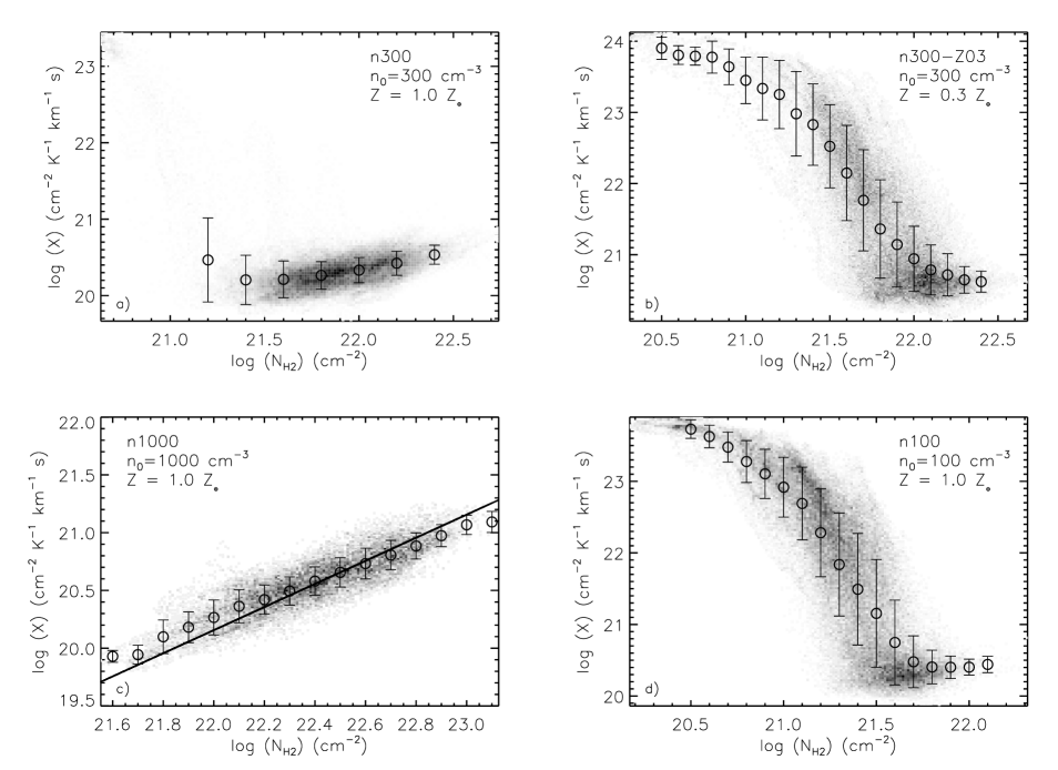
Figure 6: $X$ factor plotted against $N_{\rm H_{2}}$ for the 4 models shown in Figure 5. The (grey scale) color indicates the frequency of a given $N_{\rm H_{2}}$ and $X$ factor pair, where darker points indicate higher frequency. Black circles show average $X$ values in $N_{\rm H_{2}}$ bins, and the error bars indicate 1$\sigma$ deviations. The line in bottom left panel shows $X$ $\propto$ $N_{\rm H_{2}}$ relationship.

The models with lower metallicity and density (Figs. 6b and 6d) show a decreasing $X$ factor with increasing density (as can also be seen in Fig. 5). In this regime, an increase in the molecular density is associated with a greater increase in CO line intensity, resulting in a decrease in the $X$ factor. Such a trend is also present at the lowest densities of Model n300 (Fig. 6a).

Given that $W$ can have rather different distributions than $N_{\rm CO}$, it comes as no surprise that the $X$ factor does not neatly follow from $N_{\rm CO}$. For clouds with high CO abundances, such as models n300 and n1000, $N_{\rm CO}$ is well correlated with $N_{\rm H_{2}}$, resulting in a limited range in the distribution of the $X$ factor. We have seen that CO line saturation may not be discernible solely from the $X$ factor distributions, as evident from the similarity of the $X$ factor (normal) distributions of Model n300 (with saturation occurring only at the highest densities) and n1000 (which is close to fully saturated). The relationship between $X$ and $N_{\rm H_{2}}$ (Fig. 6), however, clearly demonstrates the saturation of the CO line. For the models with lower density or metallicity, where the $W$ - $N_{\rm H_{2}}$ correlation is rather complex, the $X$ factor can have a large distribution, and can even have multiple peaks in its PDF (such as Model n100, Fig 5d).

4 Discussion and Comparison to Observations

4.1 The Column Density Distributions: Can CO Observations Reveal Log-Normal PDFs?

Observed morphological characteristics, such as the density distribution, may be signatures of the internal dynamics of a cloud. Numerous simulations have shown that the (3D) volume density PDF is log-normal for non self-gravitating supersonic turbulent systems (see McKee & Ostriker, 2007, and references therein), which may be translated into log-normal PDFs of projected (2D) column density (Ostriker et al., 2001; Brunt et al., 2010b, a). Including gas self-gravity, which may counteract the dispersal due to turbulence so that some overdense regions may persist as bound objects, results in a PDF with a high density tail (Klessen, 2000). These signature high density tails have been found in column density PDFs obtained from observations of evolved clouds (Kainulainen et al., 2009). In general, however, directly correlating features of the PDF to physical processes in the simulation has proven to be rather difficult (Klessen, 2000; Federrath et al., 2008, 2010).

Understanding the relationship between CO and the underlying density distribution is essential if CO observations are employed as (molecular) mass tracers of MCs. Usually, density distributions are derived from ¹³CO intensities, since ¹³CO is optically thin (relative to ¹²CO). In our analysis of ¹²CO emission, we find that $W$ does not faithfully trace $N_{\rm CO}$ even in some low density regions. This is suggestive that ¹³CO intensities may also not be an ideal tracer of the underlying CO distribution. Though we analyze the density distribution traced by ¹²CO emission in this work, the suitability of ¹³CO as a column density tracer remains an open question that we plan on investigating in future work.

In practice, the shape of observed density PDFs strongly depends on the tracer observed. For instance, Goodman et al. (2009) found that dust observations of the Galactic MC Perseus show log-normal column density PDFs, and may provide reasonable estimates of the total mass. Gas (¹³CO) based measures result in PDFs with significantly different shapes, though a log-normal fit can loosely describe the distribution. In this section, we compare the PDFs of observed CO intensities with those of the intrinsic H₂ and CO column density (see Paper I for a discussion on the volume density PDFs).

We have found that the observed $W$ PDF can vary significantly from the column density PDFs, $N_{\rm CO}$ or $N_{\rm H_{2}}$, even though $N_{\rm H_{2}}$ (and $N_{\rm tot}$) for all models can be well described as log-normal distributions, as shown in Figure 2. Only models n300 and n1000 seemingly have $N_{\rm CO}$ and $W$ PDFs that can be well described as log-normals. For the PDFs of those models (Fig 2a,b,e,f), we have overplotted best fit log-normals, with functional form

$${\rm PDF}\propto e^{-(\log\,x-\log\,x_{0})/2\sigma^{2}},$$ (13)

where $x$ is $N_{\rm tot}$, $N_{\rm H_{2}}$, $N_{\rm CO}$, or $W$, $\sigma^{2}$ is the variance, and $x_{0}$ denotes the mean value. The distributions shown in Figure 2 show that the offsets in the log-normals do not coincide. Of course, this discrepancy is partly due to our choice of the axis ranges of $N_{\rm CO}$ and $W$. Thus, a comparison of $\sigma$, which is a measure of the width of the log-normal, is the parameter best suited for direct comparison between the PDFs.

For both models n300 and n1000, the $N_{\rm tot}$ and $N_{\rm H_{2}}$ PDFs have $\sigma=$ 0.3. For Model n300, $\sigma=$ 0.5 and 0.2 for the $N_{\rm CO}$ and $W$ PDFs, respectively. The best fits give $\sigma=$ 0.3 and 0.1 for the $N_{\rm CO}$ and $W$ PDFs, respectively, for Model n1000. As can be seen from the PDFs themselves, the best fits $N_{\rm CO}$ and $W$ log-normals are rather different for the two models. Such discrepancies are not surprising, given that the other models exhibit PDFs of $W$ and $N_{\rm CO}$ with vastly different forms.

That the $W$ and $N_{\rm CO}$ PDFs from Model n1000 are both log-normal, albeit with different characteristics, may be somewhat unexpected, given that this model is clearly affected by saturation (Figs. 1 and 6). With line saturation, one would expect the $W$ PDF to be asymmetric, with a prominent peak towards large intensities, and a sharp drop off beyond the peak - the “piled-up” effect discussed in Section 3.1. At any given extinction from Model n1000, even though much of the line emission from the highest density gas is saturated, there is a sufficiently large range of $W$ such that there is no sharp drop off in the $W$ PDF beyond the peak. This demonstrates that line saturation may be significant even when the PDF of the observed intensities does not show a sharp decrease. For such scenarios, it is only when inspecting $W$ with $N_{\rm tot}$ (Fig. 1) or $X$ with $N_{\rm H_{2}}$ (Fig. 6), for which independent estimates of $N_{\rm tot}$ or $N_{\rm H_{2}}$ would be required, that the presence of saturation can be inferred.

In general, we find that the $W$ PDFs are not log-normal, even though the underlying gas column densities are. One reason for the difference is that the $N_{\rm CO}$ PDFs themselves are not log-normal. Further, in most of the models, the $W$ PDF itself does not neatly follow that of $N_{\rm CO}$. Since CO traces the dense gas, $N_{\rm CO}$ is more intermittent than the underlying gas distribution. Due to the effects of saturation, this intermittency is not captured by $W$. In the two models with log-normal $W$ and $N_{\rm CO}$ PDFs, the variances between the distributions are nevertheless different. Taken together, we conclude that the distribution of observed CO intensities is not an accurate measure of the underlying distribution of molecular gas. This conclusion is affirmed by the observational analysis of Goodman et al. (2009), who found significant differences in the ¹³CO and dust-based distributions.

4.2 Globally Averaged X Factor

We have shown that, in general, the CO integrated intensity does not linearly trace $N_{\rm H_{2}}$, even within individual MCs, so that the $X$ factor is not constant. The intrinsic cloud properties, such as density, metallicity, and background UV radiation field, all influence how $W$ is related to $N_{\rm H_{2}}$. In the previous sections, our analysis has dealt with all positions in the 2D “observed” maps, which are idealized synthetic maps with high spatial resolution of $\sim$ 0.1 pc (the size of the grid zone in the MHD simulations). However, in practice the derived $X$ factor is likely to be an average over a range in extinction values, especially in observations of extragalactic clouds where the resolution may be comparable to the cloud size. In order for a more direct comparison with these types of integrated observations, we now shift our focus to the discussion of average quantities in the synthetic maps.

Figure 7 shows the mean $X$ factor in different $A_{V}$ bins for the four models shown in Figures 5-6, as well as Model n300-Z01. The emission-weighted mean $X$ and $A_{V}$ for each model is also shown (by the large symbols). A number of features of the averaged $X$ factor are similar to those already discussed: a decrease in $X$ with increasing extinction for models with low densities or metallicities, the opposite trend for Model n1000 (and to some extent Model n300) due to line saturation, and only a small variation in $X$ at high densities for Model n300. Qualitatively, the mean values of the $X$ factor binned with extinction resemble the extinction averaged quantities presented in Paper II (see their Fig. 8).

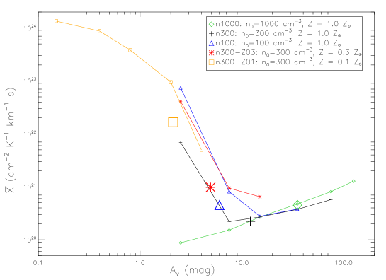
Figure 7: Mean $X$ factor in $A_{V}$ bins for 5 models. The $X$ factor is averaged in different $A_{V}$ bins. The value of $\overline{X}$ is plotted on the midpoint value of $A_{V}$ of each bin. Each model is identified by different colors and symbols (and labeled in the legend). The large symbols shows the global (emission weighted) mean $X$ factor and mean $A_{V}$ from each model.

One clear difference is that values of the $X$ factor averaged over a range in extinctions for a given model do not span as wide a range as when all positions are considered (compare, e.g. to Figs. 5-6). Only when comparing all the models at the low extinction $A_{V}$ $\buildrel<\over{\sim}$  5 does the large extent in the $X$ factor ($10^{20}<$ $X$ $<10^{24}$ cm^-2 K^-1 km^-1 s) become clear.

The striking feature of Figure 7 is the limited variation in the $X$ factor at large extinctions, both for a given model as well as between models. At extinctions  $\buildrel>\over{\sim}$ 7, $X$ falls in a narrow range $\sim 10^{20}$  $\buildrel<\over{\sim}$ $X$ $\buildrel<\over{\sim}$ $10^{21}$ cm^-2 K^-1 km^-1 s for all models. This range is similar to the $X$ factor values derived for the Galaxy (Solomon et al., 1987; Young & Scoville, 1991; Dame et al., 2001). The emission weighted mean $X$ and $A_{V}$ values (large symbols) also portray a near constant $X_{\rm Gal}$ value between the MCs, with the exception of the very low metallicity MC. Thus, only considering CO bright regions, corresponding to high extinctions, may not expose any real variation in the $N_{\rm H_{2}}$/$W$ ratio, as discussed in Paper II.

Observations of the Small Magellanic Cloud (SMC), which has lower than Galactic metallicity, has resulted in high $X$ factor estimates (Israel, 1997; Leroy et al., 2009, and references therein). Averaged over a whole cloud in the SMC, Leroy et al. (2009) found that the $X$ factor varies by  $\buildrel>\over{\sim}$ 1 order of magnitude, whereas the $X$ factor computed at the CO peaks is similar to the Galactic value. Our analysis of CO emission from models with lower metallicity, especially Model n300-Z03, which has a metallicity similar to that of SMC (Vermeij & van der Hulst, 2002), quantitatively reproduces the estimated $X$ factor, both the larger value due to diffuse gas and the lower Galactic value found in the densest regions.

4.3 $X$ Factor in Dense and Diffuse Gas

In our discussion of the Galactic $X$ factor, we have focused on observations of molecular clouds (e.g. Young & Scoville, 1991; Solomon et al., 1987). However, CO has also been detected in the diffuse ISM (e.g. Polk et al., 1988; Burgh et al., 2007), and the $X$ factor for these diffuse lines of sight is found to be consistent with the standard galactic value of $X_{\rm Gal}$ (few $\times 10^{20}$ cm^-2 K^-1 km^-1 s, Liszt et al., 2010). Though we consider models of individual (or large volumes within) MCs, we investigate whether regions with different densities are comparable with the observations of different phases of the ISM, focusing on the recent discussion on the uniformity of the $X$ factor in Liszt et al. (2010), hereafter LPL10.

LPL10 find that diffuse gas, with molecular column densities $N_{\rm H_{2}}$ $\sim$ 10²⁰–10²¹ cm^-2, and dense Galactic clouds, characterized by $N_{\rm H_{2}}$ $\sim$ 10²³ cm^-2, are always found to have $X$ factor values that are $\sim$$X_{\rm Gal}$. Since the $X$ factor can be written as

$$X=\left(\frac{N_{\rm CO}}{W}\right)\left(\frac{N_{\rm H_{2}}}{N_{\rm CO}}\right)=\frac{N_{\rm CO}}{W}\frac{1}{f_{\rm CO}},$$ (14)

LPL10 attribute the constancy of the $X$ factor to the increase in the specific brightness, $W/N_{\rm CO}$, in low density, warm gas, by a factor comparable to the decrease in $f_{\rm CO}=N_{\rm CO}/N_{\rm H_{2}}$. For diffuse gas, LPL10 use an estimate of $f_{\rm CO}\approx 3\times 10^{-6}$, based on Burgh et al. (2007), while for dense gas, they adopt $f_{\rm CO}\approx 10^{-4}$. These values correspond to $W/N_{\rm CO}\approx 10^{-15}$ and $3\times 10^{-17}$ K km s^-1 cm², in diffuse and dense gas, respectively, for a constant $X$ factor $=3\times 10^{20}$ cm^-2 K^-1 km^-1 s.

As discussed, we have found that the Milky Way model n300 does indeed result in $X$$\approx$$X_{\rm Gal}$ in most lines of sight. In this model, there is only a very small fraction of the simulated volume with the lowest H₂ column densities $N_{\rm H_{2}}$ $\buildrel<\over{\sim}$ $10^{21}$ cm^-2 (see Fig. 5a). Thus, for comparison with LPL10 we will use model n300-Z03, which has many lines of sight with both dense ($N_{\rm H_{2}}$$\sim 10^{22}$) and diffuse gas ($N_{\rm H_{2}}$$\sim 5\times 10^{20}$). Maps of the various relevant quantities for this model are presented in Figure 4. Though this model has lower metallicity ($Z$ = 0.3Z_⊙) than the observations of LPL ($Z$=Z_⊙), a comparison of the observations with Model n100, (or the high density gas in Model n300) bear similar results as those provided by Model n300-Z03.

We identify dense gas as regions with log($W$) $>$ 1.5, marked by dashed contours in Fig. 4, and compute $W/N_{\rm CO}\in 4\times 10^{-17}-8\times 10^{-16}$ K km s^-1 cm². The lower and upper limits have corresponding $f_{\rm CO}$ values of $5\times 10^{-5}$ and $5\times 10^{-6}$, respectively. The resulting value of the $X$ factor is $\sim 1-6\times 10^{20}$ cm^-2 K^-1 km^-1 s. These values of $W/N_{\rm CO}$, $f_{\rm CO}$, and $X$, reasonably reproduce the values determined by LPL10 for dense clouds, with an $X$ factor which only differs by at most a factor of 3.

The low density regions of Model n300-Z03, marked roughly by the log($W$) $<$ -1 contour in Fig. 4, have $W/N_{\rm CO}\sim 10^{-15}$ K km s^-1 cm², and $f_{\rm CO}\sim 6\times 10^{-10}$, resulting in an $X$ factor $\sim 10^{24}$ cm^-2 K^-1 km^-1 s. This $X$ factor differs from the LPL10 estimated value from observations of diffuse gas by up to 4 orders of magnitude. The discrepancy can be almost fully attributed to the difference in $f_{\rm CO}$ between our models and the LPL10 observations; the values of $W/N_{\rm CO}$ of our models and that determined by the LPL10 analysis only differ by a factor of $\sim$ 2 - 10. Table 2 summarizes the comparison of $W/N_{\rm CO}$, $f_{\rm CO}$, and $X$ between Model n300-Z03 and LPL10 in the dense and diffuse gas.

Table 2: Comparison of Model n300-Z03 and Liszt et al. (2010) Observations

Gas Phase	$N_{\rm H_{2}}$ (cm-2)	$f_{\rm CO}$	$W/N_{\rm CO}$	$X$ (cm-2 K-1 km-1 s)
Observed Dense Gas (LPL10)	$\sim 10^{23}$	$\sim 10^{-4}$	$\sim 3\times 10^{-17}$	$\sim 3\times 10^{20}$
Dense Gas in Simulation (n300-Z03)	$\sim 2-4\times 10^{22}$	$\sim 0.5-5\times 10^{-5}$	$\sim 0.4-8\times 10^{-16}$	$\sim 1-6\times 10^{20}$
Observed Diffuse Gas (LPL10)	$\sim 10^{20}-10^{21}$	$\sim 3\times 10^{-6}$	$\sim 10^{-15}$	$\sim 3\times 10^{20}$
Low Density Gas in Simulation (n300-Z03)	$\sim 2-7\times 10^{20}$	$\sim 6\times 10^{-10}$	$\sim 10^{-15}$	$\sim 10^{24}$

The comparison of the characteristics of the dense regions has quantitatively affirmed some level of accuracy of the chemical (and MHD) modeling, as well as the radiative transfer calculations. Additionally, we can draw some insights from the discrepancy we find in the characteristics of the diffuse regions: the larger difference in $f_{\rm CO}$ in our models compared to the LPL10 observations of tenuous gas, rather than $W/N_{\rm CO}$, indicates that the chemical processes at work in the low density regions within our molecular clouds are very different from the chemistry of diffuse Milky Way gas. That $f_{\rm CO}$ is significantly lower in the low density regions of the model suggests that either CO forms at a greater rate in the diffuse ISM (relative to the rate in the model), or that CO is efficiently transported into the diffuse ISM (and has sufficient shielding against photodissociation). The physical processes at work in our models, turbulence, magnetic fields, or simply even the uniform metallicities (or initial densities), may be significantly different in the tenuous ISM. In particular, non-thermal chemistry in C-shocks or turbulent vortices may play an important role in the chemistry of the diffuse gas (see e.g. Federman et al., 1996; Sheffer et al., 2008; Godard et al., 2009). Alternatively, large scale galactic processes not considered in our model may be required to accurately model the chemistry in diffuse molecular gas, such as galactic rotation, the gravitational field due to the disk, and/or large scale magnetic fields. We hope to pursue studies involving such large scale dynamics and chemistry in the future.

4.4 Future Work: $X$ factors as Mass Estimators for CO Bright Cores?

In observational investigations where the $X$ factor is derived solely from CO observations, the CO linewidths are used to derive masses through the virial theorem. If the bulk of the gas is in molecular form, then $W$ is employed along with the CO linewidth derived $N_{\rm H_{2}}$ to estimate the $X$ factor via Equation 1. The key assumption here is that the observed clouds are in virial equilibrium (e.g. Young & Scoville, 1991; Solomon et al., 1987), which is the interpretation of the observed power-law linewidth $\sigma_{v}$ size $R$ relationship $\sigma_{v}\propto R^{0.5}$ (e.g. Larson, 1981; Solomon et al., 1987). Measurements of the molecular mass through independent observations, such as dust-based emission or extinction, can also provide estimates of $N_{\rm H_{2}}$. These can be combined with CO observations to calculate the $X$ factor. As discussed in Section 1, a discrepancy in the derived $X$ factor based on virialized clouds or based on independent H₂ mass estimates is found in low metallicity systems, such as the SMC (Bolatto et al., 2008; Rubio et al., 2004; Israel, 1997; Leroy et al., 2007; Leroy et al., 2009).

The velocity dispersions in our models follow the observed $\sigma_{v}\propto R^{0.5}$ relationship (Shetty et al. In preparation), as found in numerous similar turbulent cloud models (e.g. Klessen, 2000; Ostriker et al., 2001; Federrath et al., 2010). We have calculated the $X$ factors in model MCs assuming independent knowledge of $N_{\rm H_{2}}$, so no assumption of a linewidth-size scaling, or of virialized clouds (or cores), is necessary. In our analysis of total column densities and integrated intensities, we find that $X$ factor is primarily controlled by the CO abundance, and thus ultimately by cloud properties most responsible for CO formation: the metallicity, density, or background UV radiation field. This variation in the $X$ factor is most drastic - upto several orders of magnitude - in models with metallicities, densities, or UV radiation fields different from the Milky Way. These results are in agreement with models showing an increased $X$ factor for low metallicity systems (Maloney & Black, 1988; Israel, 1997).

The discrepancy between $X$ factor estimates based on virialized systems, and those based on independent $N_{\rm H_{2}}$ measures can be explained by the selective photodissociation of CO in low density regions. The CO bright objects thus only trace highest density gas, which is surrounded by lower density molecular material, with little or no CO emission (Maloney & Black, 1988; Bolatto et al., 2008; Grenier et al., 2005; Wolfire et al., 2010, Paper II, Molina et al. in prep.). In low metallicity or low density systems, we only find the $X$ factor to be constant at the very highest densities (Figs. 6b & 6d), though the vast majority of observed points clearly show a gradient in the $X$ factor with density. For the high density Model n1000 (Fig 6c), the $X$ factor increases with increasing density due to CO line saturation (Fig. 1c), though the range of $X$ is only  $\buildrel<\over{\sim}$  2 orders of magnitude.

The idea that CO observations accurately provide mass estimates, with $X$$\approx$$X_{\rm Gal}$, of virialized clouds needs to be affirmed quantitatively. Previous efforts to address this issue have usually involved static models. Kutner & Leung (1985) constructed clouds models with microturbulent velocities consistent with the observed linewidth-size relationship. They found that the $X$ factor still strongly depends on the temperature, as well as the density and CO abundance. Using photodissociation region models, Wolfire et al. (1993) found that microturbulence cannot reproduce the observed CO line profiles. The CO intensity, and hence the $X$ factor, is sensitive to other parameters responsible for CO formation. With the radiative transfer calculations performed on the 3D MHD simulations including chemistry discussed here, we can further investigate how various turbulent velocity fields influence CO emission, as well as the cloud characteristics that affect the $X$ factor in a range of environments.

Such an analysis would address the following issues: How well do CO peaks trace coherent objects in spectral (PPV) cubes? Identifying coherent objects from spectral cubes has proved to be quite challenging, as a consequence of line-of-sight projection (Adler & Roberts, 1992; Pichardo et al., 2000). How well do CO linewidths encode information on the dynamics of the cloud? Projection effects may also skew the linewidth - size power law scalings (Ballesteros-Paredes et al., 1999; Ballesteros-Paredes & Mac Low, 2002; Shetty et al., 2010). If a CO bright core can be accurately identified, is the observed linewidth representative of the intrinsic velocity dispersion? To what extent does turbulence affect the CO emission, and thus the $X$ factor? These issues will all be visited and discussed in a forthcoming paper.

5 Summary

We have performed radiative transfer calculations to investigate the nature of ¹²CO (J=1-0) emission from simulations of molecular clouds (MCs). The MCs are modeled through hydrodynamic simulations of a turbulent, magnetized, non self-gravitating gaseous medium, along with a treatment of chemistry to track the formation of H₂ and CO (Paper I and Paper II). As part of the radiative transfer calculations, we use the Sobolev (LVG) method to solve for the CO level populations. We analyze the probability distribution functions, and $X$ factor properties, using the velocity integrated CO intensities $W$, along with the column density of CO and H₂, $N_{\rm CO}$ and $N_{\rm H_{2}}$, respectively. Our main findings are:

1) In all models, $W$ increases with increasing total hydrogen column density $N_{\rm tot}$ (or extinction $A_{V}$). However, for the Milky Way and high density models (n300 and n1000), which have the highest CO abundances, we find a threshold in $W$$\approx$65 K km s^-1 at high extinction due to saturation of the CO line.

2) All models have log-normal $N_{\rm tot}$ and $N_{\rm H_{2}}$ distributions. In general, however, the $W$ and $N_{\rm CO}$ PDFs are not log-normal. Further, since CO is optically thick, the $W$ PDFs do not have similar shapes to the corresponding $N_{\rm CO}$ PDFs.

3) In some models for which the CO line is saturated, the peak in $N_{\rm CO}$ is offset towards higher densities than the peak in $W$, though the two PDFs seem to be correlated at low densities. However, such a “piled-up” $W$ PDF does not necessarily arise in clouds with saturated CO emission, especially those with a limited range in densities (as for the high density model n1000, Figs. 1-2). Independent measurements of $N_{\rm tot}$ or $N_{\rm H_{2}}$, along with $W$, are needed to unambiguously identify saturation.

4) The $X$ factor is not constant within individual molecular clouds, and in models with low CO fractions, can vary by up to 4 orders of magnitude. The low density regions have the highest $X$ factor, in agreement with previous modeling efforts.

5) In most simulations, the averaged $X$ factor is found to be similar to $X_{\rm Gal}$ ($\sim 2\times 10^{20}$ cm^-2 K^-1 km^-1 s), masking the variation of $X$ with density within clouds. In clouds with low CO abundances relative to the Galaxy (such as the model MC in a dwarf galaxy or the LMC/SMC), the densest regions have $X$ $\sim$ $X_{\rm Gal}$.

6) Emission weighted averaged $X$ factors from all models provide values $\approx$$X_{\rm Gal}$  with the exception of the very low metallicity MC (n300-Z01). Similarly, at extinctions $A_{V}$  $\buildrel>\over{\sim}$ 7, the $X$ factor for always falls in a narrow range $\sim 10^{20}$  $\buildrel<\over{\sim}$ $X$ $\buildrel<\over{\sim}$ $10^{21}$ cm^-2 K^-1 km^-1 s. As discussed in Paper II, observations targeting CO bright regions may be unable to detect real variations in the $X$ factor.

7) In the low density gas within the MC models, the CO fraction $f_{CO}$ is found to be $\sim$ three orders of magnitude lower than $f_{CO}$ measured by Burgh et al. (2007) in diffuse gas. That $N_{\rm H_{2}}$ and $W$/$N_{\rm CO}$ are comparable between the model and the observations suggest that the dynamics and chemical evolution of diffuse gas in our molecular cloud model are rather different from that in the large scale diffuse gas of the Galaxy.

8) We do not assume that clouds or cores are in virial equilibrium, and the $X$ factor variations we find are in general agreement with observational analyses employing independent measures of total molecular column densities. In a follow up investigation, we will use the spectral information of our models to assess the $X$ factor when virial equilibrium is assumed; we will then be able to address the $X$ factor discrepancy found in observational works when assuming virialized CO clouds or when using independent molecular mass estimates.

References

- Adler & Roberts (1992) Adler D. S., Roberts Jr. W. W., 1992, ApJ, 384, 95
- Ballesteros-Paredes et al. (2007) Ballesteros-Paredes J., Klessen R. S., Mac Low M., Vazquez-Semadeni E., 2007, Protostars and Planets V, pp 63–80
- Ballesteros-Paredes & Mac Low (2002) Ballesteros-Paredes J., Mac Low M.-M., 2002, ApJ, 570, 734
- Ballesteros-Paredes et al. (1999) Ballesteros-Paredes J., Vázquez-Semadeni E., Scalo J., 1999, ApJ, 515, 286
- Bohlin et al. (1978) Bohlin R. C., Savage B. D., Drake J. F., 1978, ApJ, 224, 132
- Bolatto et al. (2008) Bolatto A. D., Leroy A. K., Rosolowsky E., Walter F., Blitz L., 2008, ApJ, 686, 948
- Brunt et al. (2010a) Brunt C. M., Federrath C., Price D. J., 2010a, MNRAS, 405, L56
- Brunt et al. (2010b) Brunt C. M., Federrath C., Price D. J., 2010b, MNRAS, 403, 1507
- Burgh et al. (2007) Burgh E. B., France K., McCandliss S. R., 2007, ApJ, 658, 446
- Castor (1970) Castor J. I., 1970, MNRAS, 149, 111
- Dame et al. (2001) Dame T. M., Hartmann D., Thaddeus P., 2001, ApJ, 547, 792
- Dickman (1978) Dickman R. L., 1978, ApJS, 37, 407
- Elitzur (1992) Elitzur M., ed. 1992, Astronomical masers Vol. 170 of Astrophysics and Space Science Library
- Federman et al. (1996) Federman S. R., Rawlings J. M. C., Taylor S. D., Williams D. A., 1996, MNRAS, 279, L41
- Federrath et al. (2008) Federrath C., Klessen R. S., Schmidt W., 2008, ApJL, 688, L79
- Federrath et al. (2010) Federrath C., Roman-Duval J., Klessen R. S., Schmidt W., Mac Low M., 2010, A&A, 512, A81+
- Ferrière (2001) Ferrière K. M., 2001, Reviews of Modern Physics, 73, 1031
- Glover et al. (2010) Glover S. C. O., Federrath C., Mac Low M., Klessen R. S., 2010, MNRAS, 404, 2 (Paper I)
- Glover & Mac Low (2007a) Glover S. C. O., Mac Low M., 2007a, ApJS, 169, 239
- Glover & Mac Low (2007b) Glover S. C. O., Mac Low M., 2007b, ApJ, 659, 1317
- Glover & Mac Low (2010) Glover S. C. O., Mac Low M., 2010, ArXiv e-prints 1003.1340 (Paper II)
- Godard et al. (2009) Godard B., Falgarone E., Pineau Des Forêts G., 2009, A&A, 495, 847
- Goodman et al. (2009) Goodman A. A., Pineda J. E., Schnee S. L., 2009, ApJ, 692, 91
- Grenier et al. (2005) Grenier I. A., Casandjian J., Terrier R., 2005, Science, 307, 1292
- Heithausen et al. (1993) Heithausen A., Stacy J. G., de Vries H. W., Mebold U., Thaddeus P., 1993, A&A, 268, 265
- Israel (1997) Israel F. P., 1997, A&A, 328, 471
- Israel et al. (1986) Israel F. P., de Graauw T., van de Stadt H., de Vries C. P., 1986, ApJ, 303, 186
- Kainulainen et al. (2009) Kainulainen J., Beuther H., Henning T., Plume R., 2009, A&A, 508, L35
- Klessen (2000) Klessen R. S., 2000, ApJ, 535, 869
- Kutner & Leung (1985) Kutner M. L., Leung C. M., 1985, ApJ, 291, 188
- Larson (1981) Larson R. B., 1981, MNRAS, 194, 809
- Leroy et al. (2007) Leroy A., Bolatto A., Stanimirovic S., Mizuno N., Israel F., Bot C., 2007, ApJ, 658, 1027
- Leroy et al. (2009) Leroy A. K., Bolatto A., Bot C., Engelbracht C. W., Gordon K., Israel F. P., Rubio M., Sandstrom K., Stanimirović S., 2009, ApJ, 702, 352
- Li et al. (2003) Li Y., Klessen R. S., Mac Low M., 2003, ApJ, 592, 975
- Liszt et al. (2010) Liszt H. S., Pety J., Lucas R., 2010, A&A, 518, A45 (LPL10)
- Lombardi et al. (2006) Lombardi M., Alves J., Lada C. J., 2006, A&A, 454, 781
- Mac Low & Klessen (2004) Mac Low M., Klessen R. S., 2004, Reviews of Modern Physics, 76, 125
- Maloney & Black (1988) Maloney P., Black J. H., 1988, ApJ, 325, 389
- McKee & Ostriker (2007) McKee C. F., Ostriker E. C., 2007, ARA&A, 45, 565
- Mihalas (1978) Mihalas D., 1978, Stellar atmospheres /2nd edition/
- Norman (2000) Norman M. L., 2000, in S. J. Arthur, N. S. Brickhouse, & J. Franco ed., Revista Mexicana de Astronomia y Astrofisica Conference Series Vol. 9 of Revista Mexicana de Astronomia y Astrofisica Conference Series, Introducing ZEUS-MP: A 3D, Parallel, Multiphysics Code for Astrophysical Fluid Dynamics. pp 66–71
- Ossenkopf (1997) Ossenkopf V., 1997, New Astronomy, 2, 365
- Ostriker et al. (2001) Ostriker E. C., Stone J. M., Gammie C. F., 2001, ApJ, 546, 980
- Pichardo et al. (2000) Pichardo B., Vázquez-Semadeni E., Gazol A., Passot T., Ballesteros-Paredes J., 2000, ApJ, 532, 353
- Pineda et al. (2008) Pineda J. E., Caselli P., Goodman A. A., 2008, ApJ, 679, 481
- Polk et al. (1988) Polk K. S., Knapp G. R., Stark A. A., Wilson R. W., 1988, ApJ, 332, 432
- Rubio et al. (2004) Rubio M., Boulanger F., Rantakyro F., Contursi A., 2004, A&A, 425, L1
- Schöier et al. (2005) Schöier F. L., van der Tak F. F. S., van Dishoeck E. F., Black J. H., 2005, A&A, 432, 369
- Sheffer et al. (2008) Sheffer Y., Rogers M., Federman S. R., Abel N. P., Gredel R., Lambert D. L., Shaw G., 2008, ApJ, 687, 1075
- Shetty et al. (2010) Shetty R., Collins D. C., Kauffmann J., Goodman A. A., Rosolowsky E. W., Norman M. L., 2010, ApJ, 712, 1049
- Sobolev (1957) Sobolev V. V., 1957, Soviet Astronomy, 1, 678
- Solomon et al. (1987) Solomon P. M., Rivolo A. R., Barrett J., Yahil A., 1987, ApJ, 319, 730
- Stone & Norman (1992a) Stone J. M., Norman M. L., 1992a, ApJS, 80, 753
- Stone & Norman (1992b) Stone J. M., Norman M. L., 1992b, ApJS, 80, 791
- van der Tak et al. (2007) van der Tak F. F. S., Black J. H., Schöier F. L., Jansen D. J., van Dishoeck E. F., 2007, A&A, 468, 627
- van Dishoeck & Black (1988) van Dishoeck E. F., Black J. H., 1988, ApJ, 334, 771
- Vazquez-Semadeni (1994) Vazquez-Semadeni E., 1994, ApJ, 423, 681
- Vermeij & van der Hulst (2002) Vermeij R., van der Hulst J. M., 2002, A&A, 391, 1081
- Wolfire et al. (2010) Wolfire M. G., Hollenbach D., McKee C. F., 2010, ApJ, 716, 1191
- Wolfire et al. (1993) Wolfire M. G., Hollenbach D., Tielens A. G. G. M., 1993, ApJ, 402, 195
- Yang et al. (2010) Yang B., Stancil P. C., Balakrishnan N., Forrey R. C., 2010, ApJ, 718, 1062
- Young & Scoville (1991) Young J. S., Scoville N. Z., 1991, ARA&A, 29, 581