Comparison of Spearman’s rho and Kendall’s tau in Normal and Contaminated Normal Models

Abstract

This paper analyzes the performances of the Spearman’s rho (SR) and Kendall’s tau (KT) with respect to samples drawn from bivariate normal and bivariate contaminated normal populations. The exact analytical formulae of the variance of SR and the covariance between SR and KT are obtained based on the Childs’s reduction formula for the quadrivariate normal positive orthant probabilities. Close form expressions with respect to the expectations of SR and KT are established under the bivariate contaminated normal models. The bias, mean square error (MSE) and asymptotic relative efficiency (ARE) of the three estimators based on SR and KT to the Pearson’s product moment correlation coefficient (PPMCC) are investigated in both the normal and contaminated normal models. Theoretical and simulation results suggest that, contrary to the opinion of equivalence between SR and KT in some literature, the behaviors of SR and KT are strikingly different in the aspects of bias effect, variance, mean square error, and asymptotic relative efficiency. The new findings revealed in this work provide not only deeper insights into the two most widely used rank based correlation coefficients, but also a guidance for choosing which one to use under the circumstances where the PPMCC fails to apply.

I Introduction

Correlation analysis is among the core research paradigms in nearly all branches of scientific and engineering fields, not to mention the area of information theory [1, 2, 3, 4, 5, 6, 7, 8, 9, 10]. Being interpreted as the strength of statistical relationship between two random variables [11], correlation should be large and positive if there is a high probability that large (small) values of one variable occur in conjunction with large (small) values of another; and it should be large and negative if the direction is reversed [12]. A number of methods have been proposed and applied in the literature to assess the correlation between two random variables. Among these methods the Pearson’s product moment correlation coefficient (PPMCC) [13, 14], Spearman’s rho (SR) [15] and Kendall’s tau (KT) [15] are perhaps the most widely used [16].

The properties of PPMCC in bivariate normal samples (binormal model) is well known thanks to the creative work of Fisher [13]. It follows that, in the normal cases, 1) PPMCC is an asymptotic unbiased estimator of the population correlation $\rho$, and 2) the variance of PPMCC approaches the Cramer-Rao lower bound (CRLB) with increase of the sample size [11]. Due to its optimality, PPMCC has and will continue to play the dominant role when quantifying the intensity of correlation between bivariate random variables in the literature. However, sometimes the PPMCC might not be applicable when the following scenarios happen:

1. The data is incomplete, that is, only ordinal information (e.g. ranks) is available. This situation is not uncommon in the area of social sciences, such as psychology and education [15];

2. The underlying data is complete (cardinal) and follows a bivariate normal distribution, but is attenuated more or less by some monotone nonlinearity in the transfer characteristics of sensors [17];

3. The data is complete and the majority follows a bivariate normal distribution, but there exists a tiny fraction of outliers (impulsive noise) [18, 19, 20].

Under these circumstances, it would be more suitable to employ the two most popular nonparametric coefficients, SR and KT, which are 1) dependant only on ranks, 2) invariant under increasing monotone transformations [15], and 3) robust against impulsive noise [21]. Now we are at a stage to ask the question: which one, SR or KT, should we use in Scenarios 1) to 3) where the familiar PPMCC is inapplicable? Unfortunately, however, despite the rich history of SR and KT, the answers to this question are still inconsistent in the literature. Some researchers, such as Fieller et al[22], preferred KT to SR based on empirical evidences; while others, such as Gilpin [23], asserted that SR and KT are equivalent.

Aiming at resolving such inconsistency, in this work we investigate systematically the properties of SR and KT under the binormal model [24, 25, 26]. Moreover, to deal with Scenario 3) mentioned above, we also investigate their properties under the contaminated binormal model [18, 19, 20]. Our theoretical contribution is multifold. Firstly, we find a computationally more tractable formula of the variance of SR. Based on this formula, we provide the densely tabulated Table I with high precision (ten decimal places). This table overcomes the shortcomings of the existing power-series-based approximations that are tedious to use and of rather limited precision (up to five decimal places and for $\rho\leq 0.8$ only) [27, 28, 22, 29]. Secondly, we derive the exact analytical expression of the covariance between SR and KT. With this new analytical result, we uncover a minor error in the literature [28, 15]. Thirdly, we obtain the asymptotic expressions of the variances and hence the asymptotic relative efficiencies (AREs) concerning the three estimators of the population correlation $\rho$ based on SR and KT. Finally, we find the asymptotic expressions with respect to the expectations of SR and KT under the contaminated normal model.

The rest part of this paper is structured as follows. Section II gives some basic definitions and summarizes the general properties of PPMCC, SR and KT. In Section III, we lay the foundation of the theoretical framework in this study by outlining some critical results in the binormal model. Section IV establishes, in the bivariate normal model, 1) the exact expression of the variance of SR, 2) two exact expressions concerning the covariance between SR and KT, and, 3) in the contaminated normal model, the closed form formulae associated with the expectations of SR and KT, respectively. In Section V we focus on the performances of the three estimators of $\rho$ constructed from SR and KT. Section VI verifies the analytical results with Monte Carlo simulations. Finally, in Section VII we provide our answers to the above raised question concerning the choice of Spearman’s rho and Kendall’s tau in practice when PPMCC fails to apply.

II Basic Definitions and General Properties

II-A Definitions

Let $\{(X_{i},Y_{i})\}_{i=1}^{n}$ denote $n$ independent and identically distributed (i.i.d.) data pairs drawn from a bivariate population with continuous joint distribution. Suppose that $X_{j}$ is at the $k$th position in the sorted sequence $X_{(1)}<\cdots<X_{(n)}$. The number $k$ is termed the rank of $X_{j}$ and is denoted by $P_{j}$. Similarly we can get the rank of $Y_{j}$ which is denoted by $Q_{j}$ [15]. Let $\bar{X}$ and $\bar{Y}$ be the arithmetic mean values of $X_{i}$ and $Y_{i}$, respectively. Let $\mathrm{sgn}(\blacktriangle)$ stand for the sign of the argument $\blacktriangle$. The three well known classical correlation coefficient, PPMCC ($r_{P}$), SR ($r_{S}$), and KT ($r_{K}$), are then defined as follows [12]:

$$r_{P}(X,Y) \triangleq\frac{\sum\limits_{i=1}^{n}\left(X_{i}-\bar{X}\right)\left(Y_{i}-\bar{Y}\right)}{\left[\sum\limits_{i=1}^{n}\left(X_{i}-\bar{X}\right)^{2}\sum\limits_{i=1}^{n}\left(Y_{i}-\bar{Y}\right)^{2}\right]^{\frac{1}{2}}}$$ (1)

$$r_{S}(X,Y) \triangleq 1-\frac{6\sum\limits_{i=1}^{n}(P_{i}-Q_{i})^{2}}{n(n^{2}-1)}$$ (2)

$$r_{K}(X,Y) \triangleq\frac{\underset{i\neq j=1}{\sum\limits^{n}\sum\limits^{n}}\,\,\mathrm{sgn}\left(X_{i}-X_{j}\right)\mathrm{sgn}\left(Y_{i}-Y_{j}\right)}{n(n-1)}.$$ (3)

To ease the following discussion, we will employ the symbol $r_{\lambda}(X,Y)$, $\lambda\in\{P,S,K\}$ as a compact notation for the three coefficients. For brevity, the arguments of $r_{\lambda}(X,Y)$ will be dropped in the sequel unless ambiguity occurs.

II-B General Properties

It follows that coefficients $r_{\lambda}$, $\lambda\in\{P,S,K\}$ possess the following general properties:

1. $r_{\lambda}(X,Y)\in[-1,1]$ for all $(X,Y)$ (standardization);

2. $r_{\lambda}(X,Y)=r_{\lambda}(Y,X)$ (symmetry);

3. $r_{\lambda}=\pm 1$ if $Y$ is a positive (negative) linear transformation of $X$ (shift and scale invariance);

4. $r_{S}{=}r_{K}{=}\pm 1$ if $Y$ is a monotone increasing (decreasing) function of $X$ (monotone invariance);

5. The expectations of $r_{\lambda}$ equal zero if $X$ and $Y$ are independent (independence);

6. $r_{\lambda}(+,+)=-r_{\lambda}(-,+)=-r_{\lambda}(+,-)=r_{\lambda}(-,-)$;

7. $r_{\lambda}$ converges to normal distribution when the sample size $n$ is large.

Note that the first six properties are discussed in [12] and [16], and the last property follows from the asymptotic theory of $U$-statistics established by Hoeffding [30].

II-C Relationships Among PPMCC, SR and KT

From their expressions (1)–(3), it appears that the three coefficients PPMCC, SR and KT are quite different. However, as demonstrated below, these three coefficients are closely related with each other.

II-C1 Daniel’s Generalized Correlation Coefficient

Consider the $n$ data pairs $(X_{i},Y_{i})$, $i=1,\ldots,n$, at hand. To each pair of $X$’s, ($X_{i},X_{j}$), we can allot a score $a_{ij}$ such that $a_{ij}=-a_{ji}$ and $a_{ii}=0$. In a similar manner, we can also allot a sore $b_{ij}$ to the ordered pair of $Y$’s, ($Y_{i},Y_{j}$). The Daniel’s generalized coefficient $\Gamma$ is then defined by [31]

$$\Gamma\triangleq\frac{\sum\limits_{i=1}^{n}\sum\limits_{j=1}^{n}a_{ij}b_{ij}}{\left(\sum\limits_{i=1}^{n}\sum\limits_{j=1}^{n}a_{ij}^{2}\sum\limits_{i=1}^{n}\sum\limits_{j=1}^{n}b_{ij}^{2}\right)^{\frac{1}{2}}}.$$ (4)

This general setup covers PPMCC, SR and KT as special cases with respect to different systems of scores [31]:

• Replacing $a_{ij}$ by $X_{j}{-}X_{i}$ and $b_{ij}$ by $Y_{j}{-}Y_{i}$ in (4) gives the PPMCC $r_{P}$ defined in (1);

• Replacing $a_{ij}$ by $P_{j}{-}P_{i}$ and $b_{ij}$ by $Q_{j}{-}Q_{i}$ in (4) gives the SR $r_{S}$ defined in (2);

• Replacing $a_{ij}$ by $\mathrm{sgn}(X_{j}{-}X_{i})$ and $b_{ij}$ by $\mathrm{sgn}(Y_{j}{-}Y_{i})$ in (4) gives the KT $r_{K}$ defined in (3).

II-C2 Inequalities between SR and KT

It is possible to state certain inequalities connecting the values of SR and KT based on a given set of $n$ observations. The first one, ascribed to Daniel [32], is

$$-1\leq\frac{3(n+2)}{n-2}r_{K}-\frac{2(n+1)}{n-2}r_{S}\leq 1$$ (5)

which, for large $n$, becomes

$$-1\leq 3r_{K}-2r_{S}\leq 1.$$

The second one, due to Durbin and Stuat [33], states that

$$r_{S}\leq 1-\frac{1-r_{K}}{2(n+1)}\left[(n-1)(1-r_{K})+4\right].$$ (6)

Combing (5) and (6) and letting $n\to\infty$ yield the bounds of SR, in terms of KT, as

$$\frac{3}{2}r_{K}-\frac{1}{2} \leq r_{S}\leq\frac{1}{2}+r_{K}-\frac{1}{2}r_{K}^{2},\quad r_{K}\geq 0$$

$$\frac{3}{2}r_{K}+\frac{1}{2} \geq r_{S}\geq\frac{1}{2}r_{K}^{2}+r_{K}-\frac{1}{2},\quad r_{K}\leq 0.$$

II-C3 Relationship of SR to Other Coefficients

Besides the PPMCC and KT, SR is also closely related to other correlation coefficients, e.g., the order statistics correlation coefficient (OSCC) [34, 35, 36] and the Gini correlation (GC) [37]. In fact, SR can be reduced from the OSCC and GC by replacing the variates with corresponding ranks [38].

III Auxiliary Results in Normal Cases

In this section we provide some prerequisites concerning the orthant probabilities of normal distributions. These probabilities, contained in Lemma 1, are critical for the development of Theorem 1 and Theorem 2 later on. Moreover, some well known results about the expectation and variance of PPMCC, SR and KT are collected in Lemma 2 for ease of exposition. For convenience, we use symbols $\mathbb{E}(\blacktriangle)$, $\mathbb{V}(\blacktriangle)$, $\mathbb{C}(\blacktriangle,\blacklozenge)$, and $\mathrm{corr}(\blacktriangle,\blacklozenge)$ in the sequel to denote the mean, variance, covariance, and correlation of (between) random variables, respectively. Symbols of big oh and little oh are utilized to compare the magnitudes of two functions $u(\blacktriangle)$ and $v(\blacktriangle)$ as the argument $\blacktriangle$ tends to a limit $L$ (might be infinite). The notation $u(\blacktriangle)=O(v(\blacktriangle))$, $\blacktriangle{\to}L$, denotes that $|u(\blacktriangle)/v(\blacktriangle)|$ remains bounded as $\blacktriangle{\to}L$; whereas the notation $u(\blacktriangle)=o(v(\blacktriangle))$, $\blacktriangle{\to}L$, denotes that $u(\blacktriangle)/v(\blacktriangle){\to}0$ as $\blacktriangle{\to}L$ [39]. Symbols of $P_{m}^{0}(Z_{1},\ldots,Z_{m})$ are adopted to denote the positive orthant probabilities associated with multivariate normal random vectors $[Z_{1}\cdots Z_{m}]$ of dimensions $m=1,\ldots,4$, respectively. The notation $R(\varrho_{rs})_{m\times m}$ stands for correlation matrix with each element $\varrho_{rs}\triangleq\mathrm{corr}(Z_{r},Z_{s})$, $r,s=1,\ldots,m$. Obviously the diagonal entries in $R$ are all unities. For compactness, we will also use the symbol $P_{m}^{0}(R)$ to denote $P_{m}^{0}(Z_{1},\ldots,Z_{m})$ in the sequel.

III-A Orthant Probabilities for Normal Distributions

Lemma 1

Assume that $Z_{1}$, $Z_{2}$, $Z_{3}$, $Z_{4}$ follow a quadrivariate normal distribution with zero means and correlation matrix $R=\left(\varrho_{rs}\right)_{4\times 4}$. Define

$$H(\blacktriangle)\triangleq\begin{cases}1&\quad(\blacktriangle>0)\\ 0&\quad(\blacktriangle\leq 0).\end{cases}$$ (7)

Then the orthant probabilities

$$P_{1}^{0}(Z_{1}) \triangleq\mathbb{E}\left\{H(Z_{1})\right\}$$

$$=\frac{1}{2}$$ (8)

$$P_{2}^{0}(Z_{1},Z_{2}) \triangleq\mathbb{E}\left\{H(Z_{1})H(Z_{2})\right\}$$

$$=\frac{1}{4}\left(1+\frac{2}{\pi}\sin^{-1}\varrho_{12}\right)$$ (9)

$$P_{3}^{0}(Z_{1},Z_{2},Z_{3}) \triangleq\mathbb{E}\left\{H(Z_{1})H(Z_{2})H(Z_{3})\right\}$$

$$=\frac{1}{8}\left(1+\frac{2}{\pi}\sum_{r=1}^{2}\sum_{s=r+1}^{3}\sin^{-1}\varrho_{rs}\right)$$ (10)

$$P_{4}^{0}(Z_{1},Z_{2},Z_{3},Z_{4}) \triangleq\mathbb{E}\left\{H(Z_{1})H(Z_{2})H(Z_{3})H(Z_{4})\right\}$$

$$=\frac{1}{16}\left(1{+}\frac{2}{\pi}\sum_{r=1}^{3}\sum_{s=r+1}^{4}\sin^{-1}\varrho_{rs}{+}W\right)$$ (11)

where

$$W {\triangleq}\frac{1}{\pi^{4}}\overset{+\infty}{\iiiint\limits_{-\infty}}\frac{\exp\left(-\frac{1}{2}zRz^{T}\right)}{z_{1}z_{2}z_{3}z_{4}}dz_{1}dz_{2}dz_{3}dz_{4}$$ (12)

$${=}\sum_{\ell=2}^{4}\frac{4}{\pi^{2}}\int_{0}^{1}\frac{\varrho_{1\ell}}{\left[1{-}\varrho_{1\ell}^{2}u^{2}\right]^{\frac{1}{2}}}\sin^{-1}\left[\frac{\alpha_{\ell}(u)}{\beta_{\ell}(u)\gamma_{\ell}(u)}\right]du$$ (13)

with

$$\alpha_{2} {=}\varrho_{34}{-}\varrho_{23}\varrho_{24}{-}[\varrho_{13}\varrho_{14}{+}\varrho_{12}(\varrho_{12}\varrho_{34}{-}\varrho_{14}\varrho_{23}{-}\varrho_{13}\varrho_{24})]u^{2}$$

$$\alpha_{3} {=}\varrho_{24}{-}\varrho_{23}\varrho_{34}{-}[\varrho_{12}\varrho_{14}{+}\varrho_{13}(\varrho_{13}\varrho_{24}{-}\varrho_{14}\varrho_{23}{-}\varrho_{12}\varrho_{34})]u^{2}$$

$$\alpha_{4} {=}\varrho_{23}{-}\varrho_{24}\varrho_{34}{-}[\varrho_{12}\varrho_{13}{+}\varrho_{14}(\varrho_{14}\varrho_{23}{-}\varrho_{13}\varrho_{24}{-}\varrho_{12}\varrho_{34})]u^{2}$$

$$\beta_{2} {=}\beta_{3}{=}\left[1{-}\varrho_{23}^{2}{-}(\varrho_{12}^{2}{+}\varrho_{13}^{2}{-}2\varrho_{12}\varrho_{13}\varrho_{23})u^{2}\right]^{\frac{1}{2}}$$

$$\gamma_{2} {=}\beta_{4}{=}\left[1{-}\varrho_{24}^{2}{-}(\varrho_{12}^{2}{+}\varrho_{14}^{2}{-}2\varrho_{12}\varrho_{14}\varrho_{24})u^{2}\right]^{\frac{1}{2}}$$

$$\gamma_{3} {=}\gamma_{4}{=}\left[1{-}\varrho_{34}^{2}{-}(\varrho_{13}^{2}{+}\varrho_{14}^{2}{-}2\varrho_{13}\varrho_{14}\varrho_{34})u^{2}\right]^{\frac{1}{2}}.$$

Proof:

The first statement (1) is trivial. The second one (9) is usually called Sheppard’s theorem in the literature, although it was proposed earlier by Stieltjes [40]. The third one (10) is a simple generalization of Sheppard’s theorem based on the relationship [41]

$$P_{3}^{0}=\frac{1}{2}\left[1-\sum_{r=1}^{3}P_{1}^{0}(Z_{r})+\sum_{r=1}^{2}\sum_{s=r+1}^{3}P_{2}^{0}(Z_{r},Z_{s})\right].$$

The last one (11) is due to Childs [42] and is termed the Childs’s reduction formula throughout. ∎

III-B Some Well Known Results

Lemma 2

Let $\{(X_{i},Y_{i})\}_{i=1}^{n}$ denote $n$ i.i.d. bivariate normal data pairs with correlation coefficient $\rho$. Let $r_{P}$, $r_{S}$ and $r_{K}$ be the PPMCC, SR and KT that defined in (1)–(3), respectively. Write $S_{1}\triangleq\sin^{-1}\rho$ and $S_{2}\triangleq\sin^{-1}\frac{1}{2}\rho$. Then

$$\mathbb{E}(r_{P}) =\rho\left[1-\frac{1-\rho^{2}}{2n}+O\left(n^{-2}\right)\right]\to\rho\text{ as }n\to\infty$$ (14)

$$\mathbb{V}(r_{P}) =\frac{(1-\rho^{2})^{2}}{n-1}+O\left(n^{-2}\right)$$ (15)

$$\mathbb{E}(r_{S}) =\frac{6}{\pi(n+1)}\left[\sin^{-1}\rho+(n-2)\sin^{-1}\frac{\rho}{2}\right]$$ (16)

$$\to\frac{6}{\pi}\sin^{-1}\frac{\rho}{2}\text{ as }n\to\infty$$ (17)

$$\mathbb{E}(r_{K}) =\frac{2}{\pi}\sin^{-1}\rho$$ (18)

$$\mathbb{V}(r_{K}) =\frac{2}{n(n-1)}\left[1{-}\frac{4S_{1}^{2}}{\pi^{2}}{+}2(n{-}2)\left(\frac{1}{9}{-}\frac{4S_{2}^{2}}{\pi^{2}}\right)\right].$$ (19)

Proof:

The first three results, (14)–(16), were given by Hotelling [43], Fisher [14], and Moran [44], respectively; whereas the last two results, (18) and (19), were derived by Esscher [45]. ∎

IV Main Results in Normal and Contaminated Normal Models

In this section we establish our main results concerning $\mathbb{V}(r_{S})$ and $\mathbb{C}(r_{S},r_{K})$ in the normal model as well as $\mathbb{E}(r_{S})$ and $\mathbb{E}(r_{K})$ in the contaminated normal model. We start from revisiting $\mathbb{V}(r_{S})$ in normal samples. Being the most challenging part and of fundamental importance for further development, the new discovery on $\mathbb{V}(r_{S})$ deserves to be formulated as a theorem.

IV-A Variance of Spearman’s rho

Theorem 1

Let $\{(X_{i},Y_{i})\}_{i=1}^{n}$, $S_{1}$ and $S_{2}$ be defined as in Lemma 2. Write $\xi\in\{c,d,e,f,g,h,l,m,n,o,p,q\}$. Let $W_{\xi}$ be defined as in (12) with respect to $R_{\xi}$ that tabulated in Table IV. Then the variance of $r_{S}(X,Y)$ is

$$\begin{split}&\mathbb{V}(r_{S}){=}\frac{6}{n(n{+}1)}{+}\frac{9(n{-}2)(n{-}3)}{n(n^{2}{-}1)(n{+}1)}\bigg{[}(n{-}4)\Omega_{1}(\rho){+}\Omega_{2}(\rho)\bigg{]}\\ &\quad{-}\frac{36}{\pi^{2}n(n^{2}{-}1)(n{+}1)}\bigg{[}3(n{-}2)(3n^{2}{-}15n{+}22)S_{2}^{2}\\ &\hskip 113.81102pt{+}12(n{-}2)^{2}S_{1}S_{2}{-}2(n{-}3)S_{1}^{2}\bigg{]}\end{split}$$ (20)

where

$$\Omega_{1}(\rho) =W_{c}+8W_{d}+2W_{f}$$ (21)

$$\Omega_{2}(\rho) =6W_{g}+8W_{h}+6W_{l}+2W_{n}+W_{o}+\frac{1}{3}.$$ (22)

Moreover, when $n$ is sufficiently large,

$$\mathbb{V}(r_{S})\simeq\frac{1}{n}\left[9\Omega_{1}(\rho)-\frac{324S_{2}^{2}}{\pi^{2}}\right].$$ (23)

Proof:

See Appendix A. ∎

Remark 1

Unlike the Taylor-expansion-based approximate formulae in the literature [27, 28, 22, 29], the expression (20) in Theorem 1 is exact for both the sample size $n\geq 4$ and the population correlation $\rho\in[-1,1]$. However, due to the complicated integrals involved in the expressions of $W$-terms in $\Omega_{1}(\rho)$ and $\Omega_{2}(\rho)$, the variance of $r_{S}$ cannot be expressed into elementary functions in general. In other words, we need to conduct numerical integrations based on Childs’s reduction formula (13) so as to calculate $\Omega_{1}(\rho)$ and $\Omega_{2}(\rho)$ and hence $\mathbb{V}(r_{S})$ from (20). Nevertheless, exact results can be obtained for some particular cases. It can be shown that (Appendix B)

$$\Omega_{1}(0) =\frac{1}{9},\quad\Omega_{2}(0)=\frac{5}{9},$$ (24)

$$\Omega_{1}(1) =1,\quad\,\Omega_{2}(1)=\frac{16}{3}.$$ (25)

Substituting $\rho=0$ and (24) into (20) leads directly to

$$\mathbb{V}(r_{S})\big{|}_{\rho=0}=\frac{1}{n-1}$$ (26)

which is a well known result [15]. Substituting $\rho=1$ and (25) into (20) and (23) together with some simplifications yields

$$\mathbb{V}(r_{S})\big{|}_{\rho=1}=0$$ (27)

which is of no surprise but, to our knowledge, has never been proven explictly in the literature (although indirect arguments can be found [38]). Note that $\mathbb{V}(r_{S})$ also vanishes for $\rho=-1$ due to symmetry.

IV-B Covariance between Spearman’s rho and Kendall’s tau

Besides the variance of SR just established in Theorem 1, the covariance between SR and KT is also indispensable for revealing the basic properties of the estimators to be discussed in Section V.

Theorem 2

Let $\{(X_{i},Y_{i})\}_{i=1}^{n}$, $S_{1}$ and $S_{2}$ be defined as in Lemma 2. Then the covariance between $r_{S}(X,Y)$ and $r_{K}(X,Y)$ is

$$\mathbb{C}(r_{S},r_{K}) {=}\frac{12}{n(n^{2}{-}1)}\Bigg{[}\frac{7n{-}5}{18}{+}(n{-}4)\frac{S_{1}^{2}}{\pi^{2}}{-}5(n{-}2)\frac{S_{2}^{2}}{\pi^{2}}$$

$$\hskip 28.45274pt{-}6(n{-}2)^{2}\frac{S_{1}S_{2}}{\pi^{2}}{+}(n{-}2)(n{-}3)\Omega_{3}(\rho)\Bigg{]}$$ (28)

$${\simeq}\frac{12}{n}\left[\Omega_{3}(\rho){-}6\frac{S_{1}S_{2}}{\pi^{2}}\right]\text{ (as }n\text{ large)}$$ (29)

where

$$\Omega_{3}(\rho)=\frac{1}{2}W_{g}+W_{h}.$$ (30)

Proof:

See Appendix C. ∎

Remark 2

The technique employed in Appendix C can also provide an alternative proof of $\mathbb{V}(r_{K})$ in (19), by the relationship

$$\mathbb{V}({r_{K}})=\frac{1}{n^{2}(n-1)^{2}}\mathbb{V}(\mathcal{T})=\frac{1}{n^{2}(n-1)^{2}}\left[\mathbb{E}(\mathcal{T}^{2})-\mathbb{E}^{2}(\mathcal{T})\right].$$

The interested reader, after trying this, will find that the proof by this way is much simpler than the characteristic-function-based argument detailed in [15].

Corollary 1

In Theorem 2, the covariance $\mathbb{C}(r_{S},r_{K})$ can also be expressed as

$$\mathbb{C}(r_{S},r_{K}) {=}\frac{12}{n(n^{2}{-}1)}\Bigg{[}\frac{(n{+}1)^{2}}{18}{+}(n{-}4)\frac{S_{1}^{2}}{\pi^{2}}{-}5(n{-}2)\frac{S_{2}^{2}}{\pi^{2}}$$

$$\hskip 18.49428pt{-}6(n{-}2)^{2}\frac{S_{1}S_{2}}{\pi^{2}}{+}\frac{2}{\pi^{2}}(n{-}2)(n{-}3)\Omega_{4}(\rho)\Bigg{]}$$ (31)

$${\simeq}\frac{12}{n}\left[\frac{1}{18}{+}2\frac{\Omega_{4}(\rho)}{\pi^{2}}{-}6\frac{S_{1}S_{2}}{\pi^{2}}\right]\text{ (as }n\text{ large)}$$ (32)

where

$$\begin{split}\Omega_{4}(\rho)&=\int_{0}^{\rho}\left[\sin^{-1}\left(\frac{x}{3}\right)+2\sin^{-1}\left(\frac{x}{\sqrt{3}}\right)\right]\frac{dx}{\sqrt{1-x^{2}}}\\ &{-}2\int_{0}^{\rho}\sin^{-1}\left(\frac{x}{2}\sqrt{\frac{1-x^{2}}{9-3x^{2}}}\right)\frac{dx}{\sqrt{4-x^{2}}}\\ &{+}\int_{0}^{\rho}\sin^{-1}\left(\frac{x}{2}\frac{5-x^{2}}{3-x^{2}}\right)\frac{dx}{\sqrt{4-x^{2}}}\\ &{-}2\int_{0}^{\rho}\sin^{-1}\left(x\sqrt{\frac{1-x^{2}}{12-6x^{2}}}\right)\frac{dx}{\sqrt{4-x^{2}}}\\ &{+}2\int_{0}^{\rho}\sin^{-1}\left(x\sqrt{\frac{3-x^{2}}{4-2x^{2}}}\right)\frac{dx}{\sqrt{4-x^{2}}}.\end{split}$$ (33)

Proof:

Inverting (11) yields

$$W=16P_{4}^{0}-1-\frac{2}{\pi}\sum_{r=1}^{3}\sum_{s=r+1}^{4}\sin^{-1}\varrho_{rs}.$$ (34)

Combining (30) and (34), $\Omega_{3}(\rho)$ can be rewritten in terms of $P_{4}^{0}$ and the correlation coefficients corresponding to $R_{g}$ and $R_{h}$ in Appendix 2 of [29]. This leads to

$$\Omega_{3}(\rho)=\frac{1}{18}+\frac{2}{\pi^{2}}\Omega_{4}(\rho).$$ (35)

The corollary thus follows directly by substituting (35) to (28) and (29), respectively. ∎

Remark 3

Both (28) and (31) are exact for any value of $n\geq 4$ and $|\rho|\leq 1$. However, they are of different usefulness according to different numerical and analytical purposes. Formula (28) is more convenient in the sence of controlling the precision of numerical integrations when programming; whereas (31) is more convenient in the sence of evaluating any order ($\geq 1$) of derivatives of $\mathbb{C}(r_{S},r_{K})$ with respect to $\rho$. These higher order derivatives are mandatory when expanding $\mathbb{C}(r_{S},r_{K})$ as a power series in $\rho$, a conventional practice in the literature. For example, performing the Taylor expansion to (32) with the assistance of (33) gives

$$\mathbb{C}(r_{S},r_{K})\simeq\frac{2}{3n}\big{(}1-1.24858961\rho^{2}+0.06830496\rho^{4}$$

$$+0.07280482\rho^{6}+0.04025528\rho^{8}+0.02189277\rho^{10}+\cdots\big{)}$$ (36)

which agrees with the formula (51) obtained in [28], except for the coefficients of the last two terms, which we find to be $0.04025528$ and $0.02189277$, against their $0.04025526$ and $0.01641362$, respectively. Since $\Omega_{4}(\rho)$ in (31) is exact , we believe that (36) is more accurate than (51) in [28]. Unfortunately, even (36) is too coarse when $n$ is small and/or $|\rho|$ is large. To satisfy the requirments of the current study, we prefer to the $\Omega_{3}(\rho)$-based formula (28), which can provide numerical results to any desired decimal place. For convenience of us as well as other researchers, a densely tabulated table, Table II, for $\Omega_{3}(\rho)$ with ten-place accuracy is provided in Section VI.

Remark 4

Due to the complicated integrals involved in (28) and (31), $\mathbb{C}(r_{S},r_{K})$ cannot be expressed in elementary functions. However, exact results are attainable for $\rho=0$ and $\rho=1$ ($-1$). It follows that (Appendix B)

$$\Omega_{3}(0) =\frac{1}{18}$$ (37)

$$\Omega_{3}(1) =\frac{1}{2}.$$ (38)

Substituting (37) into (28) yields

$$\mathbb{C}(r_{S},r_{K})\big{|}_{\rho=0}=\frac{2}{3n}\frac{n+1}{n-1}$$ (39)

which is more readily to obtain on substitution of $\rho=0$ into (31). Regarding the case for $\rho=1$, it is rather difficult by means of substituting $\rho=1$ into (31) and evaluating $\Omega_{4}(1)$ based on (33) thereafter. Fortunately, with the help of (38), it follows readily from (28) and (29) that $\mathbb{C}(r_{S},r_{K})\big{|}_{\rho=1}=0$ which, again, is of no surprise but, to our knowledge, has never beed explictly proven in the literature. Due to symmetry, we also have $\mathbb{C}(r_{S},r_{K})\big{|}_{\rho=-1}=0.$

IV-C $\mathbb{E}(r_{S})$ and $\mathbb{E}(r_{K})$ in Contaminated Normal Model

The PPMCC is notoriously sensitive to the non-Gaussianity caused by impulsive contamination in the data. Even a single outlier can distort severely the value of PPMCC and hence result in misleading inference in practice. Assume that $(X,Y)$ obeys the following distribution [21]

$$\bar{\epsilon}\mathcal{N}\left(\mu_{X},\mu_{Y},\sigma_{X}^{2},\sigma_{Y}^{2},\rho\right)+\epsilon\mathcal{N}\left(\mu_{X},\mu_{Y},\lambda_{X}^{2}\sigma_{X}^{2},\lambda_{Y}^{2}\sigma_{Y}^{2},\rho^{\prime}\right)$$ (40)

where $\bar{\epsilon}\triangleq 1-\epsilon$, $0\leq\epsilon\leq 1$, $\lambda_{X}\gg 1$, and $\lambda_{Y}\gg 1$. Under this Gaussian contamination model that frequently used in the literature of robustness analysis [18, 19, 20], it has been shown that, no matter how small $\epsilon$ is, the expectation of the PPMCC $\mathbb{E}(r_{P})\to\rho^{\prime}$ as $\lambda_{X}\to\infty$ and $\lambda_{Y}\to\infty$ [21]. On the other hand, as shown in the theorem below, SR and KT are more robust than PPMCC under the model (40).

Theorem 3

Let $\{(X_{i},Y_{i})\}_{i=1}^{n}$ be i.i.d. samples generated from the model (40). Let $r_{S}$ and $r_{K}$ be the SR and KT defined in (2) and (3), respectively. Then

$$\lim_{\begin{subarray}{c}\epsilon\to 0\\ \lambda_{X}\to\infty\\ \lambda_{Y}\to\infty\end{subarray}}\mathbb{E}(r_{K}) =\frac{2}{\pi}\left[(1-2\epsilon)\sin^{-1}\rho+2\epsilon\sin^{-1}\rho^{\prime}\right]$$ (41)

$$\lim_{\begin{subarray}{c}\epsilon\to 0\\ n\to\infty\\ \lambda_{X}\to\infty\\ \lambda_{Y}\to\infty\end{subarray}}\mathbb{E}(r_{S}) =\frac{6}{\pi}\left[(1-3\epsilon)\sin^{-1}\frac{\rho}{2}+\epsilon\sin^{-1}\rho^{\prime}\right].$$ (42)

Proof:

See Appendix D. ∎

Remark 5

It was stated without substantial argument in [21] that, under the model (40), $\mathbb{E}(r_{S})$ is of the following form

$$\mathbb{E}(r_{S})=\frac{6}{\pi}\left[(1-\epsilon)\sin^{-1}\frac{\rho}{2}+\epsilon\sin^{-1}\frac{\rho^{\prime}}{2}\right] \ast$$ ()

as $\epsilon\to 0$, $\lambda_{X}\to\infty$ and $\lambda_{Y}\to\infty$. This is quite inconsistent with our result (42) in Theorem 3. We will resolve the controversy between (42) and ($\ast$) by Monte Carlo simulations in Section VI.

V Estimators of the Population Correlation

In this section, we investigate the performance of the estimators of $\rho$ based on SR and KT in terms of bias, MSE and ARE to PPMCC. To gain further insight into their relationship, the correlation between the two estimators $\hat{\rho}_{S}$ and $\hat{\rho}_{K}$ (defined below) is also derived.

V-A Asymptotic Unbiased Estimators

Inverting (14), (17) and (18), we have the following estimators of $\rho$

$$\hat{\rho}_{P} \triangleq r_{P}$$ (43)

$$\hat{\rho}_{S} \triangleq 2\sin\left(\frac{\pi}{6}r_{S}\right)$$ (44)

$$\hat{\rho}_{K} \triangleq\sin\left(\frac{\pi}{2}r_{K}\right).$$ (45)

Moreover, another estimator based on a mixture of $r_{S}$ and $r_{P}$ can be constructed as [15]

$$\hat{\rho}_{M}\triangleq 2\sin\left(\frac{\pi}{6}r_{S}-\frac{\pi}{2}\frac{r_{K}-r_{S}}{n-2}\right)$$ (46)

based on the following relationship

$$\mathbb{E}(r_{S})=\frac{6}{\pi}\left(S_{2}+\frac{S_{1}-3S_{2}}{n+1}\right).$$ (47)

In the sequel we will focus on the properties of the estimators defined in (43)–(46). Here the estimator $\hat{\rho}_{P}$ in (43) is employed as a benchmark due to its optimality for normal samples, in the sense of approaching the CRLB [11] when the sample size is sufficiently large.

V-B Bias Effect for Small Samples

It is noteworthy that the four estimators in (43)–(46) are unbiased only for large samples. When the sample size is small, the bias effects, as shown in the following theorem, are not ignorable any more.

Theorem 4

Let $\hat{\rho}_{\zeta}$, $\zeta\in\{P,S,K,M\}$ be defined as in (43)–(46), respectively. Define $\mathrm{BIAS}_{\zeta}\triangleq\mathbb{E}(\hat{\rho}_{\zeta}-\rho)$. Let $S_{1}$ and $S_{2}$ bear the same meanings as in Lemma 2. Write $\sigma_{S}^{2}\triangleq\mathbb{V}(r_{S})$, $\sigma_{K}^{2}\triangleq\mathbb{V}(r_{K})$ and $\sigma_{S,K}\triangleq\mathbb{C}(r_{S},r_{K})$. Then, under the same assumptions made as in Theorem 1,

$$\mathrm{BIAS}_{P} \simeq-\frac{1}{2n}\rho(1-\rho^{2})$$ (48)

$$\mathrm{BIAS}_{S} \simeq\frac{\sqrt{4-\rho^{2}}}{n+1}\left(S_{1}-3S_{2}\right)-\frac{\pi^{2}\rho}{72}\sigma_{S}^{2}$$ (49)

$$\mathrm{BIAS}_{K} \simeq-\frac{\pi^{2}\rho}{8}\sigma_{K}^{2}$$ (50)

$$\mathrm{BIAS}_{M} \simeq-\frac{1}{72}\frac{\pi^{2}\rho}{(n{-}2)^{2}}\left[(n{+}1)^{2}\sigma_{S}^{2}{-}6(n{+}1)\sigma_{S,K}{+}9\sigma_{K}^{2}\right].$$ (51)

Proof:

The first statement (48) follows directly from (14) in Lemma 2. Now we proceed to evaluate $\mathrm{BIAS}_{S}$, $\mathrm{BIAS}_{K}$ and $\mathrm{BIAS}_{M}$. For convenience, write $\overline{r_{S}}{\triangleq}\mathbb{E}(r_{S})$, $\overline{r_{K}}{\triangleq}\mathbb{E}(r_{K})$, $\delta_{S}{\triangleq}r_{S}{-}\overline{r_{S}}$, and $\delta_{K}{\triangleq}r_{K}{-}\overline{r_{K}}$. Expanding (44) around $\overline{r_{S}}$ yields

$$\hat{\rho}_{S}{=}2\sin\left(\frac{\pi}{6}\overline{r_{S}}\right){+}\frac{\pi}{3}\cos\left(\frac{\pi}{6}\overline{r_{S}}\right)\delta_{S}{-}\frac{\pi^{2}}{36}\sin\left(\frac{\pi}{6}\overline{r_{S}}\right)\delta_{S}^{2}{+}\cdots.$$ (52)

Taking expectation of both sides in (52), applying $\mathbb{E}(\delta_{S})=0$, $\mathbb{E}(\delta_{S}^{2})=\sigma_{S}^{2}$ and ignoring the high order infinitesimals, we have

$$\mathbb{E}(\hat{\rho}_{S})\simeq 2\sin\left(\frac{\pi}{6}\overline{r_{S}}\right)-\frac{\pi^{2}}{36}\sin\left(\frac{\pi}{6}\overline{r_{S}}\right)\sigma_{S}^{2}.$$ (53)

Substituting (47) into (53), expanding to the order of $(n+1)^{-1}$, and subtracting $\rho$ thereafter, we obtain the result (49). In a similar way we have

$$\mathbb{E}(\hat{\rho}_{K})\simeq\rho-\frac{\pi^{2}\rho}{8}\sigma_{K}^{2}$$

which leads directly to (50). Performing Taylor expansion of $\hat{\rho}_{M}(r_{S},r_{K})$ around $(\overline{r}_{S},\overline{r}_{K})$ till the second order, we have

$$\begin{split}\hat{\rho}_{M}&=\hat{\rho}_{M}(\overline{r}_{S},\overline{r}_{K})+\frac{\partial(\hat{\rho}_{M})}{\partial(r_{S})}\delta_{S}+\frac{\partial(\hat{\rho}_{M})}{\partial(r_{K})}\delta_{K}\\ &+\frac{1}{2}\left[\frac{\partial^{2}(\hat{\rho}_{M})}{\partial(r_{S})^{2}}\delta_{S}^{2}{+}\frac{\partial^{2}(\hat{\rho}_{M})}{\partial(r_{K})^{2}}\delta_{K}^{2}{+}\frac{2\partial^{2}(\hat{\rho}_{M})\delta_{S}\delta_{K}}{\partial(r_{S})\partial(r_{K})}\right]+\cdots.\end{split}$$ (54)

Taking expectation of both sides in (54), ignoring high order infinitesimals, applying the results $\hat{\rho}_{M}(\overline{r}_{S},\overline{r}_{K})=\rho$, $\mathbb{E}(\delta_{S})=0$, $\mathbb{E}(\delta_{K})=0$, $\mathbb{E}(\delta_{S}^{2})=\sigma_{S}^{2}$, $\mathbb{E}(\delta_{K}^{2})=\sigma_{K}^{2}$, $\mathbb{E}(\delta_{S},\delta_{K})=\sigma_{S,K}$ along with the second order partial derivatives

$$\frac{\partial^{2}\hat{\rho}_{M}(\overline{r}_{S},\overline{r}_{K})}{\partial(r_{S})^{2}} =-\frac{\pi^{2}\rho}{36}\frac{(n+1)^{2}}{(n-2)^{2}}$$

$$\frac{\partial^{2}\hat{\rho}_{M}(\overline{r}_{S},\overline{r}_{K})}{\partial(r_{K})^{2}} =-\frac{\pi^{2}\rho}{4}\frac{1}{(n-2)^{2}}$$

$$\frac{\partial^{2}\hat{\rho}_{M}(\overline{r}_{S},\overline{r}_{K})}{\partial(r_{S})\partial(r_{K})} =\frac{\pi^{2}\rho}{12}\frac{n+1}{(n-2)^{2}}$$

and subtracting $\rho$ thereafter, we arrive at the forth theorem statement (51), thus completing the proof. ∎

Remark 6

From (48)–(51), it follows that, for all the four estimators,

• $\mathrm{BIAS}_{\zeta}(\rho)=\mathrm{BIAS}_{\zeta}(-\rho)$ (odd symmetry);

• $\rho\mathrm{BIAS}_{\zeta}(\rho)\leq 0$ (negative bias);

• $\mathrm{BIAS}_{\zeta}=0$ for $\rho\in\{-1,0,1\}$;

• $\mathrm{BIAS}_{\zeta}\sim O(n^{-1})$ as $n\to\infty$.

Moreover, contrary to $\mathrm{BIAS}_{P}$ and $\mathrm{BIAS}_{K}$, $\mathrm{BIAS}_{S}$ and $\mathrm{BIAS}_{M}$ cannot be expressed into elementary functions due to the intractability involved in (20) and (28), the expressions of $\mathbb{V}(r_{S})$ and $\mathbb{C}(r_{S},r_{K})$, respectively.

V-C Approximation of Variances

Besides the bias effect just discussed, the variance is another important figure of merit when comparing the performance of the estimators $\hat{\rho}_{\zeta}$, $\zeta\in\{P,S,K,M\}$. From (14), it follows that

$$\mathbb{V}(\hat{\rho}_{P})\simeq\frac{(1-\rho^{2})^{2}}{n-1}.$$ (55)

By the delta method, it follows that [15]

$$\mathbb{V}(\hat{\rho}_{S}) \simeq\frac{\pi^{2}(4-\rho^{2})}{36}\mathbb{V}(r_{S})$$ (56)

$$\mathbb{V}(\hat{\rho}_{K}) \simeq\frac{\pi^{2}(1-\rho^{2})}{4}\mathbb{V}(r_{K}).$$ (57)

Now we only need to deal with $\mathbb{V}(\hat{\rho}_{M})$, which is stated below.

Theorem 5

Let $\hat{\rho}_{M}$ be defined as in (46). Then, under the same assumptions made as in Theorem 1,

$$\mathbb{V}(\hat{\rho}_{M})\simeq\frac{\pi^{2}(4-\rho^{2})}{36(n-2)^{2}}\left[(n+1)^{2}\sigma_{S}^{2}-6(n+1)\sigma_{S,K}+9\sigma_{K}^{2}\right].$$ (58)

Proof:

Using the delta method [11], it follows that

$$\mathbb{V}(\hat{\rho}_{M}){\simeq}\left[\frac{\partial(\hat{\rho}_{M})}{\partial(r_{S})}\right]^{2}\sigma_{S}^{2}{+}\left[\frac{\partial(\hat{\rho}_{M})}{\partial(r_{K})}\right]^{2}\sigma_{K}^{2}{+}2\frac{\partial(\hat{\rho}_{M})}{\partial(r_{S})}\frac{\partial(\hat{\rho}_{M})}{\partial(r_{K})}\sigma_{S,K}.$$ (59)

The theorem thus follows with substitutions of the partial derivatives

$$\frac{\partial\hat{\rho}_{M}(\overline{r}_{S},\overline{r}_{K})}{\partial(r_{S})} =\frac{\pi}{6}\frac{n+1}{n-2}\sqrt{4-\rho^{2}}$$

$$\frac{\partial\hat{\rho}_{M}(\overline{r}_{S},\overline{r}_{K})}{\partial(r_{K})} =\frac{\pi}{2}\frac{-1}{n-2}\sqrt{4-\rho^{2}}$$

into (59), respectively. ∎

V-D Asymptotic Relative Efficiency

Thus far in this section we have established the analytical results with an emphasis on limited-sized bivariate normal samples. For a better understanding of the fourt estimators, we will shift our attention to the asymptotic properties of $\hat{\rho}_{\zeta}$ in the sequel. Since $\lim_{n\to\infty}\mathbb{E}(\hat{\rho}_{\zeta})=\rho$, we can compare their performances by means of the asymptotic relative efficiency, which is defined as [11]

$$\mathrm{ARE}_{\zeta}\triangleq\lim_{n\rightarrow\infty}\frac{\mathbb{V}(\hat{\rho}_{P})}{\mathbb{V}(\hat{\rho}_{\zeta})},\quad\zeta\in\{P,S,K,M\}.$$ (60)

As remarked before, we employ $\hat{\rho}_{P}$ as a benchmark, since, for large-sized bivariate normal samples, $\hat{\rho}_{P}$ approaches the Cramer-Rao lower bound (CRLB) [11]

$$\mathrm{CRLB}=\frac{(1-\rho^{2})^{2}}{n}.$$ (61)

From (60) it is obvious that $\mathrm{ARE}_{P}=1$. Moreover, comparing (56) and (58), it is easily seen that $\lim_{n\to\infty}\mathbb{V}(\hat{\rho}_{S})/\mathbb{V}(\hat{\rho}_{M})=1,$ which leads readily to $\mathrm{ARE}_{S}=\mathrm{ARE}_{M}$ by referring to (60). Then we only need to focus on $\mathrm{ARE}_{S}$ and $\mathrm{ARE}_{K}$ in the following discussion.

Theorem 6

Let $\mathrm{ARE}_{S}$ and $\mathrm{ARE}_{K}$ be defined as in (60). Then

$$\mathrm{ARE}_{S} =\frac{36(1-\rho^{2})^{2}}{(4-\rho^{2})\left[9\pi^{2}\Omega_{1}(\rho)-324\left(\sin^{-1}\frac{1}{2}\rho\right)^{2}\right]}$$ (62)

$$\mathrm{ARE}_{K} =\frac{9(1-\rho^{2})}{\pi^{2}-36\left(\sin^{-1}\frac{1}{2}\rho\right)^{2}}.$$ (63)

Proof:

Substituting (56) and (57) into (60) yields (62) and (63), respectively, and the proof completes. ∎

Remark 7

Due to the intractability of $\Omega_{1}(\rho)$ in (62), $\mathrm{ARE}_{S}$ cannot be expressed into elementary functions in general. However, exact results are obtainable for $\rho=0,\pm 1$. Substituting $\rho=0$ and $\Omega_{1}(0)=1/9$ into (62), it is easy to verify that

$$\mathrm{ARE}_{S}(0)=\frac{9}{\pi^{2}}\simeq 0.9119$$

which is a well known result [15]. In our previous work [38] we also obtained that

$$\mathrm{ARE}_{S}(\pm 1)=\frac{15+11\sqrt{5}}{57}\simeq 0.6947.$$ (64)

Now let us investigate $\mathrm{ARE}_{K}$. It follows from (63) that, $\mathrm{ARE}_{K}$ is expressible as elementary functions of $\rho$, and is therefore more tractable than $\mathrm{ARE}_{S}$. In other words, we can evaluate easily any value of $\mathrm{ARE}_{K}$ with respect to any value of $\rho\neq\pm 1$. For example, substituting $\rho=0$ into (63) yields

$$\mathrm{ARE}_{K}(0)=\frac{9}{\pi^{2}}$$

which is identical to $\mathrm{ARE}_{S}(0)$ and also well known [15]. However, when $\rho\to\pm 1$, an extra effort is necessary, since both the numerator and denominator of (63) vanish in this case. Apply the L’Hopital’s rule, we find the following result

$$\mathrm{ARE}_{K}\big{|}_{\rho\to\pm 1}=\frac{1}{4}\frac{\rho\sqrt{4-\rho^{2}}}{\sin^{-1}\frac{1}{2}\rho}\Bigg{|}_{\rho=\pm 1}=\frac{3\sqrt{3}}{2\pi}\simeq 0.8270$$ (65)

which is greater than $\mathrm{ARE}_{S}(\pm 1)$. In fact, a comparison of $\mathrm{ARE}_{S}$ and $\mathrm{ARE}_{K}$ in Section VI suggest that $\mathrm{ARE}_{S}\leq\mathrm{ARE}_{K}$ for all $\rho\in[-1,1]$.

TABLE I: Values of $\Omega_{1}(\rho)$ and $\Omega_{2}(\rho)$ in Theorem 1

.

TABLE II: Values of $\Omega_{3}(\rho)$ in Theorem 2

VI Numerical Results

In this section we aim at 1) tabulating the values of $\Omega_{1}(\rho)$, $\Omega_{2}(\rho)$ (in Theorem 1) and $\Omega_{3}(\rho)$ (in Theorem 2) that are not expressible as elementary functions, 2) verifying the theoretical results Theorems 1 to 6 established in previous sections, and 3) comparing the performances of the four estimators defined in (43)–(46) by means of bias effect, mean square error (MSE) and ARE under both the normal and contaminated normal models. Throughout this section, Monte Carlo experiments are undertaken for $10\leq n\leq 100$. A sample size of $n=1000$ is considered large enough when we investigate the asymptotic behaviors. The number of trials is set to $5\times 10^{5}$ for reason of accuracy. All samples are generated by functions in the Matlab $\mathtt{Statistics\;Toolbox}^{\mathtt{TM}}$. Specifically, the normal samples are generated by mvnrnd, whereas the contaminated normal samples are generated by gmdistribution and random. The notation $\rho=\rho_{1}(\Delta\rho)\rho_{2}$ represents a list of $\rho$ starting from $\rho_{1}$ to $\rho_{2}$ with increment $\Delta\rho$.

VI-A Tables of $\Omega_{1}(\rho)$, $\Omega_{2}(\rho)$ and $\Omega_{3}(\rho)$

Table I contains the values of $\Omega_{1}(\rho)$ and $\Omega_{2}(\rho)$ in (20), the first statement of Theorem 1 for $\rho=0(0.01)1$. In the upper panel are the values of $\Omega_{1}(\rho)$; whereas in the lower panel are the values of $\Omega_{2}(\rho)$. Due to the importance of $\mathbb{V}(r_{S})$ both in theory and in practice, the table is made as intensive and accurate as possible, with the increment $\Delta\rho$ being $0.01$, and the precision being up to ten decimal places. In Table II are tabulated the values of $\Omega_{3}(\rho)$ in (28) of Theorem 2 for $\rho=0(0.01)1$. Because of the similar reasons, the increment $\Delta\rho$ and precision are the same as those in Table I. The values of $\Omega_{1}(\rho)$, $\Omega_{2}(\rho)$ and $\Omega_{3}(\rho)$ with repect to $\rho$ not included in Tables I and II can be easily obtained by interpolation. Given these tables, we can easily calculate the quantities that depend on $\Omega_{1}(\rho)$, $\Omega_{2}(\rho)$ and $\Omega_{3}(\rho)$, including $\mathbb{V}(r_{S})$, $\mathbb{V}(\hat{\rho}_{S})$, $\mathbb{V}(\hat{\rho}_{M})$, $\mathrm{BIAS}(\hat{\rho}_{S})$, $\mathrm{BIAS}(\hat{\rho}_{M})$, $\mathrm{ARE}_{S}$, $\mathrm{ARE}_{M}$, and so forth.

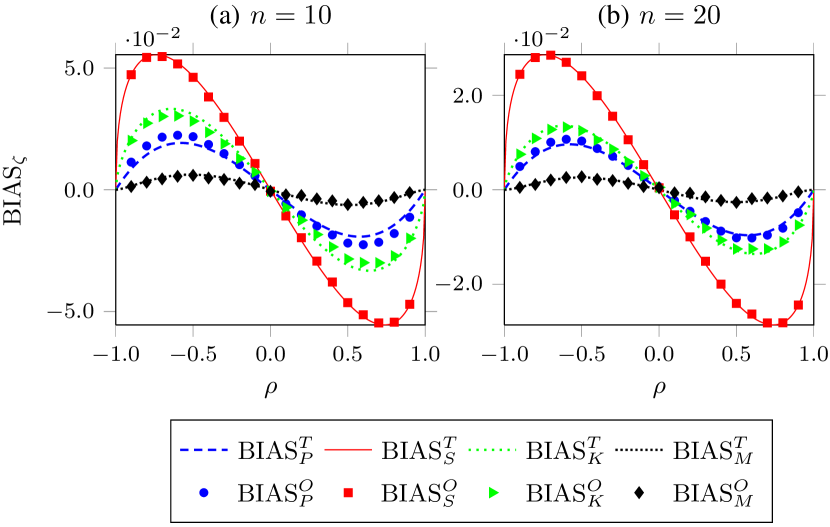
Figure 1: Comparison of $\mathrm{BIAS}_{\zeta}$, $\zeta\in\{P,S,K,M\}$ for (a) $n=10$ and (b) $n=20$. Theoretical curves, denoted by $\mathrm{BIAS}_{\zeta}^{T}$ in the legend, are plotted over $\rho=-1(0.01)1$ based on (48)–(51), respectively; whereas the simulation results, denoted by $\mathrm{BIAS}_{\zeta}^{O}$ in the legend, are plotted over $\rho=-0.9(0.1)0.9$.

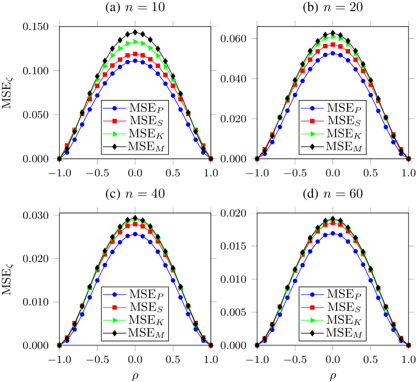
Figure 2: Comparison of observed $\mathrm{MSE}_{\zeta}$, $\zeta\in\{P,S,K,M\}$ for (a) $n=10$, (b) $n=20$, (c) $n=40$, and (d) $n=60$ over $\rho=-1(0.1)1$, respectively.

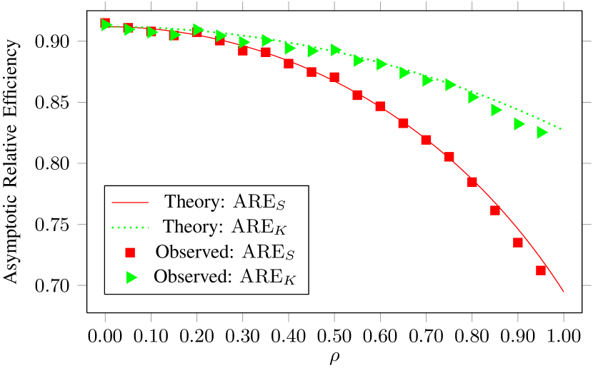
Figure 3: Verification and Comparison of $\mathrm{ARE}_{S}$ and $\mathrm{ARE}_{K}$ for $n=1000$ over $\rho=0(0.01)1$, for theoretical curves, and $\rho=0(0.05)0.95$, for simulation results. The results (64) and (65) are used to plot the two theoretical curves for $\rho=1$, respectively.

TABLE III: Variances of $\mathbb{V}(\hat{\rho}_{\zeta})$, $\zeta\in\{P,S,K,M\}$ for $n=10,20,30$

VI-B Verification of $\mathrm{BIAS}_{\zeta}$ and $\mathbb{V}(\hat{\rho}_{\zeta})$ in Small Samples

Fig. 1 shows the bias effects $\mathrm{BIAS}_{\zeta}$ corresponding to the four estimators $\rho_{\zeta}$, $\zeta\in\{P,S,K,M\}$ for $n=10$ and $n=20$, respectively. It is clearly observed that the magnitudes of $\mathrm{BIAS}_{\zeta}$ can be ordered as $\mathrm{BIAS}_{M}<\mathrm{BIAS}_{P}<\mathrm{BIAS}_{K}<\mathrm{BIAS}_{S}$. That is, the performance of $r_{S}$ is much worse than those of the other three in terms of bias effect in small samples. Moreover, it is also observed that (49) and (51) with respect to $\mathrm{BIAS}_{S}$ and $\mathrm{BIAS}_{M}$ are more accurate than (48) and (50) with respect to $\mathrm{BIAS}_{P}$ and $\mathrm{BIAS}_{K}$. In other words, the former two formulae agree better than do the latter two formulae with the corresponding simulation results for a sample size $n$ as small as $10$. Nevertheless, the deviations from (48) and (50) to the corresponding simulation results are less noticeable when the sample size $n$ is increased up to $20$.

Table III lists, for each of the three samples sizes, $10$, $20$ and $30$, 1) the theoretical results (55)–(58) with respect to $\mathbb{V}(\hat{\rho}_{\zeta})$ and 2) the corresponding observed variances from the Monte Carlo simulations. It can be seen that (56) and (58), with respect to $\mathbb{V}(\hat{\rho}_{S})$ and $\mathbb{V}(\hat{\rho}_{M})$, are accurate enough even though the sample size is as small as $n=10$. On the other hand, unfortunately, the theoretical formula (55) for $\mathbb{V}(\hat{\rho}_{P})$ and (57) for $\mathbb{V}(\hat{\rho}_{K})$ deviate substantially from the corresponding observed simulation results for the same sample size $n=10$. However, it appears that these deviations become less noticeable for $n=20$ and negligible for $n=30$. Therefore, it would be save to use (55)–(58) when approximating the variances of $\hat{\rho}_{\zeta}$ for $n\geq 20$ in practice.

VI-C Comparison of MSE in Small Samples

Contrary to $\mathrm{BIAS}_{\zeta}$ illustrated in Fig. 1, the magnitudes of the mean square errors

$$\mathrm{MSE}_{\zeta}\triangleq\mathbb{E}\left[(\hat{\rho}_{\zeta}-\rho)^{2}\right],\,\zeta\in\{P,S,K,M\}$$

cannot be ordered in a consistent manner. It appears in Fig. 2 that 1) $\mathrm{MSE}_{M}>\mathrm{MSE}_{K}>\mathrm{MSE}_{S}>\mathrm{MSE}_{P}$ when $|\rho|$ is around $0$, 2) $\mathrm{MSE}_{S}>\mathrm{MSE}_{K}>\mathrm{MSE}_{P}$ when $|\rho|$ exceeds some threshold, which moves towards $0$ with increase of $n$, and 3) the difference between $\mathrm{MSE}_{K}$ and $\mathrm{MSE}_{S}$ around $\rho=0$ decreases steadily with increase of $n$. Furthermore, due to the asymptotic equivalence between $\hat{\rho}_{S}$ and $\hat{\rho}_{M}$, $\mathrm{MSE}_{S}$ and $\mathrm{MSE}_{M}$ becomes closer and closer as $n$ increases.

VI-D Verification and Comparison of $\mathrm{ARE}_{S}$ and $\mathrm{ARE}_{K}$

Fig. 3 verifies and compares the performance of $\hat{\rho}_{S}$ and $\hat{\rho}_{K}$ in terms of ARE. For purpose of numerical verification, simulation results for $n=1000$ are superimposed upon the corresponding theoretical curves. Due to the asymptotic equivalence between $\hat{\rho}_{S}$ and $\hat{\rho}_{M}$, the results with respect to $\mathrm{ARE}_{M}$ are not included in Fig. 3. It can be observed that 1) the simulations agree well with our theoretical findings in (62) and (63), respectively, 2) $\mathrm{ARE}_{K}$ lies consistently above $\mathrm{ARE}_{S}$, indicating the superiority of $\hat{\rho}_{K}$ over $\hat{\rho}_{S}$ for large samples, and 3) the performance of $\hat{\rho}_{S}$ deteriorates severely as $\rho$ approaching unity, although it performs similarly as $\hat{\rho}_{K}$ when $\rho$ is small. Note that the remarks on $\mathrm{ARE}_{S}$ also apply to $\mathrm{ARE}_{M}$ due to the equivalence between $\hat{\rho}_{S}$ and $\hat{\rho}_{M}$ when the sample size $n$ is large.

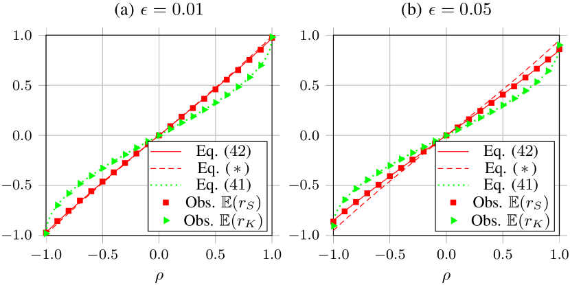
Figure 4: Verification of Theorem 3 for (a) $\epsilon=0.01$ and (b) $\epsilon=0.05$ under the sample size $n=50$ over $\rho=(-1)0.1(1)$, for simulations, and $\rho=(-1)0.01(1)$, for theoretical formulae (41) and (42). The rest parameters of the model (40) are set to be $\sigma_{X}=\sigma_{Y}=1$, $\lambda_{X}=\lambda_{Y}=100$ and $\rho^{\prime}=0$, respectively. The formula ($*$) concerning $\mathbb{E}(r_{S})$ developed elsewhere [21] is also included for comparison.

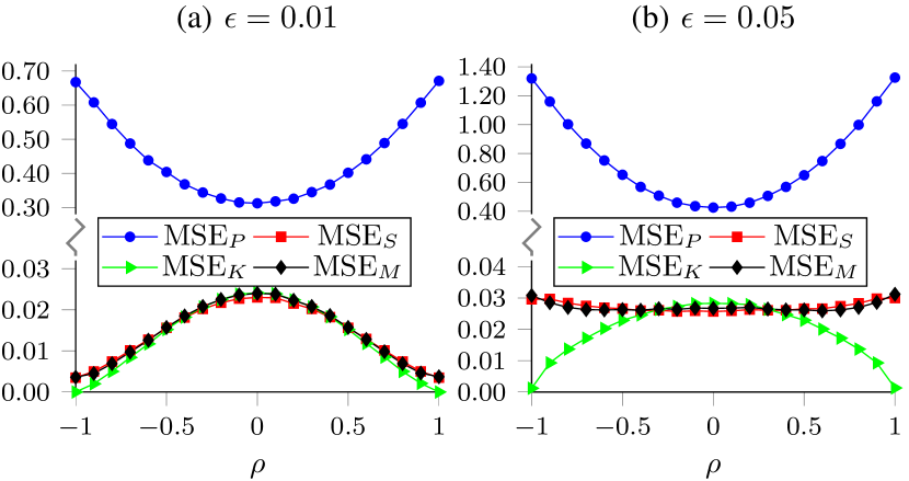
Figure 5: Performance comparison it terms of $\mathrm{MSE}_{\zeta}$, $\zeta\in\{S,P,K,M\}$, over $\rho=-1(0.1)1$ in the contaminated normal model (40) for (a) $\epsilon=0.01$ and (b) $\epsilon=0.05$ under the sample size $n=50$. The rest parameters of the model are set to be $\sigma_{X}=\sigma_{Y}=1$, $\lambda_{X}=\lambda_{Y}=100$ and $\rho^{\prime}=0$, respectively.

VI-E Performance of $\hat{\rho}_{\zeta}$ in Contaminated Normal Model

Fig. 4 puports to 1) verify the two statements concerning $\mathbb{E}(r_{K})$ and $\mathbb{E}(r_{S})$ in Theorem 3 under the contaminated Gaussian model (40), and 2) compare our formula (42) with the result of ($\ast$) that asserted in [21]. Due to the lack of space, we only present the results for $\epsilon=0.01$ and $\epsilon=0.05$ under the sample size $n=50$ here. For simplicity, the rest parameters of the model (40) are set to be $\sigma_{X}=\sigma_{Y}=1$, $\lambda_{X}=\lambda_{Y}=100$ and $\rho^{\prime}=0$ throughout. It is seen that the observed values of $\mathbb{E}(r_{K})$ and $\mathbb{E}(r_{S})$ agree well with the corresponding theoretical results of (41) and (42) established in Theorem 3. On the other hand, however, the curves with respect to ($\ast$), especially in Fig. 4(b), deviate obviously from the corresponding observed values.

Fig. 5 illustrates, in terms of MSE, the sensitivity of $\hat{\rho}_{P}$ as well as the robustness of $\hat{\rho}_{S}$, $\hat{\rho}_{K}$ and $\hat{\rho}_{M}$ to impulsive noise. It is shown in Fig. 5 that the MSE of $\hat{\rho}_{P}$ is dramatically larger than those of the other three estimators, irrespective of how small the fraction $\epsilon$ of impulsive component is. On the other hand, it is seen that, despite some minor negative (positive) differences for $\rho$ around $0$ ($\pm 1$), $\mathrm{MSE}_{S}$ and $\mathrm{MSE}_{M}$ behave similarly with $\mathrm{MSE}_{K}$ for $\epsilon=0.01$. Nevertheless, $\mathrm{MSE}_{S}$ and $\mathrm{MSE}_{M}$ are much larger than $\mathrm{MSE}_{K}$ for $\epsilon=0.05$ when $\rho$ falls in the neighborhood of $\pm 1$. Combing Fig. 5(a) and (b), it would be reasonable to rank their performance as $\hat{\rho}_{K}\geq\hat{\rho}_{S}\sim\hat{\rho}_{M}\gg\hat{\rho}_{P}$ in terms of MSE under the contaminated normal model (40), where the symbol $\sim$ stands for “is similar to”.

VII Concluding Remarks

In this paper we have investigated systematically the properties of the Spearman’s rho and Kendall’s tau for samples drawn from bivariate normal contained normal populations. Theoretical derivations along with Monte Carlo simulations reveal that, contrary to the opinion of equivalence between SR and KT in some literature, e.g. [23], they behave quite differently in terms of mathematical tractability, bias effect, mean square error, asymptotic relative efficiency in the normal cases and robustness properties in the contaminated normal model.

As shown in Theorem 1, SR is mathematically less tractable than KT, in the sense of the intractable terms $\Omega_{1}(\rho)$ and $\Omega_{2}(\rho)$ in the formula of its variance (20), in contrast with the closed form expression of $\mathbb{V}(r_{K})$ in (19). However, this mathematical inconvenience is, to some extent, offset by Table I provided in this work, especially from the viewpoint of numerical accuracy. Moreover, as demonstrated in Fig. 1 and Table III, the convergence speed of the asymptotic formulae (50) and (57) with respect to $\mathrm{BIAS}_{K}$ and $\mathbb{V}(\hat{\rho}_{K})$ are less accurate than those of $\mathrm{BIAS}_{S}$ and $\mathbb{V}(\hat{\rho}_{S})$ due to the high nonlinearity of the calibration (45). As a consequence, we do not attach too much importance to such mathematical advantage of KT over SR.

Now let us turn back to the question raised at the very beginning of this paper: which one, SR or KT, should we use in practice when PPMCC is inapplicable? The answer to this question is different for different requirements of the task at hand. Specifically,

1. If unbiasedness is on the top priority list, then neither $\hat{\rho}_{S}$ or $\hat{\rho}_{K}$ should be resorted to. The modified version $\hat{\rho}_{M}$ that employs both SR and KT, is definitely the best choice (cf. Fig. 1).

2. One the other hand, if minimal MSE is the critical feature and the sample size $n$ is small, then $\hat{\rho}_{S}$ ($\hat{\rho}_{K}$) should be employed when the population correlation $\rho$ is weak (strong) (cf. Fig. 2).

3. Since $\hat{\rho}_{K}$ outperforms $\hat{\rho}_{S}$ asymptotically in terms of ARE, then $\hat{\rho}_{K}$ is the suitable statistic in large-sample cases (cf. Fig. 3).

4. If their is impulsive noise in the data, then it would be better to employ $\hat{\rho}_{K}$, in terms of MSE, although there is some minor advantage of $\hat{\rho}_{S}$ when $\rho$ is in the neighborhood of $0$ (cf. Fig. 5).

5. Moreover, in terms of time complexity, $\hat{\rho}_{S}$ appears to be superior to $\hat{\rho}_{K}$—the computational load of the former is $O(n\log n)$; whereas and the computational load of the latter is $O(n^{2})$ [35].

Possessing the desirable properties summarized in Section II, Spearman’s rho and Kendall’s tau have found wide applications in the literature other than information theory. With the new insights uncovered in this paper, these two rank based coefficients can play complementary roles under the circumstances where Pearson’s product moment correlation coefficient is no longer effective.

Appendix A Proof of Theorem 1

TABLE IV: Quantities for evaluation of $\mathbb{E}(\mathcal{S}^{2})$ in Theorem 1

Proof:

Using the technique developed by Moran [44] for finding $\mathbb{E}(r_{S})$, it follows that the ranks can be expressed as

$$P_{i} =\sum_{j=1}^{n}H(X_{i}-X_{j})+1$$ (66)

$$Q_{i} =\sum_{k=1}^{n}H(Y_{i}-Y_{k})+1$$ (67)

where $H(\blacktriangle)$ is defined in (7). Substituting (66) and (67) into (2) yields

$$r_{S}=\frac{\mathcal{S}-\frac{1}{4}(n-1)^{2}}{n}\frac{12}{n^{2}-1}$$ (68)

where

$$\begin{split}\mathcal{S}&=\sum_{i=1}^{n}\sum_{j=1}^{n}\sum_{k=1}^{n}H(X_{i}-X_{j})H(Y_{i}-Y_{k})\\ &=\underset{i\neq j=1}{\sum\limits^{n}\sum\limits^{n}}H(X_{i}-X_{j})H(Y_{i}-Y_{j})\\ &\hskip 28.45274pt+\underset{i\neq j\neq k=1}{\sum\limits^{n}\sum\limits^{n}\sum\limits^{n}}H(X_{i}-X_{j})H(Y_{i}-Y_{k}).\end{split}$$ (69)

Then

$$\mathbb{V}(r_{S})=\frac{144}{n^{2}(n^{2}-1)^{2}}\underbrace{\bigg{[}\mathbb{E}(\mathcal{S}^{2})-\mathbb{E}^{2}(\mathcal{S})\bigg{]}}_{\mathbb{V}(\mathcal{S})}.$$ (70)

Taking the expectation of both sides of (69) with the assistance of (9) in Lemma 2, it follows readily that

$$\mathbb{E}(\mathcal{S})=n^{[2]}\left(\frac{1}{4}+\frac{S_{1}}{2\pi}\right)+n^{[3]}\left(\frac{1}{4}+\frac{S_{2}}{2\pi}\right)$$ (71)

where $n^{[\kappa]}\triangleq n(n{-}1)\cdots(n{-}\kappa{+}1)$, with $\kappa$ being a positive integer. Now the variance of $r_{S}$ depends on the evaluation of $\mathbb{E}(\mathcal{S}^{2})$, which is a weighted summation of $24$ quadrivariate normal orthant probabilities $P_{4}^{0}(R_{\xi})=\mathbb{E}(Z_{1}Z_{2}Z_{3}Z_{4})$ corresponding to $R_{\xi}$ listed in Table IV [29]. Collecting the terms of $P_{4}^{0}(R_{\xi})$ in Table IV, subtracting the square of the right side of (71) and substituting the resultant into (70) along with some simplifications, we obtain the expression of (20) with

$$\Omega_{1}(\rho) {=}W_{c}{+}4W_{d}{+}2W_{e}{+}2W_{f}$$ (72)

$$\Omega_{2}(\rho) {=}4(W_{g}{+}W_{h}{+}W_{l}{+}W_{q}){+}2(W_{n}{+}W_{p}){+}W_{m}{+}W_{o}.$$ (73)

An application of the relationship (11) to Appendix 2 of [29] yields

$$W_{e}{=}2W_{d},\,W_{g}{=}W_{p},\,W_{h}{=}W_{q},\text{ and }W_{m}{=}2W_{l}+\frac{1}{3}.$$ (74)

Substituting (74) into (72) and (73) yields (21) and (22), respectively. Hence the first theorem statement (20) follows. Ignoring the $o(n^{-1})$ terms in (20) yields the second statement (23), thus completing the proof. ∎

Appendix B Derivations of $\Omega_{1}(\rho)$, $\Omega_{2}(\rho)$ and $\Omega_{3}(\rho)$ for $\rho=0,1$

Proof:

From (21), (22) and (30), it suffices to evaluate $W_{\xi^{\prime}}$, $\xi^{\prime}\in\{c,d,f,g,h,l,n,o\}$ for $\rho=0,1$; and with (34), it suffices to evaluate $P_{4}^{0}(R_{\xi^{\prime}})$ for $\rho=0,1$. It follows readily from Appendix 2 of [29] that for $\rho=0$, $P_{4}^{0}(R_{c})=P_{4}^{0}(R_{g})=1/9$, $P_{4}^{0}(R_{d})=P_{4}^{0}(R_{h})=1/24$, $P_{4}^{0}(R_{f})=P_{4}^{0}(R_{o})=1/16$, $P_{4}^{0}(R_{l})=1/18$, $P_{4}^{0}(R_{n})=1/36$. Then, with the help of (34), we have the values $W_{\xi^{\prime}}(0)$ as listed in the $W(0)$-column of Table IV. Using these $W_{\xi^{\prime}}(0)$ values with the relationships (21), (22) and (30) yields $\Omega_{1}(0)=1/9$, $\Omega_{2}(0)=5/9$ and $\Omega_{3}(0)=1/18$, respectively.

When $\rho$ approaches unity, it is rather tricky to evaluate the values $W_{\xi^{\prime}}(1)$. Substituting $\rho=1$ directly into the integrals in (13) or the integrals in Appendix 2 of [29] will not lead to any tractable argument. We have to investigate case by case. From Table IV, it is seen that the off-diagonal elements of $R_{c}$ are all $1/2$ When $\rho=1$. Then we have $P_{4}^{0}(R_{c})|_{\rho=1}=1/5$ [46], and hence $W_{c}(1)=1/5$ by (34). From [47] it follows that $P_{4}^{0}(R_{f})|_{\rho=1}=2/15$ and $P_{4}^{0}(R_{m})|_{\rho=1}=1/6$. Then we have, by (34), $W_{f}(1)=2/15$ and $W_{m}(1)=1/3$, the latter yielding $W_{l}(1)=0$ from the identity $W_{m}=W_{l}+1/3$ in (74). Substituting $R_{f}|_{\rho=1}$ into (12) and exchanging $z_{1}$ and $z_{2}$ gives $W_{f}(1)=W_{e}(1)$, which implies that $W_{d}(1)=1/15$ by the identity $W_{e}=2W_{d}$ in (74). Similarly we also have $W_{o}(1)=W_{m}(1)=1/3$ upon substitution of $R_{m}|_{\rho=1}$ into (12) and exchange of $z_{3}$ and $z_{4}$. It is easy to verify that $P_{4}^{0}(R_{n})$ vanishes as $\rho\to 1$, since in this case $Z_{1}=-Z_{4}$ and $H(Z_{1})H(Z_{2})H(Z_{3})H(Z_{4})\equiv 0$ by the definition of H($\blacktriangle$) in (7). Then $W_{n}(1)=0$ by applying the relationship (34) once more. When $\rho$ approaches unity, it follows that $P_{4}^{0}(R_{g})$ and $P_{4}^{0}(R_{h})$ degenerate to two trivariate normal orthant probabilities that have closed form expressions (10). Specifically, it follows that $P_{4}(R_{g})_{\rho\to 1}=1/4$ and $P_{4}(R_{h})|_{\rho\to 1}=1/8$, yielding $W_{g}(1)=1/3$ and $W_{h}(1)=1/3$, respectively. Having all the values of $W_{\xi^{\prime}}(1)$, as listed in the $W(1)$-column of Table IV, and the three relationships (21), (22) and (30), we obtain $\Omega_{1}(1)=1$, $\Omega_{2}(1)=16/3$ and $\Omega_{3}(1)=1/2$, respectively, and the evaluations complete. ∎

Appendix C Proof of Theorem 2

TABLE V: Quantities for evaluation of $\mathbb{E}(\mathcal{S}\mathcal{T})$ in Theorem 2

Proof:

Let $\mathcal{S}$ be the same as in (69) and $\mathcal{T}$ be the numerator of (3). Define

$$I \triangleq\underset{i\neq j}{\sum}\,H(X_{i}-X_{j})H(Y_{i}-Y_{j})$$ (75)

$$J \triangleq\underset{i\neq j\neq k}{\sum}H(X_{i}-X_{j})H(Y_{i}-Y_{k})$$ (76)

$$K \triangleq\underset{i\neq j}{\sum}\,H(X_{i}-X_{j})$$ (77)

$$L \triangleq\underset{i\neq k}{\sum}\,H(Y_{i}-Y_{k}).$$ (78)

Then, we have, from (3), (68) and (69) along with the relationship $\mathrm{sgn}(\blacktriangle)=2H(\blacktriangle)-1$,

$$\mathcal{S} =I+J$$ (79)

$$\mathcal{T} =4I-2K-2L+n^{[2]}$$ (80)

and hence

$$\begin{split}\mathbb{C}(r_{S},r_{K})&=\frac{12}{n^{2}(n-1)(n^{2}-1)}\mathbb{C}(\mathcal{S},\mathcal{T})\\ &=\frac{12}{n^{2}(n-1)(n^{2}-1)}\bigg{[}\mathbb{E}(\mathcal{S}\mathcal{T})-\mathbb{E}(\mathcal{S})\mathbb{E}(\mathcal{T})\bigg{]}.\end{split}$$ (81)

From (1) and (9), it follows that

$$\mathbb{E}(I)=n^{[2]}\left(\frac{1}{4}+\frac{S_{1}}{2\pi}\right)\text{ and }\mathbb{E}(K)=\mathbb{E}(L)=\frac{n^{[2]}}{2}.$$

Substituting these expectation terms into (80) gives

$$\mathbb{E}(\mathcal{T})=4n^{[2]}\left(\frac{1}{4}+\frac{S_{1}}{2\pi}\right)-n^{[2]}=\frac{2n^{[2]}}{\pi}S_{1}.$$ (82)

Recall that we have obtained $\mathbb{E}(\mathcal{S})$ in (71). Now the only difficulty lies in the evaluation of $\mathbb{E}(\mathcal{S}\mathcal{T})$ in (81). Multiplying (79) and (80), expanding and taking expectations term by term, we have

$$\begin{split}\mathbb{E}(\mathcal{S}\mathcal{T})&=4\mathbb{E}(IJ)-2\mathbb{E}(KJ)-2\mathbb{E}(LJ)\\ &\quad+4\mathbb{E}(I^{2})-2\mathbb{E}(KI)-2\mathbb{E}(LI)+n^{[2]}\mathbb{E}(\mathcal{S}).\end{split}$$ (83)

Now, resorting to Table V, we are ready to evaluate the first six terms in (83). From (75) and (76), it follows that $\mathbb{E}(IJ)$ is a summation of $P_{4}^{0}$ terms of the form

$$\mathbb{E}\{H(\underbrace{X_{i}{-}X_{j}}_{Z_{1}})H(\underbrace{Y_{i}{-}Y_{j}}_{Z_{2}})H(\underbrace{X_{k}{-}X_{l}}_{Z_{3}})H(\underbrace{Y_{k}{-}Y_{m}}_{Z_{4}})\}.$$ (84)

Since, by definition (7), $H(0)=0$, the term (84) vanishes for $i=j$ or $k=l$ or $k=m$. Then there are $n^{2}(n-1)^{2}(n-2)$ nontrivial (84)-like terms left to be evaluated. It follows that the domain of the quintuple $(i,j,k,l,m)$ can be partitioned into thirteen disjoint and exhaustive subsets whose representative terms, $Z_{1}$, $Z_{2}$, $Z_{3}$, $Z_{4}$, are listed in the upper panel of Table V. Summing up the corresponding $P_{4}^{0}$-terms in Table V leads directly to $\mathbb{E}(IJ)$. In a similar manner we can obtain $\mathbb{E}(KJ)$ and $\mathbb{E}(LJ)$. With the assistance of the lower panel of Table V, we also have the expressions of $\mathbb{E}(I^{2})$, $\mathbb{E}(KI)$ and $\mathbb{E}(LI)$. Substituting these results and (71) into (83), subtracting the multiplication of (71) and (82) and substituting the resultant back into (81), we find that $\mathbb{C}(r_{S},r_{K})$ is of the form (28) with

$$\Omega_{3}(\rho)=\frac{1}{4}W_{g}+\frac{1}{4}W_{p}+\frac{1}{2}W_{h}+\frac{1}{2}W_{q}$$

which simplifies to (30) by applying the identities in (74). The theorem then follows. ∎

Appendix D Proof of Theorem 3

Proof:

For ease of the following discussion, we will use $\phi(x,y)$ and $\psi(x,y)$ to denote the pdfs of the two bivariate normal components in (40), respectively. From (66), (67) and (80), it follows that the numerator of (3) $\mathcal{T}$ can be simplified to

$$\mathcal{T}=4\underset{i\neq j=1}{\sum\limits^{n}\sum\limits^{n}}H(X_{i}-X_{j})H(Y_{i}-Y_{j})-n^{[2]}$$ (85)

which yields

$$\mathbb{E}(\mathcal{T})=4n^{[2]}\underbrace{\mathbb{E}\left[H(X_{1}-X_{2})H(Y_{1}-Y_{2})\right]}_{E_{1}}-n^{[2]}$$ (86)

by the i.i.d. assumption. To evaluate $E_{1}$ in (86), we need the joint distribution of $(X_{1},Y_{1},X_{2},Y_{2})$, denoted by $\varphi(x_{1},y_{1},x_{2},y_{2})$, which is readily obtained as

$$\begin{split}\varphi&=\left[(1-\epsilon)\phi_{1}+\epsilon\psi_{1}\right]\left[(1-\epsilon)\phi_{2}+\epsilon\psi_{2}\right]\\ &=\underbrace{(1{-}\epsilon)^{2}}_{\alpha_{1}}\underbrace{\phi_{1}\phi_{2}}_{\varphi_{1}}{+}\underbrace{\epsilon(1{-}\epsilon)}_{\alpha_{2}}\underbrace{\phi_{1}\psi_{2}}_{\varphi_{2}}{+}\underbrace{\epsilon(1{-}\epsilon)}_{\alpha_{3}}\underbrace{\phi_{2}\psi_{1}}_{\varphi_{3}}{+}\underbrace{\epsilon^{2}}_{\alpha_{4}}\underbrace{\psi_{1}\psi_{2}}_{\varphi_{4}}\end{split}$$ (87)

where $\varphi$, $\phi_{i}$, $\psi_{i}$ are compact notations of $\varphi(x_{1},y_{1},x_{2},y_{2})$, $\phi(x_{i},y_{i})$ and $\psi(x_{i},y_{i})$, $i=1,2$, respectively. Write

$$U\triangleq\frac{X_{1}-X_{2}}{\sqrt{\mathbb{V}(X_{1}-X_{2})}}\text{ and }V\triangleq\frac{Y_{1}-Y_{2}}{\sqrt{\mathbb{V}(Y_{1}-Y2)}}.$$

Then, with respect to $\varphi_{1}$, $\varphi_{2}$, $\varphi_{3}$, and $\varphi_{4}$ in (87), $(U,V)$ follows four standard bivariate normal distributions with correlations

$$\varrho_{1} =\rho$$ (88)

$$\varrho_{2} =\frac{\rho+\lambda_{X}\lambda_{Y}\rho^{\prime}}{\sqrt{1+\lambda_{X}^{2}}\sqrt{1+\lambda_{Y}^{2}}}\to\rho^{\prime}\text{ as }\lambda_{X},\lambda_{Y}\to\infty$$ (89)

$$\varrho_{3} =\frac{\rho+\lambda_{X}\lambda_{Y}\rho^{\prime}}{\sqrt{1+\lambda_{X}^{2}}\sqrt{1+\lambda_{Y}^{2}}}\to\rho^{\prime}\text{ as }\lambda_{X},\lambda_{Y}\to\infty$$ (90)

$$\varrho_{4} =\rho^{\prime}$$ (91)

respectively. An application of the Sheppard’s theorem (9) to (86) along with (88)–(91) yields

$$\begin{split}\mathbb{E}(\mathcal{T})&=4n^{[2]}\sum_{i=1}^{4}\alpha_{i}\left(\frac{1}{4}+\frac{1}{2\pi}\sin^{-1}\varrho_{i}\right)-n^{[2]}\\ &=\frac{2n^{[2]}}{\pi}\left[\alpha_{1}\sin^{-1}\rho{+}2\alpha_{2}\sin^{-1}\varrho_{2}{+}\alpha_{4}\sin^{-1}\rho^{\prime}\right].\end{split}$$ (92)

Now it is not difficult to verify that the first statement (41) holds by 1) dividing both sides of (92) by $n^{[2]}$, 2) letting $\lambda_{X}\to\infty$ and $\lambda_{Y}\to\infty$, and 3) ignoring the $O(\epsilon^{2})$ terms.

To prove the second statement (42), it suffices to evaluate $\mathbb{E}(\mathcal{S})$ by the relationship (68). Taking expectations of both sides in (69) along with the i.i.d. assumptions gives

$$\mathbb{E}(\mathcal{S})=n^{[2]}E_{1}+n^{[3]}\underbrace{\mathbb{E}\left[H(X_{1}-X_{2})H(Y_{1}-Y_{3})\right]}_{E_{2}}.$$ (93)

Since we have known $E_{1}$ in the above development, now we only need to work out $E_{2}$ in (93). Let $\varpi(x_{1},y_{1},x_{2},y_{2},x_{3},y_{3})$, abbreviated as $\varpi$, denote the pdf of the joint distribution of $(X_{1},Y_{1},X_{2},Y_{2},X_{3},Y_{3})$. Then, from (40) and the i.i.d. assumption,

$$\begin{split}\varpi&=\left[(1{-}\epsilon)\phi_{1}{+}\epsilon\psi_{1}\right]\left[(1{-}\epsilon)\phi_{2}{+}\epsilon\psi_{2}\right]\left[(1{-}\epsilon)\phi_{3}{+}\epsilon\psi_{3}\right]\\ &=(1{-}\epsilon)^{3}\underbrace{\phi_{1}\phi_{2}\phi_{3}}_{\varpi_{1}}{+}\epsilon(1{-}\epsilon)^{2}(\underbrace{\phi_{1}\phi_{2}\psi_{3}}_{\varpi_{2}}{+}\underbrace{\phi_{1}\psi_{2}\phi_{3}}_{\varpi_{3}}{+}\underbrace{\psi_{1}\phi_{2}\phi_{3}}_{\varpi_{4}})\\ &\phantom{=}+\epsilon^{2}(1{-}\epsilon)(\underbrace{\phi_{1}\psi_{2}\psi_{3}}_{\varpi_{5}}{+}\underbrace{\psi_{1}\phi_{2}\psi_{3}}_{\varpi_{6}}{+}\underbrace{\psi_{1}\psi_{2}\phi_{3}}_{\varpi_{7}})+\epsilon^{3}\underbrace{\psi_{1}\psi_{2}\psi_{3}}_{\varpi_{8}}.\end{split}$$ (94)

where $\phi_{i}$ and $\psi_{i}$ are compact notations of $\phi(x_{i},y_{i})$ and $\psi(x_{i},y_{i})$, $i=1,2,3$, respectively. Define

$$V^{\prime}=\frac{Y_{1}-Y_{3}}{\sqrt{\mathbb{V}(Y_{1}-Y_{3})}}.$$

Then, with respect to $\varpi_{1}$ to $\varpi_{8}$ in (94), $(U,V^{\prime})$ follows $8$ standard bivariate normal distributions with correlations

$$\varrho_{5} =\frac{\rho}{2}$$ (95)

$$\varrho_{6} =\frac{1}{\sqrt{2}}\frac{\rho}{\sqrt{1+\lambda_{Y}^{2}}}\to 0\text{ as }\lambda_{Y}\to\infty$$ (96)

$$\varrho_{7} =\frac{1}{\sqrt{2}}\frac{\rho}{\sqrt{1+\lambda_{X}^{2}}}\to 0\text{ as }\lambda_{X}\to\infty$$ (97)

$$\varrho_{8} =\frac{\lambda_{X}\lambda_{Y}\rho^{\prime}}{\sqrt{1+\lambda_{X}^{2}}\sqrt{1+\lambda_{Y}^{2}}}\to\rho^{\prime}\text{ as }\lambda_{X},\lambda_{Y}\to\infty$$ (98)

$$\varrho_{9} =\frac{\rho}{\sqrt{1+\lambda_{X}^{2}}\sqrt{1+\lambda_{Y}^{2}}}\to 0\text{ as }\lambda_{X},\lambda_{Y}\to\infty$$ (99)

$$\varrho_{10} =\frac{1}{\sqrt{2}}\frac{\lambda_{X}\rho^{\prime}}{\sqrt{1+\lambda_{X}^{2}}}\to\frac{\rho^{\prime}}{\sqrt{2}}\text{ as }\lambda_{X}\to\infty$$ (100)

$$\varrho_{11} =\frac{1}{\sqrt{2}}\frac{\lambda_{Y}\rho^{\prime}}{\sqrt{1+\lambda_{Y}^{2}}}\to\frac{\rho^{\prime}}{\sqrt{2}}\text{ as }\lambda_{Y}\to\infty$$ (101)

$$\varrho_{12} =\frac{\rho^{\prime}}{2}.$$ (102)

Using the Sheppard’s theorem (9) again together with (94)–(102), we can obtain the expression of $E_{2}$ and hence $\mathbb{E}(\mathcal{S})$ in terms of $n$, $\epsilon$ and $\varrho_{1}$ to $\varrho_{12}$. Substituting $\mathbb{E}(\mathcal{S})$ into (68), letting $n$, $\lambda_{X}$, $\lambda_{Y}\to\infty$ and ignoring the $O(\epsilon^{2})$ terms, we arrive at (42), the second theorem statement. ∎

Weichao Xu (M’06) received the B.Eng. and M.Eng. degrees in electrical engineering from the University of Science and Technology of China, Hefei, China, in 1993 and 1996, respectively. He received the Ph.D. degree in biomedical engineering from the University of Hong Kong, Hong Kong, in 2002. Since 2003, he has been a Research Associate with the Department of Electrical and Electronic Engineering, the University of Hong Kong. His research interests are in the areas of mathematical statistics, machine learning, digital signal processing and applications.

Yunhe Hou Yunhe Hou (M’06) received the B.E (1999), M.E(2002) and Ph.D(2005) degrees from the Huazhong University of Science and Technology, China. He worked as a postdoctoral research fellow at Tsinghua University from 2005 to 2007. He was a visiting scholar at Iowa State University, Ames, and a researcher of University College Dublin, Ireland from 2008 to 2009. He is currently with the University of Hong Kong, Hong Kong, as a research assistant professor.

Y. S. Hung (M’88–SM’02) received the B.Sc. (Eng.) degree in electrical engineering and the B.Sc. degree in mathematics from the University of Hong Kong, Hong Kong, and the M.Phil. and Ph.D. degrees from the University of Cambridge, Cambridge, U.K. He was a Research Associate with the University of Cambridge and a Lecturer with the University of Surrey, Surrey, U.K. In 1989, he joined the University of Hong Kong, where he is currently a Professor. His research interests include robust control systems theory, robotics, computer vision, and biomedical engineering. Prof. Hung was a recipient of the Best Teaching Award in 1991 from the Hong Kong University Students Union. He is a chartered engineer and a fellow of IET and HKIE.

Yuexian Zou Yuexian Zou received her M.Sc. (1991) and Ph.D. (2000) from the University of Electronic Science and Technology of China and the University of Hong Kong, respectively. Since 2006, she serves as an Associate Professor in Peking University, and is the director of the Advanced Digital Signal Processing Lab of Peking University Shenzhen Graduate School. Dr. Zou has more than 15 years research experience in digital signal processing, adaptive signal processing and their applications. She is currently the senior IEEE member and has published more than 50 journal and conference papers. She was the organization co-chair of NEMS09 and served as the founding chair of the WIE Singapore in 2005. She has carried out more than 10 national funded projects since 2000. She is currently working on a project funded by Shenzhen Bureau of Science Technology and Information in fast extraction of Somatosensory Evoked Potential. Dr. Zou s research interests include adaptive signal processing, biomedical signal processing and active noise control.

References

- [1] D. Ruchkin, “Error of correlation coefficient estimates from polarity coincidences (corresp.),” IEEE Trans. Inf. Theory, vol. 11, no. 2, pp. 296–297, Apr. 1965.
- [2] M. C. Cheng, “The clipping loss in correlation detectors for arbitrary input signal-to-noise ratios,” IEEE Trans. Inf. Theory, vol. 14, no. 3, pp. 382–389, May 1968.
- [3] H. Chadwick and L. Kurz, “Rank permutation group codes based on kendall’s correlation statistic,” IEEE Trans. Inf. Theory, vol. 15, no. 2, pp. 306–315, Mar. 1969.
- [4] V. Hansen, “Detection performance of some nonparametric rank tests and an application to radar,” IEEE Trans. Inf. Theory, vol. 16, no. 3, pp. 309–318, May 1970.
- [5] G. Goldstein, “Locally best unbiased estimation of the correlation coefficient in a bivariate normal population (corresp.),” IEEE Trans. Inf. Theory, vol. 19, no. 3, pp. 363–364, May 1973.
- [6] N. Bershad and A. Rockmore, “On estimating signal-to-noise ratio using the sample correlation coefficient (corresp.),” IEEE Trans. Inf. Theory, vol. 20, no. 1, pp. 112–113, Jan. 1974.
- [7] J. Bae, H. Kwon, S. R. Park, J. Lee, and I. Song, “Explicit correlation coefficients among random variables, ranks, and magnitude ranks,” IEEE Trans. Inf. Theory, vol. 52, no. 5, pp. 2233–2240, May 2006.
- [8] A. Johansen, T. Helleseth, and X. Tang, “The correlation distribution of quaternary sequences of period ,” IEEE Trans. Inf. Theory, vol. 54, no. 7, pp. 3130–3139, Jul. 2008.
- [9] A. Johansen and T. Helleseth, “A family of m-sequences with five-valued cross correlation,” IEEE Trans. Inf. Theory, vol. 55, no. 2, pp. 880–887, Feb. 2009.
- [10] K. Gomadam and S. Jafar, “The effect of noise correlation in amplify-and-forward relay networks,” IEEE Trans. Inf. Theory, vol. 55, no. 2, pp. 731–745, Feb. 2009.
- [11] A. Stuart and J. K. Ord, Kendall’s Advanced Theory of Statistics: Volume 2 Classical Inference and Relationship, 5th ed. London: Edward Arnold, 1991.
- [12] J. D. Gibbons and S. Chakraborti, Nonparametric Statistical Inference, 3rd ed. New York: M. Dekker, 1992.
- [13] R. A. Fisher, “On the ’probable error’ of a coefficient of correlation deduced from a small sample,” Metron, vol. 1, pp. 3–32, 1921.
- [14] ——, Statistical Methods, Experimental Design, and Scientific Inference. New York: Oxford University Press, 1990.
- [15] M. Kendall and J. D. Gibbons, Rank Correlation Methods, 5th ed. New York: Oxford University Press, 1990.
- [16] D. D. Mari and S. Kotz, Correlation and Dependence. London: Imperial College Press, 2001.
- [17] S. Tumanski, Principles of Electrical Measurement. New York: Taylor & Francis, 2006.
- [18] D. Stein, “Detection of random signals in gaussian mixture noise,” IEEE Trans. Inf. Theory, vol. 41, no. 6, pp. 1788–1801, Nov. 1995.
- [19] R. Chen, X. Wang, and J. Liu, “Adaptive joint detection and decoding in flat-fading channels via mixture Kalman filtering,” IEEE Trans. Inf. Theory, vol. 46, no. 6, pp. 2079–2094, Sep. 2000.
- [20] Z. Reznic, R. Zamir, and M. Feder, “Joint source-channel coding of a gaussian mixture source over the gaussian broadcast channel,” IEEE Trans. Inf. Theory, vol. 48, no. 3, pp. 776–781, Mar. 2002.
- [21] G. L. Shevlyakov and N. O. Vilchevski, Robustness in Data Analysis : criteria and methods, ser. Modern probability and statistics. Utrecht: VSP, 2002.
- [22] E. C. Fieller, H. O. Hartley, and E. S. Pearson, “Tests for rank correlation coefficients. i,” Biometrika, vol. 44, no. 3/4, pp. 470–481, Dec. 1957.
- [23] A. R. Gilpin, “Table for conversion of kendall’s tau to spearman’s rho within the context of measures of magnitude of effect for meta-analysis,” Educ. Psychol. Meas., vol. 53, no. 1, pp. 87–92, Mar. 1993.
- [24] A. Lapidoth and S. Tinguely, “Sending a bivariate gaussian source over a gaussian mac with feedback,” Information Theory, IEEE Transactions on, vol. 56, no. 4, pp. 1852–1864, Apr. 2010.
- [25] ——, “Sending a bivariate gaussian over a gaussian mac,” IEEE Trans. Inf. Theory, vol. 56, no. 6, pp. 2714–2752, Jun. 2010.
- [26] S. Bross, A. Lapidoth, and S. Tinguely, “Broadcasting correlated gaussians,” IEEE Trans. Inf. Theory, vol. 56, no. 7, pp. 3057–3068, Jul. 2010.
- [27] M. G. Kendall, “Rank and product-moment correlation,” Biometrika, vol. 36, no. 1/2, pp. 177–193, Jun. 1949.
- [28] S. T. David, M. G. Kendall, and A. Stuart, “Some questions of distribution in the theory of rank correlation,” Biometrika, vol. 38, no. 1/2, pp. 131–140, Jun. 1951.
- [29] F. N. David and C. L. Mallows, “The variance of spearman’s rho in normal samples,” Biometrika, vol. 48, no. 1/2, pp. 19–28, Jun. 1961.
- [30] W. Hoeffding, “A class of statistics with asymptotically normal distribution,” The Annals of Mathematical Statistics, vol. 19, no. 3, pp. 293–325, Sep. 1948.
- [31] H. E. Daniels, “The relation between measures of correlation in the universe of sample permutations,” Biometrika, vol. 33, no. 2, pp. 129–135, Aug. 1944.
- [32] ——, “Rank correlation and population models,” Journal of the Royal Statistical Society. Series B (Methodological), vol. 12, no. 2, pp. 171–191, 1950.
- [33] J. Durbin and A. Stuart, “Inversions and rank correlation coefficients,” Journal of the Royal Statistical Society. Series B (Methodological), vol. 13, no. 2, pp. 303–309, 1951.
- [34] W. Xu, C. Chang, Y. Hung, S. Kwan, and P. Fung, “Order statistic correlation coefficient and its application to association measurement of biosignals,” Proc. Int. Conf. Acoustics, Speech, Signal Process. (ICASSP) 2006, vol. 2, pp. II–1068–II–1071, May 2006.
- [35] W. Xu, C. Chang, Y. Hung, S. Kwan, and P. Chin Wan Fung, “Order statistics correlation coefficient as a novel association measurement with applications to biosignal analysis,” IEEE Trans. Signal Process., vol. 55, no. 12, pp. 5552–5563, dec. 2007.
- [36] W. Xu, C. Chang, Y. Hung, and P. Fung, “Asymptotic properties of order statistics correlation coefficient in the normal cases,” IEEE Trans. Signal Process., vol. 56, no. 6, pp. 2239–2248, Jun. 2008.
- [37] E. Schechtman and S. Yitzhaki, “A measure of association base on Gini’s mean difference,” Commun. Statist.-Theor. Meth., vol. 16, no. 1, pp. 207–231, 1987.
- [38] W. Xu, Y. S. Hung, M. Niranjan, and M. Shen, “Asymptotic mean and variance of Gini correlation for bivariate normal samples,” IEEE Trans. Signal Process., vol. 58, no. 2, pp. 522–534, Feb. 2010.
- [39] R. J. Serfling, Approximation Theorems of Mathematical Statistics, ser. Wiley series in probability and mathematical statistics. New York: Wiley, 2002.
- [40] A. Stuart, J. K. Ord, and S. F. Arnold, Kendall’s Advanced Theory of Statistics: Volume 1 Distribution Theory, 6th ed. London: Edward Arnold, 1994.
- [41] S. S. Gupta, “Probability integrals of multivariate normal and multivariate t,” The Annals of Mathematical Statistics, vol. 34, no. 3, pp. 792–828, Sep. 1963.
- [42] D. R. Childs, “Reduction of the multivariate normal integral to characteristic form,” Biometrika, vol. 54, no. 1/2, pp. 293–300, Jun. 1967.
- [43] H. Hotelling, “New light on the correlation coefficient and its transforms,” Journal of the Royal Statistical Society. Series B (Methodological), vol. 15, no. 2, pp. 193–232, 1953.
- [44] P. A. P. Moran, “Rank correlation and product-moment correlation,” Biometrika, vol. 35, no. 1/2, pp. 203–206, May 1948.
- [45] F. Esscher, “On a method of determining correlation from the ranks of the variates,” Skand. Aktuar., vol. 7, pp. 201–219, 1924.
- [46] G. P. Steck, “Orthant probabilities for the equicorrelated multivariate normal distribution,” Biometrika, vol. 49, no. 3/4, pp. 433–445, Dec. 1962.
- [47] R. L. Plackett, “A reduction formula for normal multivariate integrals,” Biometrika, vol. 41, no. 3/4, pp. 351–360, Dec. 1954.