Likelihood inference for particle location in fluorescence microscopy

Abstract

We introduce a procedure to automatically count and locate the fluorescent particles in a microscopy image. Our procedure employs an approximate likelihood estimator derived from a Poisson random field model for photon emission. Estimates of standard errors are generated for each image along with the parameter estimates, and the number of particles in the image is determined using an information criterion and likelihood ratio tests. Realistic simulations show that our procedure is robust and that it leads to accurate estimates, both of parameters and of standard errors. This approach improves on previous ad hoc least squares procedures by giving a more explicit stochastic model for certain fluorescence images and by employing a consistent framework for analysis.

T1Supported by the NSF/NIH joint initiative in mathematical biology DMS-07-14939.

, and

1 Introduction

The accurate and precise tracking of microscopic fluorescent particles attached to biological specimens (e.g., organelles, membrane proteins, molecular motors) can give insights into the nanoscale function and dynamics of those specimens. This tracking is accomplished by analyzing digital images produced by a CCD (charge-coupled device) camera attached to a microscope used to observe the specimens repeatedly. In this paper we introduce an improved technique for analyzing such images over time. Our method, which applies maximum likelihood principles, improves the fit to the data, derives accurate standard errors from the data with minimal computation, and uses model-selection criteria to “count” the fluorophores in an image. The ability to automate the process and quickly derive standard errors should allow for the analysis of thousands of images obtained from a typical experiment and aid in methods to track individual fluorophores across sequential images.

In fluorescence microscopy, a specimen of interest is tagged with a fluorescent molecule or particle. The fluorescence microscope then irradiates the specimen with light at the excitation wavelength of the fluorophore, and when the excited electrons revert to the ground state they emit photons at the emission wavelength. A filter separates the emitted light from the excitation light so that only the light from the fluorescent material can pass to the microscope’s eyepiece and camera system [Rost (1992)].

In general, the Rayleigh criterion implies that the maximum resolution for a light microscope should be roughly 250 nm (half of the wavelength of visible light); however, Selvin and his collaborators found that by fitting the center point of the point spread function one can locate a particle of interest. This technique is known as FIONA (Fluorescence Imaging with One-Nanometer Accuracy) and was introduced in Yildiz et al. (2003). The key element of FIONA is to focus attention on single fluorophores used as markers in biological specimens [Kural, Balci and Selvin (2005)]. By analyzing sequences of images, molecular motors (e.g., myosin VI and kinesin) and other specimens can be tracked through time, giving researchers insight into their dynamics and biological function. For instance, Yildiz et al. used FIONA to find compelling support for the hypothesis that myosin V walks hand over hand and evidence to eliminate other hypotheses [Yildiz et al. (2003); Kural, Balci and Selvin (2005)].

A number of analysis techniques have been proposed for FIONAimages. In 2001, Cheezum, Walker and Guilford compared fourmethods—cross-correlation, sum-absolute difference, centroid, and Gaussian fit—and ultimately recommended the Gaussian-fit method for single-fluorophore tracking. In the Gaussian-fit approach, the method of ordinary least squares (OLS) is used to fit a sum of symmetric bivariate Gaussian functions to the image. Least squares fitting is relatively efficient, and software to do it is widely available. Thompson, Larson and Webb subsequently proposed a “Gaussian mask” algorithm that is easier to implement than the Gaussian-fit method, is computationally less intensive, and performs nearly as well in simulations (2002). The Gaussian-mask algorithm is essentially a centroid calculation that weights each pixel with the number of photons in the pixel and with a bivariate Gaussian function integrated over the pixel. In both cases, simulation studies using typical experimental values showed that sub-pixel or even nanometer resolution was possible.

The above mentioned Gaussian-fit and Gaussian-mask methods, while appealing, share two shortcomings. Since one or more beads may move out of frame for a particular image, the number of beads from one image to the next is not known a priori and must be determined for each image. Previous authors have attempted to solve this problem by means of a grid search, the first step of which is to scan the image for all pixels greater than some arbitrary threshold value. Each of these extreme pixels is taken to be a bead location, and some region surrounding each extreme pixel is extracted from the image and processed by OLS or the Gaussian mask. Thompson et al. suggest a threshold that is eight standard deviations above the mean pixel value, but no explicit evidence is given in support of this choice [Thompson, Larson and Webb (2002)]. The correct threshold level for a set of images could possibly be approximated using simulations, but this would be a complex and computationally intensive task that would be necessary for each set of images, since the level of background noise may vary significantly from one experiment to the next.

The second drawback is that estimates of precision are derived from simulation studies alone. If the probability model for the problem is misspecified, then error estimates based on simulations from that model will be inaccurate even if reasonable parameter values were used in the studies. And these values will vary from image to image due to changing experimental conditions, for example, elevated background noise or slight changes in focus. A possible solution is to perform a Monte Carlo simulation study using parameter values derived from the current experiment. But, given that the fitting procedures themselves are time consuming, these approaches to standard error calculation may prove infeasible. It takes our algorithm several minutes—on a dual 2.8GHz Quad-Core Intel Xeon Mac Pro—to process an image with fifteen particles, which implies that bootstrapping standard errors for such an image would require hours of computation. Moreover, a full analysis of an experiment requires processing many hundreds of images.

In what follows we present a new approach to counting and locating fluorophores. Our approach eliminates the need for a grid search and estimates standard errors from the data, without additional simulation, via standard likelihood tools. In Section 2 we present an explicit probability model for a FIONA image along with a maximum likelihood estimation procedure suitable for this model. In Section 3 we discuss the properties of the approximate likelihood estimator presented in Section 2. In Section 4 we discuss stepwise model selection, which allows our procedure to automatically determine the number of beads in an image in a consistent manner. In Section 5 we describe the results of realistic simulation studies that support the approximations presented in Section 2 and demonstrate the robustness of our procedure. Finally, in Section 6 we carry out a complete analysis of an experimentally collected FIONA image, introducing relevant diagnostic criteria for our fit.

2 Model for data from a single FIONA image

We first develop a model for the photon emission from particles distributed over a microscope slide. Photon emission from a constant source generally follows a Poisson distribution; this fact naturally leads to a Poisson random field model for the emission from a slide. We then express the effect of pixelation on the field, representing the emission as viewed from the digital camera, and employ a normal approximation to the Poisson distribution. We arrive at our final approximate model by accounting for additional error introduced by the camera and its associated equipment.

We begin with the standard model for the photon-emission pattern (as distorted by the point-spread function of a microscope objective) of a collection of fluorophores distributed at random over some region of $\mathbb{R}^{2}$ [Cheezum, Walker and Guilford (2001); Thompson, Larson and Webb (2002)].

Let $N$, a Poisson random field on a rectangular subset $T$ of $\mathbb{R}^{2}$, represent the emission pattern of the sample. The intensity function can be defined for any Borel set $R\subset T$ as

$$\ \,E\{N(R)\}=\int\int_{R}\Biggl{\{}B+\sum\limits_{j=0}^{J-1}A_{j}\cdot\exp\biggl{(}-\frac{(x-x_{j})^{2}+(y-y_{j})^{2}}{S^{2}}\biggr{)}\Biggr{\}}\,dx\,dy.$$ (1)

Thus, $N(R)$ is a Poisson random variable with the mean equal to a sum of $J$ Gaussian functions, one for each bead, with Gaussian function $j$ symmetric about $(x_{j},y_{j})$ (which is contained in $T$). In addition, there is a constant background intensity of magnitude $B$ representing background fluorescence. Although the intensity function for a bead is more often modeled in the physics literature by an Airy function, a Gaussian function approximates the Airy function quite well, and so we take the Gaussian centered at $(x_{j},y_{j})$ to represent the (distorted) emission of bead $j$ [Saxton (1997); Thompson, Larson and Webb (2002)].

The photons emitted by the sample are collected by a camera, the pixels of which can be represented by partitioning $T$ into a uniform grid, where each pixel in the grid is square with side length $(a)$ nm. Then, for a given pixel $Z_{i}$ with center $(x_{i},y_{i})$,

$$\quad E(Z_{i}) = \int_{y_{i}-a/2}^{y_{i}+a/2}\int_{x_{i}-a/2}^{x_{i}+a/2}\Biggl{\{}B+\sum_{j=0}^{J-1}A_{j}$$

$${}\hskip 120.0pt\cdot\exp\biggl{(}-\frac{(x-x_{j})^{2}+(y-y_{j})^{2}}{S^{2}}\biggr{)}\Biggr{\}}\,dx\,dy,$$

which is approximately equal to

$$\biggl{\{}B+\sum\limits_{j}A_{j}\cdot\exp\biggl{(}-\frac{(x_{i}-x_{j})^{2}+(y_{i}-y_{j})^{2}}{S^{2}}\biggr{)}\biggr{\}}a^{2}.$$ (3)

Since $a^{2}$ is a constant, we allow the $A_{j}$ and $B$ to absorb it, arriving at

$$E(Z_{i})\approx B+\sum_{j}A_{j}\cdot\exp\biggl{(}-\frac{(x_{i}-x_{j})^{2}+(y_{i}-y_{j})^{2}}{S^{2}}\biggr{)}=f_{i}.$$ (4)

Moreover, $B$ is generally large enough to justify using a normal approximation to the Poisson distribution. More precisely,

$$Z_{i}\stackrel{{\scriptstyle\cdot}}{{\sim}}N(f_{i},f_{i}),$$ (5)

where we note that $f_{i}$ depends on the parameters of interest. In this model it is obviously important that $B$ and the $A_{j}$’s be constrained so that $f_{i}$ is nonnegative.

The discretized Poisson random field described above is taken as the underlying model for the photon emission; however, additional error, which we will call instrumentation error, arises from various sources such as signal quantization and dark current, an electric current that flows through a CCD even when no light is entering the device [Bobroff (1986); Thompson, Larson and Webb (2002)]. If we model the instrumentation error as a $N(0,\theta)$ random variable independent of the intensity, then we have as a final approximate model for the data

$$Z_{i}\stackrel{{\scriptstyle\cdot}}{{\sim}}N(f_{i},f_{i}+\theta).$$ (6)

Consequently, the approximate likelihood of a given image with $n$ pixels is

$$L_{n}(\bolds\beta)=\prod_{i=1}^{n}\frac{1}{\sqrt{2\pi(f_{i}+\theta)}}\exp\biggl{(}-\frac{(z_{i}-f_{i})^{2}}{2(f_{i}+\theta)}\biggr{)},$$ (7)

where $\bolds\beta=(x_{0},y_{0},A_{0},\ldots,x_{J-1},y_{J-1},A_{J-1},S,B,\theta)^{T}$, the parameters of interest. This implies that the log-likelihood, without unnecessary constants, is

$$\ell_{n}(\bolds\beta)=-\sum_{i}\ln(f_{i}+\theta)-\sum_{i}\frac{(z_{i}-f_{i})^{2}}{f_{i}+\theta},$$ (8)

which we maximize with respect to $\bolds\beta$ to obtain $\hat{\bolds\beta}_{\mathrm{MLE}}.$

3 Estimating standard errors

From the theory of maximum likelihood estimators we know that, provided certain regularity conditions are met, a properly scaled MLE converges asymptotically to a normally distributed random variable. In our case,

$$[\bolds{\mathcal{I}}_{n}(\bolds\beta)]^{1/2}(\hat{\bolds\beta}_{n}-\bolds\beta)\stackrel{{\scriptstyle D}}{{\longrightarrow}}N_{p}(\bolds 0,\mathbf{I}_{p}),$$ (9)

where $\bolds{\mathcal{I}}_{n}(\bolds\beta)$ is the Fisher information about $\bolds\beta$ contained in a sample of size $n$, $p$ is the dimension of $\bolds\beta$, and $\mathbf{I}$ is the $p\times p$ identity matrix. This implies that

$$\hat{\bolds\beta}_{n}\stackrel{{\scriptstyle\cdot}}{{\sim}}N_{p}(\bolds\beta,[\bolds{\mathcal{I}}_{n}(\bolds\beta)]^{-1})$$ (10)

for large $n$, and so the diagonal elements of $[\bolds{\mathcal{I}}_{n}(\bolds\beta)]^{-1}$ are approximate sampling variances for the estimators $\hat{\bolds\beta}_{n}$. However, we do not know $[\bolds{\mathcal{I}}_{n}(\bolds\beta)]^{-1}$ because the true $\bolds\beta$ is unknown and analytical calculation of the information is prohibitively complicated.

Consequently, we use the standard substitution $[\bolds{\mathcal{I}}_{n}(\bolds\beta)]^{-1}$ using the observed information, $\bolds{\mathcal{J}}_{n}(\hat{\bolds\beta}_{n})=[-\frac{\partial^{2}}{\partial\bolds{\beta}_{i}\,\partial\bolds{\beta}_{j}}\ell_{n}(\hat{\bolds\beta}_{n})]$, that is, $[\bolds{\mathcal{I}}_{n}(\bolds\beta)]^{-1}\approx\break[\bolds{\mathcal{J}}_{n}(\hat{\bolds\beta}_{n})]^{-1}$. Estimating $[\bolds{\mathcal{I}}_{n}(\bolds\beta)]^{-1}$ by inverting $\bolds{\mathcal{J}}_{n}(\hat{\bolds\beta}_{n})$ has the advantage of avoiding closed form derivatives which are unwieldy in this case.

The preceding implies that the joint distribution of $\hat{x}_{j}$ and $\hat{y}_{j}$ is approximately bivariate normal. More precisely,

$$\hat{\bolds\mu}_{j}=(\hat{x}_{j},\hat{y}_{j})^{T}\stackrel{{\scriptstyle\cdot}}{{\sim}}N_{2}[\bolds\mu_{j}=(x_{j},y_{j})^{T},\widehat{\bolds\Sigma}_{j}],$$ (11)

where

$$\widehat{\bolds\Sigma}_{j}=[\bolds{\mathcal{J}}_{n}(\hat{\bolds\beta}_{n})]^{-1}=\left[\matrix{\widehat{\operatorname{Var}}(\hat{x}_{j})&\widehat{\operatorname{Cov}}(\hat{x}_{j},\hat{y}_{j})\cr\widehat{\operatorname{Cov}}(\hat{x}_{j},\hat{y}_{j})&\widehat{\operatorname{Var}}(\hat{y}_{j})}\right].$$ (12)

Since the contours, that is, the equidensity curves, of the bivariate normal distribution are ellipses, an approximate 95% confidence region for the location of bead $j$ also takes the form of an ellipse:

$$\{\bolds\mu_{j}\dvtx(\hat{\bolds\mu}_{j}-\bolds\mu_{j})^{T}\widehat{\bolds\Sigma}^{-1}_{j}(\hat{\bolds\mu}_{j}-\bolds\mu_{j})=\chi^{2}_{0.95,2}\},$$ (13)

where $\chi^{2}_{0.95,2}$ denotes the 95th percentile of the $\chi^{2}$ distribution with 2 degrees of freedom [Ravishanker and Dey (2002)]. For an image with multiple beads, the typical case, we may want a collection of random ellipses, the union of which will enclose all $J$ beads with probability 0.95. We can accomplish this by using the Bonferroni correction, which assigns to each bead an error rate of $\frac{0.05}{J}$, thereby making the image wide error rate 0.05. The resulting collection of simultaneous confidence ellipses is given by

$$\{\bolds\mu_{j}\dvtx(\hat{\bolds\mu}_{j}-\bolds\mu_{j})^{T}\widehat{\bolds\Sigma}^{-1}_{j}(\hat{\bolds\mu}_{j}-\bolds\mu_{j})=\chi^{2}_{1-0.05/J,2}\}.$$ (14)

We evaluated our standard-error estimation and the convergence of our estimator by way of a simulation study. Ten thousand $100\times 100$ single-bead images were simulated, each image having its lone bead located at $(7823,3353)$, where the coordinates are given in nanometers from the lower left corner. (For an idea about the nature of the data, see Figure 2, which has four beads.) Table 1 shows $\hat{\bolds\beta}_{\mathrm{MLE}}$ for a single image along with standard-error estimates for that image and the true standard errors gleaned from all 10,000 images. Our estimated standard errors are in close agreement with the true standard errors.

=220pt Parameter Truth Est error Sim SE $\widehat{\mathbf{SE}}$ $x_{0}$ $7823$ $-0.4$ $0.420$ $0.422$ $y_{0}$ $3353$ $0.1$ $0.424$ $0.421$ $A_{0}$ $15{,}000$ $99.8$ $77.4$ $61.2$ $S$ $200$ $-0.2$ $0.393$ $0.341$ $B$ $200$ $0.1$ $0.173$ $0.171$ $\theta$ $100$ $6.7$ $4.26$ $4.16$

Table 1: Estimation of standard errors. Estimation error is the true value of the parameter minus the estimated value

Figure 1 shows estimated densities for the sampling distributions of $\hat{x}_{0}$, $\hat{y}_{0}$, $\hat{A}_{0}$, $\hat{S}$, $\hat{B}$, and $\hat{\theta}$, respectively. Appropriate normal densities (dashed) are shown superimposed. Each normal density is centered at the true value for its parameter. It is clear that the sampling distributions converge to normality, but the estimators of $S$ and $A_{0}$ are slightly biased in opposing directions; intuitively, estimation of $S$ works in opposition to that of $A_{0}$. This is because the fitting procedure is attempting to simultaneously conform $\hat{S}$ to the base of the Gaussian peak and $\hat{A}_{0}$ to the peak’s height, and an adjustment of either estimate nudges the other in the opposite direction.

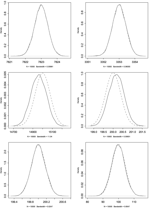
Figure 1: These plots show density estimates for the sampling distributions of $\hat{x}_{0}$, $\hat{y}_{0}$, $\hat{A}_{0}$, $\hat{S}$, $\hat{B}$, and $\hat{\theta}$, respectively, with normal densities (dashed) superimposed.

4 Model selection: how many beads are in the image

Previous authors have suggested that the number of beads in an image be determined by applying a grid search algorithm prior to fitting [Cheezum, Walker and Guilford (2001); Thompson, Larson and Webb (2002)]. As we mentioned in Section 1, any pixel with an intensity above some threshold is identified with a bead, and then some region in the vicinity of the pixel is extracted from the image and fitted. This thresholding approach may be adequate for producing initial estimates of bead locations, but thresholding prevents full automation because the threshold must be chosen by the investigator. And even a seemingly well-chosen threshold may be too large to distinguish dim beads from background noise.

Our procedure eliminates these problems by fitting first and selecting the number of beads based on those fits. In our scheme, an approximate information criterion derived from an OLS fit is used to approximate the size of the model, and then, because the candidate models are nested, likelihood ratio tests are used to select the final model. As we will show in Section 5, this approach is able to identify all of the beads, even very dim ones, automatically.

Our algorithm has a preliminary stage for estimating the number of beads and producing initial estimates of all parameters except $\theta$, and a final stage for estimating $\theta$, giving maximum likelihood estimates of the other parameters, and accurately determining the number of beads. The preliminary stage assumes zero beads initially and fits $f(x,y)=B$ to the image using OLS. Using the least squares fit at each stage, the information criterion

$$\mathit{IC}^{(k)}=n\ln\biggl{(}\frac{\mathit{RSS}}{n}\biggr{)}+p\sqrt{n}$$ (15)

is computed, where $k$ is the (assumed) number of beads, $n$ is the sample size, $\mathit{RSS}$ is the residual sum of squares, and $p$ is the number of free parameters. Note that $\mathit{IC}$ is an increasing function of $\mathit{RSS}$ and $p$, which implies that $\mathit{IC}$ rewards a better fit (smaller $\mathit{RSS}$) and penalizes more free parameters. On the next iteration, one bead is assumed, and so

$$f(x,y)=B+A_{0}\cdot\exp\biggl{(}-\frac{(x-x_{0})^{2}+(y-y_{0})^{2}}{S^{2}}\biggr{)}$$ (16)

is fit to the image, producing $\mathit{IC}^{(1)}$. Iteration continues until $\mathit{IC}^{(k)}>\mathit{IC}^{(k-1)}$, which indicates that the image contains $k-1$ beads.

Note that $\mathit{IC}$ is a nonstandard information criterion. We found that even the Bayesian Information Criteria (BIC) does not penalize additional parameters sufficiently. This can allow the initial stage of the algorithm to significantly overestimate the correct number of beads, causing much unnecessary computation during the final stage of the algorithm. Our simulations showed that replacing BIC’s $\ln(n)$ with $\sqrt{n}$ minimizes overfitting.

As the algorithm makes an initial forward sweep over possible models, the OLS parameter estimates are saved. This initial sweep stops based on the information criteria, $\mathit{IC}$. Those estimates are used to initialize the maximum likelihood estimation carried out in the final backward sweep which terminates using likelihood ratio criteria. Providing the MLE routine with good initial estimates of all parameters except $\theta$ allows the MLE to converge faster than it otherwise would.

The parameter fits and the selection criteria initially computed are then used to find the final parameter estimates and make the final model selection. The key differences are that OLS is replaced by MLE and $\mathit{IC}$ is replaced by the likelihood ratio statistic

$$G^{2}_{(\mathit{beads})}=-2\bigl{\{}\ell_{n}\bigl{(}\hat{\bolds\beta}_{\mathrm{MLE}}^{(\mathit{beads})}\bigr{)}-\ell_{n}\bigl{(}\hat{\bolds\beta}_{\mathrm{MLE}}^{(\mathit{beads}+1)}\bigr{)}\bigr{\}},$$ (17)

which should be approximately $\chi^{2}$ distributed with three degrees of freedom (because each bead is associated with three parameters: $A_{j}$, $x_{j}$, and $y_{j}$). The full algorithm is given in pseudocode below.

Algorithm 4.1 LocateBeads (pixels)

$\mathit{beads}\leftarrow 0$
$\{\hat{\bolds\beta}_{\mathrm{OLS}}^{(\mathit{beads})},\mathit{IC}^{(\mathit{beads})}\}\leftarrow\operatorname{OLS}({\mathit{pixels},\mathit{beads}})$
repeat
$\hskip 12.0pt\cases{\mathit{beads}\leftarrow\mathit{beads}+1\cr\{\hat{\bolds\beta}_{\mathrm{OLS}}^{(\mathit{beads})},\mathit{IC}^{(\mathit{beads})}\}\leftarrow\operatorname{OLS}({\mathit{pixels},\mathit{beads}})}$
until $\mathit{IC}^{(\mathit{beads})}>\mathit{IC}^{(\mathit{beads}-1)}$
$\mathit{beads}\leftarrow\mathit{beads}-1$
$\{\hat{\bolds\beta}_{\mathrm{MLE}}^{(\mathit{beads})},\ell_{n}(\hat{\bolds\beta}_{\mathrm{MLE}}^{(\mathit{beads})})\}\leftarrow\operatorname{MLE}({\mathit{pixels},\mathit{beads},\hat{\bolds\beta}_{\mathrm{OLS}}^{(\mathit{beads})})}$
repeat
$\hskip 12.0pt\cases{\mathit{beads}\leftarrow\mathit{beads}-1\cr\{\hat{\bolds\beta}_{\mathrm{MLE}}^{(\mathit{beads})},\ell_{n}(\hat{\bolds\beta}_{\mathrm{MLE}}^{(\mathit{beads})})\}\leftarrow\operatorname{MLE}({\mathit{pixels},\mathit{beads},\hat{\bolds\beta}_{\mathrm{OLS}}^{(\mathit{beads})}})\cr G^{2}_{(\mathit{beads})}\leftarrow-2\{\ell_{n}(\hat{\bolds\beta}_{\mathrm{MLE}}^{(\mathit{beads})})-\ell_{n}(\hat{\bolds\beta}_{\mathrm{MLE}}^{(\mathit{beads}+1)})\}}$
until $G^{2}_{(\mathit{beads})}>7.81=\chi^{2}_{0.95,3}$
return (${\hat{\bolds\beta}_{\mathrm{MLE}}^{(\mathit{beads}+1)}}$)

5 Simulated examples

In this section we present a series of simulated examples. We first apply our procedure to a typical image simulated from the Poisson plus Gaussian model presented above. Then we examine the robustness of our procedure by applying it in three atypical scenarios: dim beads, beads in close proximity, and beads that are not entirely contained by the image. Finally, we investigate the sensitivity of our procedure to misspecification of the instrumentation error.

First, we fit an image with fifteen roughly even-spaced fluorophores to verify that our method can handle the substantial numbers that are sometimes found in experimental data. The parameter estimates and their approximate standard errors appear in Table 2. While the time to fit such a larger example is considerable, the method works well and finds the correct number of beads without difficulties.

=200pt Parameter Truth Est error $\widehat{\mathbf{SE}}$ $x_{0}$ $23{,}566$ $0.9$ 0.422 $y_{0}$ $4852$ $0.9$ 0.423 $x_{1}$ $2522$ $-0.6$ 0.423 $y_{1}$ $18{,}672$ $0.1$ 0.421 $x_{2}$ $10{,}475$ $-0.6$ 0.424 $y_{2}$ $4858$ $-0.05$ 0.423 $x_{3}$ $16{,}643$ $-0.3$ 0.422 $y_{3}$ $19{,}505$ $0.6$ 0.423 $x_{4}$ $6842$ $0.4$ 0.423 $y_{4}$ $16{,}060$ $0.1$ 0.421 $x_{5}$ $17{,}753$ $-0.3$ 0.421 $y_{5}$ $28{,}518$ $1$ 0.423 $x_{6}$ $28{,}956$ $0.2$ 0.421 $y_{6}$ $6771$ $0.2$ 0.421 $x_{7}$ $27{,}512$ $0.3$ 0.419 $y_{7}$ $3454$ $-0.4$ 0.419 $x_{8}$ $4165$ $0.3$ 0.422 $y_{8}$ $13{,}466$ $-0.5$ 0.422 $x_{9}$ $28{,}960$ $0.4$ 0.421 $y_{9}$ $11{,}712$ $-0.5$ 0.421 $x_{10}$ $25{,}394$ $0.1$ 0.422 $y_{10}$ $28{,}468$ $-0.4$ 0.421 $x_{11}$ $29{,}112$ $0.1$ 0.423 $y_{11}$ $28{,}770$ $-0.6$ 0.422 $x_{12}$ $18{,}028$ $0$ 0.422 $y_{12}$ $21{,}796$ $0.1$ 0.422 $x_{13}$ $28{,}318$ $0.2$ 0.434 $y_{13}$ $12{,}251$ $0.2$ 0.428 $x_{14}$ $27{,}757$ $0.8$ 0.432 $y_{14}$ $11{,}937$ $0.5$ 0.426

Table 2: Localization for a Typical FIONA Image. $A=15{,}000$ for each bead, and $S=200$, $B=200$, $\theta=100$. No estimation error for $A$ was greater than $105$, and every approximate confidence interval save one covered the truth. The estimation errors for $S$, $B$, and $\theta$ were $0.1$, $-0.1$, and $1.7$, respectively, and their confidence intervals covered the true values

Figure 2 shows an image that contains a bead that is very dim ($A=400$) relative to the image’s other three beads ($A=15{,}000$). We simulated 1000 such images and applied our procedure to each. Our procedure was able to estimate the bead’s location to within a standard error of less than six nm, which, relative to the other beads, represents a tenfold decrease in resolution for a fortyfold decrease in brightness. Table 3 gives the results for this simulation study. Additionally, simulations showed our algorithm capable of consistently locating (against a background of 200) beads as dim as $A=75$, which implies a contrast ratio, that is, the ratio of the brightest pixel value and the background value, equal to 1.4 (versus 75 for a typical bead).

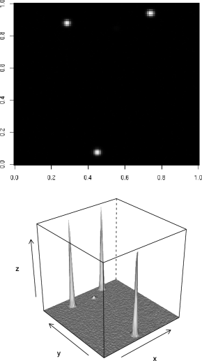
Figure 2: An image with four beads, one very dim. Our procedure locates all four beads.

Table 3: Localization of a dim bead

Parameter	Truth	Est error	Sim SE	$\widehat{\mathbf{SE}}$
$x_{0}$	$4021$	$0.03$	$0.431$	$0.422$
$y_{0}$	$5172$	$-0.13$	$0.440$	$0.422$
$A_{0}$	$15{,}000$	$69.9$	$63.339$	$49.337$
$x_{1}$	$1497$	$-0.49$	$0.430$	$0.422$
$y_{1}$	$9241$	$-0.04$	$0.428$	$0.422$
$A_{1}$	$15{,}000$	$-8$	$61.846$	$49.508$
$x_{2}$	$7920$	$-0.61$	$0.425$	$0.423$
$y_{2}$	$1807$	$0.29$	$0.405$	$0.424$
$A_{2}$	$15{,}000$	$-7.3$	$60.757$	$49.513$
$x_{3}$	$6000$	$4.69$	$5.10$	$5.03$
$y_{3}$	$8722$	$11.89$	$5.30$	$5.08$
$A_{3}$	$400$	$-8.761$	$12.377$	$11.11$
$S$	$200$	$-0.174$	$0.220$	$0.197$
$B$	$200$	$-0.194$	$0.176$	$0.174$
$\theta$	$100$	$2.575$	$4.076$	$4.25$

Figure 3 shows an image with two beads whose centers are separated by only 400 nm. We again applied our procedure to 1000 like images, each image having four beads. Our algorithm was able to distinguish the two close beads with only a slight loss of precision in the direction of the line between the beads, as is shown in Table 4.

The second image in Figure 3 shows a bead whose center is only 50 nm from the image’s edge. Our algorithm was able to localize such beads with a loss of precision in the $y$ direction that is quite acceptable and perhaps even surprisingly small given that nearly half of the bead is missing. Table 5 reports the results for a 1000-image study, where again each image had four beads.

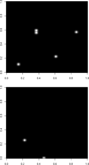
Figure 3: The upper image shows two beads in close proximity. The lower is an image with a partial bead.

Table 4: Localization of beads in close proximity

Parameter	Truth	Est error	Sim SE	$\widehat{{\mathbf{SE}}}$
$x_{0}$	$4021$	$-0.22$	$0.430$	$0.422$
$y_{0}$	$5172$	$0.45$	$0.418$	$0.421$
$A_{0}$	$15{,}000$	$22.5$	$66.827$	$54.260$
$x_{1}$	$1497$	$0.06$	$0.424$	$0.422$
$y_{1}$	$9241$	$0.36$	$0.417$	$0.423$
$A_{1}$	$15{,}000$	$30$	$62.375$	$48.019$
$x_{2}$	$7920$	$-0.21$	$0.467$	$0.445$
$y_{2}$	$1807$	$1.89$	$0.579$	$0.555$
$A_{2}$	$15{,}000$	$-17.5$	$61.06$	$48.328$
$x_{3}$	$7920$	$0.06$	$0.449$	$0.445$
$y_{3}$	$2207$	$-0.85$	$0.563$	$0.552$
$A_{3}$	$15{,}000$	$13.8$	$67.593$	$54.291$
$S$	$200$	$-0.119$	$0.190$	$0.178$
$B$	$200$	$-0.196$	$0.169$	$0.173$
$\theta$	$100$	$6.518$	$4.261$	$4.182$

Table 5: Localization of a partial bead

Parameter	Truth	Est error	Sim SE	$\widehat{\mathbf{SE}}$
$x_{0}$	$4021$	$-0.09$	$0.413$	$0.424$
$y_{0}$	$5172$	$-0.03$	$0.410$	$0.423$
$A_{0}$	$15{,}000$	$143$	$69.09$	$48.217$
$x_{1}$	$1497$	$-0.39$	$0.421$	$0.424$
$y_{1}$	$9241$	$0.39$	$0.432$	$0.424$
$A_{1}$	$15{,}000$	$143$	$69.581$	$71.17$
$x_{2}$	$7920$	$0.37$	$0.430$	$0.422$
$y_{2}$	$1807$	$0.35$	$0.417$	$0.422$
$A_{2}$	$15{,}000$	$104.4$	$64.671$	$48.416$
$x_{3}$	$6000$	$0.11$	$0.524$	$0.525$
$y_{3}$	$50$	$-0.822$	$0.924$	$0.846$
$A_{3}$	$15{,}000$	$37.2$	$62.715$	$48.738$
$S$	$200$	$-0.51$	$0.214$	$0.187$
$B$	$200$	$-0.119$	$0.169$	$0.175$
$\theta$	$100$	$0.588$	$4.243$	$4.265$

Maximum likelihood estimation is often sensitive to model misspecification, and so we investigate the performance of our procedure when the instrumentation error is not $N(0,\theta)$. The instrumentation error for each image has mean zero and variance $\theta$, but otherwise the errors are distributed rather differently. The model was simulated, but with heavy-tailed ($t_{3}$ distributed) and asymmetric (exponentially distributed) instrumentation error. More specifically, the model was simulated according to

$$Z_{i}\sim\operatorname{Poi}(f_{i})+\sqrt{\theta/3}t_{3}$$ (18)

and according to

$$Z_{i}\sim\operatorname{Poi}(f_{i})+\operatorname{Exp}\bigl{(}\sqrt{\theta}\bigr{)}-\sqrt{\theta},$$ (19)

where $\operatorname{Poi}(\lambda)$ denotes the Poisson distribution with rate $\lambda$, $t_{\nu}$ denotes the $t$ distribution with $\nu$ degrees of freedom, and $\operatorname{Exp}(\lambda)$ denotes the exponential distribution with mean $\lambda$. Tables 6 and 7 show that localization was not affected by these misspecifications. Again, 1000 images were used for each study.

Table 6: Estimation when instrumentation error is heavy-tailed

Parameter	Truth	Est error	Sim SE	$\widehat{\mathbf{SE}}$
$x_{0}$	$4021$	$-0.25$	$0.433$	$0.422$
$y_{0}$	$5172$	$-0.29$	$0.409$	$0.422$
$A_{0}$	$15{,}000$	$-18.3$	$59.564$	$47.923$
$x_{1}$	$1497$	$-0.3$	$0.437$	$0.421$
$y_{1}$	$9241$	$-0.54$	$0.425$	$0.421$
$A_{1}$	$15{,}000$	$26.9$	$65.228$	$47.658$
$x_{2}$	$7920$	$-0.19$	$0.428$	$0.422$
$y_{2}$	$1807$	$-0.13$	$0.422$	$0.422$
$A_{2}$	$15{,}000$	$33$	$58.357$	$47.671$
$x_{3}$	$6000$	$-0.6$	$0.432$	$0.421$
$y_{3}$	$8722$	$-0.1$	$0.413$	$0.422$
$A_{3}$	$15{,}000$	$-19.8$	$65.419$	$47.830$
$S$	$200$	$0.073$	$0.190$	$0.171$
$B$	$200$	$-0.017$	$0.175$	$0.173$
$\theta$	$100$	$6.435$	$9.759$	$4.191$

Table 7: Estimation when instrumentation error is asymmetric

Parameter	Truth	Est error	Sim SE	$\widehat{\mathbf{SE}}$
$x_{0}$	$4021$	$-0.26$	$0.428$	$0.420$
$y_{0}$	$5172$	$-0.75$	$0.398$	$0.421$
$A_{0}$	$15{,}000$	$5.1$	$60.595$	$47.619$
$x_{1}$	$1497$	$-0.39$	$0.410$	$0.421$
$y_{1}$	$9241$	$0.07$	$0.422$	$0.422$
$A_{1}$	$15{,}000$	$-149.7$	$62.130$	$48.146$
$x_{2}$	$7920$	$-0.17$	$0.413$	$0.421$
$y_{2}$	$1807$	$0.08$	$0.442$	$0.421$
$A_{2}$	$15{,}000$	$-68$	$57.774$	$47.940$
$x_{3}$	$6000$	$0.67$	$0.424$	$0.420$
$y_{3}$	$8722$	$0.04$	$0.420$	$0.419$
$A_{3}$	$15{,}000$	$-74$	$61.813$	$48.109$
$S$	$200$	$0.12$	$0.188$	$0.170$
$B$	$200$	$0.44$	$0.178$	$0.173$
$\theta$	$100$	$5.075$	$4.798$	$4.203$

Table 8 gives the coverage rates of our approximate 95% confidence regions for all of the previously mentioned simulation studies and for (first row) a study of 1000 typical images. The coverage rates clearly suffer a bit for all except the typical and asymmetric scenarios.

Table 8: Coverage rates of approximate 95% confidence ellipses

Scenario	Bead type	Coverage rate
Typical	typical	94.4%
	typical	95.6%
	typical	95.1%
	typical	95.4%
Dim	typical	95.6%
	typical	94.6%
	typical	95.2%
	dim	93.7%
Close	typical	95.1%
	typical	94.6%
	close	94.3%
	close	93.8%
Partial	typical	95.3%
	typical	94.5%
	typical	95.8%
	partial	93.0%
Heavy-tailed	typical	94.9%
	typical	94.3%
	typical	94.8%
	typical	93.5%
Asymmetric	typical	96.1%
	typical	95.6%
	typical	95.8%
	typical	95.2%

6 Analysis of an experimentally observed FIONA image

In this section we apply our procedure to an experimentally observed FIONA image shown in Figure 4. Table 9 shows our parameter estimates for this image.

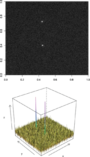
Figure 4: An experimentally observed FIONA image.

To evaluate the fit to the image, we ran numerous diagnostics to verify that the observed data originates from our random field model. Our approximate model implies that for the $i$th pixel

$$Z_{i}\stackrel{{\scriptstyle\cdot}}{{\sim}}N(f_{i},f_{i}+\theta),$$ (20)

spatially independent of the other pixels. If our model is correct, then we should have, for the $i$th error,

$$\varepsilon_{i}=\frac{Z_{i}-f_{i}}{\sqrt{f_{i}+\theta}}\stackrel{{\scriptstyle\cdot}}{{\sim}}N(0,1),$$ (21)

spatially independent of the other errors. This implies that the variogram

$$\gamma(\mathbf{h})=\tfrac{1}{2}\operatorname{Var}\{\varepsilon(\mathbf{s}+\mathbf{h})-\varepsilon(\mathbf{s})\}$$ (22)

should equal one for all locations $\mathbf{s}$ and lag (displacement) vectors $\mathbf{h}$.

=170pt Parameter Estimate $\widehat{\mathbf{SE}}$ $x_{0}$ $12{,}168.1$ $4.83$ $y_{0}$ $7570.4$ $4.79$ $A_{0}$ $269.8$ $10.5$ $x_{1}$ $12{,}296.1$ $4.71$ $y_{1}$ $16{,}509$ $4.63$ $A_{1}$ $275.7$ $10.3$ $S$ $175.7$ $3.31$ $B$ $33.4$ $0.0418$ $\theta$ $80.8$ $0.632$

Table 9: Parameter estimates for an experimentally observed FIONA image

We plot empirical (residual) variograms to determine spatial independence and use a normal probability plot to check for normality [Cressie and Hawkins (1980)]. The plots for our example image are shown in Figure 5. Except for some anomalous features in the lower tail of the probability plots, the diagnostics give a good indication that our proposed model is sound. The standardized residuals were also checked and no blatant violations of what would be expected for independent, identically distributed data were found.

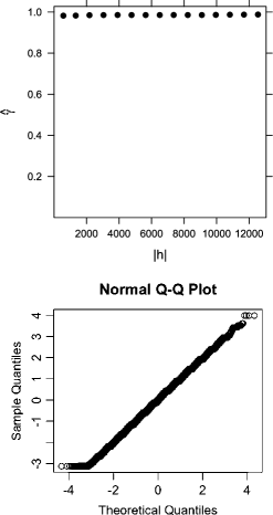
Figure 5: A variogram plot and a normal probability plot of the standardized residuals for the real FIONA image. The lags for the variogram plot are given in nanometers, and the image in question was approximately 27,000 nm on a side.

7 Conclusions

The method outlined in this paper allows for the automated analysis of FIONA images, including the ability to select the number of fluorophores in an image. By using a likelihood framework, the method also allows for standard errors to be calculated simultaneously with the estimates. The method was then verified through simulation and the analysis of collected data. We hope that this case study will serve as an example of applying traditional statistical theory to enhance the analysis of nanoscale experimental methods where algorithmic approaches have been favored.

Since this method is largely automated through model selection techniques, it can handle the analysis of “movies” by processing each frame. Since the method also returns standard errors for the locations of the fluorophores, this opens the possibility of creating tracking methods to follow dynamic specimens using not only the position data but the information on observational errors which are given.

Estimation and model selection can be done using our free C++ application, beads, which makes extensive use of the GNU Scientific Library, and fit diagnostics can be carried out using our free R software package, FIONAdiag [Galassi et al. (2008)].

References

- Bobroff (1986) Bobroff, N. (1986). Position measurement with a resolution and noise-limited instrument. Review of Scientific Instruments 57 1152–1157.
- Cheezum, Walker and Guilford (2001) Cheezum, M. K., Walker, W. F. and Guilford, W. H. (2001). Quantitative comparison of algorithms for tracking single fluorescent particles. Biophysical Journal 81 2378–2388.
- Cressie and Hawkins (1980) Cressie, N. and Hawkins, D. M. (1980). Robust estimation of the variogram: I. Math. Geol. 12 115–125. \MR0595404
- Galassi et al. (2008) Galassi, M., Davies, J., Theiler, J., Gough, B., Jungman, G., Booth, M. and Rossi, F. (2008). GNU Scientific Library Reference Manual, 1.11 ed. February.
- Kural, Balci and Selvin (2005) Kural, C., Balci, H. and Selvin, P. R. (2005). Molecular motors one at a time: Fiona to the rescue. Journal of Physics: Condensed Matter 17 S3979–S3995.
- Ravishanker and Dey (2002) Ravishanker, N. and Dey, D. K. (2002). A First Course in Linear Model Theory. Chapman & Hall/CRC, Boca Raton, FL.
- Rost (1992) Rost, F. W. D. (1992). Fluorescence Microscopy. Cambridge Univ. Press, Cambridge.
- Saxton (1997) Saxton, M. J. (1997). Single-particle tracking: The distribution of diffusion coefficients. Biophysical Journal 72 1744–1753.
- Thompson, Larson and Webb (2002) Thompson, R. E., Larson, D. R. and Webb, W. W. (2002). Precise nanometer localization analysis for individual fluorescent probes. Biophysical Journal 82 2775–2783.
- Yildiz et al. (2003) Yildiz, A., Forkey, J. N., McKinney, S. A., Ha, T., Goldman, Y. E. and Selvin, P. R. (2003). Myosin V walks hand-over-hand: Single flurophore imaging with 1.5-nm localization. Science 300 5628.