High-throughput data analysis in behavior genetics

Abstract

In recent years, a growing need has arisen in different fields for the development of computational systems for automated analysis of large amounts of data (high-throughput). Dealing with nonstandard noise structure and outliers, that could have been detected and corrected in manual analysis, must now be built into the system with the aid of robust methods. We discuss such problems and present insights and solutions in the context of behavior genetics, where data consists of a time series of locations of a mouse in a circular arena. In order to estimate the location, velocity and acceleration of the mouse, and identify stops, we use a nonstandard mix of robust and resistant methods: LOWESS and repeated running median. In addition, we argue that protection against small deviations from experimental protocols can be handled automatically using statistical methods. In our case, it is of biological interest to measure a rodent’s distance from the arena’s wall, but this measure is corrupted if the arena is not a perfect circle, as required in the protocol. The problem is addressed by estimating robustly the actual boundary of the arena and its center using a nonparametric regression quantile of the behavioral data, with the aid of a fast algorithm developed for that purpose.

[*]TGSupported in part by Israel Academy of Science Grant 915/05. , , and

1 Introduction

The open field study of behavior in animals is a subject of interest in ethology and behavior genetics, and more recently has turned out to be a working tool in drug discovery and development [Hall (1936); Bolivar, Cook and Flaherty (2000); Steele et al. (2007); Brunner, Nestlerc and Leahyc (2002)]. In such a study an animal is placed in a circular arena, with no attraction or constraints, and is free to explore it. The animals behavior is tracked to produce path data: a time series of recorded locations $(X_{i},Y_{i})$. Typical path data include tens of thousands of observations per animal with several experimental groups of animals. Quantitative summaries of the path (known as endpoints), the simplest example of which is the total distance traveled, are used by scientists to identify behavioral differences between groups.

Paths generated by rodents in an open field, while seemingly random, are structured and consist of typical patterns of behavior: progression segments separated by lingering segments [Drai, Benjamini and Golani (2000); Golani, Benjamini and Eilam (1993)]. The latter are either complete arrests or segments in time in which the rodent performs small local movements (e.g., stretching and scanning) which are captured by a sensitive tracking system.

Path data are prone to suffer from noise and outliers. During progression a tracking system might lose track of the animal, inserting (occasionally very large) outliers into the data. During lingering, and even more so during arrests, outliers are rare, but the recording noise is large relative to the actual size of the movement (the smallest value that the noise can take is 1 pixel which ranges between 0.5–2 cm). The statistical implications are that the two types of behavior require different degrees of smoothing and resistance. An additional complication is that the two interchange many times throughout a session. As a result, the statistical solution adopted needs not only to smooth the data, but also to recognize, adaptively, when there are arrests. To the best of our knowledge, no single existing smoothing technique has yet been able to fulfill this dual task. We elaborate on the sources of noise, and propose a mix of LOWESS [Cleveland (1979)] and the repeated running median [RRM; Tukey (1977)] to cope with these challenges (Section 2). Once the path has been smoothed, the quantitative summaries are computed from the smoothed path data for each animal, an approach advocated by Ramsay and Silverman (1997).

One of our experiments was conducted in 3 laboratories simultaneously, and we noticed that measures relating to distance from the wall [believed to reflect the level of anxiety of a mouse; Hall (1936); Archer (1973); Walsh and Cummins (1976); Finn, Rutledge-Gorman and Crabbe (2003)] were inconsistent across the laboratories. This is known as the replicability problem and is of deep concern in behavioral research because such experiments are conducted in many laboratories [Crabbe, Wahsten and Dudek (1999)]. A close inspection revealed that although the three arenas were supposed to be circular, one arena was slightly distorted at a level hardly noticeable to the eye, affecting the measures related to distance from the wall. Since the actual location of the wall was not available from the tracking system, the distances from the wall were computed using the planned center and radius. Clearly with such a practice, a distorted circular shape leads to wrong distance computations and consequently harms replicability.

One solution would be to build a new arena, of an exact circular shape, and rerun the experiment. However, assuring perfect circularity is difficult, and furthermore, it would not solve the possible imperfect circularity problem in other laboratories. We offer a solution utilizing the fact that mice tend to move along the boundary, and use mouse location within the arena to estimate the position of its wall by a nonparametric regression quantile [Koenker (2005)]. The rationale for the solution proposed and a technique to estimate the arena’s center are presented in Section 3.

As noted before, studies of open field behavior may have several hundreds of animals per study. Hence, any solution needs to be automatic (e.g., identification of outliers) and fast (so-called “high-throughput”). Both LOWESS and RRM meet these criteria. Our experience has shown that embedding existing nonparametric regression quantile algorithms into a high-throughput environment is difficult due to their execution time and convergence problems. As a result, we developed a fast algorithm for that purpose. The algorithm is presented in Section 3, as well as a comparison of its performance with an existing algorithm.

The motivation and characteristics of the problems addressed in the paper came from studies of mice, but the statistical and computational issues are of broader relevance. There are many other examples of studies involving automatic path tracking, including those of flies [Branson et al. (2009); Valente, Golani and Mitra (2007); Besson and Martin (2005)], pigs [Lind et al. (2005)], fish and larger marine animals [Royer and Lutcavage (2008)] and even human babies [Vitelson (2005)], to name a few. Although some of these studies address, in particular, the complications involved in the analysis of the tracked path [Lind et al. (2005); Royer and Lutcavage (2008)], most users of tracking systems are typically unaware of the consequences of the inherent noise and outliers, and the burden of providing sufficient protection is shifted onto the developers of the systems [e.g., the Ehto-Vision® tracking system; Noldus, Spink and Tegelenbosch (2001); Spink et al. (2001)].

The problem of boundary and center estimation of a circle has also a broader importance and applications in areas such as image processing [Shapiro (1978); Kim (1984)], physics [Karimaki (1991)] and the analysis of data gathered from a circular system such as an eye [Wang, Sung and Venkateswarlu (2005)], to name a few. The common assumption in these studies is that the circle is perfect and the estimation of the boundary is reduced to that of the estimation of the radius and the center, which is mostly done by least squares or maximum likelihood approaches. Efforts have been devoted to study properties of the estimator and to develop simple algorithms to solve these nonlinear problems [Chan, Elhalwagy and Thomas (2002); Zelniker and Clarkson (2006)]. Here, too, we push the current methodology forward by addressing both the estimation of the center and the boundary when the shape is only approximately circular. It is our impression that more involvement of statisticians is needed as statistical issues are ignored or handled inappropriately, for both tracking and boundary estimation problems.

2 Smoothing and identification of arrests

2.1 Noise in the tracking system

Let $(X_{i}^{0},Y_{i}^{0})$ be the actual time series of locations, and $(X_{i},Y_{i})$ the recorded time series, for $i=1,2,\ldots.$ We assume $X_{i}=X_{i}^{0}+\varepsilon_{i}$ and $Y_{i}=Y_{i}^{0}+\delta_{i}$. The velocities in the two directions are $V_{X,i}^{0}$ and $V_{Y,i}^{0}$, and the speed is $V_{i}^{0}=\sqrt{(V_{X,i}^{0})^{2}+(V_{Y,i}^{0})^{2}}$.

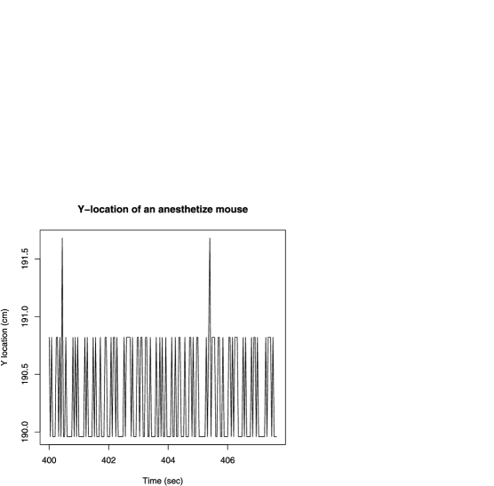
Figure 1: A typical 6 seconds of the recorded Y coordinates of an anesthetized mouse.

There are (at least) three sources for $\varepsilon,\delta$, the first two are due to the recording noise:

1. The digital recording of location in systems such as Etho-Vision® [Noldus, Spink and Tegelenbosch (2001)] together with the limited resolution implies that the arena is practically paved with “tiles” (in our case they are of size 0.5–2 cm square). In each frame the system computes the geometrical center of the mouse, and the recorded location is the center of the tile on which the geometrical center is found. Since a mouse is larger than one “tile,” recordings might vacillate between neighboring tiles. We call this the precision noise. Figure 1 illustrates vacillations between two neighboring pixels of the $Y$-location of an anesthetized mouse, over a few seconds. Naive computation of the distance traveled by this mouse during a 15 minute session gives 94 meters.

2. The erratic behavior of the tracking system when it loses track of the animal inserts outliers that may be large. To assess the extent of the problem, 30 minute sessions of mice from three strains were analyzed. We considered an observation to be an outlier if the residual between recorded and smoothed location was larger than 6 times the median of the absolute values of the residuals in the window. Slightly more than 4% of all observations were outliers.

3. Body wobble consists of movements of the animal which are not part of its whole-body progression, for example, head scanning or incipient sideways shifts of weight while running. Although they are real movements, for the purpose of studying path and velocity they are unwanted side effects and should be treated as another source of noise. Their magnitude is different for each animal type, for example, its magnitude for a turtle is larger than that for a mouse. Hence, heavier smoothing is needed for a turtle.

Precision noise and body wobble are the main sources of recording noise during lingering and arrest, while outliers are the main source of recording noise during progression.

The above examples, as well as the examples presented elsewhere in this paper, are based on a setup where the arena was circular with radius 125 cm, tracking was performed with the Ehto-Vision® tracking system [Noldus, Spink and Tegelenbosch (2001); Spink et al. (2001)] and recording was at a rate of 25 or 30 frames per second, for 30 minutes.

2.2 Smoothing locations and estimating velocities and speed

Clearly, a robust smoothing method with smooth derivatives and an automatic detection of outliers is needed. LOWESS [Cleveland (1979)] is a natural candidate for this purpose. Using a second-degree polynomial, the locations, velocities and accelerations are estimated for each direction, as a function of time. We assume that the path, at a small time window, can be approximated by

$$X_{i+t}=a_{i}+b_{i}t+c_{i}t^{2}+\varepsilon_{i},\qquad t=-h,-h+1,\ldots,0,\ldots,h.$$

The parameters $a_{i}$, $b_{i}$, $c_{i}$ are estimated using LOWESS to produce $\hat{a}_{i}$, $\hat{b}_{i}$, $\hat{c}_{i}$. In common applications of LOWESS interest lies only in the estimation of $a_{i}$ which is the expectation of $X_{i}$. Here, we are also interested in the velocity and the acceleration and we make use of all 3 estimated parameters:

$$\hat{X}_{i}=\hat{a}_{i},\qquad\hat{V}_{i}^{X}=\hat{b}_{i},\qquad\hat{A}_{i}^{X}=2\hat{c}_{i}.$$

The three quantities, in the $Y$-direction, are found similarly. We combine the two estimated series of velocities to obtain the time series of speeds: $\hat{V}_{i}=\sqrt{(\hat{V}_{i}^{X})^{2}+(\hat{V}_{i}^{Y})^{2}}$.

The data is equally spaced over time, hence, the width of the window is fixed. We choose a half-window of 10 frames (0.4 seconds), which amounts to 0.02% of the data. This is much smaller than the default of Splus or R, for example. The choice was made by the statisticians and the biologists involved who compared the smoothed path with the actual sessions on video, and checked for agreement between them. We also address this issue in the discussion.

2.3 Identifying arrests

Define an arrest as a period of time, $T$, for which $X_{t}=x$, $Y_{t}=y$ or, equivalently, $V_{t}=0$ for $t\in T$. Identifying arrests by means of zero speed is problematic, as the errors in speeds (compared to a zero speed) are all positive. Identifying arrests using LOWESS or any other averaging-based method is problematic since the smoothed locations are rarely constant due to the averaging nature of these techniques.

The running median, an old yet rarely used method, is appropriate for the purpose of identifying the time segment of an arrest. In the repeated running median [RRM; Tukey (1977)], the running median is applied iteratively, until convergence, to the sequence obtained in the previous step. Tukey proposed to perform splitting after convergence. For computational efficiency we use a variation on that in which we apply the running median 4 times, iteratively, with half-window sizes of 3, 2, 1 and 1 frames. This is done, separately, for each direction and an arrest is declared when there is no change in the smoothed locations, in both directions, for at least 0.2 seconds.

The choice of parameters was tested by comparing arrests found by the above method with arrests detected by an experienced biologist, watching videotaped sessions. A 5 minutes session of a mouse of the strain FVB was taken. The number of arrests found by the moving average, LOWESS and local polynomial were 40, 25 and 29, respectively, while our method found 97 arrests. An experienced biologist, blinded by these results, was asked to count manually the number of arrests she sees. In the course of 3 repetitions, she got 89, 96 and 102 arrests. The result of our algorithm is well in the range of arrests counted, while other methods missed many arrests. Note that even an experienced biologist may face difficulties in counting arrests (as some are very brief). The variability would likely be higher if the task was performed by several biologists. This demonstrates the need for an automated method for identifying arrests.

2.4 The combined path smoother

The dual task is smoothing location and identifying arrests, when the two modes of behavior have different characteristics and they interchange.

LOWESS is not appropriate for identifying arrests due to its averaging nature. On the other hand, neither the running median nor the RRM is appropriate for smoothing locations and obtaining velocities and accelerations, since the resulting path is too rough to represent an actual movement, and both do not provide (smooth) estimates of derivatives. Even hanning, which creates a visually more appealing smooth function, does not help here. See Section 2.5 for demonstration of these points.

We are not aware of a single method which addresses both the challenges of smoothing locations while preserving even short true bursts of arrests. We find the following combination of LOWESS and RRM to be a good solution:

1. Apply LOWESS for each direction to estimate locations and velocities.

2. Apply the variation of RRM on the raw data for each direction to identify time segments of arrests.

3. When an arrest is found, the velocities in the corresponding time segments are set to 0.

4. The smoothed locations corresponding to an arrest are linearly interpolated between the first and last frames of the arrest.

Some samples of the results obtained using the combined procedure can be viewed in Hen et al. (2004).

Biologically, arrests and local movements (e.g., head shifts) are similar, but the latter might look like progression due to the sensitivity of the tracking system. Once arrests are found, small local movements should be merged with arrests to create lingering segments. For that purpose, the maximal speed in all nonarrests segments is computed and the classification as lingering or progression is described in Drai, Benjamini and Golani (2000).

2.5 Evaluation of the combined path smoother

To evaluate the performance of the combined path smoother, we apply the method to location data of an anesthetized mouse and to simulated paths. In all cases considered the true location is known. Therefore, the properties of the smoothed paths can be compared with the properties of the actual paths.

In the case of the anesthetized mouse, noise comes from the tracking system itself, and in the simulated paths noise and outliers were built into the simulation, as described below.

We compare several smoothing approaches on location data of an anesthetized mouse (that did not move at all) which was tracked for 15 minutes. Using the recorded locations, the distance “traveled” is almost 94 m. Using the moving average, local polynomials and LOWESS, prior to computing distance, produce distances of about 8 m, 13 m and 13 meters, respectively. Using the combined method, the distance is reduced to about 3 m, much closer to the true distance which is 0. Moreover, the difference between the methods is even more pronounced when it comes to estimating the average velocity: 0.01 cm$/$s with the combined method in comparison to 0.59 cm$/$s with local polynomials—next best of the smoothing methods.

To generate simulated paths, the following steps are taken:

1. [1.]

2. A pool of velocity profiles of different lengths and shapes is generated.

3. At each step, a velocity profile is chosen at random from the pool, and the length of the arrest following the progression is chosen at random. The two are chained to the velocity profile. The total length is larger than 30,000 records.

4. The true location is computed using the time series of velocities (location at time 0 is at 0).

5. Independent $N(0,\sigma^{2})$ noise is added to the location data.

6. 4% of the nonarrests locations are chosen at random, and their locations are shifted by 5, 10 or 15 cm (with equal probability) to create outliers.

7. All locations are rounded to the nearest integer to reflect the grid structure of the data.

The above is repeated 50 times to generate replications of the paths for each set of parameters. The following properties were computed for each path:

1. [1.]

2. The actual distance traveled using the sequence obtained at stage 3 above. We denote the distance of the $i$th repetition by $\theta_{i}$.

3. The estimated distance traveled using no smoothing.

4. The estimated distance traveled after smoothing using either LOWESS, RRM or the combined method. The bandwidths used are the same as used for real tracked data. We denote the estimated distances by $\hat{\theta}_{i}$.

5. The true proportion of arrest time (0 velocity) is computed from the velocity profile and denoted by $p_{i}$.

6. The estimated proportion of arrests is computed with no smoothing and with each of the 3 smoothing methods to obtain $\hat{p}_{i}$.

We first simulated 100 paths of anesthetized mice, where the velocity profile was a time sequence of 0, and no outliers were added (since outliers occur mostly during progression). Table 1 summarizes the average and SD of distance traveled for these 100 simulated paths. The averages are of the same order of magnitude as exhibited for the tracked (real) anesthetized mouse.

Table 1: Average and SD of distance traveled over 100 simulated paths of an anesthetized mouse

	Raw	LOWESS	RRM	Combined
Ave	$113.9$	$10.1$	$24.2$	$0.96$
SD	$0.97$	$0.12$	$0.41$	$0.04$

When choosing at random a velocity profile, the 50 repetitions have a different underlying velocity profile and hence different distance travel and proportion of arrest time. We define the following MSE as our measure of performance:

$$\operatorname{MSE}(\theta)=\frac{\sum(\theta_{i}-\hat{\theta}_{i})^{2}}{50},\qquad\operatorname{MSE}(p)=\frac{\sum(p_{i}-\hat{p}_{i})^{2}}{50}.$$

Table 2 summarizes the results of the true and estimated distanced traveled as well as the MSE for the simulated paths with a velocity profile that is not identically 0.

Table 2: True (simulated) distance traveled vs. estimated distance traveled using raw data, LOWESS, RRM and the combined method

$\bolds{\sigma}$:		0.6			1	0.4
$\bolds{\bar{p}}$:		0.36	0.74	0.64	0.36	0.34
$\theta_{i}$	Ave	$732$	$299$	$416$	$712$	$745$
	SD	$92$	$69$	$83$	$84$	$82$
Raw	$\bar{\hat{\theta}}_{i}$	$967$	$609$	$704$	$1019$	$948$
	MSE	$55{,}487$	$95{,}924$	$83{,}566$	$94{,}511$	$41{,}548$
LOWESS	$\bar{\hat{\theta}}_{i}$	$737$	$311$	$426$	$721$	$749$
	MSE	$31$	$139$	$100$	$77$	$15$
RRM	$\bar{\hat{\theta}}_{i}$	$741$	$320$	$433$	$728$	$751$
	MSE	$89$	$419$	$294$	$263$	$34$
Combined	$\bar{\hat{\theta}}_{i}$	$732$	$301$	$417$	$714$	$744$
	MSE	0.07	3.1	1.6	5.5	0.4

Clearly, the combined method performs better than LOWESS and the RRM separately. Although LOWESS is second to the combined method in estimating the distance traveled, it fails to estimate the proportion of arrest time, as is evident from Table 3, which shows the proportion of arrest using each method and the corresponding MSE.

Table 3: True (simulated) proportion of arrests vs. estimated proportion using raw data, LOWESS, RRM and the combined method

$\bolds{\sigma}$:		0.6			1	0.4
$\bolds{\bar{p}}$:		0.36	0.74	0.64	0.36	0.34
Raw	$\bar{\hat{p}}_{i}$	$0.20$	$0.33$	$0.29$	$0.16$	$0.23$
	MSE	$0.03$	$0.17$	$0.12$	$0.04$	$0.01$
LOWESS	$\bar{\hat{p}}_{i}$	$0$	$0$	$0$	$0$	$0$
	MSE	$0.13$	$0.55$	$0.41$	$0.13$	$0.12$
RRM	$\bar{\hat{p}}_{i}$	$0.41$	$0.72$	$0.64$	$0.41$	$0.39$
	MSE	$0.0026$	$0.0006$	$0.0001$	$0.0027$	$0.0022$
Combined	$\bar{\hat{p}}_{i}$	$0.33$	$0.68$	$0.58$	$0.31$	$0.33$
	MSE	$0.0006$	$0.004$	$0.0027$	$0.0032$	$0.0001$

To summarize, the combined method is best in both aspects of estimating distance traveled and proportion of arrest time. Using only LOWESS or the repeated running median might be sufficient for one task but not for both.

3 Boundary and center estimation of an almost circular arena

The wall of the arena is of major importance to the mouse, affecting its behavior, in particular, the distance from the wall which is believed to be related to anxiety [Hall (1936); Archer (1973); Walsh and Cummins (1976); Finn, Rutledge-Gorman and Crabbe (2003)]. In a perfect circular arena with known radius and center, the distance is directly computed from the distance to the center. In practice, an arena might have some deviations from a perfect circle (sometimes hardly noticeable to the eye). The effect of such deviations on distance from wall, if computed under the assumed perfect circle, might be devastating. Figure 2 demonstrates the problem: the distance from wall versus the angle throughout a session is plotted for four mice: two from each strain (DBA and C57), two from each of two laboratories. In the top plots the arena was indeed a circle, and the large concentration of points near 0 was due to motion along the wall. In the middle plots the arena was of a slightly distorted circular shape. Watching the corresponding videotapes shows that these mice tended to run along the wall in the same manner as the mice in the circular arena. However, distance computations produced a wavy line since distances were computed assuming a perfect circle. To correct this, the distance between current location and actual boundary should be measured. Unfortunately, such information is not available from the tracking system.

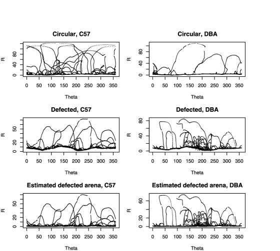
Figure 2: Distance from a perfect circular wall versus angle for two mice in the circular arena (top). The middle plots are the same but for the distorted arena. The bottom plot show the distances from the wall versus angle after boundary estimation.

One solution would be to rebuild the arena and rerun the experiment. However, assuring perfect circularity is difficult and, furthermore, it would not solve imperfect circularity in other laboratories running the experiment. We were looking for a statistical solution that would enhance the replicability of results across laboratories in future studies.

Our solution is to estimate the actual boundary from the smoothed location data of the mice. A key fact to the solution is that when a mouse progresses along the wall it typically touches it. Hence, the boundary can be inferred, indirectly, from the mouse’s extreme locations, as described below. The bottom two plots in Figure 2 show the distance from the boundary in the distorted arena, after estimation.

In our situation, using a behavioral data form within the arena to estimate its boundary is a necessity since data on actual boundary locations is not available. However, even if measurements on the boundary are available, obviously with noise, using the data from within the arena might have statistical advantages when the latter is larger in sample size (see Section 3.5).

3.1 Estimation of the boundary of the arena

Let us first assume that the location of the center of the arena is known, so let it be at the origin. Let $(\tilde{x}_{i},\tilde{y}_{i})$ be the smoothed location at time $i$, and let $R_{i}=\sqrt{\tilde{x}_{i}^{2}+\tilde{y}_{i}^{2}}$ and $\theta_{i}$ be its polar representation. In the case of a perfect circular arena with unknown radius, a natural estimate of the radius would be the maximum observed distance.

When the circle is not perfect the distance between the wall and the center is not constant, but may be assumed to change smoothly with the angle. This motivates estimating the boundary using regression of maximum distance on the angle. Some strains of mice tend to jump on the wall (in particular, during lingering, but not only), and the location of a jump is translated into locations outside the arena, hence, it is better to use some high quantile of distance, rather than the maximum. Thus, our problem can be phrased as that of a regression quantile of $R_{i}$ on $\theta_{i}$, for a high quantile, and, in particular, its nonparametric version to allow for local changes in the shape. The resultant $\hat{R}_{p}(\theta)$ for $0\leq\theta\leq 2\pi$ is the estimated boundary. The regression quantile was first introduced in Koenker and Bassett (1978), and later extended to allow for a nonparametric regression quantile [e.g., Koenker (2005)].

In principle, the quantile, $p$, might be different for different strains. Currently, the maximum or high quantile can be used and the results are almost identical. We used the 95th quantile for the results presented here, but no visual differences were noticeable when using the 99th quantile or even a higher one. An algorithm to choose the quantile can be added for a fully automated procedure, but until now there was no need for it.

The algorithm is limited to estimating only portions of the boundary where behavioral data exist. In our case, this was not a problem. However, two possible solutions are interpolation (since the boundary is almost a circle) or using the boundary estimated from another mouse that was recorded in the same arena.

3.2 Quick and easy nonparametric regression quantile

Implementation of a nonparametric regression quantile is involved and requires sophisticated algorithms [Koenker (2005)]. Two different approaches were taken by Koenker (and implemented in R in the package “quantreg”) and by Yu and Jones (1998). Using “quantreg,” we faced several difficulties: convergence problems (not solved by perturbations), slow execution time and problem with large data sets (with 30,000 locations the function did not run at all). We believe that nonstatisticians, who are the target users of the proposed approach, would be intimidated by such difficulties. We have therefore developed an alternative, fast algorithm that uses the existing LOWESS algorithm.

The input is in polar representation of all smoothed locations during progressions:

1. Divide the circle into $S$ sectors of angle $\Delta$, and let $\alpha_{s}$ be the mid-angle of each sector for $s=1,2,\ldots,S$.

2. Let $S_{s}=\{(R_{k},\theta_{k})|\alpha_{s}-\Delta/2\leq\theta_{k}\leq\alpha_{s}+\Delta/2\}$ be the collection of all polar representation of locations within a sector.

3. For $s=1,2,\ldots,S$, let $R_{s,p}$ be the $p$th quantile of $\{R_{k}|(R_{k},\theta_{k})\in S_{s}\}$.

4. Expand the data to produce an overlap at angles 0 and $2\pi$. This is done by duplicating the beginning of the series at the end, and its end at the beginning.

5. Regress $R_{s,p}$ on $\alpha_{s}$ on the expanded data, using LOWESS. Use the estimated curve between 0 and $2\pi$ as the boundary estimate.

The algorithm has two smoothing parameters. The size of a sector $\Delta$ is the first one. We used $S=720$ overlapping sectors with $\Delta=2\pi/360$. Experimentation with other numbers of sectors did not reveal significant changes. Note that the bandwidth cannot be too small (since it reflects a real boundary) or too large (since the dents would have been noticeable to the eye). We used linear LOWESS since in a small sector (1 degree amount to about 2 cm) the changes cannot be too rough. The 2nd choice of a smoothing parameter is the bandwidth of 0.15 for LOWESS. This was found in an iterative manner while checking that the resultant curve was not too rough.

The biological implications of using the algorithm may be found in Lipkind et al. (2004).

3.3 Estimations of the center of the arena

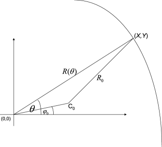
Figure 3: The relations and angles between a point on the boundary, the origin and the true center of the circle.

So far, we have assumed the center of the arena is known. Now, assume that the center $C_{0}$ is unknown, yet it is close to the origin. In this case it can be estimated using the boundary.

See Figure 3 for clarification of notation. Let $(x,y)$ be a point on the boundary, and denote its distance from $C_{0}$ by $R_{0}$. Let $(R(\theta),\theta)$ be the polar representation of $(x,y)$ and $(r_{0},\varphi_{0})$ be the polar representation of $C_{0}$. From the cosine theorem it follows that

$$R_{0}^{2}=R^{2}(\theta)+r_{0}^{2}-2R(\theta)r_{0}\cos(\theta-\varphi_{0}).$$

Hence,

$$R(\theta)=r_{0}\cos(\theta-\varphi_{0})\pm R_{0}\sqrt{1-(r_{0}/R_{0})^{2}\sin^{2}(\theta-\varphi_{0})}.$$

By assumption, $r_{0}$ is small, so, using the Taylor approximation,

$$R(\theta) = r_{0}\cos(\theta-\varphi_{0})+R_{0}+o(r_{0}/R_{0})$$

$$= R_{0}+r_{0}\cos(\varphi_{0})\cos(\theta)+r_{0}\sin(\varphi_{0})\sin(\theta)+\varepsilon.$$

In the last equation, $R_{0}$, $r_{0}$, $\varphi_{0}$ are unknown, while $R(\theta)$, $\theta$ are known. There are many points along the boundary, with polar representation: $R_{i}$, $\theta_{i}$. Using OLS, the parameters $r_{0}$, $\varphi_{0}$ may be estimated from the boundary.

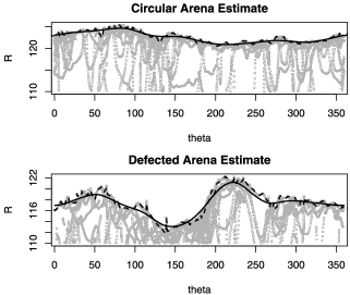
Figure 4: Estimated arena wall versus angle using our algorithm (solid) and “quantreg” (dashed). The grey points are the distances from center for smoothed locations.

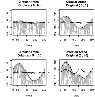
Figure 5: Estimated arena wall versus angle when the center is shifted. The grey points are as in Figure 4. The solid line is the boundary estimate using our algorithm with center estimation. The dashed line is our algorithm with no center estimation and the dotted line is the our algorithm on the original data (i.e., center not shifted).

In practice, the estimated boundary is used to estimate the center as follows:

1. [1.]

2. Use OLS to estimate $R_{0}$, $\beta_{1}$, $\beta_{2}$ in the model $R_{i}=R_{0}+\beta_{1}\cos(\theta_{i})+\beta_{2}\sin(\theta_{i})+\varepsilon_{i}$.

3. Let $\hat{r}_{0}=\sqrt{\beta_{1}^{2}+\beta_{2}^{2}}$ and $\hat{\varphi}_{0}=\cos^{-1}(\beta_{1}/\hat{r}_{0})$.

4. Let, $\hat{x}_{0}=\hat{r}_{0}\cos(\hat{\varphi}_{0})$ and $\hat{y}_{0}=\hat{r}_{0}\sin(\hat{\varphi}_{0})$.

3.4 Advantages and evaluation of the algorithms to estimate boundary and center

The proposed algorithm to estimate the boundary is simple and, consequently, it runs fast and converges well (which is especially important as part of a high-throughput environment). Depending on the size of the data, it runs 15–50 times faster than “quantreg,” and, unlike “quantreg,” we have not encountered convergence problems. Its disadvantage is the need to provide two bandwidths while “quantreg” requires only one. Cross-validation may be used to address this, but, in practice, there was no need to do so.

Figure 4 compares the two methods. The grey points are the distances of smoothed locations from $(0,0)$. The estimated boundary using our algorithm is in the solid line and using “quantreg” is in the dashed line. This was repeated for the circular and distorted arenas. Qualitatively, the results are similar; however, “quantreg” seems too rough for a physical boundary. When using other bandwidths “quantreg” did not converge.

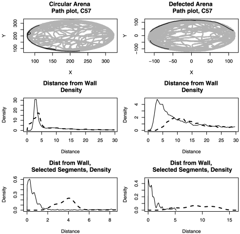
Figure 6: Typical path plot of a C57 mouse in the circular and distorted arenas. A few segments of movements along the wall were selected and marked in black. The lower 4 plots show the densities of distance from the wall for all points in the top path plot (middle) and for the selected segments (bottom) in the two arenas. The solid line is for the case where the distance is computed after boundary estimation, while the dashed line is for the case where the distance is computed assuming a perfect circle.

Figure 5 demonstrates our algorithm with and without center estimation. In the top left plot, data is from the circular arena and the presumed center is $(0,0)$. The solid line is the estimated boundary when the center was estimated as well. The dotted line is the estimated boundary with no center estimation. The difference between the two is probably because the center is not exactly at $(0,0)$. The top-right and bottom-left plots are based on the same data, but the center is shifted to the point mark at the title. The grey points are the distances from $(0,0)$ and not from the true center. The solid and dashed lines are as before. The bottom-right plot is the same but for the distorted arena.

Next we examine the density of distances from the boundary when the algorithm to estimate the boundary is being used and when it is not. The results are presented in Figure 6. For both cases, all smoothed locations within progression segments of a C57 mouse were taken. The left plots correspond to the circular arena and the right plots to the distorted one. The top plots show all the places in the arena that the mouse visited at least once. The shape of the arena is not given, but it can be deduced knowing that the mouse touches the boundary. For the circular arena, five progression segments along the boundary were chosen, and for the distorted arena three. These segments are marked in black (with some overlap between them). The middle plots are the density estimate of distances for all points belonging to progression segments. The solid line is the distance from the estimated wall, using our algorithm with center correction, while the dashed line is the density when the distances are taken from the assumed perfect circle. When the arena is indeed a circle, the two are similar, but this is not the case for the distorted arena. This effect is more dramatic when examining only the selected segments that are performed close to the wall (bottom plot). Here the effect of computing the distance from the wall, assuming a perfectly circular wall, is evident.

3.5 MSE comparison of boundary estimation

The tracking system does not provide measurements of the boundary, so we had to estimate it using behavioral data. Here, we demonstrate that even if measurements along the boundary are available, obviously with noise, using data within the arena might have statistical advantages in terms of MSE due to the different sample sizes.

We assume the center is at the origin and the constant radius is unknown, and compare estimation of the radius using boundary or behavioral data. If the arena is not a perfect circle, a nonparametric regression may be used to estimate the boundary (as described in Section 3.1).

Assume there are $n$ location measurements of the boundary and for each the distance to the origin is computed so that $R_{i}=R+\varepsilon$, where $\varepsilon$ have 0 mean and constant variance $\sigma^{2}$. Using the mean to estimate $R$, the MSE is $\sigma^{2}/n$.

Alternatively, consider the location measurements during a session, and assume that in each of the $n$ sectors there are $N$ measurements: $Z_{ij}$ for $1\leq i\leq n$ and $1\leq j\leq N$, where $Z_{ij}$ are the distances from the origin and have some distribution on a disk whose center is at the origin and its radius is $R$. The MLE of $R$ is $\max(Z_{ij})$.

Lemma 1

Assume $Z_{ij}$ are uniformly distributed on $[0,R]$ and let $\hat{R}_{1}=\max(Z_{ij})$ and $\hat{R}_{2}=(nN+1)\hat{R}_{1}/(nN)$. Then,

$$\operatorname{MSE}(\hat{R}_{1}) = R^{2}\frac{2}{(nN+1)(nN+2)},$$

$$\operatorname{MSE}(\hat{R}_{2}) = R^{2}\frac{1}{nN(nN+2)}.$$

Calculating the pdf of $\hat{R}_{1}$ is straightforward and, consequently,

$$E(\hat{R}_{1})=\frac{nN}{nN+1}R,\qquad\operatorname{var}(\hat{R}_{1})=R^{2}\frac{nN}{(nN+1)^{2}(nN+2)}.$$

The MSE of $\hat{R}_{1}$ and $\hat{R}_{2}$ follows easily.

In our setup, the mice tend to stay near the boundary for a large proportion of the time, hence, we consider a skewed distribution.

Lemma 2

Assume $Z_{ij}=RU_{ij}$ where $f(u)=(p+1)u^{p}$ for $0\leq u\leq 1$ and $p>1$. Let $\tilde{R}_{1}=\max(Z_{ij})$ and $\tilde{R}_{2}=\tilde{R}_{1}[nN(p+1)+1]/[nN(p+1)]$. Then,

$$\operatorname{MSE}(\tilde{R}_{1}) = R^{2}\frac{2}{[nN(p+1)+1][nN(p+1)+2]},$$

$$\operatorname{MSE}(\tilde{R}_{2}) = R^{2}\frac{1}{nN(p+1)[nN(p+1)+2]}.$$

Calculating the pdf of $\tilde{R}_{1}$ is straightforward and, consequently,

$$E(\tilde{R}_{1}) = R\frac{nN(p+1)}{nN(p+1)+1},$$

$$\operatorname{var}(\tilde{R}_{1}) = R^{2}\frac{nN(p+1)}{[nN(p+1)+1]^{2}[nN(p+1)+2]}.$$

The MSE of $\tilde{R}_{1}$ and $\tilde{R}_{2}$ follows easily.

The MSE based on the mean is $O(n^{-1})$, while the MSE based on the MLE (or its unbiased version) of the behavioral data is $O(n^{-2}N^{-2})$. For the case of behavioral data, using $\hat{R}_{2}$, for example, is advantageous over the boundary measurements if

$$\frac{R^{2}}{\sigma^{2}}<N(nN+2).$$

Similar comparisons are possible for the other estimators.

4 Discussion

For the dual purpose of smoothing locations and identifying arrests, we combine LOWESS and the RRM. Using LOWESS echoes the approach of Ramsay and Silverman (1997), in which the path is viewed as a smooth location function of time, and making use of its derivatives. Viewing the resultant smoothed path as a very long paragraph with no punctuation, the RRM adds the missing punctuation marks which, in turn, allows for the analysis of each sentence. The idea of adding the punctuation marks into the studied functional may be viewed as an extension of the approach of Ramsay and Silverman.

Robustness in its traditional sense is an essential component in the design of an automated high-throughput data analysis system, because it automatically protects the analysis from sources of errors that could be identified as gross errors once looked into by the human observer; alas, this observer is missing from the initial stages of the high-throughput process. A similar phenomenon happens in any data-mining operation, at the stage of ware-housing the database, preparing it for further analysis by sophisticated models and algorithms. The preparatory step is always essential and automated, and the damage that can be done at this stage is large. The use of classical robust procedures may need adaptation, and the use of shortcuts to make the extra computational effort feasible may be needed, as demonstrated by the examples given. Such an emphasis on robustness when analyzing large data sets is not usual, as robustness is associated with medium sized samples where the gain in efficiency from using robust methods may be crucial.

Estimating the boundary provides protection from deviations from the experimental design in our setup. Such deviations may happen, and when the data are processed automatically, the methods used must be robust to cope with them. This was achieved using a nonparametric regression quantile. This approach extends the common practice in image processing in which constant radius is assumed and estimated. Moreover, it turns out that our solution is more flexible than we planned: initial experimentation with the same algorithm to estimate the boundary of a squared arena performed reasonably well, indicating that extending the algorithm to take into account the possibility of corners at the boundary will yield a good general solution.

Throughout the paper we have mentioned different choices made for smoothing parameters. In all cases, the choices were made by an iterative work of biologists and statisticians, and comparison of the results to the video recordings themselves. The smoothing parameters are potentially affected by arena size, animal size, recording rate and height of ceiling, and their values should be fixated in the study protocol. Alternatively, they can be estimated via some automatic method such as cross validation based methods [e.g., Silverman (1986)], but the algorithm should be fixated as well in the protocol and be identical for all animals and groups involved. It is not clear to us whether the next step should be a development of a more sophisticated method, driven by data only, to choose the smoothing parameters or modeling the choice made by an expert as a function of the parameters defined in the study protocol (e.g., arena size, etc.). See, for example, the experience of Likhvar and Honda (2008), who demonstrated the limitations of generalized cross validation in analyzing multiple time series, where the chosen smoothing parameters occasionally missed the known curve shape.

Computation of summaries (e.g., total distance, average speed during progression) for each mouse is performed on the smoothed data, and is followed by the assessment of differences between (inbred) strains. In a single laboratory study this is done using the one-way ANOVA. Crabbe et al. executed their study in 3 laboratories, and analyzed the data using the two-way fixed ANOVA model, with strain and laboratory being the two factors. They found the interaction to be significant and their conclusion was the inability to declare replicability. In our view, the mixed model, with laboratory and interaction being random, is more appropriate [Kafkafi et al. (2005)]. The mixed model is more conservative than the fixed model, nevertheless, all 17 measures used in Kafkafi et al. showed significant differences between strains (after adjusting for multiplicity). We believe that smoothing and the ability to create homogenous classes of behavior are crucial in achieving this, and for that purpose the combination of LOWESS and the RRM plays a central rule.

We hope that publishing this paper in a statistical journal will expose more statisticians to the challenges in the field. There are open problems both in connection with the current work and more generally in the field of behavior genetics. Tracking and boundary estimation discussed here are only two of them, and are encountered as statistical problems in other fields as well.

References

- (1) Archer, J. (1973). Tests for emotionality in rats and mice: A review. Animal Behaviour 21 205–235.
- (2) Besson, M. and Martin, J.-R. (2005). Centrophobism/thigmotaxis, a new role for the mushroom bodies in Drosophila. Developmental Neurobiology 62 386–396.
- (3) Bolivar, V., Cook, M. and Flaherty, L. (2000). List of transgenic and knockout mice: Behavioral profiles. Mamm. Genome 11 260–274.
- (4) Branson, K., Robie, A. A., Bender, J., Perona, P. and Dickinson, M. H. (2009). High-throughput ethomics in large groups of Drosophila. Nature Methods 6 451–457.
- (5) Brunner, D., Nestlerc, E. and Leahyc, E. (2002). High-throughput technologies in need of high-throughput behavioral systems. Drug Discovery Today 7 S107–S112.
- (6) Chan, Y. T., Elhalwagy, Y. Z. and Thomas, S. M. (2002). Estimation of circle parameters by centroiding. J. Optim. Theory Appl. 114 363–371. \MR1920293
- (7) Cleveland, W. S. (1979). Robust locally weighted regression and smoothing scatterplots. J. Amer. Statist. Assoc. 74 829–836. \MR0556476
- (8) Crabbe, J. C., Wahlsten, D. and Dudek, B. C. (1999). Genetics of mouse behavior: Interactions with laboratory environment. Science 284 1670–1672.
- (9) Drai, D., Benjamini, Y. and Golani, I. (2000). Statistical discrimination of natural modes of motion in rat exploratory behavior. Journal of Neuroscience Methods 96 119–131.
- (10) Drai, D. and Golani, I. (2001). SEE, a tool for the visualization and analysis of rodent exploratory behavior. Neuroscience and Biobehavioral Reviews 25 409–426.
- (11) Finn, D. A., Rutledge-Gorman, M. T. and Crabbe, J. C. (2003). Genetic animal models of anxiety. Neurogenetics 4 109–135.
- (12) Hall, C. S. (1936). Emotional behavior in the rat. III. The relationship between emotionality and ambulatory activity. J. Comp. Physiol. Psychol. 22 345–352.
- (13) Hen, I., Sakov, A., Kafkafi, N., Golani, I. and Benjamini, Y. (2004). The dynamics of spatial behavior: How can robust smoothing techniques help? Journal of Neuroscience Methods 133 161–172.
- (14) Golani, I., Benjamini, Y. and Eilam, D. (1993). Stopping behavior: Constraints on exploration in rats (Rattus norvegicus). Behavioural Brain Research 53 21–33.
- (15) Kafkafi, N., Benjamini, Y., Sakov, A., Elmer, G. and Golani, I. (2005). Genotype-environment interactions in mouse behavior: A way out of the problems. Proc. Natl. Acad. Sci. USA 102 4619–4624.
- (16) Karimaki, V. (1991). Effective circle fitting for particle trajectories. Nuclear Instrumentation Methods in Physics Research 305A 187–191.
- (17) Kim, C. E. (1984). Digital disks. IEEE Transactions on Pattern Analysis and Machine Intelligence 6 372–374.
- (18) Koenker, R. (2005). Quantile Regression. Cambridge Univ. Press, Cambridge. \MR2268657
- (19) Koenker, R. and Bassett, G. S. (1978). Regression quantiles. Econometrika 46 33–50. \MR0474644
- (20) Likhvar, N. K. and Honda, Y. (2008). Choice of degree of smoothing in fitting nonparametric regression models for temparture–mortality relation in Japan based on a priori knowledge. Journal of Health Science 54 143–153.
- (21) Lind, N. M., Vinther, M., Hemmingsen, R. P. and Hansen, A. (2005). Validation of a digital video tracking system for recording pig locomotor behaviour. Journal of Neurosience Methods 143 123–132.
- (22) Lipkind, D., Sakov, A., Kafkafi, N., Elmer, G., Benjamini, Y. and Golani, I. (2004). New replicable anxiety-related measures of wall vs. center behavior of mice in the open field. Journal of Applied Physiology 97 347–359.
- (23) Noldus, L. P. J. J., Spink, A. J. and Tegelenbosch, R. A. J. (2001). EthoVision: A versatile video tracking system for automation of behavioral experiments. Behavior Research Methods, Instruments, & Computers: A Journal of the Psychonomic Society, Inc. 33 398–414.
- (24) Ramsay, J. and Silverman, B. (1997). Functional Data Analysis. Springer, New York. \MR2168993
- (25) Royer, F. and Lutcavage, M. (2008). Filtering and interpreting location errors in Satellite telemetry of marine animals. Journal of Experimental Marine Biology and Ecology 359 1–10.
- (26) Shapiro, S. D. (1978). Properties of transforms for the detection of curves in noisy pictures. Computer Vision Graphics and Image Processing 8 129–143.
- (27) Silverman, B. (1986). Density Estimation for Statistics and Data Analysis. Chapman & Hall, London. \MR0848134
- (28) Spink, A. J., Tegelenbosch, R. A. J., Buma, M. O. S. and Noldus, L. P. J. J. (2001). The EthoVision video tracking system—A tool for behavioral phenotyping of transgenic mice. Physiology & Behavior 73 731–734.
- (29) Steele, A. D., Jackson, W. S., King, O. D. and Lindquist, S. (2007). The power of automated high-resolution behavior analysis revealed by its application to mouse models of Huntington’s and prion diseases. Proc. Natl. Acad. Sci. 104 1983–1988.
- (30) Tukey, J. W. (1977). Exploratory Data Analysis. Addison-Wesley, Reading, MA.
- (31) Valente, D., Golani, I. and Mitra, P. P. (2007). Analysis of the trajectory of Drosophila melanogaster in a circular open field arena. PLoS ONE 2(10) e:1083 DOI:10.1371/journal.pone.0001083.
- (32) Vitelson, H. (2005). Spatial behavior of pre-walking infants: Patterns of locomotion in a novel environment. Ph.D. thesis, Tel Aviv Univ.
- (33) Walsh, R. N. and Cummins, R. A. (1976). The open-field test: A critical review. Psychological Bulletin 83 482–504.
- (34) Wang, H. G., Sung, E. and Venkateswarlu, R. (2005). Estimating the eye gaze from one eye. Computer Vision and Image Understanding 98 83–103.
- (35) Yu, K. and Jones, M. C. (1998). Local linear quantile regression. J. Amer. Statist. Assoc. 93 228–237. \MR1614628
- (36) Zelniker, E. and Clarkson, I. V. L. (2006). A statistical analysis of the Delogne–Kasa method for fitting circle. Digital Signal Processing 16 498–522.