One-Shot Multiparty State Merging

Abstract

We present a protocol for performing state merging when multiple parties share a single copy of a mixed state, and analyze the entanglement cost in terms of min- and max-entropies. Our protocol allows for interpolation between corner points of the rate region without the need for time-sharing, a primitive which is not available in the one-shot setting. We also compare our protocol to the more naive strategy of repeatedly applying a single-party merging protocol one party at a time, by performing a detailed analysis of the rates required to merge variants of the embezzling states. Finally, we analyze a variation of multiparty merging, which we call split-transfer, by considering two receivers and many additional helpers sharing a mixed state. We give a protocol for performing a split-transfer and apply it to the problem of assisted entanglement distillation.

I Introduction

An important part of quantum information theory is concerned with the design and analysis of quantum communication protocols. The subject has flourished over the past two decades, with early discoveries like teleportation teleportation and superdense coding superdense laying the groundwork for a series of major advances over the last five years. (See, for example, SVW ; Merge ; Hayden001 ; DW ; Yard01 ; Yard02 ; zero ; hasting .) Another early result, Schumacher compression Schumacher , studies the amount of quantum communication required to transmit to another location a sequence of quantum states $|\psi^{A}_{1}\rangle|\psi^{A}_{2}\rangle|\psi^{A}_{3}\rangle\ldots$ emitted by a statistical source. If we assume the states coming from the source are independent and identically distributed (i.e an i.i.d source), we get the quantum analogue of Shannon compression, and the optimal rate of compression is given by the von Neumann entropy $S(\rho)$ of the density matrix $\rho=\sum_{j}p_{j}\psi_{j}$ associated with the source Schumacher . This gives an informational meaning to the von Neumann entropy, whose original definition was motivated by the desire to extend the Gibbs entropy, a thermodynamical concept, to the quantum setting. Schumacher compression is often used in more complex protocols as a preliminary preprocessing step.

Other information theoretic quantities, such as the conditional von Neumann entropy $S(A|B)_{\psi}$ Negative and the conditional mutual information $I(A:B|R)_{\psi}$ Yard01 , were only more recently given meaning SW-nature ; Merge ; Yard01 . If we consider an i.i.d. source $S$ emitting an unknown sequence of states $|\psi^{AB}_{1}\rangle|\psi^{AB}_{2}\rangle\ldots|\psi^{AB}_{n}\rangle$, distributed to two spatially separated parties $A$ (Alice) and $B$ (Bob), an interpretation of $S(A|B)_{\psi}$ can be obtained SW-nature ; Merge as the optimal rate at which pure entanglement needs to be consumed in order to transfer the entire sequence to Bob’s location. Whenever $S(A|B)_{\psi}$ is negative, it is understood that entanglement is gained instead of consumed and that the transfer can be accomplished using only local operations and classical communication (LOCC). The first protocol Merge ; SW-nature for achieving this task, also known as state merging, was based on a random measurement strategy, a popular approach when designing quantum communication protocols. Examples of other tasks that can be achieved using this approach are distributed compression Hayden002 and assisted distillation dfm . In assisted distillation, $m$ helpers $C_{1},C_{2},\ldots,C_{m}$ and two recipients $A$ and $B$ share a multipartite pure state $\psi^{C_{1}C_{2}\ldots C_{m}AB}$, and the objective is to extract an optimal amount of pure entanglement between $A$ and $B$ by using LOCC operations and classical information broadcasted by the $m$ helpers $C_{1},C_{2},\ldots,C_{m}$.

Both distributed compression and assisted distillation involve multiple parties (i.e more than two) sharing a multipartite state $\psi$. In the case of distributed compression, we can use the state merging primitive to perform compression at an optimal rate by transferring each sender’s share one at a time Merge . This strategy will work for any rate which is a corner point of the boundary of the rate region associated with distributed compression. To achieve compression at rates which are not corner points, however, we need to use a time-sharing strategy as the decoding operation performed by the receiver can only recover the shares one at a time. One contribution of this paper is to present a protocol for the more general task of multiparty state merging which will eliminate the need for time-sharing. That is, we consider $m$ senders $C_{1},C_{2},\ldots,C_{m}$ and a decoder $B$ sharing a multipartite mixed state $\psi^{C_{1}C_{2}\ldots C_{m}B}$, potentially with additional entanglement in the form of EPR pairs (ebits) distributed between the decoder and each of the $m$ senders. Given many copies of the input state $\psi^{C_{1}C_{2}\ldots C_{m}B}$, the task is to transfer the shares $C_{1},C_{2},\ldots,C_{m}$ to the receiver $B$ with high fidelity using only LOCC operations.

If only a single copy of the state $\psi^{C_{1}C_{2}\ldots C_{m}B}$ is available to the parties, we can use our protocol to achieve merging within an error tolerance $\epsilon$ if we distribute enough initial entanglement between each of the senders and the receiver. In this regime, a more naive strategy consisting of repeatedly applying a one-shot state merging protocol Berta on one sender at a time will generally require more initial entanglement to perform the state transfer than does our protocol. In addition, this strategy only yields a handful of achievable combinations of entanglement costs and does not permit interpolating between them. A full characterization of the entanglement cost in the one-shot regime when $m=1$ was performed by Berta using smooth min- and max-entropies. By applying the random measurement strategy of Merge and by using the min- and max-entropy formalism of Renner02 , we generalize some of the results of Berta to the multipartite case ($m\geq 2$). This work complements other recent attempts to study quantum information theory in the one-shot setting Renner01 ; Berta02 ; Datta1 ; Datta ; Renes .

To perform assisted distillation in the context of multiple parties, we introduce a second decoder, whom we label $A$ (Alice), and consider a variation of multiparty merging. Given a partition of the helpers $C_{1},C_{2}\ldots,C_{m}$ into a set ${\cal T}$ and its complement $\overline{{\cal T}}:=\{C_{1}C_{2}\ldots C_{m}\}\backslash{\cal T}$, we want to transfer the shares ${\cal T}$ and ${\overline{\cal T}}$ to the locations of the decoders $A$ and $B$ respectively. We call this task a split-transfer of the state $\psi^{C_{1}C_{2}\ldots C_{m}B}$. A protocol for performing a split-transfer can be obtained by using the random measurement strategy on $C_{1},C_{2},\ldots,C_{m}$, followed by appropriate decodings $U_{A}$ and $V_{B}$ by the decoders $A$ and $B$. The optimal achievable rate for assisted distillation was found in Merge by using a recursive argument. By using a split-transfer protocol, we give a simpler demonstration which does not rely on a recursive argument.

Structure of the paper: In Section II, we introduce the definition for multiparty merging of a state $\psi^{C_{1}C_{2}\ldots C_{m}BR}$ and review the known results for the i.i.d setting. In Section III, we formulate a condition that a set of instruments performed by the senders $C_{1},C_{2},\ldots,C_{m}$ must satisfy in order to accomplish merging within a fixed error tolerance. In Section IV, we consider random measurements performed by the senders $C_{1},C_{2},\ldots,C_{m}$ and prove an upper bound to the quantum error when a single copy of the input state is available. We analyze the asymptotic setting in Section V, recovering the main theorem of Section II without the need for time-sharing. In Section VI, we reformulate the bounds obtained in Section III in terms of min-entropies and give necessary and sufficient conditions for merging in the one-shot regime. SectionVII is devoted to analyzing the rates achievable for variants of the embezzling states, comparing our protocol to a strategy of merging the shares one at a time. We introduce a split-transfer of the state $\psi^{C_{1}C_{2}\ldots C_{m}B}$ in Section VIII and show the existence of a protocol for performing this task. We use this protocol to recover the optimal distillation rate for the problem of assisted distillation. Appendices, containing relevant folklore material, appear at the end.

Notation: In this paper, we restrict our attention to finite dimensional Hilbert spaces. Quantum systems under consideration will be denoted $A,B,\ldots,$ and are freely associated with their Hilbert spaces, whose (finite) dimensions are denoted $d_{A},d_{B}$, etc… If $A$ and $B$ are two Hilbert spaces, we write $AB\equiv A\otimes B$ for their tensor product and write $A^{n}$ for the tensor product $\bigotimes_{i=1}^{n}A$. If we have $m$ Hilbert spaces $A_{1},A_{2},\ldots,A_{m}$, we write $A_{M}$ for the tensor product $\bigotimes^{m}_{i=1}A_{i}$. An ancilla augmenting the system $A_{i}$ is denoted as $A^{0}_{i}$. We write $A^{0}_{M}$ for the tensor product $\bigotimes^{m}_{i=1}A^{0}_{i}$ of $m$ ancillas $A^{0}_{1},A^{0}_{2},\ldots,A^{0}_{m}$. The maximally entangled state $\frac{1}{\sqrt{K_{i}}}\sum_{k=1}^{K_{i}}|k\rangle|k\rangle$ of Schmidt rank $K_{i}$ is denoted as $|\Phi^{K_{i}}\rangle$. We write $\Phi^{K}$ for the density operator $|\Phi^{K_{1}}\rangle\langle\Phi^{K_{1}}|\otimes|\Phi^{K_{2}}\rangle\langle\Phi^{K_{2}}|\otimes\ldots\otimes|\Phi^{K_{m}}\rangle\langle\Phi^{K_{m}}|$. The space of linear operators acting on the Hilbert space $A$ is denoted by ${\cal L}(A)$. The identity operator acting on $A$ is denoted by $I^{A}$. The symbol $\mathrm{id}_{A}$ denotes the identity map acting on ${\cal L}(A)$. Unless otherwise stated, a ”state” can be either pure or mixed. The symbol for such a state (such as $\psi$ and $\rho$) also denotes its density operator. The density operator $|\psi\rangle\langle\psi|$ of a pure state will frequently be written as $\psi$. We denote by $\tau_{A}$ the maximally mixed state of dimension $d_{A}$. We write $S(A)_{\psi}=-\mathrm{Tr}(\psi^{A}\log\psi^{A})$ to denote the von Neumann entropy of a density matrix $\psi^{A}$ for the system $A$. The function $F(\rho,\sigma):=\mathrm{Tr}\sqrt{\rho^{1/2}\sigma\rho^{1/2}}$ is the fidelity uhlmann:fid between the two states $\rho$ and $\sigma$. The trace norm of an operator, $\|X\|_{1}$ is defined to be $\mathrm{Tr}|X|=\mathrm{Tr}\sqrt{X^{{\dagger}}X}$. We will use the terms ”receiver” and ”decoder” interchangeably throughout the following sections.

II Definitions and Main Result

For a bipartite state $\rho^{AB}$, the operation known as quantum state merging can be viewed in two different ways. The original formulation of the problem Merge was in terms of a statistical source emitting (unknown) states $|\psi^{AB}_{1}\rangle,|\psi^{AB}_{2}\rangle,\ldots,$ with average density operator $\rho^{AB}$ assumed to be known by the parties. The objective was then to transfer the entire sequence to the location of the decoder (Bob) using as little quantum communication as possible. An equivalent view of the problem is to consider a purification $\psi^{ABR}$ of the density matrix $\rho^{AB}$, and regard the process of merging as that of transferring all the correlations between Alice’s share and the purification system $R$ to the location of the decoder $B$. This means decoupling Alice’s system from the reference $R$, while leaving the state $\psi^{R}$ intact (up to some arbitrarily small perturbation) in the process. The receiver will hold a purification $\phi^{BR}$ of the system $R$, and since all purifications are equivalent up to an isometry on the purification system, he can recover the original state $\psi^{ABR}$ by applying an appropriate isometry to $\phi^{BR}$. Additional entanglement between Alice and Bob might be distilled in the process.

To analyze the multipartite scenario, where $m$ senders and a decoder/receiver share a state $\psi^{C_{1}C_{2}\ldots C_{m}BR}$, with purifying system $R$, we adopt the second view and look at the transformations that can be performed by the senders on their shares to allow the receiver to recover the purified state $\psi^{C_{1}C_{2}\ldots C_{m}BR}$ with high fidelity. The resources at their disposal will be pure entanglement, in the form of maximally entangled states shared between each of the senders $C_{1},C_{2},\ldots,C_{m}$ and the receiver Bob, and noiseless classical channels, which will be used to transmit measurement outcomes to the receiver. Any transformation applied by the senders will need to decouple the reference $R$ from the senders’ shares $C_{1},C_{2},\ldots,C_{m}$ and leave the reference unchanged. Otherwise, the receiver might hold a purification that cannot be taken, by means of an isometry, to the original state. If each of the senders $C_{1},C_{2},\ldots,C_{m}$ perform an incomplete measurement, described by Kraus operators $P_{i}$ mapping $C_{i}$ to a subspace $C^{1}_{i}$, we would want each outcome state $\psi^{C^{1}_{1}C^{1}_{2}\ldots C^{1}_{m}R}_{J}$ to have a product form

$$\psi^{C^{1}_{1}C^{1}_{2}\ldots C^{1}_{m}R}_{J}\approx\psi^{C^{1}_{1}C^{1}_{2}\ldots C^{1}_{m}}_{J}\otimes\psi^{R},$$ (1)

where $J=(j_{1},j_{2},\ldots,j_{m})$ are the measurement outcomes. The states $\{\psi^{C^{1}_{1}C^{1}_{2}\ldots C^{1}_{m}}_{J}\}$ could be entangled and/or contain classical correlations between some of the subsystems $C^{1}_{1},C^{1}_{2},\ldots,C^{1}_{m}$. In this paper, we will primarily be concerned with extracting pure bipartite entanglement, in the form of maximally entangled states $\frac{1}{\sqrt{K}}\sum^{K}_{i=1}|k\rangle|k\rangle$ shared between the senders and the decoder, and thus, we will further impose that the operations applied by the senders destroy all correlations existing with the other senders’ shares. That is, we want

$$\psi^{C^{1}_{1}C^{1}_{2}\ldots C^{1}_{m}R}_{J}\approx\tau^{C^{1}_{1}}\otimes\tau^{C^{1}_{2}}\otimes\ldots\otimes\tau^{C^{1}_{m}}\otimes\psi^{R},$$ (2)

where $\tau^{C^{1}_{i}}$ is the maximally mixed state of dimension $L_{i}$ on the subspace $C^{1}_{i}$. With this assumption in mind, we can give a definition of a multiparty state merging for a state $\psi^{C_{1}C_{2}\ldots C_{m}BR}$.

Figure 1: Picture of the initial and final steps of a multiparty state merging protocol.

Let $\Lambda^{m}_{\rightarrow}:C_{M}C^{0}_{M}\otimes BB^{0}_{M}\rightarrow C^{1}_{M}\otimes B^{1}_{M}BB_{M}$ be an LOCC quantum operation performed by the senders $C_{1},C_{2},\ldots,C_{m}$ and the decoder $B$. Initially, each sender $C_{i}$ is given an ancilla $C^{0}_{i}$. The receiver also has ancillas $B^{0}_{M}:=B^{0}_{1}B^{0}_{2}\ldots B^{0}_{m}$, with $d_{B^{0}_{i}}=d_{C^{0}_{i}}$, and $B^{1}_{M}:=B^{1}_{1}B^{1}_{2}\ldots B^{1}_{m}$ with $d_{B^{1}_{i}}=d_{C^{1}_{i}}$. Before the map $\Lambda^{m}_{\rightarrow}$ is applied, the systems $C^{0}_{M}$ and $B^{0}_{M}$ will hold maximally entangled states $\Phi^{K_{1}}\otimes\Phi^{K_{2}}\otimes\ldots\otimes\Phi^{K_{m}}$, where $\Phi^{K_{i}}$ has Schmidt rank $K_{i}=d_{C^{0}_{i}}$ and is shared between the sender $C_{i}$ and the receiver $B$. After the map $\Lambda^{m}_{\rightarrow}$ is applied, the senders share a subsystem $C^{1}_{M}:=C^{1}_{1}C^{1}_{2}\ldots C^{1}_{m}$ of $C_{M}$, and the receiver holds three systems: $B$, $B^{1}_{M}$ and $B_{M}$, with $B_{M}$ being an ancillary system of dimension of the same size as the system $C_{M}$.

This operation will implement merging, as illustrated in Figure 1, if the output state of the map $\mathrm{id}_{R}\otimes\Lambda^{m}_{\rightarrow}$ is approximately a tensor product of the initial state $\psi^{C_{1}C_{2}\ldots C_{m}BR}$ and maximally entangled states $\Phi^{L}:=\Phi^{L_{1}}\otimes\Phi^{L_{2}}\otimes\ldots\otimes\Phi^{L_{m}}$ shared between the senders and the decoder. Each $\Phi^{L_{i}}$ is a maximally entangled state of Schmidt rank $L_{i}$ on the tensor space $C^{1}_{i}B^{1}_{i}$. More formally, we have

Definition 1 ($m$-Party State Merging)

Let $\Lambda^{m}_{\rightarrow}$ be defined as in the previous paragraphs. We say that $\Lambda^{m}_{\rightarrow}$ is an $m$-party state merging protocol for the state $\psi^{C_{1}C_{2}\ldots C_{m}BR}$ with error $\epsilon$ and entanglement cost $\overrightarrow{E}:=(\log K_{1}-\log L_{1},\log K_{2}-\log L_{2},\ldots,\log K_{m}-\log L_{m})$ if

$$\biggl{\|}(\mathrm{id}_{R}\otimes\Lambda^{m}_{\rightarrow})(\psi^{C_{1}C_{2}\ldots C_{m}BR}\otimes\Phi^{K})-\psi^{B_{M}BR}\otimes\Phi^{L}\biggr{\|}_{1}\leq\epsilon,$$ (3)

where the state $\psi^{B_{M}BR}$ corresponds to the initial state $\psi^{C_{1}C_{2}\ldots C_{m}BR}$ with the system $B_{M}$ substituted for $C_{M}$. If we are given $n$ copies of the same state, $\psi=(\sigma)^{\otimes n}$, the entanglement rate $\overrightarrow{R}(\sigma)$ is defined as $\overrightarrow{R}(\sigma):=\frac{1}{n}\overrightarrow{E}(\psi)$.

Before stating the main theorem, we need to define what it means for a rate-tuple $\overrightarrow{R}$ to be achievable for multiparty merging using LOCC operations.

Definition 2 (The Rate Region)

We say that the rate-tuple $\overrightarrow{R}:=(R_{1},R_{2},\ldots,R_{m})$ is achievable for multiparty merging of the state $\psi^{C_{1}C_{2}\ldots C_{m}B}$ if, for all $\epsilon>0$, we can find an $N(\epsilon)$ such that for every $n\geq N(\epsilon)$ there exists an $m$-party state merging protocol $\Lambda^{m}_{\rightarrow}$ acting on $\psi^{\otimes n}\otimes\Phi^{K^{n}}$, with error $\epsilon$ and entanglement rate $\overrightarrow{R_{n}}:=\frac{1}{n}(\log K^{n}_{1}-\log L^{n}_{1},\log K^{n}_{2}-\log L^{n}_{2},\ldots,\log K^{n}_{m}-\log L^{n}_{m})$ approaching $\overrightarrow{R}$. We call the closure of the set of achievable rate-tuples the rate region.

Suppose $m$ systems $C_{1},C_{2},\ldots,C_{m}$ in the state $\psi^{C_{1}C_{2}\ldots C_{m}R}$, where $R$ is a purifying system, are distributed to $m$ senders, spatially separated from each other. To recover the purified state $\psi^{C_{1}C_{2}\ldots C_{m}R}$ at the receiver’s end, a task called distributed compression, the senders need an enough supply of initial entanglement. It was shown in Merge that the rate region associated with distributed compression is characterized by the inequalities

$$\sum_{i\in{\cal T}}R_{i}\geq S({\cal T}|\overline{{\cal T}})_{\psi}\phantom{==}\quad\text{for all nonempty sets }{\cal T}\subseteq\{1,2,\ldots,m\}.$$ (4)

Here, the symbol ${\cal T}$ also denotes the tensor product space ${\cal T}:=\bigotimes_{i\in{\cal T}}C_{i}$ associated with the set ${\cal T}$. The set $\overline{{\cal T}}$ is defined as $\{1,2,\ldots,m\}\backslash{\cal T}$ and the tensor product space $\overline{{\cal T}}$ as $\bigotimes_{i\in{\overline{\cal T}}}C_{i}$. If a rate-tuple $(R_{1},R_{2},\ldots,R_{m})$ is achievable for distributed compression and some of the rates $R_{i}$ are negative, then the senders $C_{i}$ will be able to transfer their shares to the receiver using only LOCC operations, and furthermore, they will gain a potential for future communication in the form of maximally entangled states. Allowing the receiver to have side information $B$ as well, leads to a similar set of equations describing the rate region associated with the task of multiparty state merging.

Theorem 3 ($m$-Party Quantum State Merging Merge )

Let $\psi^{C_{1}C_{2}\ldots C_{m}BR}$ be a pure state shared between $m$ senders $C_{1},C_{2},\ldots,C_{m}$ and a receiver Bob, with purifying system $R$. Then, the rate $\overrightarrow{R}:=(R_{1},R_{2},\ldots,R_{m})$ is achievable for multiparty merging iff the inequality

$$\sum_{i\in{\cal T}}R_{i}\geq S({\cal T}|\overline{{\cal T}}B)_{\psi}$$ (5)

holds for all non empty subsets ${\cal T}\subseteq\{1,2,...,m\}$.

The theorem was proved in Merge by showing that the corner points of the region are achievable and then using time-sharing to interpolate between them. In addition to recovering the result without time-sharing, we will extend it to the one-shot setting. Time-sharing, which consists of partitioning a large supply of states and applying different protocols to each subset, is impossible if only a single copy of a state is available. Instead, we will construct a single protocol which merges all shares at once.

III Conditions for Merging Many Parties

Let’s try to construct an LOCC operation $\Lambda^{m}_{\rightarrow}:C_{M}C^{0}_{M}\otimes BB^{0}_{M}\rightarrow C^{1}_{M}\otimes B^{1}_{M}BB_{M}$ that when applied to the state $\psi^{C_{1}C_{2}\ldots C_{m}B}\otimes\Phi^{K}$ will achieve merging, and destroy all existing correlations between the senders’ shares $C_{1},C_{2},\ldots,C_{m}$ at the same time. It can be seen as a three step process:

• First, each sender $C_{i}$ applies a quantum instrument ${{\cal I}_{i}}:=\{{\cal E}^{i}_{j}\}^{X}_{j=1}$ to his share of the state $\psi^{C_{1}C_{2}\ldots C_{m}BR}\otimes\Phi^{K}$. This will yield both quantum and classical outputs. Each operator ${\cal E}^{i}_{j}$ for the instrument ${\cal I}_{i}$ is completely positive, and maps the space $C_{i}C^{0}_{i}$ to the subspace $C^{1}_{i}$.

• Secondly, the senders $C_{1},C_{2},\ldots,C_{m}$ send their classical outputs $J:=(j_{1},j_{2},\ldots,j_{m})$ to the decoder $B$.

• Finally, the decoder will use his side information $\psi^{B}$, his share of the maximally entangled states $\{\Phi^{K_{i}}\}$, and the classical information $J$ to perform a decoding operation ${\cal D}_{J}:BB^{0}_{M}\rightarrow B^{1}_{M}BB_{M}$ (i.e a trace-preserving completely positive map (TP-CPM)) and recover the state $\psi^{C_{1}C_{2}\ldots C_{m}BR}\otimes\Phi^{L}$.

The state of the systems $C^{1}_{M}B^{0}_{M}BRX$ after steps 1 and 2 are performed can be written as:

$$\begin{split}\psi^{C^{1}_{M}B^{0}_{M}BRX}&:=\sum_{J:=j_{1}j_{2}\ldots j_{m}}[(\mathrm{id}^{B^{0}_{M}BR}\otimes{\cal E}_{J})(\psi^{C_{1}C_{2}\ldots C_{m}BR}\otimes\Phi^{K})]^{C^{1}_{M}B^{0}_{M}BR}\otimes|J\rangle\langle J|^{X}\\ &=\sum_{J}p_{J}\psi_{J}^{C^{1}_{M}B^{0}_{M}BR}\otimes|J\rangle\langle J|^{X},\\ \end{split}$$ (6)

where ${\cal E}_{J}:={{\cal E}}^{1}_{j_{1}}\otimes{{\cal E}}^{2}_{j_{2}}\otimes\ldots\otimes{{\cal E}}^{m}_{j_{m}}$ and $\psi_{J}^{C^{1}_{M}B^{0}_{M}BR}$ is the normalized state given by $(\mathrm{id}^{B^{0}_{M}BR}\otimes{\cal E}_{J})(\psi^{C_{1}C_{2}\ldots C_{m}BR}\otimes\Phi^{K})$. The system $X$ is an ancillary system held by the receiver which contains the classical outputs of the instruments ${\cal I}_{1},{\cal I}_{2},\ldots,{\cal I}_{m}$. If we restrict the operators ${\cal E}^{i}_{j}$ to consist of only one Kraus operator (i.e ${\cal E}^{i}_{j}(\rho)=A^{i}_{j}\rho(A^{i}_{j})^{{\dagger}}$ for all $i,j$) and to satisfy $\sum_{j}(A^{i}_{j})^{{\dagger}}A^{i}_{j}=I^{C_{i}}$, the outcome states $\{\psi^{C^{1}_{M}B^{0}_{M}BR}_{J}\}$ are pure and are the result of performing $m$ incomplete measurements, one for each sender $C_{i}$.

After the senders have finished performing their instruments, we would ideally like for the state $\psi^{C^{1}_{M}R}_{J}$ to be in the product form

$$\begin{split}\psi_{J}^{C^{1}_{M}R}&=\tau^{C^{1}_{1}}\otimes\tau^{C^{1}_{2}}\otimes\ldots\otimes\tau^{C^{1}_{m}}\otimes\psi^{R},\\ &=\tau^{C^{1}_{M}}\otimes\psi^{R},\\ \end{split}$$ (7)

where $\tau_{C^{1}_{i}}$ is the maximally mixed state of dimension $L_{i}=d_{C^{1}_{i}}$ on the space $C^{1}_{i}$. Suppose, for the moment, that this property is satisfied for all $\{\psi_{J}^{C^{1}_{M}R}\}$. Then, the state $\psi_{J}^{C^{1}_{M}B^{0}_{M}BR}$ purifies $\tau^{C^{1}_{M}}\otimes\psi^{R}$, with purification systems $B^{0}_{M}B$. Another purification of $\tau^{C^{1}_{M}}\otimes\psi^{R}$ is also given by $\Phi^{L}\otimes\psi^{B_{M}BR}$, where the state $\psi^{B_{M}BR}$ corresponds to the original state $\psi^{C_{1}C_{2}\ldots C_{m}BR}$ with the system $B_{M}$ substituted for $C_{M}$. It follows from the Schmidt decomposition that these two purifications are related by an isometry $U_{J}:B^{0}_{M}B\rightarrow B^{1}_{M}BB_{M}$ on Bob’s side such that

$$\begin{split}(I^{C^{1}_{M}R}\otimes U_{J})\psi_{J}^{C^{1}_{M}B^{0}_{M}BR}(I^{C^{1}_{M}R}\otimes U_{J})^{{\dagger}}&=\Phi^{L_{1}}\otimes\Phi^{L_{2}}\otimes\ldots\otimes\Phi^{L_{m}}\otimes\psi^{B_{M}BR},\\ &=\Phi^{L}\otimes\psi^{B_{M}BR}.\\ \end{split}$$ (8)

Hence, if the senders can perfectly decouple their systems $C_{M}C^{0}_{M}$ from the reference, their ”$R$-entanglement” will be transferred to Bob’s location. Furthermore, by applying $U_{J}$, the receiver will recover the original state and distill some pure bipartite entanglement.

The previous scenario was ideal, and in general, will not be feasible for most states $\psi^{C_{1}C_{2}\ldots C_{m}BR}$. Hence, we relax our decoupling requirement and accept that the measurements performed by the senders will perturb the reference $\psi^{R}$ up to some tolerable amount, and that a small dose of correlations between the senders’ shares might still be present. In more formal terms, we have

Proposition 4 (Compare to Proposition 4 of Merge )

Let $\psi_{J}^{C^{1}_{M}B^{0}_{M}BR}$ be defined as in eq. (6), with reduced density matrix $\psi_{J}^{C^{1}_{M}R}$. Define the following quantity:

$$Q_{{\cal I}}(\psi^{C_{1}C_{2}\ldots C_{m}BR}\otimes\Phi^{K}):=\sum_{J}p_{J}\biggl{\|}\psi_{J}^{C^{1}_{M}R}-\tau^{C^{1}_{M}}\otimes\psi^{R}\biggr{\|}_{1},$$ (9)

where $p_{J}$ is the probability of obtaining the state $\psi_{J}^{C^{1}_{M}B^{0}_{M}BR}$ after all the senders have performed their instruments. If $Q_{\cal I}(\psi^{C_{1}C_{2}\ldots C_{m}BR}\otimes\Phi^{K})\leq\epsilon$, then there exists an LOCC operation $\Lambda^{m}_{\rightarrow}$ which is an $m$-party state merging protocol for the state $\psi^{C_{1}C_{2}\ldots C_{m}BR}$ with error $2\sqrt{\epsilon}$ and entanglement cost $\overrightarrow{E}=(\log K_{1}-\log L_{1},\log K_{2}-\log L_{2},\ldots,\log K_{m}-\log L_{m})$.

Proof.

The proof of the above statement is very similar to the proof of Proposition 4 in Merge . We give the full proof here for completeness. Using Lemma 21 (see Appendix A), we have

$$\sum_{J}p_{J}F(\psi_{J}^{C^{1}_{M}R},\tau^{C^{1}_{M}}\otimes\psi^{R})\geq 1-\frac{\epsilon}{2}.$$ (10)

By Ulhmann’s theorem, we know there exist an isometry (i.e. a decoding) $U_{J}:B^{0}_{M}B\rightarrow B^{1}_{M}BB_{M}$ implementable by Bob such that

$$F(\psi_{J}^{C^{1}_{M}R},\tau^{C^{1}_{M}}\otimes\psi^{R})=F\biggl{(}(I^{C^{1}_{M}R}\otimes U_{J})\psi_{J}^{C^{1}_{M}B^{0}_{M}BR}(I^{C^{1}_{M}R}\otimes U_{J})^{{\dagger}},\Phi^{L}\otimes\psi^{B_{M}BR}\biggr{)}.$$ (11)

Thus, using the concavity of $F$ (see Nielsen for a proof) in its first argument, we have

$$\begin{split}F(&\psi^{C^{1}_{M}B^{1}_{M}B_{M}BR},\Phi^{L}\otimes\psi^{B_{M}BR})\\ &\phantom{======}\geq\sum_{J}p_{J}F\biggl{(}(I^{C^{1}_{M}R}\otimes U_{J})\psi_{J}^{C^{1}_{M}B^{0}_{M}BR}(I^{C^{1}_{M}R}\otimes U_{J})^{{\dagger}},\Phi^{L}\otimes\psi^{B_{M}BR}\biggr{)}\\ &\phantom{======}\geq 1-\frac{\epsilon}{2},\\ \end{split}$$ (12)

where

$$\begin{split}\psi_{C^{1}_{M}B^{1}_{M}BB_{M}R}&=(\mathrm{id}_{R}\otimes\Lambda^{m}_{\rightarrow})(\psi^{C_{1}C_{2}\ldots C_{m}BR}\otimes\Phi^{K})\\ &:=\sum_{J}p_{J}(I^{C^{1}_{M}R}\otimes U_{J})|\psi_{J}\rangle\langle\psi_{J}|^{C^{1}_{M}B^{0}_{M}BR}(I^{C^{1}_{M}R}\otimes U_{J})^{{\dagger}}\\ \end{split}$$ (13)

is the output state of the protocol. Using the relation between fidelity and trace distance once more, we arrive at

$$\biggl{\|}\psi^{C^{1}_{M}B^{1}_{M}BB_{M}R}-\Phi^{L}\otimes\psi^{B_{M}BR}\biggr{\|}_{1}\leq 2\sqrt{\epsilon-\epsilon^{2}/4}\leq 2\sqrt{\epsilon}.$$ (14)

$\sqcap$$\sqcup$

IV One-Shot Merging by Random Measurements

One possible strategy for decoupling the system $C_{i}$ from the reference $R$ and the other systems $\{C_{j}:j\neq i\}$ is to perform a random von Neumann measurement on $C_{i}$ with $N_{i}=\lfloor\frac{d_{C_{i}}}{L_{i}}\rfloor$ projectors of rank $L_{i}$, and a little remainder, followed by a unitary $U_{i}$ mapping the outcome state to a subspace $C^{1}_{i}$ of $C_{i}C^{0}_{i}$. For such measurements, we can bound the quantum error $Q_{\cal I}(\psi^{C_{1}C_{2}\ldots C_{m}BR}\otimes\Phi^{K})$ as follows:

Proposition 5 (One-Shot Multiparty Merging)

Let $\psi^{C_{1}C_{2}\ldots C_{m}BR}$ be a multipartite state, with local dimensions $d_{B},d_{R}$ and $d_{C_{i}},1\leq i\leq m$, and let $\Phi^{K}$ be some additional pure entanglement, as defined in the previous sections, shared between the receiver and the senders. For each sender $C_{i}$, there exists an instrument ${\cal I}_{i}$ consisting of $N_{i}:=\lfloor\frac{d_{C_{i}}K_{i}}{L_{i}}\rfloor$ CP maps

$${{\cal E}^{i}_{j}}(\rho):=P^{i}_{j}\rho(P^{i}_{j})^{{\dagger}}\phantom{==}1\leq j\leq N_{i},$$ (15)

where $P^{i}_{j}:C_{i}\rightarrow C^{1}_{i}$ is a partial isometry of rank $L_{i}$ (i.e. $(P^{i}_{j})^{{\dagger}}P^{i}_{j}$ is a projector onto an $L_{i}$ dimensional subspace of $C_{i}$), and one map ${\cal E}^{i}_{0}(\rho):=P^{i}_{0}\rho(P^{i}_{0})^{{\dagger}}$, where $P^{i}_{0}$ is of rank $L_{i}^{\prime}=d_{C_{i}}K_{i}-N_{i}L_{i}<L_{i}$, such that the overall quantum error $Q_{{\cal I}}(\psi^{C_{1}C_{2}\ldots C_{m}BR}\otimes\Phi^{K})$ is bounded by

$$\begin{split}Q_{\cal I}(\psi^{C_{1}C_{2}\ldots C_{m}BR}\otimes\Phi^{K})&\leq 2\sum_{\begin{subarray}{c}{\cal T}\subseteq\{1,2,...,m\}\\ {\cal T}\notin\emptyset\end{subarray}}\prod_{i\in{\cal T}}\frac{L_{i}}{d_{C_{i}}K_{i}}+2\sqrt{d_{R}\sum_{\begin{subarray}{c}{\cal T}\subseteq\{1,2,\ldots,m\}\\ {\cal T}\neq\emptyset\end{subarray}}\prod_{i\in{\cal T}}\frac{L_{i}}{K_{i}}\mathrm{Tr}\bigg{[}(\psi^{R{\cal T}})^{2}\bigg{]}}=:\Delta_{\cal I},\\ \end{split}$$ (16)

and there is a merging protocol with error at most $2\sqrt{\Delta_{\cal I}}$. In fact, for each sender $C_{i}$, if we perform a random von Neumann measurement on $C_{i}$ followed by a unitary $U$ mapping the outcome state to a subspace $C^{1}_{i}$, the left hand side of eq. (16) is bounded from above on average by the right hand side.

To prove this proposition, we will need the following technical lemma, which generalizes Lemma 6 in Merge to the case of $m$ senders. The proof will follow a similar line of reasoning.

Lemma 6 (Compare to Lemma 6 in Merge )

For each sender $C_{i}$, let $P_{i}:C_{i}\rightarrow C^{1}_{i}$ be a random partial isometry of rank $L_{i}$. One way to construct such an isometry is to fix some rank $L_{i}$-projector $Q_{i}$ onto a subspace $C^{1}_{i}$ of $C_{i}$ and precede it with a Haar distributed unitary $U_{i}$ on $C_{i}$ (i.e $P_{i}:=Q_{i}U_{i}$). Define the subnormalized density matrix

$$\omega^{C^{1}_{M}R}(U):=(Q_{1}U_{1}\otimes Q_{2}U_{2}\otimes\ldots\otimes Q_{m}U_{m}\otimes I_{R})\psi^{C_{M}R}(Q_{1}U_{1}\otimes Q_{2}U_{2}\otimes\ldots\otimes Q_{m}U_{m}\otimes I_{R})^{{\dagger}},$$ (17)

where $U:=U_{1}\otimes U_{2}\otimes\ldots\otimes U_{m}$. Then, we have

$$\int_{\mathbb{U}(C_{1})}\int_{\mathbb{U}(C_{2})}\cdots\int_{\mathbb{U}(C_{m})}\bigg{\|}\omega^{C^{1}_{M}R}(U)-\frac{L}{d_{C_{M}}}\tau^{C^{1}_{M}}\otimes\psi^{R}\bigg{\|}_{1}dU\leq\frac{L}{d_{C_{M}}}\sqrt{d_{R}\sum_{\begin{subarray}{c}{\cal T}\subseteq\{1,2,\ldots,m\}\\ {\cal T}\neq\emptyset\end{subarray}}\prod_{i\in{\cal T}}L_{i}\mathrm{Tr}\bigg{[}(\psi^{R{\cal T}})^{2}\bigg{]}},$$ (18)

where $dU:=dU_{1}dU_{2}\ldots dU_{m},\int dU_{i}=1$ and $L:=\prod_{i}L_{i}$.

Proof.

For the remainder of this proof, we will write $\int f(U)dU$ as $\mathbb{E}[f(U)]$, indicating expectation, and abbreviate $\omega^{C^{1}_{M}R}(U)$ by $\omega^{C^{1}_{M}R}$. We have

$$\begin{split}\mathbb{E}\bigg{[}\bigg{\|}\omega^{C^{1}_{M}R}-\frac{L}{d_{C_{M}}}\tau^{C^{1}_{M}}\otimes\psi^{R}\bigg{\|}^{2}_{2}\bigg{]}&=\mathbb{E}\bigg{[}\bigg{\|}\omega^{C^{1}_{M}R}-\mathbb{E}[{\omega^{C^{1}_{M}R}}]\bigg{\|}^{2}_{2}\bigg{]}\\ &=\mathbb{E}\bigg{[}\mathrm{Tr}[(\omega^{C^{1}_{M}R})^{2}]\bigg{]}-\mathrm{Tr}\biggl{[}\mathbb{E}[{\omega^{C^{1}_{M}R}}]^{2}\biggr{]}.\\ \end{split}$$ (19)

To evaluate the average of $\mathrm{Tr}[(\omega^{C^{1}_{M}R})^{2}]$ , we use the following property:

$$\mathrm{Tr}[(\omega^{C^{1}_{M}R})^{2}]=\mathrm{Tr}\bigg{(}(\omega^{C^{1}_{M}R}\otimes\omega^{C^{\prime 1}_{M}R^{\prime}})(F^{C^{1}_{M}C^{\prime 1}_{M}}\otimes F^{RR^{\prime}})\bigg{)},$$ (20)

where $F^{C^{1}_{M}C^{\prime 1}_{M}}:=\bigotimes_{i=1}^{m}F^{C^{1}_{i}C^{\prime 1}_{i}}$ is a tensor product of swap operators $F^{C^{1}_{i}C^{\prime 1}_{i}}:=Q_{i}\otimes Q_{i}F^{C_{i}C^{\prime}_{i}}Q_{i}\otimes Q_{i}$ exchanging the system $C^{1}_{i}$ and a copied version $C^{\prime 1}_{i}$. The expectation of $\mathrm{Tr}[(\omega^{C^{1}_{M}R})^{2}]$ then becomes equal to

$$\begin{split}\mathbb{E}\bigg{[}&\mathrm{Tr}[(\omega^{C^{1}_{M}R})^{2}]\bigg{]}\\ &=\mathbb{E}\bigg{[}\mathrm{Tr}\bigg{(}(\omega^{C^{1}_{M}R}\otimes\omega^{C^{\prime 1}_{M}R^{\prime}})(F^{C^{1}_{M}C^{\prime 1}_{M}}\otimes F^{RR^{\prime}})\bigg{)}\bigg{]}\\ &=\mathbb{E}\bigg{[}\mathrm{Tr}\bigg{(}(U_{C_{M}}\otimes U_{C^{\prime}_{M}}\otimes I_{RR^{\prime}})(\psi^{C_{M}R}\otimes\psi^{C^{\prime}_{M}R^{\prime}})(U_{C_{M}}\otimes U_{C^{\prime}_{M}}\otimes I_{RR^{\prime}})^{{\dagger}}(F^{C^{1}_{M}C^{\prime 1}_{M}}\otimes F^{RR^{\prime}})\bigg{)}\bigg{]}\\ &=\mathrm{Tr}\bigg{(}(\psi^{C_{M}R}\otimes\psi^{C^{\prime}_{M}R^{\prime}})\mathbb{E}\bigg{[}(U_{C_{M}}\otimes U_{C^{\prime}_{M}})^{{\dagger}}F^{C^{1}_{M}C^{\prime 1}_{M}}(U_{C_{M}}\otimes U_{C^{\prime}_{M}})\bigg{]}\otimes F^{RR^{\prime}}\bigg{)},\end{split}$$ (21)

where we have used the shorthand $U_{C_{M}}:=U_{1}\otimes U_{2}\otimes\ldots U_{m}$, with $U_{i}$ being a Haar distributed unitary on $C_{i}$. The unitary $U_{C^{\prime}_{M}}$ is identical to $U_{C_{M}}$ but acts on $C^{\prime}_{M}$. Observe that the projections $\{Q_{i}\}$ from the state $\omega^{C^{1}_{M}R}$ are absorbed by the swap operators $\{F^{C^{1}_{i}C^{\prime 1}_{i}}\}$ (i.e $F^{C^{1}_{i}C^{\prime 1}_{i}}=Q_{i}\otimes Q_{i}F^{C^{1}_{i}C^{\prime 1}_{i}}Q_{i}\otimes Q_{i}$). The expectation $\mathbb{E}\bigg{[}(U_{C_{M}}\otimes U_{C^{\prime}_{M}})^{{\dagger}}F^{C^{1}_{M}C^{\prime 1}_{M}}(U_{C_{M}}\otimes U_{C^{\prime}_{M}})\bigg{]}$ can then be expanded as

$$\mathbb{E}\bigg{[}(U_{C_{M}}\otimes U_{C^{\prime}_{M}})^{{\dagger}}(F^{C^{1}_{M}C^{\prime 1}_{M}})(U_{C_{M}}\otimes U_{C^{\prime}_{M}})\bigg{]}=\bigotimes^{m}_{i=1}\mathbb{E}\bigg{[}(U^{\otimes 2}_{i})^{{\dagger}}F^{C^{1}_{i}C^{\prime 1}_{i}}U^{\otimes 2}_{i}\bigg{]},\\$$ (22)

where we have used the shorthand $U^{\otimes 2}_{i}:=U_{i}\otimes U_{i}$. Each of the expected values $\mathbb{E}\bigg{[}(U^{\otimes 2}_{i})^{{\dagger}}F^{C^{1}_{i}C^{\prime 1}_{i}}U^{\otimes 2}_{i}\bigg{]}$ can be re-expressed, using an argumentation similar to the one found in Appendix B of Merge , as

$$\mathbb{E}\bigg{[}(U^{\otimes 2}_{i})^{{\dagger}}F^{C^{1}_{i}C^{\prime 1}_{i}}U^{\otimes 2}_{i}\bigg{]}=r_{i}I^{C_{i}C^{\prime}_{i}}+s_{i}F^{C_{i}C^{\prime}_{i}},\\$$ (23)

where the coefficients $r_{i}$ and $s_{i}$ are defined as

$$\begin{split}r_{i}&:=\frac{L_{i}}{d_{C_{i}}}\frac{d_{C_{i}}-L_{i}}{d^{2}_{C_{i}}-1}\leq\frac{L_{i}}{d^{2}_{C_{i}}},\\ s_{i}&:=\frac{L_{i}^{2}}{d_{C_{i}}}\frac{d_{C_{i}}-1}{d^{2}_{C_{i}}-1}\leq\frac{(L_{i})^{2}}{d^{2}_{C_{i}}}.\\ \end{split}$$ (24)

Substituting eqs. (22), (23) and (24) into eq. (21), we get

$$\begin{split}\mathbb{E}\bigg{[}\mathrm{Tr}(\omega^{C^{1}_{M}R})^{2}\bigg{]}&=\mathrm{Tr}\bigg{[}(\psi^{C_{M}R}\otimes\psi^{C^{\prime}_{M}R^{\prime}})\bigotimes_{i=1}^{m}\bigg{(}r_{i}I^{C_{i}C^{\prime}_{i}}+s_{i}F^{C_{i}C^{\prime}_{i}}\bigg{)}\otimes F^{RR^{\prime}}\bigg{]}\\ &=\sum_{{\cal T}\subseteq\{1,2,\ldots,m\}}\prod_{i\notin{\cal T}}r_{i}\prod_{i\in{\cal T}}s_{i}\mathrm{Tr}\bigg{[}(\psi^{R{\cal T}})^{2}\bigg{]},\\ \end{split}$$ (25)

where ${\cal T}$ appearing in $\psi^{R{\cal T}}$ denotes the system $\otimes_{i\in{\cal T}}C_{i}$. When ${\cal T}$ is the empty set, the last expression in eq. (25) reduces to $\prod_{i=1}^{m}r_{i}\mathrm{Tr}[(\psi^{R})^{2}]$. From eq. (24), we can bound the quantity $\prod_{i=1}^{m}r_{i}\mathrm{Tr}[(\psi^{R})^{2}]$ from above by:

$$\begin{split}\prod_{i=1}^{m}r_{i}\mathrm{Tr}[(\psi^{R})^{2}]&\leq\frac{L}{d^{2}_{C_{M}}}\mathrm{Tr}[(\psi^{R})^{2}]\\ &=\mathrm{Tr}\bigg{[}\frac{L^{2}}{d^{2}_{C_{M}}}(\tau^{C^{1}_{M}})^{2}\otimes(\psi^{R})^{2}\bigg{]}\\ &=\mathrm{Tr}\bigg{[}\bigg{(}\frac{L}{d_{C_{M}}}\tau^{C^{1}_{M}}\otimes\psi^{R}\bigg{)}^{2}\bigg{]}\\ &=\mathrm{Tr}\biggl{[}\mathbb{E}[\omega^{C^{1}_{M}R}]^{2}\biggr{]}.\\ \end{split}$$ (26)

Hence, using eqs. (16), (20), (21) and the previous bound, we have

$$\mathbb{E}\bigg{[}\bigg{\|}\omega^{C^{1}_{M}R}-\frac{L}{d_{C_{M}}}\tau^{C^{1}_{M}}\otimes\psi^{R}\bigg{\|}^{2}_{2}\bigg{]}\leq\sum_{\begin{subarray}{c}{\cal T}\subseteq\{1,2,\ldots,m\}\\ {\cal T}\notin\emptyset\end{subarray}}\prod_{i\notin{\cal T}}\frac{L_{i}}{d^{2}_{C_{i}}}\prod_{i\in{\cal T}}\frac{(L_{i})^{2}}{d^{2}_{C_{i}}}\mathrm{Tr}\bigg{[}(\psi^{R{\cal T}})^{2}\bigg{]}.$$ (27)

To obtain a bound on $\mathbb{E}\bigg{[}\bigg{\|}\omega^{C^{1}_{M}R}-\frac{L}{d_{C_{M}}}\tau^{C^{1}_{M}}\otimes\psi^{R}\bigg{\|}_{1}\bigg{]}$, we use the Cauchy-Schwarz inequality:

$$\begin{split}\mathbb{E}\bigg{[}\bigg{\|}\omega^{C^{1}_{M}R}-\frac{L}{d_{C_{M}}}\tau^{C^{1}_{M}}\otimes\psi^{R}\bigg{\|}^{2}_{1}\bigg{]}&\leq Ld_{R}\mathbb{E}\bigg{[}{\bigg{\|}\omega^{C^{1}_{M}R}-\frac{L}{d_{C_{M}}}\tau^{C^{1}_{M}}\otimes\psi^{R}\bigg{\|}^{2}_{2}}\bigg{]}\\ &\leq Ld_{R}\sum_{\begin{subarray}{c}{\cal T}\subseteq\{1,2,\ldots,m\}\\ {\cal T}\neq\emptyset\end{subarray}}\prod_{i\notin{\cal T}}\frac{L_{i}}{d^{2}_{C_{i}}}\prod_{i\in{\cal T}}\frac{(L_{i})^{2}}{d^{2}_{C_{i}}}\mathrm{Tr}\bigg{[}(\psi^{R{\cal T}})^{2}\bigg{]}\\ &\leq L^{2}\frac{d_{R}}{d^{2}_{C_{M}}}\sum_{\begin{subarray}{c}{\cal T}\subseteq\{1,2,\ldots,m\}\\ {\cal T}\neq\emptyset\end{subarray}}\prod_{i\in{\cal T}}L_{i}\mathrm{Tr}\bigg{[}(\psi^{R{\cal T}})^{2}\bigg{]}.\\ \end{split}$$ (28)

And thus,

$$\mathbb{E}\bigg{[}\bigg{\|}\omega^{C^{1}_{M}R}-\frac{L}{d_{C_{M}}}\tau^{C^{1}_{M}}\otimes\psi^{R}\bigg{\|}_{1}\bigg{]}\leq\frac{L}{d_{C_{M}}}\sqrt{d_{R}\sum_{\begin{subarray}{c}{\cal T}\subseteq\{1,2,\ldots,m\}\\ {\cal T}\neq\emptyset\end{subarray}}\prod_{i\in{\cal T}}L_{i}\mathrm{Tr}\bigg{[}(\psi^{R{\cal T}})^{2}\bigg{]}}.$$ (29)

$\sqcap$$\sqcup$

Proof of Proposition 5  Fix a random measurement by choosing, for each sender $C_{i}$, $N_{i}:=\lfloor\frac{d_{C_{i}}K_{i}}{L_{i}}\rfloor$ fixed orthogonal subspaces of $C_{i}C^{0}_{i}$ of dimension $L_{i}$ and one of dimension $L^{\prime}_{i}=d_{C_{i}}K_{i}-N_{i}L_{i}<L_{i}$. The projectors onto these subspaces followed by a fixed unitary mapping it to $C^{1}_{i}$, we denote by $Q^{j}_{i}$, $j=0,...,N_{i}$. Note that $Q^{0}_{i}$ projects onto a subspace of dimension $L^{\prime}_{i}<L_{i}$. Set $P^{j}_{i}:=Q^{j}_{i}U_{i}$ with a Haar distributed random unitary $U_{i}$ on $C_{i}C^{0}_{i}$. Applying Lemma 6 for a measurement outcome $J=(j_{1},j_{2},\ldots,j_{m})$, with $\omega^{C^{1}_{M}R}_{J}=(Q^{j_{1}}_{1}U_{1}\otimes Q^{j_{2}}_{2}U_{2}\otimes\ldots\otimes Q^{j_{m}}_{m}U_{m}\otimes I_{R})\psi^{C_{M}R}\otimes\tau^{C^{0}_{M}}(Q^{j_{1}}_{1}U_{1}\otimes Q^{j_{2}}_{2}U_{2}\otimes\ldots\otimes Q^{j_{m}}_{m}U_{m}\otimes I_{R})^{{\dagger}}$, we have

$$\begin{split}\mathbb{E}\bigg{[}\sum_{j_{1}=1}^{N_{1}}\sum_{j_{2}=1}^{N_{2}}\cdots\sum_{j_{m}=1}^{N_{m}}&\bigg{\|}\omega^{C^{1}_{M}R}_{J}-\frac{L}{d_{C_{M}}K}\tau^{C^{1}_{M}}\otimes\psi^{R}\bigg{\|}_{1}\bigg{]}\\ &\leq\bigg{(}\prod_{i=1}^{m}N_{i}\bigg{)}\frac{L}{d_{C_{M}}K}\sqrt{d_{R}\sum_{\begin{subarray}{c}{\cal T}\subseteq\{1,2,...,m\}\\ {\cal T}\neq\emptyset\end{subarray}}\prod_{i\in{\cal T}}\frac{L_{i}}{K_{i}}\mathrm{Tr}\bigg{[}(\psi^{R{\cal T}})^{2}\bigg{]}}\\ &\leq\sqrt{d_{R}\sum_{\begin{subarray}{c}{\cal T}\subseteq\{1,2,...,m\}\\ {\cal T}\neq\emptyset\end{subarray}}\prod_{i\in{\cal T}}\frac{L_{i}}{K_{i}}\mathrm{Tr}\bigg{[}(\psi^{R{\cal T}})^{2}\bigg{]}}.\\ \end{split}$$ (30)

Taking the normalisation into account, with $p_{J}=\mathrm{Tr}(\omega^{C^{1}_{M}R}_{J})$ and $\psi^{C^{1}_{M}R}_{J}=\frac{1}{p_{J}}\omega^{C^{1}_{M}R}_{J}$, we need to show that on average, the $p_{J}$ are close to $\frac{L}{d_{C_{M}}K}$. Looking at eq. (30) and tracing out, we get

$$\mathbb{E}\bigg{[}\sum_{j_{1}=1}^{N_{1}}\sum_{j_{2}=1}^{N_{2}}\cdots\sum_{j_{m}=1}^{N_{m}}\bigg{|}p_{J}-\frac{L}{d_{C_{M}}K}\bigg{|}\bigg{]}\leq\sqrt{d_{R}\sum_{\begin{subarray}{c}{\cal T}\subseteq\{1,2,\ldots,m\}\\ {\cal T}\neq\emptyset\end{subarray}}\prod_{i\in{\cal T}}\frac{L_{i}}{K_{i}}\mathrm{Tr}\bigg{[}(\psi^{R{\cal T}})^{2}\bigg{]}}.\\$$ (31)

Hence we obtain, using the triangle inequality,

$$\mathbb{E}\bigg{[}\sum_{j_{1}=1}^{N_{1}}\sum_{j_{2}=1}^{N_{2}}\cdots\sum_{j_{m}=1}^{N_{m}}p_{J}\bigg{\|}\psi^{C^{1}_{M}R}_{J}-\tau^{C^{1}_{M}}\otimes\psi^{R}\bigg{\|}_{1}\bigg{]}\leq 2\sqrt{d_{R}\sum_{\begin{subarray}{c}{\cal T}\subseteq\{1,2,\ldots,m\}\\ {\cal T}\neq\emptyset\end{subarray}}\prod_{i\in{\cal T}}\frac{L_{i}}{K_{i}}\mathrm{Tr}\bigg{[}(\psi^{R{\cal T}})^{2}\bigg{]}}=:\Gamma_{\psi\otimes\Phi^{K}}.$$ (32)

Lastly, we need to consider what happens when at least one sender $i$ obtains a measurement outcome $j_{i}$ equal to 0. For an outcome $J=(j_{1},j_{2},\ldots,j_{m})$, define the subset ${\cal T}(J)\subseteq\{1,2,...m\}$ such that $i\in{\cal T}(J)$ iff $j_{i}=0$. Also, define the set ${\cal Z}=\{J:|{\cal T}(J)|>0\}$. Then, it is easy to show that the cardinality of the set ${\cal Z}$ is

$$|{\cal Z}|=\sum_{\begin{subarray}{c}{\cal T}\subseteq\{1,2,...,m\}\\ {\cal T}\neq\emptyset\end{subarray}}\prod_{i\notin{\cal T}}N_{i}.$$ (33)

For an outcome $J\in{\cal Z}$, the expected probability of the state $\omega^{C^{1}_{M}R}_{J}$ is given by

$$\begin{split}\mathbb{E}_{U_{1}U_{2}\ldots U_{m}}\bigg{[}\mathrm{Tr}(\omega^{C^{1}_{M}R}_{J})\bigg{]}&=\mathrm{Tr}\bigg{[}\mathbb{E}_{U_{1}U_{2}\ldots U_{m}}(\omega^{C^{1}_{M}R}_{J})\bigg{]}\\ &=\mathrm{Tr}\bigg{[}\bigotimes_{i\in{\cal T}(J)}Q^{0}_{i}\tau^{C_{i}C^{0}_{i}}(Q^{0}_{i})^{{\dagger}}\bigotimes_{i\notin{\cal T}(J)}Q^{j_{i}}_{i}\tau^{C_{i}C^{0}_{i}}(Q^{j_{i}}_{i})^{{\dagger}}\bigg{]}\\ &=\frac{\prod_{i\in{\cal T}(J)}L_{i}^{\prime}\prod_{i\notin{\cal T}(J)}L_{i}}{d_{C_{M}}K}.\\ \end{split}$$ (34)

With this formula in hand and the fact that the trace norm between two states is at most 2, we can bound the expected value of the quantum error $Q_{\cal I}(\psi^{C_{1}C_{2}\ldots C_{m}BR}\otimes\Phi^{K})$ as follows:

$$\begin{split}\mathbb{E}\bigg{[}\sum_{j_{1}=0}^{N_{1}}\sum_{j_{2}=0}^{N_{2}}\cdots\sum_{j_{m}=0}^{N_{m}}p_{J}\bigg{\|}\psi^{C^{1}_{M}R}_{J}-\tau^{C^{1}_{M}}\otimes\psi^{R}\bigg{\|}_{1}\bigg{]}&\leq 2\sum_{\begin{subarray}{c}{{\cal T}\subseteq\{1,2,...,m\}}\\ {\cal T}\neq\emptyset\end{subarray}}\frac{\prod_{i\in{\cal T}}L_{i}^{\prime}\prod_{i\notin{\cal T}}N_{i}L_{i}}{d_{C_{M}}K}+\Gamma_{\psi\otimes\Phi^{K}}\\ &\leq 2\sum_{\begin{subarray}{c}{\cal T}\subseteq\{1,2,...,m\}\\ {\cal T}\neq\emptyset\end{subarray}}\prod_{i\in{\cal T}}\frac{L_{i}^{\prime}}{d_{C_{i}}K_{i}}+\Gamma_{\psi\otimes\Phi^{K}}\\ &\leq 2\sum_{\begin{subarray}{c}{\cal T}\subseteq\{1,2,...,m\}\\ {\cal T}\neq\emptyset\end{subarray}}\prod_{i\in{\cal T}}\frac{L_{i}}{d_{C_{i}}K_{i}}+\Gamma_{\psi\otimes\Phi^{K}}.\\ \end{split}$$ (35)

$\sqcap$$\sqcup$

V Multiparty State Merging: I.I.D Version

In this section, we analyze the case where the parties have at their disposal arbitrarily many copies of the state $\psi^{C_{1}C_{2}\ldots C_{m}BR}$. We give a proof of Theorem 3, and then look at the case of distributed compression as an application. As mentioned earlier, the rates characterized by eq. (5) will be achievable without the need for a time-sharing strategy. Indeed, we will show the existence of multiparty merging protocols where each sender performs a single measurement on his share of the input state and communicates the outcome to the receiver. If the parties were to employ a time-sharing strategy, on the other hand, the many initial copies of the input state $\psi^{C_{1}C_{2}\ldots C_{m}BR}$ would need to be divided into blocks, and for each of these blocks, the senders would have to perform a different measurement.

V.1 Proof of Theorem 3

Proof.

To prove the direct statement of the theorem, we use Proposition 5 in combination with Shumacher compression Schumacher . For $n$ copies of the state $\psi^{C_{1}C_{2}\ldots C_{m}BR}$, consider the Schumacher compressed state

$$|\Omega\rangle:=(\Pi_{\tilde{B}}\otimes\Pi_{\tilde{C}_{1}}\otimes\Pi_{\tilde{C}_{2}}\otimes\ldots\otimes\Pi_{\tilde{C}_{m}}\otimes\Pi_{\tilde{R}})|\psi\rangle^{\otimes n},$$ (36)

and its normalized version $|\Psi\rangle:=\frac{1}{\sqrt{\langle\Omega|\Omega\rangle}}|\Omega\rangle$. Here, the systems $\tilde{B},\tilde{C}_{1},\ldots,\tilde{C}_{m},\tilde{R}$ are the typical subspaces (see Hayden001 for detailed definitions) of $B^{n},C^{n}_{1},\ldots,C^{n}_{m},R^{n}$ and $\Pi_{\tilde{B}},\Pi_{\tilde{C}_{1}},\ldots,\Pi_{\tilde{C}_{m}},\Pi_{\tilde{R}}$ are the projection operators onto these typical subspaces. In particular, we have that

$$\langle\Omega|\Omega\rangle=\langle\psi|^{\otimes n}\Pi_{\tilde{B}}\otimes\Pi_{\tilde{C}_{1}}\otimes\ldots\otimes\Pi_{\tilde{C}_{m}}\otimes\Pi_{\tilde{R}}|\psi\rangle^{\otimes n}\geq 1-\epsilon$$ (37)

for any $\epsilon>0$ and large enough $n$. Furthermore, we can set $\epsilon$ to be equal to $(m+2)\mathrm{exp}(-c\delta^{2}n)$ for some constant $c$, where $\delta>0$ is a typicality parameter. This follows from the fact (see Appendix B) that

$$\Pi_{\tilde{B}}\otimes\Pi_{\tilde{C_{1}}}\otimes\ldots\otimes\Pi_{\tilde{C_{m}}}\otimes\Pi_{\tilde{R}}\geq\Pi_{\tilde{B}}+\Pi_{\tilde{C_{1}}}+\ldots+\Pi_{\tilde{C_{m}}}+\Pi_{\tilde{R}}-(m+1)I_{\tilde{B}\tilde{C}_{1}\ldots\tilde{C}_{m}\tilde{R}}\\$$ (38)

and, that by typicality, we have $\mathrm{Tr}(\psi^{\otimes n}_{\tilde{B}}\Pi_{\tilde{B}}),\mathrm{Tr}(\psi^{\otimes n}_{\tilde{R}}\Pi_{\tilde{R}}),\mathrm{Tr}(\psi^{\otimes n}_{\tilde{C}_{i}}\Pi_{\tilde{C}_{i}})\geq 1-\mathrm{exp}(-c\delta^{2}n)$ for all $1\leq i\leq m$ (see Winter01 for the exponential bounds). Note that we have omitted some identity operator factors on the right hand side for the sake of clarity. The operator $\Pi_{\tilde{B}}$ on the right hand side of eq. (38) is in fact $(I^{C_{M}R}\otimes\Pi_{\tilde{B}})$, and the same applies for all the other projectors on that side of the inequality.

The properties for the typical projectors $\Pi_{\tilde{B}},\Pi_{\tilde{C}_{1}},\ldots,\Pi_{\tilde{C}_{m}}$ allow us to tightly bound the various dimensions and purities appearing in Proposition 5 by appropriate ”entropic” formulas. In particular, we have Hayden001 for any system $F=C_{i},B,R$:

$$\begin{split}(1-\epsilon)2^{n(S(F)_{\psi}-\delta)}&\leq\mathrm{Tr}[\Pi_{\tilde{F}}]\leq 2^{n(S(F)_{\psi}+\delta)}\\ &\mathrm{Tr}[(\Psi^{F})^{2}]\leq 2^{-n(S(F)_{\psi}-\delta)}.\\ \end{split}$$ (39)

Hence, all parties follow a merging protocol as if they had $\Psi$, with additional entanglement $\Phi^{K}:=\Phi^{K_{1}}\otimes\Phi^{K_{2}}\otimes\ldots\otimes\Phi^{K_{m}}$. If each sender $C_{i}$ performs a random measurement on his system, as in Proposition 5, with projectors of rank $L_{i}$ (and one of rank $L^{\prime}_{i}\leq L_{i}$) such that

$$\prod_{i\in{\cal T}}\frac{L_{i}}{K_{i}}\leq 2^{n(S(R{\cal T})_{\psi}-S(R)_{\psi}-3\delta|{\cal T}|)}$$ (40)

holds for all nonempty subsets ${\cal T}\subseteq\{1,2,\ldots,m\}$, then the expected value of the quantum error $Q_{\cal I}(\Psi\otimes\Phi^{K})$ is bounded from above by

$$\begin{split}\mathbb{E}_{U_{1}U_{2}\ldots U_{m}}[Q_{\cal I}(\Psi\otimes\Phi^{K})]&\leq 2\sum_{\begin{subarray}{c}{\cal T}\subseteq\{1,2,...,m\}\\ {\cal T}\neq\emptyset\end{subarray}}\prod_{i\in{\cal T}}\frac{L_{i}}{d_{\tilde{C}_{i}}K_{i}}+2\sqrt{d_{\tilde{R}}\sum_{\begin{subarray}{c}{\cal T}\subseteq\{1,2,\ldots,m\}\\ {\cal T}\neq\emptyset\end{subarray}}\prod_{i\in{\cal T}}\frac{L_{i}}{K_{i}}\mathrm{Tr}\bigg{[}(\Psi_{\tilde{R}\tilde{{\cal T}}})^{2}\bigg{]}}\\ &\leq 2\sum_{\begin{subarray}{c}{\cal T}\subseteq\{1,2,...,m\}\\ {\cal T}\neq\emptyset\end{subarray}}\frac{2^{n(S(R{\cal T})_{\psi}-S(R)_{\psi}-\sum_{i\in{\cal T}}S(C_{i})_{\psi}-2\delta|{\cal T}|)}}{(1-\epsilon)^{|{\cal T}|}}+2\sqrt{\sum_{\begin{subarray}{c}{\cal T}\subseteq\{1,2,\ldots,m\}\\ {\cal T}\neq\emptyset\end{subarray}}2^{-n\delta}}\\ &\leq 2\sum_{\begin{subarray}{c}{\cal T}\subseteq\{1,2,...,m\}\\ {\cal T}\neq\emptyset\end{subarray}}\frac{2^{-2n\delta|{\cal T}|}}{(1-\epsilon)^{|{\cal T}|}}+2\sqrt{2^{m-n\delta}-2^{-n\delta}}=\textit{O}(2^{-n\delta/2}).\end{split}$$ (41)

To bound the first term on the right hand side of eq. (41), we have used subadditivity twice: $S(R{\cal T})_{\psi}\leq S(R)_{\psi}+S({\cal T})_{\psi}$ and $S({\cal T})_{\psi}\leq\sum_{i\in{\cal T}}S(C_{i})_{\psi}$. Hence, by Proposition 4, we can conclude that there exists a merging protocol with error $\textit{O}(2^{-n\delta/4})$ and entanglement cost $\overrightarrow{E}:=(\log K_{1}-\log L_{1},\log K_{2}-\log L_{2},\ldots,\log K_{m}-\log L_{m})$. From eq. (40), the entanglement rate $\frac{1}{n}\overrightarrow{E}$ must satisfy

$$\begin{split}\sum_{i\in{\cal T}}\frac{1}{n}(\log K_{i}-\log L_{i})&\geq(S(R)_{\psi}-S(R{\cal T})_{\psi}+3\delta|{\cal T}|)\\ &=S({\cal T}|{\overline{\cal T}}B)_{\psi}+3\delta|{\cal T}|\\ \end{split}$$ (42)

for all non empty subsets ${\cal T}\subseteq\{1,2,\ldots,m\}$. Since we have a vanishing error for this protocol as $n$ goes to infinity, all rate-tuples $\overrightarrow{R}$ satisfying the preceding set of inequalities are achievable for merging for the state $\Psi$. However, by the gentle measurement lemma and the triangle inequality,

$$\bigg{\|}(\psi^{C_{1}C_{2}\ldots C_{m}BR})^{\otimes n}-\Psi\bigg{\|}_{1}\leq 4\sqrt{\epsilon},$$ (43)

and so, if we apply the same merging protocol on the state $(\psi^{C_{1}C_{2}\ldots C_{m}BR})^{\otimes n}\otimes\Phi^{K}$, we get an error of $\textit{O}(2^{-n\delta/4})+\textit{O}(2^{-cn\delta^{2}/2})$. This error also vanishes as $n$ goes to infinity, and since $\delta$ was arbitrarily chosen, we can conclude that any rate-tuple $\overrightarrow{R}=(R_{1},R_{2},\ldots,R_{m})$ satisfying

$$\sum_{i\in{\cal T}}R_{i}\geq S({\cal T}|\overline{{\cal T}}B)_{\psi}$$ (44)

for all non empty ${\cal T}\subseteq\{1,2,\ldots,m\}$ must be contained in the rate region. This proves the direct part of Theorem 3.

The converse was established in Merge so we are done.

$\sqcap$$\sqcup$

V.2 Distributed compression for two senders

To illustrate some of the properties of our protocol, let’s consider the problem of distributed compression for two senders sharing a state $\psi^{C_{1}C_{2}R}$, with purifying system $R$. The objective is the same as in state merging, except that the decoder has no prior information about the state. Quantum communication will be achieved using pre-shared EPR pairs and classical communication. The decoder will recover the original state by applying an appropriate decoding operation. Pure entanglement, shared between the decoder and the involved senders, might also be distilled in the process. If we let $R_{i}$ denote the net amount of entanglement consumed (or generated if $R_{i}$ is negative) in a distributed compression scheme, it was found in Merge that the rates must obey

$$\begin{split}R_{1}&\geq S(C_{1}|C_{2})_{\psi}\\ R_{2}&\geq S(C_{2}|C_{1})_{\psi}\\ R_{1}+R_{2}&\geq S(C_{1}C_{2})_{\psi}.\\ \end{split}$$ (45)

Figure 2: The rate region for distributed compression ($m=2$) when the conditional entropies $S(C_{1}|C_{2})_{\psi}$ and $S(C_{2}|C_{1})_{\psi}$ are both positives. For the point $(R_{1},R_{2})$ on the boundary, time-sharing is needed if we perform two applications of the original state merging protocol. Our protocol, on the other hand, can achieve this rate without the need for time-sharing.

Observe that this is just a special case of eq. (44) with $m=2$ and Bob having no side information. Figure 2 shows the achievable rate region when the conditional entropies have positive values.

One way to perform distributed compression is to apply the original state merging protocol as many times as needed, adjusting the amount of pre-shared entanglement required depending on the information the decoder has after each application of the protocol. For instance, if we wish to first transfer $C_{1}$’s share to Bob, we can apply the state merging protocol using an entanglement rate of $S(C_{1})_{\psi}$, which amounts to Schumacher compressing the state $\psi^{C_{1}}$ since the receiver has no prior information about the state $\psi^{C_{1}C_{2}R}$. Then, to transfer $C_{2}$’s share of the state, we perform another state merging, this time, with an entanglement rate of $S(C_{2}|C_{1})_{\psi}$. This will correspond to one specific corner of the boundary in Figure 2. Transferring $C_{2}$ first, and then $C_{1}$ will give us the other corner. To attain all other points on the boundary using this approach, time-sharing will be required.

The techniques used to prove Theorem 3, however, demonstrated that time sharing is not essential to the task of multiparty state merging. Let $(R_{1},R_{2})$ be any point in the rate region. Then, $R_{1}$ and $R_{2}$ must satisfy eq. (45), and so by Theorem 3, the rate-tuple $(R_{1},R_{2})$ is achievable for multiparty merging for the state $\psi^{C_{1}C_{2}R}$. That is, given a large number of copies of $\psi^{C_{1}C_{2}R}$, there exist multiparty state merging protocols $\Lambda^{2}_{\rightarrow}$ of vanishing error and entanglement rate $\frac{1}{n}(\log K^{n}_{1}-\log L^{n}_{1},\log K^{n}_{2}-\log L^{n}_{2})$ approaching $R_{1}$ and $R_{2}$ respectively. In the proof of Theorem 3, we have shown the existence of merging protocols of a specific kind. For these protocols, each sender performs a single measurement with projectors of rank $L_{i}$ (and one of rank $L_{i}^{\prime}\leq L_{i}$) on his share $(C_{i}C^{0}_{i})^{\otimes n}$ . The amount of pre-shared entanglement required and the rank of the projectors will need to satisfy eq. (40). The receiver will then apply a decoding $U_{J}$ once he receives the outcome of the measurements. These protocols do not partition the input state $(\psi^{C_{1}C_{2}R})^{\otimes n}$ to achieve the desired rates $(R_{1},R_{2})$. Hence, time-sharing is not required and the parties can perform merging at any rate $(R_{1},R_{2})$ lying in the rate region if they were supplied with enough initial entanglement.

VI Min-Entropies and One-Shot Merging

VI.1 Review of Min- and Max-Entropies

Quantum min- and max-entropies are adaptations of the classical Rényi entropies of order $\alpha$ when $\alpha\rightarrow\infty$ and $\alpha=1/2$ respectively. The Rényi entropies were introduced by Rényi Renyi in 1961 as alternatives to the Shannon entropy as measures of information. Although introduced in an operational way, the Shannon entropy can also be regarded as the unique function which satisfies a set of prescribed postulates. Rényi showed that by generalizing some of the postulates, other information-theoretic quantities could be obtained, and this gave rise to the family of Rényi entropies, parameterized by a positive number $\alpha$. Rényi entropies and their quantum generalizations have found applications in areas such as cryptography Cachin97smoothentropy ; Renner05simpleand and statistics Order ; Diversity . For our purposes, only the definitions and some basic properties of the min- and max- entropies will actually be needed.

Let ${\cal S}_{\leq}(AR)$ be the set of sub-normalized density operators (i.e $\mathrm{Tr}(\bar{\rho}^{AR})\leq 1$) on the space $AR$. The quantum min-entropy Renner02 of an operator $\rho^{AR}\in{\cal S}_{\leq}(AR)$ relative to a density operator $\sigma^{R}$ is given by

$$H_{\min}(\rho^{AR}|\sigma^{R}):=-\log\lambda,$$ (46)

where $\lambda$ is the minimum real number such that $\lambda(I^{A}\otimes\sigma^{R})-\rho^{AR}$ is positive semidefinite. The conditional min-entropy $H_{\min}(\rho^{AR}|R)$ is obtained by maximizing the previous quantity over all density operators $\sigma^{R}$:

$$H_{\min}(\rho^{AR}|R):=\sup_{\sigma^{R}}H_{\min}(\rho^{AR}|\sigma^{R}).$$ (47)

For two sub-normalized states $\rho$ and $\bar{\rho}$, we define the purified distance between $\rho$ and $\bar{\rho}$ as

$$P(\rho,\bar{\rho}):=\sqrt{1-\overline{F}(\rho,\bar{\rho})^{2}},$$ (48)

where $\overline{F}(\rho,\bar{\rho})$ is the generalized fidelity between $\rho$ and $\bar{\rho}$ (see Renner01 for the definition). It is related to the trace distance $D(\rho,\bar{\rho}):=\frac{1}{2}\|\rho-\bar{\rho}\|_{1}$ as follows

$$D(\rho,\bar{\rho})\leq P(\rho,\bar{\rho})\leq 2\sqrt{D(\rho,\bar{\rho})}.$$ (49)

A proof of this fact can be found in Lemma 6 of Renner01 . (Lemma 6 actually relates the purified distance to the generalized distance $\bar{D}(\rho,\bar{\rho})$. However, $\bar{D}(\rho,\bar{\rho})$ is always greater than or equal to the trace distance and bounded above by $\|\rho-\bar{\rho}\|_{1}$.)

Using the purified distance as our measure of closeness, we obtain a family of smooth min-entropies $\{H^{\epsilon}_{\min}\}$ by optimizing over all sub-normalized density operators close to $\rho^{AB}$ with respect to $P(\bar{\rho},\rho)$:

$$H^{\epsilon}_{\min}(\rho^{AR}|R):=\sup_{\bar{\rho}^{AR}}H_{\min}(\bar{\rho}^{AR}|R),$$ (50)

where the supremum is taken over all $\bar{\rho}^{AR}$ such that $P(\bar{\rho}^{AR},\rho^{AR})\leq\epsilon$. If we use the trace distance instead as our measure of closeness, we obtain the family $\{\bar{H}_{\min}^{\epsilon}\}$:

$$\bar{H}^{\epsilon}_{\min}(\rho^{AR}|R):=\sup_{\bar{\rho}^{AR}}H_{\min}(\bar{\rho}^{AR}|R),$$ (51)

where the supremum is taken over all sub-normalized $\bar{\rho}^{AR}$ such that $D(\bar{\rho}^{AR},\rho^{AR})\leq\epsilon$. From eq. (49), the smooth min-entropy $H^{\epsilon}_{\min}$ can be bounded by $\bar{H}^{\epsilon}_{\min}$ in the following way:

$$H^{\epsilon}_{\min}(\rho^{AR}|R)\leq\bar{H}^{\epsilon}_{\min}(\rho^{AR}|R)\leq H^{2\sqrt{\epsilon}}_{\min}(\rho^{AR}|R).$$ (52)

Given a purification $\rho^{ABR}$ of $\rho^{AR}$, with purifying system $B$, the family of smooth max entropies $\{H^{\epsilon}_{\max}\}$ is defined as

$$H^{\epsilon}_{\max}(\rho^{AB}|B):=-H^{\epsilon}_{\min}(\bar{\rho}^{AR}|R)$$ (53)

for any $\epsilon\geq 0$. The smooth max-entropies can also be expressed as

$$H^{\epsilon}_{\max}(\rho^{AB}|B)=\inf_{\bar{\rho}^{AB}}H_{\max}(\bar{\rho}^{AB}|B),$$ (54)

where the infimum is taken over all $\bar{\rho}^{AB}$ such that $P(\bar{\rho},\rho)\leq\epsilon$. We refer to Renner01 for a proof of this fact. When $\epsilon=0$, an alternative expression for the max-entropy $H_{\max}(\psi^{AB}|B)$ was obtained in Renner03 :

$$H_{\max}(\rho^{AB}|B)=\sup_{\sigma^{B}}\log F^{2}(\rho^{AB},I^{A}\otimes\sigma^{B}),$$ (55)

where the supremum is taken over all density operators $\sigma^{B}$ on the space $B$. From this last expression, the smooth max-entropy $H^{\epsilon}_{\max}(\rho^{A})$ of a sub-normalized operator $\rho^{A}\in{\cal S}_{\leq}(A)$ reduces to

$$H^{\epsilon}_{\max}(\rho^{A})=2\log\sum_{x}\sqrt{\bar{r}_{x}},$$ (56)

where $\bar{r}_{x}$ are the eigenvalues of the sub-normalized density operator $\bar{\rho}^{A}$ which optimizes the right hand side of eq. (54).

When defining the smooth min- and max-entropies using the purified distance, other useful properties such as quantum data processing inequalities and concavity of the max-entropy are also known to hold. A detailed analysis of these properties can be found in Renner01 .

We will also need, for technical reasons, another entropic quantity called the conditional collision entropy $H_{2}(\rho^{AB}|\sigma^{B})$Renner01 . It is defined as

$$H_{2}(\rho^{AB}|\sigma^{B}):=-\log\mathrm{Tr}\bigg{[}\bigg{(}(I_{A}\otimes\sigma_{B}^{-1/4})\rho^{AB}(I_{A}\otimes\sigma_{B}^{-1/4})\bigg{)}^{2}\bigg{]}.$$ (57)

It is a quantum adaptation of the classical conditional collision entropy. We have the following lemma relating the min-entropy to the collision entropy:

Lemma 7

Renner01 For density operators $\rho^{AB}$ and $\sigma^{B}$ with $\mathrm{supp}\{\mathrm{Tr}_{A}(\rho^{AB})\}\subseteq\mathrm{supp}\{\sigma^{B}\}$, we have

$$H_{\min}(\rho^{AB}|\sigma^{B})\leq H_{2}(\rho^{AB}|\sigma^{B}).$$

The last two results we will need are the additivity of the min-entropy and the following lemma which relates the trace norm of an hermitian operator $S$ to its Hilbert-Schmidt norm, with respect to a positive semidefinite operator $\sigma$:

Lemma 8

Let $S$ be an hermitian operator acting on some space $X$ and $\sigma$ be a positive semidefinite operator on $X$. Then, we have

$$\|S\|_{1}\leq\sqrt{\mathrm{Tr}(\sigma)}\|\sigma^{-1/4}S\sigma^{-1/4}\|_{2}.$$ (58)

Lemma 9 (Additivity)

Let $\rho^{AB}$ and $\rho^{A^{\prime}B^{\prime}}$ be sub-normalized operators on the spaces $AB$ and $A^{\prime}B^{\prime}$ respectively. For density operators $\sigma^{B}$ and $\sigma^{B^{\prime}}$, we have

$$H_{\min}(\rho^{AB}\otimes\rho^{A^{\prime}B^{\prime}}|\sigma^{B}\otimes\sigma^{B^{\prime}})=H_{\min}(\rho^{AB}|\sigma^{B})+H_{\min}(\rho^{A^{\prime}B^{\prime}}|\sigma^{B^{\prime}}).$$ (59)

For proofs of the preceding two lemmas, see Berta .

VI.2 Characterizing the entanglement cost of merging using min-entropies

In Berta , Berta showed that the smooth min-entropy is the information theoretic measure which quantifies the minimal amount of entanglement necessary for performing state merging when a single copy of $\psi^{ABR}$ is available. More specifically, he proved that the minimal entanglement cost $\log K-\log L$ necessary for merging the $A$ part of a state $\psi^{ABR}$ to the location of the $B$ system is bounded from below by

$$\log K-\log L\geq-\bar{H}^{\sqrt{\epsilon}}_{\min}(\psi^{AR}|R).$$ (60)

Furthermore, he demonstrated the existence of a state merging protocol using an entanglement cost of

$$\log K-\log L=-\bar{H}_{\min}^{\frac{\epsilon^{2}}{64}}(\psi^{AR}|R)+4\log\left(\frac{1}{\epsilon}\right)+12.$$ (61)

This last result was derived by re-expressing the upper bound to the quantum error (Lemma 6 of Merge ) as a function of the smooth min-entropy.

In this section, we would like to generalize the main results of Berta to the case of multiple parties sharing a state $\psi^{C_{1}C_{2}\ldots C_{m}BR}$. Our first result is a reformulation of Lemma 6 in terms of min-entropies:

Lemma 10 (Compare to Lemma 4.5 of Berta )

For each sender $C_{i}$, let $P_{i}:C_{i}\rightarrow C_{i}^{1}$ be a projector onto a subspace $C_{i}^{1}$ of $C_{i}$ and $U_{i}$ be a unitary on the space $C_{i}$. Define the state

$$\omega^{C^{1}_{M}R}:=(P_{1}U_{1}\otimes P_{2}U_{2}\otimes\ldots\otimes P_{m}U_{m}\otimes I_{R})\psi_{C_{1}C_{2}\ldots C_{m}R}(P_{1}U_{1}\otimes P_{2}U_{2}\otimes\ldots\otimes P_{m}U_{m}\otimes I_{R})^{{\dagger}}.$$ (62)

If the unitaries $U_{1},U_{2},\ldots,U_{m}$ are distributed according to the Haar measure, then for any state $\sigma^{R}$ of the system $R$, we have

$$\mathbb{E}\biggl{[}\biggl{\|}\omega^{C^{1}_{M}R}-\frac{L}{d_{C_{M}}}\tau^{C^{1}_{M}}\otimes\psi^{R}\biggr{\|}_{1}\biggr{]}\leq\frac{L}{d_{C_{M}}}\sqrt{\sum_{\begin{subarray}{c}{\cal T}\subseteq\{1,2,\ldots,m\}\\ {\cal T}\neq\emptyset\end{subarray}}2^{-(H_{\mathrm{min}}(\psi^{{\cal T}R}|\sigma^{R})-\log L_{{\cal T}})}},$$ (63)

where $L_{{\cal T}}=\prod_{i\in{\cal T}}L_{i}$.

Proof.

Using Lemma 8, we have, for any state $\sigma^{R}$ of $R$,

$$\biggl{\|}\omega^{C^{1}_{M}R}-\frac{L}{d_{C_{M}}}\tau^{C^{1}_{M}}\otimes\psi^{R}\biggr{\|}_{1}\leq\sqrt{L}\biggl{\|}(I^{C^{1}_{M}}\otimes(\sigma^{R})^{-\frac{1}{4}})(\omega^{C^{1}_{M}R}-\frac{L}{d_{C_{M}}}\tau^{C^{1}_{M}}\otimes\psi^{R})(I^{C^{1}_{M}}\otimes(\sigma^{R})^{-\frac{1}{4}})\biggr{\|}_{2}.$$ (64)

Define

$$\begin{split}\tilde{\psi}^{C_{M}R}&:=(I^{C_{M}}\otimes(\sigma^{R})^{-\frac{1}{4}})(\psi^{C_{M}R})(I^{C_{M}}\otimes(\sigma^{R})^{-\frac{1}{4}})\\ \tilde{\omega}^{C^{1}_{M}R}&:=(P_{1}U_{1}\otimes P_{2}U_{2}\otimes\ldots\otimes P_{m}U_{m}\otimes I_{R})\tilde{\psi}^{C_{M}R}(P_{1}U_{1}\otimes P_{2}U_{2}\otimes\ldots\otimes P_{m}U_{m}\otimes I_{R})^{{\dagger}}.\\ \end{split}$$ (65)

Then, the right hand side of eq. (64) can be rewritten as $\sqrt{L}\biggl{\|}\tilde{\omega}^{C^{1}_{M}R}-\frac{L}{d_{C_{M}}}\tau^{C^{1}_{M}}\otimes\tilde{\psi}^{R}\biggr{\|}_{2}$. Using eq. (27) in the proof of Lemma 6, we have

$$\begin{split}\mathbb{E}\biggl{[}\biggl{\|}\tilde{\omega}^{C^{1}_{M}R}-\frac{L}{d_{C_{M}}}\tau^{C^{1}_{M}}\otimes\tilde{\psi}^{R}\biggr{\|}_{2}^{2}\biggr{]}&\leq\sum_{\begin{subarray}{c}{\cal T}\subseteq\{1,2,\ldots,m\}\\ {\cal T}\neq\emptyset\end{subarray}}\prod_{i\notin{\cal T}}\frac{L_{i}}{d^{2}_{C_{i}}}\prod_{i\in{\cal T}}\frac{L_{i}^{2}}{d^{2}_{C_{i}}}\mathrm{Tr}\biggl{[}(\tilde{\psi}^{{\cal T}R})^{2}\biggr{]}\\ &\leq\frac{L}{d^{2}_{C_{M}}}\sum_{\begin{subarray}{c}{\cal T}\subseteq\{1,2,\ldots,m\}\\ {\cal T}\neq\emptyset\end{subarray}}L_{{\cal T}}\mathrm{Tr}\biggl{[}(\tilde{\psi}^{{\cal T}R})^{2}\biggr{]}.\\ \end{split}$$ (66)

The quantity $\mathrm{Tr}[(\tilde{\psi}^{{\cal T}R})^{2}]$ can be rewritten as:

$$\begin{split}\mathrm{Tr}[(\tilde{\psi}^{{\cal T}R})^{2}]&=\mathrm{Tr}\biggl{[}\biggl{(}\mathrm{Tr}_{\overline{{\cal T}}}(\tilde{\psi}^{C_{M}R})\biggr{)}^{2}\biggr{]}\\ &=\mathrm{Tr}\biggl{[}\biggl{(}(I^{{\cal T}}\otimes(\sigma^{R})^{-\frac{1}{4}})(\psi^{{\cal T}R})(I^{{\cal T}}\otimes(\sigma^{R})^{-\frac{1}{4}})\biggr{)}^{2}\biggr{]}\\ &=2^{-H_{2}(\psi^{{\cal T}R}|\sigma^{R})},\\ \end{split}\$$ (67)

where $H_{2}(\psi^{{\cal T}R}|\sigma^{R})$ is the conditional collision entropy of $\psi^{{\cal T}R}$ relative to $\sigma^{R}$. Combining eqs. (64), (66) and (67) together, and using the fact that $H_{\mathrm{min}}(\psi^{{\cal T}R}|\sigma^{R})\leq H_{2}(\psi^{{\cal T}R}|\sigma^{R})$, we get

$$\begin{split}\mathbb{E}\biggl{[}\biggl{\|}\omega^{C^{1}_{M}R}-\frac{L}{d_{C_{M}}}\tau^{C^{1}_{M}}\otimes\psi^{R}\biggr{\|}_{1}\biggr{]}&\leq\frac{L}{d_{C_{M}}}\sqrt{\sum_{\begin{subarray}{c}{\cal T}\subseteq\{1,2,\ldots,m\}\\ {\cal T}\neq\emptyset\end{subarray}}L_{{\cal T}}2^{-H_{2}(\psi^{{\cal T}R}|\sigma^{R})}}\\ &\leq\frac{L}{d_{C_{M}}}\sqrt{\sum_{\begin{subarray}{c}{\cal T}\subseteq\{1,2,\ldots,m\}\\ {\cal T}\neq\emptyset\end{subarray}}2^{-(H_{\mathrm{min}}(\psi^{{\cal T}R}|\sigma^{R})-\log L_{{\cal T}})}}.\\ \end{split}$$ (68)

$\sqcap$$\sqcup$

With this result in hand, we are now ready to give an adaptation of Lemma 4.6 in Berta for our general multiparty setting.

Theorem 11 (Compare to Proposition 4.7 of Berta )

Let $\psi^{C_{1}C_{2}\ldots C_{m}BR}$ be any $(m+2)$-partite pure state and fix $\epsilon>0$. Then, for any entanglement cost $\overrightarrow{E}=(\log K_{1}-\log L_{1},\log K_{2}-\log L_{2},\ldots,\log K_{m}-\log L_{m})$ satisfying

$$\begin{split}\log K_{{\cal T}}-\log L_{{\cal T}}:=\sum_{i\in{\cal T}}(\log K_{i}-\log L_{i})&\geq-H_{\min}(\psi^{{\cal T}R}|\psi^{R})+4\log\left(\frac{1}{\epsilon}\right)+2m+8\\ \end{split}$$ (69)

for all non-empty subsets ${\cal T}\subseteq\{1,2,\ldots,m\}$, there exists a state merging protocol acting on $\psi^{C_{1}C_{2}\ldots C_{m}BR}$ with error $\epsilon$. The set ${\overline{\cal T}}$ is defined as the complement of ${\cal T}$.

Proof.

We proceed by fixing a random measurement for each sender $C_{i}$ as in Proposition 5. We can describe $C_{i}$’s random measurement using $N_{i}:=\lfloor\frac{d_{C_{i}}K_{i}}{L_{i}}\rfloor$ partial isometries $P^{j}_{i}=Q^{j}_{i}U_{i}$, where $U_{i}$ is a Haar distributed random unitary acting on the system $C_{i}C^{0}_{i}$ and $Q^{j}_{i}$ is as defined in Proposition 5. If $d_{C_{i}}K_{i}>N_{i}L_{i}$, there is an additional partial isometry $P^{0}_{i}$ of rank $L^{\prime}_{i}:=d_{C_{i}}K_{i}-N_{i}L_{i}<L_{i}$. Applying the previous lemma to the state $\psi^{C_{M}R}\otimes\tau^{K_{1}}\otimes\tau^{K_{2}}\otimes\ldots\otimes\tau^{K_{m}}$, with $\sigma^{R}=\psi^{R}$, we get

$$\begin{split}\mathbb{E}\bigg{[}\sum_{j_{1}=1}^{N_{1}}\sum_{j_{2}=1}^{N_{2}}\cdots\sum_{j_{m}=1}^{N_{m}}\bigg{\|}&\omega^{C^{1}_{M}R}_{J}-\frac{L}{d_{C_{M}}}\tau^{C^{1}_{M}}\otimes\psi^{R}\bigg{\|}_{1}\bigg{]}\\ &\leq\frac{\prod_{i=1}^{m}N_{i}L_{i}}{d_{C_{M}}K}\sqrt{\sum_{\begin{subarray}{c}{\cal T}\subseteq\{1,2,\ldots,m\}\\ {\cal T}\neq\emptyset\end{subarray}}2^{-(H_{\mathrm{min}}(\psi^{{\cal T}R}|\psi^{R})+\log K_{{\cal T}}-\log L_{{\cal T}})}}\\ &\leq\sqrt{\sum_{\begin{subarray}{c}{\cal T}\subseteq\{1,2,\ldots,m\}\\ {\cal T}\neq\emptyset\end{subarray}}2^{-(H_{\mathrm{min}}(\psi^{{\cal T}R}|\psi^{R})+\log K_{{\cal T}}-\log L_{{\cal T}})}},\\ \end{split}$$ (70)

where $K_{{\cal T}}=\prod_{i\in{\cal T}}K_{i}$. Note that to get the first inequality, we have used the fact that $H_{\min}(\psi^{{\cal T}R}\otimes\tau^{K_{{\cal T}}}|\psi^{R})=H_{\min}(\psi^{{\cal T}R}|\psi^{R})+\log K_{{\cal T}}$.

Using eq. (69), we can simplify the previous inequality and obtain

$$\begin{split}\mathbb{E}\bigg{[}\sum_{j_{1}=1}^{N_{1}}\sum_{j_{2}=1}^{N_{2}}\cdots\sum_{j_{m}=1}^{N_{m}}\bigg{\|}&\omega^{C^{1}_{M}R}_{J}-\frac{L}{d_{C_{M}}}\tau^{C^{1}_{M}}\otimes\psi^{R}\bigg{\|}_{1}\bigg{]}\\ &\leq\sqrt{\sum_{\begin{subarray}{c}{\cal T}\subseteq\{1,2,\ldots,m\}\\ {\cal T}\neq\emptyset\end{subarray}}2^{-(H_{\mathrm{min}}(\psi^{{\cal T}R}|\psi^{R})+\log K_{{\cal T}}-\log L_{{\cal T}})}}\\ &\leq\frac{\epsilon^{2}}{2^{\frac{m+8}{2}}}\leq\frac{\epsilon^{2}}{16}.\\ \end{split}$$ (71)

Taking normalisation into account, with $p_{J}=\mathrm{Tr}(\omega_{J}^{C^{1}_{M}R})$ and $\psi^{C^{1}_{M}R}_{J}=\frac{1}{p_{J}}\omega_{J}^{C^{1}_{M}R}$, we can trace out the left hand side of the previous set of inequalities, and get

$$\mathbb{E}\bigg{[}\sum_{j_{1}=1}^{N_{1}}\sum_{j_{2}=1}^{N_{2}}\cdots\sum_{j_{m}=1}^{N_{m}}\bigg{|}p_{J}-\frac{L}{d_{C_{M}}}\bigg{|}_{1}\bigg{]}\leq\frac{\epsilon^{2}}{16}.\\$$ (72)

By applying the triangle inequality, we obtain

$$\mathbb{E}\bigg{[}\sum_{j_{1}=1}^{N_{1}}\sum_{j_{2}=1}^{N_{2}}\cdots\sum_{j_{m}=1}^{N_{m}}p_{J}\bigg{\|}\psi^{C^{1}_{M}R}_{J}-\tau^{C^{1}_{M}}\otimes\psi^{R}\bigg{\|}_{1}\bigg{]}\leq\frac{\epsilon^{2}}{8}.$$ (73)

Using this, and eq. (35) in the proof of Proposition 5, we can get an upper bound to the quantum error $Q_{\cal I}(\psi^{C_{1}C_{2}\ldots C_{m}BR}\otimes\Phi^{K})$:

$$\begin{split}\mathbb{E}\bigg{[}\sum_{j_{1}=0}^{N_{1}}&\sum_{j_{2}=0}^{N_{2}}\cdots\sum_{j_{m}=0}^{N_{m}}p_{J}\bigg{\|}\psi^{C^{1}_{M}R}_{J}-\tau^{C^{1}_{M}}\otimes\psi^{R}\bigg{\|}_{1}\bigg{]}\\ &\leq 2\sum_{\begin{subarray}{c}{\cal T}\subseteq\{1,2,...,m\}\\ {\cal T}\neq\emptyset\end{subarray}}\prod_{i\in{\cal T}}\frac{L_{i}}{d_{C_{i}}K_{i}}+\mathbb{E}\sum_{j_{1}=1}^{N_{1}}\sum_{j_{2}=1}^{N_{2}}\cdots\sum_{j_{m}=1}^{N_{m}}p_{J}\bigg{\|}\psi^{C^{1}_{M}R}_{J}-\tau^{C^{1}_{M}}\otimes\psi^{R}\bigg{\|}_{1}\\ &\leq\sum_{\begin{subarray}{c}{\cal T}\subseteq\{1,2,...,m\}\end{subarray}}\frac{2\epsilon^{4}2^{H_{\min}(\psi^{{\cal T}R}|\psi^{R})}}{2^{2m+8}d_{C_{{\cal T}}}}+\frac{\epsilon^{2}}{8}\\ &\leq\sum_{\begin{subarray}{c}{\cal T}\subseteq\{1,2,...,m\}\end{subarray}}\frac{2\epsilon^{4}2^{H_{\min}(\psi^{{\cal T}})}}{2^{2m+8}d_{C_{{\cal T}}}}+\frac{\epsilon^{2}}{8}\\ &\leq\frac{\epsilon^{4}}{2^{m+7}}+\frac{\epsilon^{2}}{8}\leq\frac{\epsilon^{2}}{4}\\ \end{split}$$ (74)

To get the third inequality, we have used the strong subadditivity of the min-entropy Renner01 :

$$H_{\min}(\psi^{{\cal T}R}|\psi^{R})\leq H_{\min}(\psi^{{\cal T}}).$$

The last line follows from the fact that $H_{\min}(\psi^{{\cal T}})=-\log\lambda_{\max}(\psi^{{\cal T}})\leq\log d_{C_{{\cal T}}}$. From Proposition 4, we can conclude there exists a state merging protocol acting on $\psi^{C_{1}C_{2}\ldots C_{m}BR}$ with error $\epsilon$.     $\sqcap$$\sqcup$

When $m=1$, the previous result yields a merging protocol of error $\epsilon$ and entanglement cost $\log K-\log L=-H_{\min}(\psi^{C_{1}R}|\psi^{R})+4\log\left(\frac{1}{\epsilon}\right)+10$. Berta Berta showed however that the min-entropy $H_{\min}(\psi^{C_{1}R}|\psi^{R})$ of the state $\psi^{C_{1}R}$ relative to $\psi^{R}$ can be replaced by the min-entropy $H_{\min}(\psi^{C_{1}R}|R)$ of $\psi^{C_{1}R}$ relative to $R$. This yields a smaller entanglement cost, and we can ask whether the right hand side of eq. (69) can be replaced by a formula involving min-entropies of this form when $m>1$. To allow this to work, we would need a more general version of Lemma 10, where eq. (63) is replaced by

$$\mathbb{E}\biggl{[}\biggl{\|}\omega^{C^{1}_{M}R}-\frac{L}{d_{C_{M}}}\tau^{C^{1}_{M}}\otimes\psi^{R}\biggr{\|}_{1}\biggr{]}\leq\frac{L}{d_{C_{M}}}\sqrt{\sum_{\begin{subarray}{c}{\cal T}\subseteq\{1,2,\ldots,m\}\\ {\cal T}\neq\emptyset\end{subarray}}2^{-(H_{\mathrm{min}}(\psi^{{\cal T}R}|\sigma_{{\cal T}}^{R})-\log L_{{\cal T}})}},$$ (75)

and this inequality holds for $2^{m}-1$ possibly different states $\sigma_{{\cal T}}^{R}$. Using this stronger form, we could set $\sigma_{{\cal T}}^{R}=\bar{\sigma}^{R}_{{\cal T}}$, with $H_{\min}(\psi^{{\cal T}R}|\bar{\sigma}^{R}_{{\cal T}})=H_{\min}(\psi^{{\cal T}R}|R)$ and bound the left hand side of eq. (75) by setting $\log K_{{\cal T}}-\log L_{{\cal T}}\geq-H_{\min}(\psi^{{\cal T}R}|R)+4\log\left(\frac{1}{\epsilon}\right)+2m+8$. However, it is unclear if such a stronger form of Lemma 10 can be obtained.

Berta Berta also showed that the previous result can be further improved when $m=1$ by smoothing the min entropy $H_{\min}(\psi^{C_{1}R}|R)$ around sub-normalized operators $\bar{\psi}^{C_{1}R}$ which are $\epsilon$-close in the trace distance to the state $\psi^{C_{1}R}$. It is also unclear if eq. (63) in Lemma 10 can be strengthened to

$$\mathbb{E}\biggl{[}\biggl{\|}\omega^{C^{1}_{M}R}-\frac{L}{d_{C_{M}}}\tau^{C^{1}_{M}}\otimes\psi^{R}\biggr{\|}_{1}\biggr{]}\leq\frac{L}{d_{C_{M}}}\sqrt{\sum_{\begin{subarray}{c}{\cal T}\subseteq\{1,2,\ldots,m\}\\ {\cal T}\neq\emptyset\end{subarray}}2^{-(H^{\epsilon}_{\mathrm{min}}(\psi^{{\cal T}R}|\sigma^{R})-\log L_{{\cal T}})}},$$ (76)

for any fixed $\epsilon>0$.

Conjecture 12

Let $\psi^{C_{1}C_{2}\ldots C_{m}BR}$ be an $(m+2)$-partite state. For any $\epsilon>0$, there exists a multiparty state merging of error $\epsilon$ whenever the entanglement cost $\overrightarrow{E}:=(\log K_{1}-\log L_{1},\log K_{2}-\log L_{2},\ldots,\log K_{m}-\log L_{m})$ satisfies

$$\log K_{{\cal T}}-\log L_{{\cal T}}:=\sum_{i\in{\cal T}}(\log K_{i}-\log L_{i})\geq-H^{\epsilon}_{\min}(\psi^{{\cal T}R}|R)+O(\log 1/\epsilon)+O(m)$$ (77)

for all non-empty subsets ${\cal T}\subseteq\{1,2,\ldots,m\}$.

The main difficulty in proving the conjecture is that it allows independent smoothing of each of the min-entropies. It is straightforward to modify our proof to allow smoothing using a common state for all the min-entropies, but the monolithic nature of the protocol does not naturally permit tailoring the smoothing state term-by-term. We can, however, give a partial characterization of the entanglement cost in terms of smooth min-entropies if we apply the single-shot state merging protocol of Berta on one sender at a time.

Proposition 13

For a $(m+2)$-partite pure state $\psi^{C_{1}C_{2}\ldots C_{m}BR}$, fix an $\epsilon>0$ and let $\pi:\{1,2,\ldots,m\}\rightarrow\{1,2,\ldots,m\}$ be any ordering of the $m$-senders $C_{1},C_{2},\ldots,C_{m}$. Then, for any entanglement cost $\overrightarrow{E}:=(\log K_{1}-\log L_{1},\log K_{2}-\log L_{2},\ldots,\log K_{m}-\log L_{m})$ satisfying

$$\log K_{i}-\log L_{i}\geq-H^{\frac{\epsilon^{2}}{64m^{2}}}_{\min}(\psi^{C_{i}R_{\pi^{-1}(i)}}|R_{\pi^{-1}(i)})+4\log\left(\frac{m}{\epsilon}\right)+12\quad\text{for all $1\leq i\leq m$},\\$$ (78)

where $R_{i}:=R\bigotimes^{m}_{j=i+1}C_{\pi(j)}$, there exists a multiparty state merging protocol acting on the state $\psi^{C_{1}C_{2}\ldots C_{m}BR}$ with error $\epsilon$.

Proof.

Our multiparty state merging protocol for the state $\psi^{C_{1}C_{2}\ldots C_{m}BR}$ will consists of sending each sender’s share to the receiver one at a time according to the ordering $\pi$: The sender $C_{\pi(1)}$ will merge his part of the state first, followed by $C_{\pi(2)}$, $C_{\pi(3)}$, etc. We can view the input state $\psi^{C_{1}C_{2}\ldots C_{m}BR}$ as a tripartite pure state $\psi^{C_{\pi(1)}R_{1}B}$, with the reference system $R_{1}$ being composed of the systems $C_{\pi(2)}C_{\pi(3)}\ldots C_{\pi(m)}R$. According to Berta Berta , there exists a state merging protocol of error $\epsilon/m$ and entanglement cost

$$\begin{split}\log K^{\prime}_{1}-\log L^{\prime}_{1}&:=-\bar{H}^{\frac{\epsilon^{2}}{64m^{2}}}_{\min}(\psi^{C_{\pi(1)}R_{1}}|R_{1})+4\log\left(\frac{m}{\epsilon}\right)+12\\ &\leq-H^{\frac{\epsilon^{2}}{64m^{2}}}_{\min}(\psi^{C_{\pi(1)}R_{1}}|R_{1})+4\log\left(\frac{m}{\epsilon}\right)+12\\ &\leq\log K_{1}-\log L_{1},\\ \end{split}$$ (79)

which will produce an output state $\rho^{C^{1}_{\pi(1)}B^{1}_{\pi(1)}BR_{1}}$ satisfying

$$\bigg{\|}\rho_{1}^{C^{1}_{\pi(1)}B^{1}_{\pi(1)}B_{\pi(1)}BR_{1}}-\psi^{B_{\pi(1)}BR_{1}}\otimes\Phi^{L_{1}}\bigg{\|}_{1}\leq\frac{\epsilon}{m},$$ (80)

where the system $B_{\pi(1)}$ is substituted for the system $C_{\pi(1)}$. After $C_{\pi(1)}$ has merged his share, the next sender $C_{\pi(2)}$ will perform a random measurement on his share of the state and send the measurement outcome to the receiver. Suppose, for the moment, that the parties share the state $\psi^{B_{\pi(1)}BR_{1}}\otimes\Phi^{L_{1}}$ instead of the output state $\rho_{1}$. The state $\psi^{B_{\pi(1)}BR_{1}}$ can be viewed as a tripartite state $\psi^{C_{\pi(2)}B_{2}R_{2}}$, with $B_{2}:=B_{\pi(1)}B$ and $R_{2}:=C_{\pi(3)}C_{\pi(4)}\ldots C_{\pi(m)}R$. Using Berta’s result once more, we know there exists a state merging protocol of error $\epsilon/m$ and entanglement cost

$$\begin{split}\log K^{\prime}_{2}-\log L^{\prime}_{2}&=-\bar{H}^{\frac{\epsilon^{2}}{64m^{2}}}_{\min}(\psi^{C_{\pi(2)}R_{2}}|R_{2})+4\log\left(\frac{m}{\epsilon}\right)+12\\ &\leq-H^{\frac{\epsilon^{2}}{64m^{2}}}_{\min}(\psi^{C_{\pi(2)}R_{2}}|R_{2})+4\log\left(\frac{m}{\epsilon}\right)+12\\ &\leq\log K_{2}-\log L_{2},\\ \end{split}$$ (81)

which produces an output state $\rho_{2}^{C^{1}_{\pi(1)}C^{1}_{\pi(2)}B^{1}_{\pi(1)}B^{1}_{\pi(2)}B_{\pi(2)}B_{2}R_{2}}$ satisfying

$$\bigg{\|}\rho_{2}^{C^{1}_{\pi(1)}C^{1}_{\pi(2)}B^{1}_{\pi(1)}B^{1}_{\pi(2)}B_{\pi(2)}B_{2}R_{2}}-\psi^{B_{\pi(2)}B_{2}R_{2}}\otimes\Phi^{L_{1}}\otimes\Phi^{L_{2}}\bigg{\|}_{1}\leq\frac{\epsilon}{m},$$ (82)

where the system $B_{\pi(2)}$ is substituted for the system $C_{\pi(2)}$. If we apply the same protocol on the state $\rho_{1}^{C^{1}_{\pi(1)}B^{1}_{\pi(1)}B_{\pi(1)}BR_{1}}$ instead, we get an output state $\rho_{3}$ which satisfies

$$\begin{split}\bigg{\|}&\rho_{3}^{C^{1}_{\pi(1)}C^{1}_{\pi(2)}B^{1}_{\pi(1)}B^{1}_{\pi(2)}B_{\pi(2)}B^{2}R_{2}}-\psi^{B_{\pi(1)}B_{\pi(2)}BR_{2}}\otimes\Phi^{L_{1}}\otimes\Phi^{L_{2}}\bigg{\|}_{1}\\ &\leq\|\rho_{3}-\rho_{2}\|_{1}+\|\rho_{2}-\psi^{B_{\pi(1)}B_{\pi(2)}BR_{2}}\otimes\Phi^{L_{1}}\otimes\Phi^{L_{2}}\|_{1}\\ &\leq\|\rho_{1}-\psi^{B_{\pi(1)}BR_{1}}\otimes\Phi^{L_{1}}\|_{1}+\|\rho_{2}-\psi^{B_{\pi(1)}B_{\pi(2)}BR_{2}}\otimes\Phi^{L_{1}}\otimes\Phi^{L_{2}}\|_{1}\\ &\leq\frac{2\epsilon}{m},\\ \end{split}$$ (83)

where we have used the triangle inequality and monotonicity of the trace distance under quantum operations. The analysis for the other senders $C_{\pi(3)},C_{\pi(4)},\ldots,C_{\pi(m)}$ can be performed in a similar way, which leads to a multiparty state merging protocol of error $\epsilon$ and entanglement cost $\overrightarrow{E}:=(\log K_{1}-\log L_{1},\log K_{2}-\log L_{2},\ldots,\log K_{m}-\log L_{m})$ satisfying eq. (78). The final output state $\rho_{m}$ satisfies

$$\bigg{\|}\rho_{m}-\psi^{B_{\pi(1)}B_{\pi(2)}\ldots B_{\pi(m)}BR}\otimes\Phi^{L_{1}}\otimes\Phi^{L_{2}}\otimes\ldots\otimes\Phi^{L_{m}}\bigg{\|}_{1}\leq\epsilon.$$ (84)

$\sqcap$$\sqcup$

Figure 3 depicts the boundaries of the regions described by Theorem 11, Conjecture 12 and Proposition 13. Note that the hatched area is not part of the cost region described by Proposition 13.

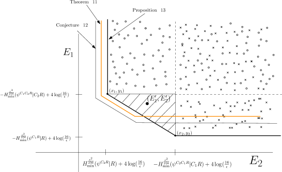
Figure 3: Entanglement cost for multiparty merging in the one-shot regime when $m=2$. The axes correspond to the entanglement cost $E_{1}:=\log K_{1}-\log L_{1}$ and $E_{2}:=\log K_{2}-\log L_{2}$. For $m=2$, we have two permutations of the set $\{1,2\}$, and according Proposition 13, two intersecting regions (circles and crosses) where existence of a $2$-party state merging of error $\epsilon$ can be shown.

VII A Worked Example

The proof of Theorem 11 is significantly more complicated than that of Proposition 13. To illustrate the benefits accruing from the additional effort, we will compare the two results’ estimates of the costs achievable for merging $C_{1}$ and $C_{2}$ to $R$ for states of the form

$$|\psi\rangle^{C_{1}C_{2}R}=\frac{1}{\sqrt{H_{d}}}\sum_{j=1}^{d}\frac{1}{\sqrt{j}}|j\rangle^{C_{1}}|\psi_{j}\rangle^{C_{2}}|j\rangle^{R},$$ (85)

where $H_{d}=\sum_{j=1}^{d}1/j$ is the $d$th harmonic number. These are close relatives of the embezzling states introduced in Hayden04 , which are useful resources for channel simulation and other tasks Harrow ; Berta02 ; Reverse . They make interesting examples because they have sufficient variation in their Schmidt coefficients that the i.i.d. state merging rates of Theorem 3 are not achievable in the one-shot regime. Nonetheless, our results yield nontrivial one-shot rates that are significantly better than simple teleportation. We will assume that $|\langle\psi_{i}|\psi_{j}\rangle|\leq\alpha$ for $i\neq j$ and try to and express the rates in terms of $\alpha$. We will assume for convenience that $\alpha>0$ since, when $\alpha=0$, the costs are essentially the same as when $\alpha=\Omega(1/d)$.

Protocols from Theorem 11

Let $(E_{1},E_{2})$ be a pair of entanglement costs achievable according to Theorem 11. The only constraints on the costs (aside from needing to be the logs of integers) are

$$E_{1} \geq -H_{\operatorname{min}}(\psi^{C_{1}R}|\psi^{R})+4\log(1/\epsilon)+12$$ (86)

$$E_{2} \geq -H_{\operatorname{min}}(\psi^{C_{2}R}|\psi^{R})+4\log(1/\epsilon)+12$$ (87)

$$E_{1}+E_{2} \geq -H_{\operatorname{min}}(\psi^{C_{1}C_{2}R}|\psi^{R})+4\log(1/\epsilon)+12.$$ (88)

To begin, we will find a sufficient condition for the $E_{1}$ constraint to be satisfied, so we need to evaluate $H_{\operatorname{min}}(\psi^{C_{1}R}|\psi^{R})$. Let $\lambda$ be the smallest real number such that $\lambda(I^{C_{1}}\otimes\psi^{R})-\psi^{C_{1}R}\geq 0$. Expanding the operators, that condition is the same as

$$\sum_{ij}\frac{\lambda-\delta_{ij}}{j}|ij\rangle\langle ij|^{C_{1}R}-\sum_{i}\sum_{j\neq i}\frac{1}{\sqrt{ij}}|ii\rangle\langle jj|^{C_{1}R}\langle\psi_{j}|\psi_{i}\rangle\geq 0,$$ (89)

where $\delta_{ij}$ is the Kronecker delta function. By the Gershgorin Circle Theorem Horn ; wiki , the operator will be positive semidefinite if each diagonal entry dominates the sum of the absolute values of the off-diagonal entries in the corresponding row. That condition reduces to

$$\frac{\lambda-1}{i}\geq\sum_{j\neq i}\frac{1}{\sqrt{ij}}|\langle\psi_{j}|\psi_{i}\rangle|$$ (90)

holding for all $i$, which is true provided $\lambda-1\geq\alpha\sum_{j=1}^{d}\sqrt{d/j}$. But

$$\sum_{j=1}^{d}\frac{1}{\sqrt{j}}\leq\int_{0}^{d}\frac{1}{\sqrt{x}}\,dx=2\sqrt{d}.$$ (91)

Therefore, the operator of eq. (89) will be positive semidefinite if $\lambda\geq 2\alpha d+1$. This in turn implies that

$$-H_{\operatorname{min}}(\psi^{C_{1}R}|\psi^{R})\leq\log(2\alpha d+1)\leq\log(\alpha d)+2.$$ (92)

The lower bound of eq. (86) will therefore be satisfied provided $E_{1}\geq\log(\alpha d)+4\log(1/\epsilon)+14$. The interpretation is that if the states $\{|\psi_{j}\rangle\}$ are indistinguishable, then $C_{1}$ holds the whole purification of $R$ and must therefore be responsible for the full cost of merging. As the states $\{|\psi_{j}\rangle\}$ become more distinguishable, the purification of $R$ becomes shared between $C_{1}$ and $C_{2}$, so the merging cost can be shared. Indeed, if $\alpha=O(1/d)$, then the lower bound on $E_{1}$ becomes a constant, independent of the size of the input state $|\psi\rangle^{C_{1}C_{2}R}$.

Moving on to the $E_{2}$ constraint, eq. (87), a similar but easier calculation shows that $H_{\operatorname{min}}(\psi^{C_{2}R}|\psi^{R})=0$. For the sum rate $E_{1}+E_{2}$, it is necessary to evaluate $H_{\operatorname{min}}(\psi^{C_{1}C_{2}R}|\psi^{R})$. Since the rank of $\psi^{C_{1}C_{2}}$ is $d$, this entropy is at least $-\log d$ Renner01 .

So any pair of costs $(E_{1},E_{2})$ satisfying

$$E_{1} \geq \log(\alpha d)+4\log(1/\epsilon)+14$$ (93)

$$E_{2} \geq 4\log(1/\epsilon)+12$$ (94)

$$E_{1}+E_{2} \geq \log d+4\log(1/\epsilon)+12$$ (95)

will be achievable by Theorem 11. The total cost $E_{1}+E_{2}$ must be at least $\log d$ plus terms independent of the size of $|\psi\rangle^{C_{1}C_{2}R}$ and that cost can be shared between $E_{1}$ and $E_{2}$. The lower bound on $E_{2}$ alone is independent of $d$ and should be regarded as a small “overhead” for the protocol. There is a minimal $d$-dependent cost for $E_{1}$, however, which encodes the fact that if $C_{2}$ does not carry enough of the purification of $R$ by virtue of the nonorthogonality of the $\{|\psi_{j}\rangle\}$, then more of the burden will fall to $C_{1}$.

VII.1 Protocols from Proposition 13

Now let us consider the costs achievable according to Proposition 13. For fixed $\epsilon$, the proposition provides two cost pairs, plus others that are simply degraded versions of those two arising from the wasteful consumption of unnecessary entanglement. Proposition 13 does not permit interpolation between the two points, as compared to Theorem 11. It might be the case, however, that Proposition 13’s freedom to smooth the entropy and vary the operator being conditioned upon could result in those two cost pairs being much better than any of those provided by Theorem 11. On the contrary, for the states of the example, the improvement achieved with the extra freedom is minimal.

Let $(E_{1}^{\prime},E_{2}^{\prime})$ be a cost pair achievable by Proposition 13. For the purposes of illustration, consider the point with the smallest possible value of $E_{2}^{\prime}$. Letting $\delta=\epsilon^{2}/256$, that point will satisfy

$$E_{1}^{\prime} \geq -H_{\operatorname{min}}^{\delta}(\psi^{C_{1}C_{2}R}|C_{2}R)+4\log\left(2/\epsilon\right)+12$$ (96)

$$E_{2}^{\prime} \geq -H_{\operatorname{min}}^{\delta}(\psi^{C_{2}R}|R)+4\log\left(2/\epsilon\right)+12.$$ (97)

Since the state $\psi^{C_{2}R}$ is separable, the cost $E_{2}^{\prime}$ cannot be negative, at least for sufficiently small $\epsilon$, so the key number is the $E_{1}^{\prime}$ cost. Before introducing the extra complication of smoothing, consider first $H_{\operatorname{min}}(\psi^{C_{1}C_{2}R}|C_{1}R)$. By Renner03 , this is related to the largest overlap that can be achieved with a maximally entangled state on $C_{2}/C_{1}R$ by acting with a quantum channel on the $C_{1}R$ part of $\psi^{C_{1}C_{2}R}$. This maximum singlet fraction is at least what is achieved by just aligning the Schmidt bases, which is

$$\left|\sum_{j=1}^{d}\frac{1}{\sqrt{j\cdot H_{d}}}\cdot\frac{1}{\sqrt{d}}\right|^{2} = \frac{1}{d\cdot H_{d}}\left|\sum_{j=1}^{d}\frac{1}{\sqrt{j}}\right|^{2}$$ (98)

$$\geq \frac{1}{d\cdot H_{d}}\left|\int_{1}^{d}\frac{1}{\sqrt{x}}dx\right|^{2}$$ (99)

$$= \frac{4}{H_{d}}\left(1-O\left(\frac{1}{\sqrt{d}}\right)\right)$$ (100)

$$\geq \frac{5}{\log d},$$ (101)

where the last line holds for sufficiently large $d$. Above and in what follows, we use the inequality $\ln(d+1)\leq H_{d}\leq(\ln d)+1$, which was supplemented above by the fact that $4/(\ln d+1)\geq 5.7/\log d$ for sufficiently large $d$. According to Theorem 2 of Renner03 , the resulting bound on $H_{\operatorname{min}}$ is

$$-H_{\operatorname{min}}(\psi^{C_{1}C_{2}R}|RC_{2})\geq\log d-\log\log d+2.$$ (102)

Therefore, ignoring smoothing, the sum cost for Proposition 13 will always satisfy

$$E_{1}^{\prime}+E_{2}^{\prime}\geq\log d-\log\log d+26+8\log\left(\frac{2}{\epsilon}\right),$$ (103)

for sufficiently large $d$, which has worse constants and even asymptotically only differs from the sum cost (95) for Theorem 11 by $O(\log\log d)$.

Now let us introduce some smoothing. By duality of the min- and max- entropies,

$$-H^{\delta}_{\operatorname{min}}(\psi^{C_{1}C_{2}R}|RC_{2})=H^{\delta}_{\operatorname{max}}(\psi^{C_{1}}).$$ (104)

Lemma 25 of Appendix C gives that

$$H^{\delta}_{\operatorname{max}}(\psi^{C_{1}})\geq 2\log{\operatorname{min}}\left\{\sum_{j=1}^{k-1}\frac{1}{\sqrt{j\cdot H_{d}}}:k\mbox{ such that }\sum_{j=k+1}^{d}\frac{1}{j\cdot H_{d}}\leq\frac{\delta^{2}}{2}\right\}.$$ (105)

Getting a lower bound on this expression requires finding large $k$ that nonetheless fail to satisfy the tail condition. That restriction on $k$ is equivalent to $1-H_{k}/H_{d}\leq\delta^{2}/2$, which will not be met by any $k$ small enough to obey

$$k\leq(d+1)^{1-\delta^{2}/2}/e$$ (106)

for sufficiently large $d$. Using a similar estimate as for the maximum singlet fraction calculation, we get

$$2\log\sum_{j=1}^{k-1}\frac{1}{\sqrt{j\cdot H_{d}}} \geq \log\left(\frac{1}{\sqrt{H_{d}}}\int_{1}^{k}\frac{1}{\sqrt{x}}\,dx\right)^{2}$$ (107)

$$\geq \log\frac{4k}{H_{d}}\left(1-O\left(\frac{1}{\sqrt{k}}\right)\right)$$ (108)

$$\geq \log k-\log\log d+\log 5$$ (109)

for sufficiently large $k$. Substituting in the largest possible $k$ consistent with eq. (106) and $\delta=\epsilon^{2}/256$ gives

$$E_{1}^{\prime}+E_{2}^{\prime}\geq\left(1-\frac{\epsilon^{4}}{512}\right)\log(d+1)-\log\log d+24+8\log\left(\frac{2}{\epsilon}\right),$$ (110)

for sufficiently large $d$. The sum costs achievable using Theorem 11 compare favorably with this bound. The additional savings from smoothing are only about $\epsilon^{4}\log(d+1)/512$ ebits, which is insignificant for small $\epsilon$. These tiny savings also come at the expense of being able to interpolate between achievable costs. To be fair, these states were chosen specifically because they are known to maintain their essential character even after smoothing, as was observed in Hayden05 . The freedom to smooth is certainly more beneficial for some other classes of states, most notably i.i.d. states. Indeed, since $S(\psi^{C_{1}C_{2}})=(\log d)/2+O(\log\log d)$, merging many copies of $|\psi\rangle^{C_{1}C_{2}R}$ can be done at a rate roughly half the cost required for one-shot merging.

VIII A variant of Merging: Split Transfer

In the previous sections, we’ve analyzed and characterized the entanglement cost for merging the state $\psi^{C_{1}C_{2}\ldots C_{m}BR}$ to a single receiver Bob in the asymptotic setting and in the one-shot regime. Here, we modify our initial setup by introducing a second decoder $A$ (Alice), who is spatially separated from Bob and also has side information about the input state. That is, the helpers $C_{1},C_{2},\ldots,C_{m}$ and the two receivers Alice and Bob share a global state $\psi^{C_{1}C_{2}\ldots C_{m}ABR}$ and the objective is then to redistribute the state $\psi^{C_{1}C_{2}\ldots C_{m}ABR}$ to Alice, Bob, and the reference $R$. The motivation for this problem comes from the multipartite entanglement of assistance problem SVW ; Merge , where the task is to distill entanglement in the form of EPR pairs from a $(m+2)$-partite pure state $\psi^{C_{1}C_{2}\ldots C_{m}AB}$ shared between two recipients (Alice and Bob) and $m$ other helpers $C_{1},C_{2},\ldots,C_{m}$. If many copies of the input state are available, the optimal EPR rate was shown in Merge to be equal to

$$E^{\infty}_{A}(\psi^{C_{1}C_{2}\ldots C_{m}AB}):={\operatorname{min}}_{\cal T}S(A{\cal T})_{\psi},$$ (111)

where ${\cal T}\subseteq\{C_{1},C_{2},\ldots,C_{m}\}$ is a subset (i.e a bipartite cut) of the helpers. We denote the complement by $\overline{\cal T}:=\{C_{1}C_{2}\ldots C_{m}\}\setminus{\cal T}$. We call ${\operatorname{min}}_{\cal T}\{S(A{\cal T})_{\psi}\}$ the minimum cut (min-cut) entanglement of the state $\psi^{C_{1}C_{2}\ldots C_{m}AB}$.

The proof that the rate given by eq. (111) is achievable using LOCC operations consists of showing that the min-cut entanglement of the state $\psi^{C_{1}C_{2}\ldots C_{m}AB}$ is preserved, up to an arbitrarily small variation, after each sender has finished performing a random measurement on his system. The procedure described in the proof of Merge makes use of a multiple-blocking strategy. That is, given $n$ copies of the input state $\psi^{C_{1}C_{2}\ldots C_{m}AB}$, the first helper will perform $d=n/m$ random measurements, each acting on $m$ copies of $\psi^{C_{1}C_{2}\ldots C_{m}AB}$ and generating $J$ possible outcomes. Then, if each measurement can yield outcomes $j_{1},j_{2},\ldots,j_{d}$, we need to group together the residual states corresponding to outcome $1$, then group the ones corresponding to outcome $2$, etc… When this is done, the next helper will perform random measurements for each of these groups in the same way the first sender proceeded. That is, for each group, you need to divide into blocks, and so on. Needless to say, this approach fails in the one-shot setting.

It was conjectured in Merge that these layers of blocking could be removed by letting all the helpers perform simultaneous measurements on their respective typical subspaces. Such a strategy would still produce states which preserve the min-cut entanglement, thereby providing a way to prove eq. (111) without the need for a recursive argument. We will show in the remainder of this section that for a cut ${\cal T}_{{\operatorname{min}}}$ which minimizes $S(A{\cal T})_{\psi}$, there exists an LOCC protocol acting on the state $\psi^{C_{1}C_{2}\ldots C_{m}BR}$ which will send ${\cal T}_{{\operatorname{min}}}$ to Alice and its complement to Bob. The protocol will consist of two parts. First, all the helpers will perform measurements on their typical subspaces and broadcast their outcomes to both decoders. Then, Alice will use the classical information coming from the helpers which are part of the cut ${\cal T}_{{\operatorname{min}}}$ and apply an isometry $U$, while Bob will apply an isometry $V$ depending on the outcomes of the helpers belonging to $\overline{\cal T}_{{\operatorname{min}}}$. This will redistribute the initial state to Alice, Bob, and the reference $R$. Standard distillation protocols Concentrate ; Bennett on the recovered state will yield EPR pairs at a rate given by eq. (111).

Definition 14

Let $\psi^{{\cal T}{\overline{\cal T}}ABR}$ be an $(m+2)$-partite state, where ${\cal T}$ and $\overline{\cal T}$ are a partition of the helpers $C_{1},C_{2},\ldots,C_{m}$. Furthermore, assume that the helpers and the decoders share maximally entangled states $\Phi^{K}:=\bigotimes_{i\in\cal T}\Phi^{K_{i}}$ and $\Gamma^{M}:=\bigotimes_{i\in\overline{\cal T}}\Gamma^{M_{i}}$ on the tensor product spaces ${\cal T}^{0}A^{0}_{{\cal T}}$ and $\overline{{\cal T}^{0}}B^{0}_{\overline{\cal T}}$.

We call the LOCC operation ${\cal M}:{\cal T}{\cal T}^{0}\overline{\cal T}\overline{{\cal T}^{0}}\otimes AA^{0}_{{\cal T}}\otimes BB^{0}_{\overline{{\cal T}}}\rightarrow{\cal T}^{1}A^{1}_{{\cal T}}AA_{{\cal T}}\otimes{\overline{\cal T}}^{1}B^{1}_{\overline{{\cal T}}}BB_{\overline{{\cal T}}}$ a split transfer of the state $\psi^{{\cal T}{\overline{\cal T}}ABR}$ with error $\epsilon$ and associated entanglement costs $\overrightarrow{E_{{\cal T}}}(\psi):=\bigoplus_{i\in{\cal T}}(\log K_{i}-\log L_{i})$ and $\overrightarrow{E_{{\overline{\cal T}}}}(\psi):=\bigoplus_{i\in{\overline{\cal T}}}(\log M_{i}-\log N_{i})$ if

$$\bigg{\|}(\mathrm{id}_{R}\otimes{\cal M})(\psi^{{\cal T}{\overline{\cal T}}ABR}\otimes\Phi^{K}\otimes\Gamma^{M})-\psi_{AA_{{\cal T}}BB_{\overline{\cal T}}R}\otimes\Phi^{L}\otimes\Gamma^{N}\bigg{\|}_{1}\leq\epsilon,$$ (112)

where $\Phi^{L}:=\bigotimes_{i\in{\cal T}}\Phi^{L_{i}},\Gamma^{N}:=\bigotimes_{j\in{\overline{\cal T}}}\Gamma^{N_{j}}$, with the states $\Phi^{L_{i}}$ and $\Gamma^{N_{j}}$ being maximally entangled states of Schmidt ranks $L_{i}$ and $N_{i}$ on $C^{1}_{i}A^{1}_{i}$ and $C_{j}^{1}B^{1}_{j}$ respectively. Also, the systems $A_{\cal T}$ and $B_{\overline{\cal T}}$ are ancillary systems of the same size as ${\cal T}$ and ${\overline{\cal T}}$ and are held by Alice and Bob respectively. For the state $\Psi:=(\psi^{{\cal T}{\overline{\cal T}}ABR})^{\otimes n}$, the entanglement rates $\overrightarrow{R_{{\cal T}}}(\psi)$ and $\overrightarrow{R_{{\overline{\cal T}}}}(\psi)$ are defined as $\frac{1}{n}\overrightarrow{E_{{\overline{\cal T}}}}(\Psi)$ and $\frac{1}{n}\overrightarrow{E_{{\overline{\cal T}}}}(\Psi)$.

In the above definition, we have denoted by $\bigoplus_{i\in{\cal T}}(\log K_{i}-\log L_{i})$ a vector of length $|{\cal T}|$ whose components are given by $\log K_{i}-\log L_{i}$ for $i\in{\cal T}$ in the lexicographical order.

The rate region where a split-transfer can be accomplished by LOCC can be defined in a manner analogous to definition 2. We omit the details here, but whenever we will say that a rate is achievable for a split-transfer of the state $\psi^{{\cal T}{\overline{\cal T}}ABR}$, it will mean that it is contained in the rate region.

Now, we’d like to specify conditions, as in Proposition 4, that the initial state should satisfy in order to allow the group ${\cal T}$ (resp. ${\overline{\cal T}}$) to transfer their share of the state to Alice (resp. Bob). For a pure state $\psi^{{\cal T}{\overline{\cal T}}ABR}$, suppose all the helpers perform incomplete measurements (as in Section III) on their respective shares of the state. For measurement outcomes $J:=(j_{1},j_{2},\ldots,j_{m})$, define the state

$$\begin{split}|\psi_{J}^{{\cal T}^{1}\overline{{\cal T}^{1}}ABR}\rangle&:=\frac{1}{\sqrt{p_{J}}}(P^{1}_{j_{1}}\otimes P^{2}_{j_{2}}\otimes\ldots\otimes P^{m}_{j_{m}}\otimes I^{ABR})|\psi^{{\cal T}{\overline{\cal T}}ABR}\rangle\\ &=:\frac{1}{\sqrt{p_{J}}}(P^{{\cal T}}_{j_{{\cal T}}}\otimes P^{{\overline{\cal T}}}_{j_{{\overline{\cal T}}}}\otimes I^{ABR})|\psi^{{\cal T}{\overline{\cal T}}ABR}\rangle,\\ \end{split}$$ (113)

where $p_{J}$ is the probability of getting outcome $J$. In the above definition, $j_{{\cal T}}$ is a vector of length $|{\cal T}|$ whose components correspond to outcomes of measurements performed by the helpers belonging to the cut ${\cal T}$. The vector $j_{{\overline{\cal T}}}$ is defined similarly. Finally, the Kraus operators $P^{{\cal T}}_{j_{{\cal T}}}=\bigotimes_{i\in{\cal T}}P^{i}_{j_{i}}$ and $P^{{\overline{\cal T}}}_{j_{{\overline{\cal T}}}}=\bigotimes_{i\in{\overline{\cal T}}}P^{i}_{j_{i}}$ map the spaces ${\cal T}$ and ${\overline{\cal T}}$ to the subspaces ${\cal T}^{1}$ and $\overline{{\cal T}^{1}}$ respectively.

Define another state $|\varphi_{j_{{\cal T}}}^{{\cal T}^{1}{\overline{\cal T}}ABR}\rangle:=\frac{1}{\sqrt{p_{j_{{\cal T}}}}}(P^{{\cal T}}_{j_{{\cal T}}}\otimes I^{{\overline{\cal T}}ABR})|\psi^{{\cal T}{\overline{\cal T}}ABR}\rangle$, where $p_{j_{{\cal T}}}$ is the probability of getting the outcome $j_{{\cal T}}$, and suppose that we have

$$\varphi_{j_{{\cal T}}}^{{\cal T}^{1}{\overline{\cal T}}BR}=\tau_{L}^{{\cal T}^{1}}\otimes\psi^{{\overline{\cal T}}BR},$$ (114)

where $\tau_{L}^{{\cal T}^{1}}=\bigotimes_{i\in{\cal T}}\tau^{C^{1}_{i}}$ is the maximally mixed state of dimension $L$ on the system ${\cal T}^{1}$. From the Schmidt decomposition, we know there exists an isometry $U^{A}_{j_{{\cal T}}}:A\rightarrow A^{1}_{{\cal T}}A_{{\cal T}}A$ which Alice can perform such that

$$(I^{{\cal T}^{1}{\overline{\cal T}}BR}\otimes U^{A}_{j_{{\cal T}}})|\varphi_{j_{{\cal T}}}^{{\cal T}^{1}{\overline{\cal T}}ABR}\rangle=|\Phi^{L}\rangle\otimes|\psi^{A_{{\cal T}}{\overline{\cal T}}ABR}\rangle,$$ (115)

where the state $|\psi^{A_{{\cal T}}{\overline{\cal T}}ABR}\rangle$ is the same as the original state $|\psi^{{\cal T}{\overline{\cal T}}ABR}\rangle$ with the ancillary system $A_{{\cal T}}$ substituted for ${\cal T}$. The state $|\Phi^{L}\rangle$ is a maximally entangled state on ${\cal T}^{1}A^{1}_{{\cal T}}$.

Finally, define the state $|\upsilon_{j_{{\overline{\cal T}}}}^{A_{{\cal T}}\overline{{\cal T}^{1}}ABR}\rangle:=\frac{1}{\sqrt{p_{j_{{\overline{\cal T}}}}}}(P^{{\overline{\cal T}}}_{j_{{\overline{\cal T}}}}\otimes I_{A_{{\cal T}}ABR})|\psi^{A_{{\cal T}}{\overline{\cal T}}ABR}\rangle$ and suppose again that we have

$$\upsilon_{j_{{\overline{\cal T}}}}^{A_{{\cal T}}\overline{{\cal T}^{1}}AR}=\tau_{N}^{\overline{{\cal T}^{1}}}\otimes\psi^{A_{{\cal T}}AR},$$ (116)

where $\tau_{N}^{\overline{{\cal T}^{1}}}=\bigotimes_{i\in{\overline{\cal T}}}\tau^{C^{1}_{i}}$ is the maximally mixed state of dimension $N$ on the system $\overline{{\cal T}^{1}}$. Applying the Schmidt decomposition once more, Bob can perform an isometry $V^{B}_{j_{{\overline{\cal T}}}}:B\rightarrow B^{1}_{{\overline{\cal T}}}B_{{\overline{\cal T}}}B$ such that

$$(I^{A_{{\cal T}}\overline{{\cal T}^{1}}AR}\otimes V^{B}_{j_{{\overline{\cal T}}}})|\upsilon_{j_{{\overline{\cal T}}}}^{A_{{\cal T}}\overline{{\cal T}^{1}}ABR}\rangle=|\Gamma^{N}\rangle\otimes|\psi^{A_{{\cal T}}B_{{\overline{\cal T}}}ABR}\rangle,$$ (117)

where the state $|\psi^{A_{{\cal T}}B_{{\overline{\cal T}}}ABR}\rangle$ is the same as the original state $\psi^{{\cal T}{\overline{\cal T}}ABR}$ with the ancillary systems $A_{{\cal T}}$ and $B_{{\overline{\cal T}}}$ substituted for ${\cal T}$ and ${\overline{\cal T}}$.

If we apply the isometries $U^{A}_{j_{{\cal T}}}$ and $V^{B}_{j_{{\overline{\cal T}}}}$ to the outcome state $|\psi_{J}^{{\cal T}^{1}\overline{{\cal T}^{1}}ABR}\rangle$, the resulting state is given by

$$\begin{split}&(I^{{\cal T}^{1}\overline{{\cal T}^{1}}R}\otimes U^{A}_{j_{{\cal T}}}\otimes V^{B}_{j_{{\overline{\cal T}}}})|\psi_{J}^{{\cal T}^{1}\overline{{\cal T}^{1}}ABR}\rangle\\ &=\frac{1}{\sqrt{p_{J}}}(I^{{\cal T}^{1}\overline{{\cal T}^{1}}R}\otimes U^{A}_{j_{{\cal T}}}\otimes V^{B}_{j_{{\overline{\cal T}}}})(P^{{\overline{\cal T}}}_{j_{{\overline{\cal T}}}}\otimes I^{{\cal T}^{1}ABR})(P^{{\cal T}}_{j_{{\cal T}}}\otimes I^{{\overline{\cal T}}ABR})|\psi^{{\cal T}{\overline{\cal T}}ABR}\rangle\\ &=\frac{1}{\sqrt{p_{J}}}(I^{{\cal T}^{1}A^{1}_{{\cal T}}A_{{\cal T}}\overline{{\cal T}^{1}}AR}\otimes V^{B}_{j_{{\overline{\cal T}}}})(P^{{\overline{\cal T}}}_{j_{{\overline{\cal T}}}}\otimes I^{{\cal T}^{1}A^{1}_{{\cal T}}A_{{\cal T}}ABR})(I^{{\cal T}^{1}BR}\otimes U^{A}_{j_{{\cal T}}})(P^{{\cal T}}_{j_{{\cal T}}}\otimes I^{{\overline{\cal T}}ABR})|\psi^{{\cal T}{\overline{\cal T}}ABR}\rangle\\ &=\frac{1}{\sqrt{p_{J}}}(I^{{\cal T}^{1}A^{1}_{{\cal T}}A_{{\cal T}}\overline{{\cal T}^{1}}AR}\otimes V^{B}_{j_{{\overline{\cal T}}}})(P^{{\overline{\cal T}}}_{j_{{\overline{\cal T}}}}\otimes I^{{\cal T}^{1}A^{1}_{{\cal T}}A_{{\cal T}}ABR})(I^{{\cal T}^{1}BR}\otimes U^{A}_{j_{{\cal T}}})\sqrt{p_{j_{{\cal T}}}}|\varphi_{j_{{\cal T}}}^{{\cal T}^{1}{\overline{\cal T}}ABR}\rangle\\ &=\sqrt{\frac{p_{j_{{\cal T}}}}{p_{J}}}(I^{{\cal T}^{1}A^{1}_{{\cal T}}A_{{\cal T}}\overline{{\cal T}^{1}}AR}\otimes V^{B}_{j_{{\overline{\cal T}}}})(P^{{\overline{\cal T}}}_{j_{{\overline{\cal T}}}}\otimes I^{{\cal T}^{1}A^{1}_{{\cal T}}A_{{\cal T}}ABR})|\Phi^{L}\rangle\otimes|\psi^{AA_{{\cal T}}{\overline{\cal T}}BR}\rangle\\ &=\sqrt{\frac{p_{j_{{\cal T}}}}{p_{J}}}(I^{{\cal T}^{1}A^{1}_{{\cal T}}A_{{\cal T}}\overline{{\cal T}^{1}}AR}\otimes V^{B}_{j_{{\overline{\cal T}}}})|\Phi^{L}\rangle\otimes\sqrt{p_{j_{{\overline{\cal T}}}}}|\upsilon_{j_{{\overline{\cal T}}}}^{A_{{\cal T}}\overline{{\cal T}^{1}}ABR}\rangle\\ &=\sqrt{\frac{p_{j_{{\cal T}}}p_{j_{{\overline{\cal T}}}}}{p_{J}}}|\Phi^{L}\rangle\otimes|\Gamma^{N}\rangle\otimes|\psi^{AA_{{\cal T}}B_{{\overline{\cal T}}}BR}\rangle.\\ \end{split}$$ (118)

Since the states $(I^{{\cal T}^{1}\overline{{\cal T}^{1}}R}\otimes U^{A}_{j_{{\cal T}}}\otimes V^{B}_{j_{{\overline{\cal T}}}})|\psi_{J}^{{\cal T}^{1}\overline{{\cal T}^{1}}ABR}\rangle$ and $|\Phi^{L}\rangle\otimes|\Gamma^{N}\rangle\otimes|\psi^{AA_{{\cal T}}B_{{\overline{\cal T}}}BR}\rangle$ are both normalized, we must have $p_{J}=p_{j_{{\cal T}}}p_{j_{{\overline{\cal T}}}}$. Hence, in this ideal case, we can achieve a split transfer of the state $\psi^{C_{1}C_{2}\ldots C_{m}BR}$ by letting all the helpers measure their share simultaneously. The decoding by Alice and Bob will follow once they receive the measurement outcomes.

Proposition 15 (Conditions for a Split-Transfer)

Denote the state shared between $m$ helpers and two receivers (Alice and Bob) by $\psi^{{\cal T}{\overline{\cal T}}ABR}$, with purifying system $R$. Suppose all the helpers perform incomplete measurements on their share of the state $\psi^{{\cal T}{\overline{\cal T}}ABR}$ as in the previous paragraphs, yielding a state $|\psi_{J}^{{\cal T}^{1}\overline{{\cal T}^{1}}ABR}\rangle:=\frac{1}{\sqrt{p_{J}}}(P^{{\cal T}}_{j_{{\cal T}}}\otimes P^{{\overline{\cal T}}}_{j_{{\overline{\cal T}}}}\otimes I^{ABR})(|\psi^{{\cal T}{\overline{\cal T}}ABR}\rangle)$ for an outcome $J:=(j_{1},j_{2},\ldots,j_{m})$ with probability $p_{J}$, where the Kraus operators $P^{{\cal T}}_{j_{{\cal T}}}$ and $P^{{\overline{\cal T}}}_{j_{{\overline{\cal T}}}}$ map the spaces ${\cal T}$ and ${\overline{\cal T}}$ to the subspaces ${\cal T}^{1}$ and $\overline{{\cal T}^{1}}$.

If, for the quantum errors $Q^{1}_{\cal I}(\psi^{{\cal T}{\overline{\cal T}}ABR})$ and $Q^{2}_{\cal I}(\psi^{{\cal T}{\overline{\cal T}}ABR})$, we have

$$\begin{split}Q^{1}_{\cal I}(\psi^{{\cal T}{\overline{\cal T}}ABR})&:=\sum_{j_{{\cal T}}}p_{j_{{\cal T}}}\|\varphi_{j_{{\cal T}}}^{{\cal T}^{1}{\overline{\cal T}}BR}-\tau^{{\cal T}^{1}}_{L}\otimes\psi^{{\overline{\cal T}}BR}\|_{1}\leq\epsilon\\ Q^{2}_{\cal I}(\psi^{{\cal T}{\overline{\cal T}}ABR})&:=\sum_{j_{{\overline{\cal T}}}}p_{j_{{\overline{\cal T}}}}\|\upsilon_{j_{{\overline{\cal T}}}}^{A_{{\cal T}}\overline{{\cal T}^{1}}AR}-\tau^{\overline{{\cal T}^{1}}}_{N}\otimes\psi^{A_{{\cal T}}AR}\|_{1}\leq\epsilon^{\prime},\\ \end{split}$$ (119)

then there exists a split-transfer of the state $\psi^{{\cal T}{\overline{\cal T}}ABR}$ with error $2\sqrt{\epsilon}+2\sqrt{\epsilon^{\prime}}$ and entanglement costs $\overrightarrow{E_{{\cal T}}}=\bigoplus_{i\in{\cal T}}(-\log L_{i})$ and $\overrightarrow{E_{{\overline{\cal T}}}}=\bigoplus_{i\in{\overline{\cal T}}}(-\log N_{i})$. The states $\varphi_{j_{{\cal T}}}^{{\cal T}^{1}{\overline{\cal T}}BR}$ and $\upsilon_{j_{{\overline{\cal T}}}}^{A_{{\cal T}}\overline{{\cal T}^{1}}AR}$ are reduced density operators for the states $|\varphi_{j_{{\cal T}}}^{{\cal T}^{1}{\overline{\cal T}}ABR}\rangle:=\frac{1}{\sqrt{p_{j_{{\cal T}}}}}(P^{{\cal T}}_{j_{{\cal T}}}\otimes I^{{\overline{\cal T}}ABR})|\psi^{{\cal T}{\overline{\cal T}}ABR}\rangle$ and $|\upsilon_{j_{{\overline{\cal T}}}}^{A_{{\cal T}}\overline{{\cal T}^{1}}ABR}\rangle:=\frac{1}{\sqrt{p_{j_{{\overline{\cal T}}}}}}(P^{{\overline{\cal T}}}_{j_{{\overline{\cal T}}}}\otimes I^{A_{{\cal T}}ABR})|\psi^{A_{{\cal T}}{\overline{\cal T}}ABR}\rangle$.

Proof.

Since the quantum errors $Q^{1}_{\cal I}$ and $Q^{2}_{\cal I}$ are bounded from above by $\epsilon$ and $\epsilon^{\prime}$ respectively, Proposition 4 can be applied, which tells us of the existence of isometries $U^{A}_{j_{{\cal T}}}$ and $V^{B}_{j_{{\overline{\cal T}}}}$ such that

$$\begin{split}\bigg{\|}\sum_{j_{{\cal T}}}p_{j_{{\cal T}}}(I^{{\overline{\cal T}}BR}\otimes U^{A}_{j_{{\cal T}}})|\varphi^{{\cal T}^{1}{\overline{\cal T}}ABR}_{j_{{\cal T}}}\rangle\langle\varphi^{{\cal T}^{1}{\overline{\cal T}}ABR}_{j_{{\cal T}}}|(I^{{\overline{\cal T}}BR}\otimes U^{A}_{j_{{\cal T}}})^{{\dagger}}-\psi^{A_{{\cal T}}{\overline{\cal T}}ABR}\otimes\Phi^{L}\bigg{\|}_{1}&\leq 2\sqrt{\epsilon}\\ \bigg{\|}\sum_{j_{{\overline{\cal T}}}}p_{j_{{\overline{\cal T}}}}(I^{A_{{\cal T}}AR}\otimes V^{B}_{j_{{\overline{\cal T}}}})|\upsilon^{A_{{\cal T}}\overline{{\cal T}^{1}}ABR}_{j_{{\overline{\cal T}}}}\rangle\langle\upsilon^{A_{{\cal T}}\overline{{\cal T}^{1}}ABR}_{j_{{\overline{\cal T}}}}|(I^{A_{{\cal T}}AR}\otimes V^{B}_{j_{{\overline{\cal T}}}})^{{\dagger}}-\psi^{A_{{\cal T}}B_{{\overline{\cal T}}}ABR}\otimes\Gamma^{N}\bigg{\|}_{1}&\leq 2\sqrt{\epsilon^{\prime}}.\\ \end{split}$$ (120)

If we apply the isometries $U^{A}_{j_{{\cal T}}}$ and $V^{B}_{j_{{\overline{\cal T}}}}$ to the state $|\psi^{{\cal T}^{1}\overline{{\cal T}^{1}}ABR}_{J}\rangle$ after obtaining outcome $J$, the output state $\rho$ of the protocol will be of the form

$$\begin{split}&\rho:=\sum_{J}p_{J}\bigg{(}(I^{{\cal T}^{1}\overline{{\cal T}^{1}}R}\otimes U^{A}_{j_{{\cal T}}}\otimes V^{B}_{j_{{\overline{\cal T}}}})\psi^{{\cal T}^{1}\overline{{\cal T}^{1}}ABR}_{J}(I^{{\cal T}^{1}\overline{{\cal T}^{1}}R}\otimes U^{A}_{j_{{\cal T}}}\otimes V^{B}_{j_{{\overline{\cal T}}}})^{{\dagger}}\bigg{)}\\ &=\sum_{J}p_{J}\bigg{(}\frac{p_{j_{{\cal T}}}}{p_{J}}(I\otimes V^{B}_{j_{{\overline{\cal T}}}})(P^{{\overline{\cal T}}}_{j_{{\overline{\cal T}}}}\otimes I)(I\otimes U^{A}_{j_{{\cal T}}})|\varphi_{j_{{\cal T}}}^{{\cal T}^{1}{\overline{\cal T}}ABR}\rangle\langle\varphi_{j_{{\cal T}}}^{{\cal T}^{1}{\overline{\cal T}}ABR}|(I\otimes U^{A}_{j_{{\cal T}}})^{{\dagger}}(P^{{\overline{\cal T}}}_{j_{{\overline{\cal T}}}}\otimes I)^{{\dagger}}(I\otimes V^{B}_{j_{{\overline{\cal T}}}})^{{\dagger}}\bigg{)}\\ &=\sum_{j_{{\overline{\cal T}}}}(I\otimes V^{B}_{j_{{\overline{\cal T}}}})(P^{{\overline{\cal T}}}_{j_{{\overline{\cal T}}}}\otimes I)\zeta(P^{{\overline{\cal T}}}_{j_{{\overline{\cal T}}}}\otimes I)^{{\dagger}}(I\otimes V^{B}_{j_{{\overline{\cal T}}}})^{{\dagger}}\\ &=:{\cal M}(\zeta)\\ \end{split}$$ (121)

where $\zeta:=\sum_{j_{{\cal T}}}p_{j_{{\cal T}}}(I\otimes U^{A}_{j_{{\cal T}}})|\varphi_{j_{{\cal T}}}^{{\cal T}^{1}{\overline{\cal T}}ABR}\rangle\langle\varphi_{j_{{\cal T}}}^{{\cal T}^{1}{\overline{\cal T}}ABR}|(I\otimes U^{A}_{j_{{\cal T}}})^{{\dagger}}$. It can be seen as the output state we would get if only the helpers in ${\cal T}$ wanted to transfer their share of the state to the decoder $A$. The map ${\cal M}$, as defined above, corresponds to an LOCC quantum operation acting on $\zeta$ which consists of measurements by the helpers in ${{\overline{\cal T}}}$ followed by an isometry on $B$. Note that we have remove some of the superscript notation for the sake of clarity.

We would like to bound the trace distance between the output state $\rho$ and the state $\psi^{A_{{\cal T}}B_{{\overline{\cal T}}}ABR}\otimes\Phi^{L}\otimes\Gamma^{N}$. To achieve this, we introduce the following intermediate state

$$\begin{split}\sigma&:=\sum_{j_{{\overline{\cal T}}}}(I\otimes V^{B}_{j_{{\overline{\cal T}}}})(P^{{\overline{\cal T}}}_{j_{{\overline{\cal T}}}}\otimes I)(\psi^{A_{{\cal T}}{\overline{\cal T}}ABR}\otimes\Phi^{L})(P^{{\overline{\cal T}}}_{j_{{\overline{\cal T}}}}\otimes I)^{{\dagger}}(I\otimes V^{B}_{j_{{\overline{\cal T}}}})^{{\dagger}}\\ &={\cal M}(\psi^{A_{{\cal T}}{\overline{\cal T}}ABR}\otimes\Phi^{L})\\ \end{split}$$ (122)

and apply the triangle inequality

$$\begin{split}\bigg{\|}\rho-&\psi^{A_{{\cal T}}B_{{\overline{\cal T}}}ABR}\otimes\Phi^{L}\otimes\Gamma^{N}\bigg{\|}_{1}\leq\bigg{\|}\rho-\sigma\bigg{\|}_{1}+\bigg{\|}\sigma-\psi^{A_{{\cal T}}B_{{\overline{\cal T}}}ABR}\otimes\Phi^{L}\otimes\Gamma^{N}\bigg{\|}_{1}.\\ \end{split}$$ (123)

The trace norm $\bigg{\|}\sigma-\psi^{A_{{\cal T}}B_{{\overline{\cal T}}}ABR}\otimes\Phi^{L}\otimes\Gamma^{N}\bigg{\|}_{1}$ is equal to the trace norm appearing in the second line of eq. (120), and so is bounded from above by $2\sqrt{\epsilon^{\prime}}$. To bound $\bigg{\|}\rho-\sigma\bigg{\|}_{1}$, we have

$$\begin{split}\bigg{\|}\rho-\sigma\bigg{\|}_{1}&=\bigg{\|}{\cal M}(\zeta)-{\cal M}(\psi^{A_{{\cal T}}{\overline{\cal T}}ABR}\otimes\Phi^{L})\bigg{\|}_{1}\\ &\leq\bigg{\|}\zeta-\psi^{A_{{\cal T}}{\overline{\cal T}}ABR}\otimes\Phi^{L}\bigg{\|}_{1}\\ &\leq 2\sqrt{\epsilon}.\end{split}$$ (124)

The first inequality holds since the trace distance is non-increasing under quantum operations, and the second inequality is just the first part of eq. (120). Thus, we have a split-transfer of the state $\psi^{C_{1}C_{2}\ldots C_{m}ABR}$ with error $2\sqrt{\epsilon}+2\sqrt{\epsilon^{\prime}}$.     $\sqcap$$\sqcup$

With this result in hand, a one-shot split-transfer protocol of the state $\psi^{{\cal T}{\overline{\cal T}}ABR}$ where all the helpers perform simultaneous random measurements on their share can be obtained by two independent applications of Proposition 5 followed by an application of Proposition 15. We state the result here.

Proposition 16 (One-Shot Split-Transfer)

Let $\psi^{{\cal T}{\overline{\cal T}}ABR}$ be an $(m+2)$-partite pure state, with purifying system $R$ and local dimensions $d_{A},d_{B},d_{R}$. Furthermore, let $d_{{\cal T}}:=\Pi_{i\in{\cal T}}d_{C_{i}}$ and $d_{{\overline{\cal T}}}:=\Pi_{i\in{\overline{\cal T}}}d_{C_{i}}$ be the dimensions of the systems ${\cal T}$ and ${\overline{\cal T}}$. Finally, allow the helpers to share additional maximally entangled states $\Phi^{K}$ and $\Gamma^{M}$ with the decoders.

For each party $C_{i}$ in the cut ${\cal T}$, there exists an instrument ${\cal I}_{i}=\{{\cal E}^{i}_{j}\}_{j=0}^{F_{i}}$ consisting of $F_{i}=\lfloor\frac{d_{C_{i}}K_{i}}{L_{i}}\rfloor$ partial isometries of rank $L_{i}$ and one of rank $L_{i}^{\prime}=d_{C_{i}}K_{i}-F_{i}L_{i}<L_{i}$ such that the overall quantum error $Q^{1}_{{\cal I}}(\psi^{{\cal T}{\overline{\cal T}}ABR}\otimes\Phi^{K})$ is bounded by

$$\begin{split}Q^{1}_{\cal I}(\psi^{{\cal T}{\overline{\cal T}}ABR}\otimes\Phi^{K})&\leq 2\sum_{\begin{subarray}{c}{\cal S}\subseteq{\cal T}\\ {\cal S}\neq\emptyset\end{subarray}}\prod_{i\in{\cal S}}\frac{L_{i}}{d_{C_{i}}K_{i}}+2\sqrt{d_{{\overline{\cal T}}}d_{B}d_{R}\sum_{\begin{subarray}{c}{\cal S}\subseteq{\cal T}\\ {\cal S}\neq\emptyset\end{subarray}}\prod_{i\in{\cal S}}\frac{L_{i}}{K_{i}}\mathrm{Tr}\bigg{[}(\psi^{{\cal S}{\overline{\cal T}}BR})^{2}\bigg{]}}=:\Delta^{1}_{\cal I}.\\ \end{split}$$ (125)

Similarly, for each helper $C_{i}$ in the cut ${\overline{\cal T}}$, there exists an instrument ${\cal I}_{i}=\{{\cal E}^{i}_{j}\}_{j=0}^{G_{i}}$ consisting of $G_{i}=\lfloor\frac{d_{C_{i}}M_{i}}{N_{i}}\rfloor$ partial isometries of rank $N_{i}$ and one of rank $N_{i}^{\prime}=d_{C_{i}}M_{i}-G_{i}N_{i}<N_{i}$ such that the overall quantum error $Q^{2}_{{\cal I}}(\psi^{{\cal T}{\overline{\cal T}}ABR}\otimes\Gamma^{M})$ is bounded by

$$\begin{split}Q^{2}_{\cal I}(\psi^{{\cal T}{\overline{\cal T}}ABR}\otimes\Gamma^{M})&\leq 2\sum_{\begin{subarray}{c}{\cal S}\subseteq{\overline{\cal T}}\\ {\cal S}\neq\emptyset\end{subarray}}\prod_{i\in{\cal S}}\frac{N_{i}}{d_{C_{i}}M_{i}}+2\sqrt{d_{A_{{\cal T}}}d_{A}d_{R}\sum_{\begin{subarray}{c}{\cal S}\subseteq{\overline{\cal T}}\\ {\cal S}\neq\emptyset\end{subarray}}\prod_{i\in{\cal S}}\frac{N_{i}}{M_{i}}\mathrm{Tr}\bigg{[}(\psi^{A_{{\cal T}}{\cal S}AR})^{2}\bigg{]}}=:\Delta^{2}_{\cal I}.\\ \end{split}$$ (126)

Then, there exists a split-transfer of the state $\psi^{{\cal T}{\overline{\cal T}}ABR}$ with error $2\sqrt{\Delta^{1}_{\cal I}}+2\sqrt{\Delta^{2}_{\cal I}}$. The left hand sides of eqs. (125) and (126) are bounded from above on average by their right hand sides if we perform random measurements on all the helpers according to the Haar measure.

Proof.

The bound on the quantum errors $Q_{\cal I}^{1}$ and $Q_{\cal I}^{2}$ given by eqs. (125) and (126) can be obtained by two independent applications of Proposition 5 to our setting. We leave the details to the reader. The existence of a split-transfer with error $2\sqrt{\Delta^{1}_{\cal I}}+2\sqrt{\Delta^{2}_{\cal I}}$ will then follow from Proposition 15. Note here that since the helpers have additional entanglement at their disposal, the partial isometries $P^{{\cal T}}_{j_{{\cal T}}}$ and $P^{{\overline{\cal T}}}_{j_{{\overline{\cal T}}}}$ in Proposition 15 are replaced by $P^{{\cal T}{\cal T}^{0}}_{j_{{\cal T}}}$ and $P^{{\overline{\cal T}}\overline{{\cal T}^{0}}}_{j_{{\overline{\cal T}}}}$. These will act on the spaces ${\cal T}{\cal T}^{0}$ and ${\overline{\cal T}}\overline{{\cal T}^{0}}$ respectively, with output spaces corresponding to ${\cal T}^{1}$ and $\overline{{\cal T}^{1}}$.     $\sqcap$$\sqcup$

Similarly, for the i. i. d. version, we can treat each quantum error independently and follow a line of reasoning similar to that in Section VI. We arrive at a variation on Theorem 3:

Theorem 17 ($m$-Party Split-Transfer)

Let $\psi^{{\cal T}{\overline{\cal T}}ABR}$ be a purified state which is shared between $m$ helpers and two receivers (Alice and Bob), with purifying system $R$. For all non-empty subsets ${\cal X}\subseteq{\cal T}$ and ${\cal Y}\subseteq{{\overline{\cal T}}}$, define ${\cal X}$ and ${\cal Y}$ as the tensor products $\bigotimes_{i\in{\cal X}}C_{i}$ and $\bigotimes_{i\in{\cal Y}}C_{i}$. Then, the rates $\overrightarrow{R_{{\cal T}}}(\psi):=\bigoplus_{i\in{\cal T}}(R_{i})$ and $\overrightarrow{R_{{\overline{\cal T}}}}(\psi):=\bigoplus_{i\in{\overline{\cal T}}}(R_{i})$ are achievable for a split-transfer of $\psi^{{\cal T}{\overline{\cal T}}ABR}$ iff the following inequalities

$$\sum_{i\in{\cal X}}R_{i} \geq S({\cal X}|{\overline{\cal X}}A)_{\psi}$$ (127)

$$\sum_{i\in{\cal Y}}R_{i} \geq S({\cal Y}|{\overline{\cal Y}}B)_{\psi}$$ (128)

hold for all non-empty subsets ${\cal X}\subseteq{{\cal T}}$ and ${\cal Y}\subseteq{{\overline{\cal T}}}$. The systems ${\overline{\cal X}}$ and ${\overline{\cal Y}}$ are defined as the complements of ${\cal X}$ and ${\cal Y}$ with respect to the systems ${{\cal T}}$ and ${{\overline{\cal T}}}$ respectively.

Proof.

To prove achievability, we can proceed exactly as in the proof of Theorem 3. That is, we Schumacher compress the state $(\psi^{{\cal T}{\overline{\cal T}}ABR})^{\otimes n}$, and then perform random measurements on the helpers with the following bounds on the ranks of the projectors and of the pre-shared entanglement:

$$0\leq\prod_{i\in{\cal X}}\frac{L_{i}}{K_{i}} \leq 2^{n(S({\cal X}{\overline{\cal T}}BR)_{\psi}-S({\overline{\cal T}}BR)_{\psi}-3\delta|{\cal X}|)}$$ (129)

$$0\leq\prod_{i\in{\cal Y}}\frac{M_{i}}{N_{i}} \leq 2^{n(S({\cal Y}{\cal T}AR)_{\psi}-S({\cal T}AR)_{\psi}-3\delta|{\cal Y}|)}$$ (130)

for all non empty subsets ${\cal X}\subseteq{\cal T}$ and ${\cal Y}\subseteq{\overline{\cal T}}$. The bounds on the quantum errors $Q^{1}_{\cal I}$ and $Q^{2}_{\cal I}$ given in Proposition 16 can then be made arbitrarily small. That is, we will have $Q^{1}_{\cal I}$ and $Q^{2}_{\cal I}$ bounded from above by $O(2^{-n\delta/2})$ for some typicality parameter $\delta$. By applying Proposition 15, we get a split-transfer of the state $\psi^{{\cal T}{\overline{\cal T}}ABR}$ with error $O(2^{-n\delta/4})$ and entanglement costs $\overrightarrow{E_{{\cal T}}}(\psi)=\bigoplus_{i\in{\cal T}}(\log K_{i}-\log L_{i})$ and $\overrightarrow{E_{{\overline{\cal T}}}}(\psi)=\bigoplus_{i\in{\overline{\cal T}}}(\log M_{i}-\log N_{i})$. These will satisfy

$$\begin{split}\sum_{i\in{\cal X}}\frac{1}{n}(\log K_{i}-\log L_{i})&\geq S({\cal X}|{\overline{\cal X}}A)+3\delta|{\cal X}|\\ \sum_{i\in{\cal Y}}\frac{1}{n}(\log M_{i}-\log N_{i})&\geq S({\cal Y}|{\overline{\cal Y}}B)+3\delta|{\cal Y}|\\ \end{split}$$ (131)

for all non-empty subsets ${\cal X}\subseteq{\cal T}$ and ${\cal Y}\subseteq{\overline{\cal T}}$. An application of the gentle measurement lemma and the triangle inequality then tell us that we can apply the same protocol on the state $(\psi^{{\cal T}{\overline{\cal T}}ABR})^{\otimes n}$ and obtain a split-transfer with error $O(2^{-n\delta/4})+O(2^{-cn\delta^{2}/2})$. Since this error goes to zero as $n$ tends to infinity and $\delta$ was arbitrarily chosen, we get back the direct part of the statement of the theorem.

To get the converse, we can consider any cut ${\cal X}$ of the helpers in ${\cal T}$ and look at the preservation of the entanglement across the cut $A{\overline{\cal X}}$ vs ${\cal X}B{\overline{\cal T}}R$. We assume, for technical reasons, that $L_{i}\leq 2^{O(n)}$ for all $i\in{\cal T}$. The initial entropy of entanglement across the cut $A{\overline{\cal X}}$ vs ${\cal X}B{\overline{\cal T}}R$ is

$$E_{in}:=nS(A{\overline{\cal X}})_{\psi}+\sum_{i\in{\cal X}}\log K_{i}.$$ (132)

At the end of any LOCC operation on the state $(\psi^{{\cal T}{\overline{\cal T}}ABR})^{\otimes n}$, the output state can be seen as an ensemble $\{q_{k},\psi^{k}_{{\cal T}^{1}A^{1}_{{\cal T}}A^{n}A^{n}_{{\cal T}}{\overline{\cal T}}^{1}B^{1}_{{\overline{\cal T}}}B^{n}B^{n}_{{\overline{\cal T}}}R^{n}}\}$ of pure states. Using monotonicity of the entropy of entanglement under LOCC, we have

$$nS(A{\overline{\cal X}})_{\psi}+\sum_{i\in{\cal X}}\log K_{i}\geq\sum_{k}q_{k}S({\overline{\cal X}}^{1}A^{1}_{{\cal T}}A^{n}A^{n}_{{\cal T}})_{\psi^{k}},$$ (133)

where ${\overline{\cal X}}^{1}:=\bigotimes_{i\in{\overline{\cal X}}}C^{1}_{i}$. For any LOCC operation performing a split-transfer of the state $(\psi^{{\cal T}{\overline{\cal T}}ABR})^{\otimes n}$ with error $\epsilon$, we have

$$\sum_{k}q_{k}F^{2}(\psi^{k}_{{\cal T}^{1}A^{1}_{{\cal T}}A^{n}A^{n}_{{\cal T}}{\overline{\cal T}}^{1}B^{1}_{{\overline{\cal T}}}B^{n}B^{n}_{{\overline{\cal T}}}R^{n}},\psi^{\otimes n}_{AA_{{\cal T}}BB_{\overline{\cal T}}R}\otimes\Phi^{L}\otimes\Gamma^{N})\geq(1-\epsilon/2)^{2}.$$ (134)

This follows from the definition of a split-transfer (eq. (112)) and the fact that $F^{2}$ is linear when one argument is pure. Using Lemma 21, we can rewrite this as

$$\sum_{k}q_{k}\bigg{\|}\psi^{k}_{{\cal T}^{1}A^{1}_{{\cal T}}A^{n}A^{n}_{{\cal T}}{\overline{\cal T}}^{1}B^{1}_{{\overline{\cal T}}}B^{n}B^{n}_{{\overline{\cal T}}}R^{n}}-\psi^{\otimes n}_{AA_{{\cal T}}BB_{\overline{\cal T}}R}\otimes\Phi^{L}\otimes\Gamma^{N}\bigg{\|}\leq 2\sqrt{\epsilon(1-\epsilon/2)}.$$ (135)

By monotonicity of the trace norm under partial tracing, we get

$$\sum_{k}q_{k}\bigg{\|}\psi^{k}_{{\overline{\cal X}}^{1}A^{1}_{{\cal T}}A^{n}A^{n}_{{\cal T}}}-\psi^{\otimes n}_{AA_{{\cal T}}}\otimes\tau_{A_{{\cal X}}^{1}}\otimes\bigotimes_{i\in{\overline{\cal X}}}\Phi^{L_{i}}\bigg{\|}\leq 2\sqrt{\epsilon(1-\epsilon/2)}.$$ (136)

Using the Fannes inequality (Lemma 22) and the concavity of the $\eta$-function, we have

$$\begin{split}\sum_{k}q_{k}\bigg{|}S({\overline{\cal X}}^{1}A^{1}_{{\cal T}}A^{n}A^{n}_{{\cal T}})_{\psi^{k}}-\sum_{i\in{\cal X}}\log L_{i}-nS(A{\cal X}{\overline{\cal X}})_{\psi}\bigg{|}&\leq(2\sum_{i\in{\cal T}}\log L_{i}+n\log d_{A}+n\log d_{A_{{\cal T}}})\eta(2\sqrt{\epsilon(1-\epsilon/2)})\\ &\leq O(n)\eta(2\sqrt{\epsilon(1-\epsilon/2)}).\\ \end{split}$$ (137)

Finally, using eq. (132), we have

$$\sum_{i\in{\cal X}}\frac{1}{n}(\log K_{i}-\log L_{i})\geq S({\cal X}|{\overline{\cal X}}A)_{\psi}-O(1)\eta(2\sqrt{\epsilon(1-\epsilon/2)})$$ (138)

for any non empty subset ${\cal X}\subseteq{\cal T}$. Using a similar argumentation, we can show that

$$\sum_{i\in{\cal Y}}\frac{1}{n}(\log M_{i}-\log N_{i})\geq S({\cal Y}|{\overline{\cal Y}}B)_{\psi}-O(1)\eta(2\sqrt{\epsilon(1-\epsilon/2)})$$ (139)

holds for any non empty subset ${\cal Y}\subseteq{\overline{\cal T}}$. By letting $n\rightarrow\infty$ and $\epsilon\rightarrow 0$, we get the converse.     $\sqcap$$\sqcup$

If only a single copy of $\psi^{{\cal T}{\overline{\cal T}}ABR}$ is available to the involved parties, we can adapt the argument of Theorem 11 and prove the following result concerning the existence of split-transfer protocols with error $\epsilon$:

Proposition 18

Given a partition ${\cal T}\subseteq\{1,2,\ldots,m\}$ of the helpers $C_{1},C_{2},\ldots,C_{m}$, let $\psi^{{\cal T}{\overline{\cal T}}ABR}$ be a $(m+3)$-partite pure state and fix $\epsilon_{1},\epsilon_{2}>0$. Then, for any entanglement cost $\overrightarrow{E_{{\cal T}}}=\bigoplus_{i\in{\cal T}}(\log K_{i}-\log L_{i})$ and $\overrightarrow{E_{{\overline{\cal T}}}}=\bigoplus_{i\in{\overline{\cal T}}}(\log M_{i}-\log N_{i})$ satisfying

$$\begin{split}\log K_{{\cal S}}-\log L_{{\cal S}}:=\sum_{i\in{\cal S}}(\log K_{i}-\log L_{i})&\geq-H_{{\operatorname{min}}}(\psi^{{\cal S}{\overline{\cal T}}BR}|\psi^{{\overline{\cal T}}BR})+4\log\left(\frac{1}{\epsilon_{1}}\right)+2|{\cal T}|+8\\ \log M_{{\cal S}^{\prime}}-\log L_{{\cal S}^{\prime}}:=\sum_{i\in{\cal S}^{\prime}}(\log M_{i}-\log N_{i})&\geq-H_{{\operatorname{min}}}(\psi^{{\cal S}^{\prime}A_{{\cal T}}AR}|\psi^{A_{{\cal T}}AR})+4\log\left(\frac{1}{\epsilon_{2}}\right)+2|{\overline{\cal T}}|+8\\ \end{split}$$ (140)

for all non-empty subsets ${\cal S}\subseteq{\cal T}$ and ${\cal S}^{\prime}\subseteq{\overline{\cal T}}$, there exists a split-transfer protocol acting on $\psi^{{\cal T}{\overline{\cal T}}ABR}$ with error $\epsilon_{1}+\epsilon_{2}$.

Proof.

The proof is very similar to the proof of Theorem 11. First, we fix random measurements for each helper $C_{i}$ in a manner analogous to Proposition 5. For each helper $C_{i}$ in ${\cal T}$, we have $F_{i}=\lfloor\frac{d_{C_{i}}K_{i}}{L_{i}}\rfloor$ random partial isometries $Q^{i}_{j}U_{i}$ of rank $L_{i}$, where $Q^{i}_{j}$ is defined as in Proposition 5 and $U_{i}$ is a random Haar unitary on $C_{i}C^{0}_{i}$. If $F_{i}L_{i}<d_{C_{i}}K_{i}$, we also have a partial isometry of rank $L^{\prime}_{i}<L_{i}$. Similarly, for each helper $C_{i}$ in ${\overline{\cal T}}$, we have $G_{i}=\lfloor\frac{d_{C_{i}}M_{i}}{N_{i}}\rfloor$ random partial isometries $Q^{i}_{j}U_{i}$ of rank $N_{i}$, and one of rank $N^{\prime}_{i}$ if $G_{i}N_{i}<d_{C_{i}}M_{i}$. For a measurement outcome $J:=(j_{1},j_{2},\ldots,j_{m})$, let $J_{{\cal T}}=\bigoplus_{i\in{\cal T}}j_{i}$ be the vector of length $t=|{\cal T}|$ whose components correspond to the measurement outcomes for the helpers belonging to the cut ${\cal T}$. The $i$-th element of $J_{{\cal T}}$ will be denoted by $j_{{\cal T},i}$. Define

$$\omega_{J_{{\cal T}}}^{{\cal T}^{1}{\overline{\cal T}}BR}:=(Q^{{\cal T}}_{J}U_{{\cal T}}\otimes I_{{\overline{\cal T}}BR})\psi^{{\cal T}{\overline{\cal T}}BR}(Q_{J}^{{\cal T}}U_{{\cal T}}\otimes I_{{\overline{\cal T}}BR})^{{\dagger}},$$ (141)

where $Q_{J}^{{\cal T}}:=\bigotimes_{i\in{\cal T}}Q^{i}_{j_{i}}$ and the shorthand $U_{{\cal T}}$ denotes the tensor product $\bigotimes_{i\in{\cal T}}U_{i}$. If we apply Lemma 10 to the state $\psi^{{\cal T}R^{\prime}}\otimes\tau^{K}$, where $\tau^{K}:=\bigotimes_{i\in{\cal T}}\tau^{K_{i}}$ and $R^{\prime}:={\overline{\cal T}}\otimes B\otimes R$, we get

$$\begin{split}\mathbb{E}\bigg{[}\sum_{j_{{\cal T},1}=1}^{F_{1}}\sum_{j_{{\cal T},2}=1}^{F_{2}}\cdots\sum_{j_{{\cal T},t}}^{F_{t}}\bigg{\|}&\omega^{{\cal T}^{1}R^{\prime}}_{J}-\frac{L}{d_{C_{{\cal T}}}}\tau_{L}^{{\cal T}^{1}}\otimes\psi^{R^{\prime}}\bigg{\|}_{1}\bigg{]}\\ &\leq\frac{\prod_{i\in{\cal T}}F_{i}L_{i}}{d_{C_{{\cal T}}}K}\sqrt{\sum_{\begin{subarray}{c}{\cal S}\subseteq{\cal T}\\ {\cal S}\neq\emptyset\end{subarray}}2^{-(H_{\mathrm{min}}(\psi^{{\cal S}R^{\prime}}|\psi^{R^{\prime}})+\log K_{{\cal S}}-\log L_{{\cal S}})}}\\ &\leq\sqrt{\sum_{\begin{subarray}{c}{\cal S}\subseteq{\cal T}\\ {\cal S}\neq\emptyset\end{subarray}}2^{-(H_{\mathrm{min}}(\psi^{{\cal S}R^{\prime}}|\psi^{R^{\prime}})+\log K_{{\cal S}}-\log L_{{\cal S}})}},\\ \end{split}$$ (142)

where $K_{{\cal S}}=\prod_{i\in{\cal S}}K_{i}$.

Using the hypothesis that $\log K_{{\cal S}}-\log L_{{\cal S}}\geq-H_{{\operatorname{min}}}(\psi^{{\cal S}R^{\prime}}|\psi^{R^{\prime}})+4\log\left(\frac{1}{\epsilon_{1}}\right)+2|{\cal T}|+8$, we can proceed in a manner analogous to the proof of Theorem 11 and get the following bound on the expectation of the quantum error $Q^{1}_{\cal I}(\psi^{{\cal T}{\overline{\cal T}}ABR}\otimes\Phi^{K})$:

$$\begin{split}\mathbb{E}\bigg{[}\sum_{j_{{\cal T},1}=0}^{F_{1}}&\sum_{j_{{\cal T},2}=0}^{F_{2}}\cdots\sum_{j_{{\cal T},t}=0}^{F_{t}}p_{J_{{\cal T}}}\bigg{\|}\psi^{{\cal T}^{1}{\overline{\cal T}}BR}_{J_{{\cal T}}}-\tau^{{\cal T}^{1}}_{L}\otimes\psi^{{\overline{\cal T}}BR}\bigg{\|}_{1}\bigg{]}\\ &\leq 2\sum_{\begin{subarray}{c}{\cal S}\subseteq{\cal T}\\ {\cal S}\neq\emptyset\end{subarray}}\prod_{i\in{\cal S}}\frac{L_{i}}{d_{C_{i}}K_{i}}+\mathbb{E}\bigg{[}{\sum_{j_{{\cal T},1}=1}^{F_{1}}\sum_{j_{{\cal T},2}=1}^{F_{2}}\cdots\sum_{j_{{\cal T},t}=1}^{F_{t}}p_{J_{{\cal T}}}\bigg{\|}\psi^{{\cal T}^{1}{\overline{\cal T}}BR}_{J_{{\cal T}}}-\tau^{{\cal T}^{1}}_{L}\otimes\psi^{{\overline{\cal T}}BR}\bigg{\|}_{1}}\bigg{]}\\ &\leq\sum_{\begin{subarray}{c}{\cal S}\subseteq{\cal T}\\ {\cal S}\neq\emptyset\end{subarray}}\frac{2\epsilon_{1}^{4}2^{H_{{\operatorname{min}}}(\psi^{\cal S})}}{2^{2t+8}d_{C_{{\cal S}}}}+\frac{\epsilon^{2}_{1}}{8}\\ &\leq\frac{\epsilon_{1}^{4}}{2^{t+7}}+\frac{\epsilon^{2}_{1}}{8}\leq\frac{\epsilon_{1}^{2}}{4},\\ \end{split}$$ (143)

where $t=|{\cal T}|,p_{J_{{\cal T}}}=\mathrm{Tr}(\omega^{{\cal T}^{1}{\overline{\cal T}}BR}_{J_{{\cal T}}})$ and $\psi^{{\cal T}^{1}{\overline{\cal T}}BR}_{J_{{\cal T}}}=\frac{1}{p_{J_{{\cal T}}}}\omega^{{\cal T}^{1}{\overline{\cal T}}BR}_{J_{{\cal T}}}$. In a similar way, we can bound the expected value of the quantum error $Q^{2}_{\cal I}$ as follows:

$$\begin{split}\mathbb{E}\bigg{[}\sum_{j_{{\overline{\cal T}},1}=0}^{G_{1}}\sum_{j_{{\overline{\cal T}},2}=0}^{G_{2}}\cdots\sum_{j_{{\overline{\cal T}},m-t}=0}^{G_{m-t}}p_{J_{{\overline{\cal T}}}}\bigg{\|}\psi^{A_{{\cal T}}{\overline{\cal T}}^{1}AR}_{J_{{\overline{\cal T}}}}-\tau^{{\overline{\cal T}}^{1}}_{N}\otimes\psi^{A_{{\cal T}}AR}\bigg{\|}_{1}\bigg{]}&\leq\sum_{\begin{subarray}{c}{\cal S}^{\prime}\subseteq{\overline{\cal T}}\\ {\cal S}^{\prime}\neq\emptyset\end{subarray}}\frac{2\epsilon_{2}^{4}2^{H_{{\operatorname{min}}}(\psi^{{\cal S}^{\prime}})}}{2^{2(m-t)+8}d_{C_{{\cal S}^{\prime}}}}+\frac{\epsilon^{2}_{2}}{8}\\ &\leq\frac{\epsilon^{4}_{2}}{2^{m-t+7}}+\frac{\epsilon^{2}_{2}}{8}\leq\frac{\epsilon^{2}_{2}}{4}.\\ \end{split}$$ (144)

From Proposition 15, we can conclude that there exists a split-transfer protocol of error $\epsilon_{1}+\epsilon_{2}$.     $\sqcap$$\sqcup$

With these results in hand, we can now return to our initial motivation, which was that of proving that the min-cut entanglement of the state $\psi^{C_{1}C_{2}\ldots C_{m}AB}$ can be preserved by letting all the helpers $C_{1},C_{2},\ldots,C_{m}$ perform simultaneous random measurements on their typical subspaces. To prove this fact, we will need the following corollary to Theorem 17.

Corollary 19

For a pure state $\psi^{C_{1}C_{2}\ldots C_{m}AB}$, we denote by ${\cal T}_{{\operatorname{min}}}$ a cut of the smallest possible size with the following property:

$$\forall{\cal T}\subseteq\{C_{1},C_{2},\ldots,C_{m}\}:S(A{\cal T}_{{\operatorname{min}}})_{\psi}\leq S(A{\cal T})_{\psi}.$$ (145)

Then, for the state $\psi^{{\cal T}_{{\operatorname{min}}}{\overline{\cal T}}_{{\operatorname{min}}}AB}$, the right hand side of eq. (127) will be negative for all nonempty sets ${\cal X}\subseteq{\cal T}_{{\operatorname{min}}}$, while the right hand side of eq. (128) will be non-positive for all nonempty sets ${\cal Y}\subseteq{\overline{\cal T}}_{{\operatorname{min}}}$.

Furthermore, if we have arbitrarily many copies of the state $\psi^{C_{1}C_{2}\ldots C_{m}AB}$ at our disposal, we can perform a split-transfer of the state $\psi^{C_{1}C_{2}\ldots C_{m}AB}$ using only local operations and classical communication.

Proof.

For any non-empty subset ${{\cal X}}\subseteq{\cal T}_{min}$, where ${\cal T}_{{\operatorname{min}}}$ is not the empty set, we have

$$\begin{split}S({\cal X}|{\overline{\cal X}}A)_{\psi}&=S({\cal T}_{{\operatorname{min}}}A)_{\psi}-S({\cal X}{\overline{\cal T}}_{{\operatorname{min}}}B)_{\psi}\\ &<S({\overline{\cal X}}A)_{\psi}-S({\cal X}{\overline{\cal T}}_{{\operatorname{min}}}B)_{\psi}\\ &=S({\cal X}{\overline{\cal T}}_{{\operatorname{min}}}B)_{\psi}-S({\cal X}{\overline{\cal T}}_{{\operatorname{min}}}B)_{\psi}\\ &=0,\\ \end{split}$$ (146)

where in the second line we have used the fact that $S(A{\cal T}_{{\operatorname{min}}})_{\psi}<S(A{\cal T})$ when ${\cal T}$ is a cut of size smaller than $|{\cal T}_{{\operatorname{min}}}|$.

Similarly, for any non-empty subset ${\cal Y}\subseteq{\overline{\cal T}}_{{\operatorname{min}}}$, where ${\cal T}_{{\operatorname{min}}}$ is not the whole set $\{C_{1},C_{2},\ldots,C_{m}\}$, we have

$$\begin{split}S({\cal Y}|{\overline{\cal Y}}B)_{\psi}&=S({\overline{\cal T}}_{{\operatorname{min}}}B)_{\psi}-S({\cal Y}{\cal T}_{{\operatorname{min}}}A)_{\psi}\\ &=S({\cal T}_{{\operatorname{min}}}A)_{\psi}-S({\cal Y}{\cal T}_{{\operatorname{min}}}A)_{\psi}\\ &\leq 0\\ \end{split}$$ (147)

This proves the first part of the corollary.

To get the second part, apply Theorem 17 by setting the Schmidt ranks of the pre-shared maximally entangled states to be $K_{i}=1$ for all $i\in{\cal T}$ and $N_{j}=1$ for all $j\in{\overline{\cal T}}$. Then, for these particular values, eqs. (129) and (130) give us bounds on the ranks $L_{i}$ and $M_{j}$ of projectors corresponding to measurements performed by $C_{i}\in{\cal T}$ and $C_{j}\in{\overline{\cal T}}$ respectively. Since $L_{i}\geq 1$ and $M_{j}\geq 1$ must be satisfied for all $i\in{\cal T}$ and $j\in{\overline{\cal T}}$, we need the conditional entropies $S({\cal X}|{\overline{\cal X}}A)_{\psi}$ and $S({\cal Y}|{\overline{\cal Y}}B)_{\psi}$ appearing in the upper bounds to $\prod_{i\in{\cal T}}L_{i}$ and $\prod_{j\in{\overline{\cal T}}}M_{j}$ to be negative. Otherwise, the helpers will not be able to perform measurements with vanishing quantum errors $Q^{1}_{\cal I}$ and $Q^{2}_{\cal I}$ and they will need to consume additional entanglement.

If some of the conditional entropies $S({\cal Y}|{\overline{\cal Y}}B)_{\psi}$ are equal to zero, we will need to inject an arbitrarily small amount of singlets between the cut ${\cal Y}$ vs $A{\cal T}_{{\operatorname{min}}}$ or the cut ${\cal Y}$ vs $B{\overline{\cal Y}}$ in order to make $S({\cal Y}|{\overline{\cal Y}}B)_{\psi}$ negative (i.e an EPR pair contributes -1 to the conditional entropy). However, it is shown in Smolin that for pure states, the LOCC class of transformations is not more powerful if we allow an additional sublinear amount of entanglement. This is due to the fact that we can always generate EPR pairs between a given cut, using an $o(n)$ amount of copies of the initial state, unless across that cut the state happens to be in a product state.     $\sqcap$$\sqcup$

Theorem 20 (Multipartite Entanglement of Assistance Merge )

Let $\psi^{C_{1}C_{2}\ldots C_{m}AB}$ be a state shared between $m$ helpers and two recipients: Alice and Bob. Given many copies of $\psi^{C_{1}C_{2}\ldots C_{m}AB}$, if we allow LOCC operations between the helpers and the recipients, the optimal ”assisted” EPR rate is given by

$$E^{\infty}_{A}(\psi,A:B)={\operatorname{min}}_{{\cal T}}\{S(A{\cal T})_{\psi}\}$$ (148)

Proof.

Let ${\cal T}_{{\operatorname{min}}}$ be a cut of the smallest size attaining the minimization in eq. (148) and fix some $\epsilon>0$. Then, according to Corollary 19, if $n$ is large enough, we can perform a split-transfer protocol of the state $\psi^{{\cal T}_{{\operatorname{min}}}{\overline{\cal T}}_{{\operatorname{min}}}AB}$ with error $\epsilon$. This will produce a state $\varphi^{A^{n}A^{n}_{{\cal T}_{{\operatorname{min}}}}B^{n}B^{n}_{{\overline{\cal T}}_{{\operatorname{min}}}}}$ such that

$$\bigg{\|}\varphi^{A^{n}A^{n}_{{\cal T}_{{\operatorname{min}}}}}-(\psi^{AA_{{\cal T}_{{\operatorname{min}}}}})^{\otimes n}\bigg{\|}_{1}\leq\bigg{\|}\varphi^{A^{n}A^{n}_{{\cal T}_{{\operatorname{min}}}}B^{n}B^{n}_{{\overline{\cal T}}_{{\operatorname{min}}}}}-(\psi^{AA_{{\cal T}_{{\operatorname{min}}}}BB_{{\overline{\cal T}}_{{\operatorname{min}}}}})^{\otimes n}\bigg{\|}_{1}\leq\epsilon,$$ (149)

where $\psi^{AA_{{\cal T}_{{\operatorname{min}}}}BB_{{\overline{\cal T}}_{{\operatorname{min}}}}}$ is the original state $\psi^{{\cal T}_{{\operatorname{min}}}{\overline{\cal T}}_{{\operatorname{min}}}AB}$ with the systems $A_{{\cal T}_{{\operatorname{min}}}}$ and $B_{{\overline{\cal T}}_{{\operatorname{min}}}}$ substituted for the systems ${\cal T}_{{\operatorname{min}}}$ and ${\overline{\cal T}}_{{\operatorname{min}}}$. Applying the Fannes inequality to eq. (149), we get

$$\bigg{|}S(A^{n}A^{n}_{{\cal T}_{{\operatorname{min}}}})_{\varphi}-n(S(AA_{{\cal T}_{{\operatorname{min}}}})_{\psi}\bigg{|}\leq n\log(d_{A}d_{A_{{\cal T}_{{\operatorname{min}}}}})\eta(\epsilon)$$ (150)

which implies that

$$S(A^{n}A^{n}_{{\cal T}_{{\operatorname{min}}}})_{\varphi}=n(S(AA_{{\cal T}_{{\operatorname{min}}}})_{\psi}\pm\delta)=n(S(A{\cal T}_{{\operatorname{min}}})\pm\delta),$$ (151)

where $\delta$ can be made arbitrarily small by letting $\epsilon\rightarrow 0$. Thus, the min-cut entanglement $E^{\infty}_{A}(\psi)$ is arbitrarily well preserved after the split-transfer is performed, and so Alice and Bob can distill at this rate by applying a standard purification protocol on $\varphi^{A^{n}A^{n}_{{\cal T}_{{\operatorname{min}}}}B^{n}B^{n}_{{\overline{\cal T}}_{{\operatorname{min}}}}}$.     $\sqcap$$\sqcup$

IX Discussion

We have studied the problem of multiparty state merging with an emphasis on how to accomplish merging when the participants have access only to a single copy of a quantum state. In the easier asymptotic i.i.d. setting, the rate region was characterized by a set of “entropic” inequalities which any rate-tuple $(R_{1},R_{2},\ldots,R_{m})$ must satisfy in order to be achievable for merging. These inequalities define a convex region $S$ in an $m$-dimensional space, whose axes are the individual rates $R_{i}$, and where merging can be achieved if the parties have access to many copies of $\psi^{C_{1}C_{2}\ldots C_{m}BR}$. Our protocol for multiparty state merging distinguishes itself in that any point in the rate region can be achieved without the need for time-sharing. The main technical challenge for showing this was to adapt the decoupling lemma of Merge and the upper bound to the quantum merging error (Proposition 4 in Merge ) to the multiparty setting.

The one-shot analysis of the entanglement cost necessary to perform merging presented more difficulties than in the asymptotic setting but as compensation yielded greater rewards. Most notably, because time-sharing is impossible with only a single copy of a quantum state, our intrinsically multiparty protocol provides the first method to interpolate between achievable costs in the multiparty setting. The technical challenge was to derive an upper bound on the quantum error $Q_{\cal I}(\psi)$ for a random coding strategy in terms of the min-entropies. We suspect that it might possible to further improve our bound by replacing the min-entropies with their smooth variations, but it is unclear how to proceed in order to show this. We leave it as an open problem. To illustrate the advantages of intrinsic multiparty merging over iterated two-party merging, we also performed a detailed analysis of the costs incurred by the two strategies for variants of the embezzling states.

Lastly, we have introduced the split-transfer problem, a variation on the state merging task, and applied it in the context of multiparty assisted distillation. The main technical difficulty here was to prove that the helpers in the cut ${\overline{\cal T}}$ do not have to wait for the helpers in ${\cal T}$ to complete their merging with the decoder $A$ before they can proceed with the transfer of their shares to the $B$ decoder. The essential ingredients for showing this were the commutativity of the Kraus operators $P^{{\cal T}}_{j_{{\cal T}}}$ and $P^{{\overline{\cal T}}}_{j_{{\overline{\cal T}}}}$, and the triangle inequality. The rate region for a split-transfer is composed of two sub-regions, each corresponding to rates which would be achievable for a merging operation from ${\cal T}$(resp. ${\overline{\cal T}}$) to $A$(resp. $B$) with reference ${\overline{\cal T}}BR$ (resp. ${\cal T}AR$).

In the context of assisted distillation, the existence of a split-transfer protocol which redistributes the initial pure state $\psi^{C_{1}C_{2}\ldots C_{m}AB}$ to the decoders $A$ and $B$ was used to give a non-recursive proof that the optimal achievable EPR rate under assistance is given by the min-cut entanglement ${\operatorname{min}}_{{\cal T}}\{S(A{\cal T})\}$. It would be interesting to come up with other potential applications for the split-transfer protocol. State merging was used as a building block for solving various communication tasks, and we believe split-transfer could be useful in other multipartite scenarios than the assisted distillation context. Alternatively, it could also simplify some of the existing protocols which rely on multiple applications of the state merging primitive.

Appendix A Miscellaneous Facts

For an operator $X$, the trace norm is defined as:

$$\|X\|_{1}:=\mathrm{Tr}\sqrt{X^{{\dagger}}X},$$

and the trace distance of two states $\rho$ and $\sigma$ is given by $D(\rho,\sigma)=\frac{1}{2}\|\rho-\sigma\|_{1}$. An alternative measure of closeness of two states is given by the fidelity:

$$F(\rho,\sigma):=\biggl{(}\mathrm{Tr}\sqrt{\sqrt{\rho}\sigma\sqrt{\rho}}\biggr{)}.$$

If the state $\rho:=|\psi\rangle\langle\psi|$ is pure, the fidelity between $\rho$ and $\sigma$ becomes equal to:

$$F(|\psi\rangle\langle\psi|,\sigma)=\sqrt{\langle\psi|\sigma|\psi\rangle}=\sqrt{\mathrm{Tr}(\rho|\psi\rangle\langle\psi|)}$$

These two measures of closeness are related as follows:

Lemma 21

FuchsVandegraaf:fidelity For states $\rho$ and $\sigma$, the trace distance is bounded by

$$1-F(\rho,\sigma)\leq D(\rho,\sigma)\leq\sqrt{1-F^{2}(\rho,\sigma)}.$$

Lemma 22 (Fannes Inequality Fannes )

Let $\rho$ and $\sigma$ be states on a $d$-dimensional Hilbert space, with $\|\rho-\sigma\|_{1}\leq\epsilon$. Then $|H(\rho)-H(\sigma)|\leq\eta(\epsilon)\log{d}$, where $\eta(x)=x-x\log x$ for $x\leq\frac{1}{\epsilon}$. When $x>\frac{1}{\epsilon}$, we set $\eta(x)=x+\frac{\log\epsilon}{\epsilon}$.

Lemma 23 (Gentle Measurement Lemma Winter02 )

Let $\rho$ be a subnormalized state (i.e $\rho\geq 0$ and $\mathrm{Tr}[\rho]\leq 1$). For any operator $0\leq X\leq I$ such that $\mathrm{Tr}[X\rho]\geq 1-\epsilon$, we have

$$\bigg{\|}\sqrt{X}\rho\sqrt{X}-\rho\bigg{\|}_{1}\leq 2\sqrt{\epsilon}$$

Appendix B Proof of eq. (38)

Lemma 24

For $n$ copies of a state $\psi^{C_{1}C_{2}\ldots C_{m}BR}$, let $\Pi_{\tilde{B}},\Pi_{\tilde{C}_{1}},\Pi_{\tilde{C}_{2}},\ldots,\Pi_{\tilde{C}_{m}},\Pi_{\tilde{R}}$ be the projectors onto the typical subspaces $\tilde{B},\tilde{C}_{1},\tilde{C}_{2},\ldots,\tilde{C}_{m}$ and $\tilde{R}$ respectively. Then, we have

$$\Pi_{\tilde{B}\tilde{C}_{M}\tilde{R}}:=\Pi_{\tilde{B}}\otimes\Pi_{\tilde{C_{1}}}\otimes\ldots\otimes\Pi_{\tilde{C_{m}}}\otimes\Pi_{\tilde{R}}\geq\Pi_{\tilde{B}}+\Pi_{\tilde{C_{1}}}+\ldots+\Pi_{\tilde{C_{m}}}+\Pi_{\tilde{R}}-(m+1)I_{\tilde{B}\tilde{C}_{M}\tilde{R}},\\$$ (152)

where $\Pi_{\tilde{B}}$ is a shorthand for $\Pi_{\tilde{B}}\otimes I^{C_{1}C_{2}\ldots C_{m}R}$, and similarly for $\Pi_{\tilde{C}_{1}},\Pi_{\tilde{C}_{2}},\ldots,\Pi_{\tilde{C}_{m}}$ and $\Pi_{\tilde{R}}$.

Proof.

The projection operators involved in the proof statement pairwise commute, and thus, are simultaneously diagonalizable. Let $\{|e_{i}\rangle\}$ be a common eigenbasis for these projectors. Then any eigenvector $|e_{i}\rangle$ with $\Pi_{\tilde{B}\tilde{C}_{M}\tilde{R}}|e_{i}\rangle=|e_{i}\rangle$ satisfies

$$\bigg{(}\Pi_{\tilde{B}}+\Pi_{\tilde{C_{1}}}+\ldots+\Pi_{\tilde{C_{m}}}+\Pi_{\tilde{R}}-(m+1)I\bigg{)}|e_{i}\rangle=|e_{i}\rangle.$$

If $|e_{i}\rangle$ is any eigenvector with $\Pi_{\tilde{B}\tilde{C}_{M}\tilde{R}}|e_{i}\rangle=0$, then it must be in the kernel of at least one of the projection operators $\Pi_{\tilde{B}},\Pi_{\tilde{C}_{1}},\Pi_{\tilde{C}_{2}},\ldots,\Pi_{\tilde{C}_{m}}$ and $\Pi_{\tilde{R}}$, which implies that

$$\bigg{(}\Pi_{\tilde{B}}+\Pi_{\tilde{C_{1}}}+\ldots+\Pi_{\tilde{C_{m}}}+\Pi_{\tilde{R}}-(m+1)I_{\tilde{B}\tilde{C}_{M}\tilde{R}}\bigg{)}|e_{i}\rangle=\lambda_{i}|e_{i}\rangle,$$

where $\lambda_{i}\leq 0$. Using both of these observations, we have

$$\begin{split}\Pi_{\tilde{B}\tilde{C}_{M}\tilde{R}}=\sum_{\Pi_{\tilde{B}\tilde{C}_{M}\tilde{R}}|e_{i}\rangle=|e_{i}\rangle}|e_{i}\rangle\langle e_{i}|&\geq\sum_{\Pi_{\tilde{B}\tilde{C}_{M}\tilde{R}}|e_{i}\rangle=|e_{i}\rangle}|e_{i}\rangle\langle e_{i}|+\sum_{\Pi_{\tilde{B}\tilde{C}_{M}\tilde{R}}|e_{i}\rangle=0}\lambda_{i}|e_{i}\rangle\langle e_{i}|\\ &=\Pi_{\tilde{B}}+\Pi_{\tilde{C_{1}}}+\ldots+\Pi_{\tilde{C_{m}}}+\Pi_{\tilde{R}}-(m+1)I_{\tilde{B}\tilde{C}_{M}\tilde{R}}\\ \end{split}$$ (153)

$\sqcap$$\sqcup$

Appendix C Smoothing $H_{\operatorname{max}}$

Lemma 25

Suppose the density operator $\rho$ has eigenvalues $r=(r_{1},\ldots,r_{d})$ with $r_{j}\geq r_{j+1}$. Then

$$H^{\epsilon}_{\operatorname{max}}(\rho)\geq 2\log{\operatorname{min}}\left\{\sum_{j=1}^{k-1}\sqrt{r_{j}}:k\mbox{ such that }\sum_{j=k+1}^{d}r_{j}\leq\frac{\epsilon^{2}}{2}\right\}.$$ (154)

Proof.

By Lemma 16 of Renner01 , $H^{\epsilon}_{\operatorname{max}}(\rho)$ is equal to the minimum of $H_{\operatorname{max}}(\overline{\rho})$ over all positive semidefinite operators $\overline{\rho}$ no more than $\epsilon$ away from $\rho$ as measured by the purified distance. This measure is a bit awkward to work with for our purposes, but it is bounded above by $\sqrt{2}\|\rho-\overline{\rho}\|_{1}^{1/2}$ by eq. (49). Therefore,

$$H^{\epsilon}_{\operatorname{max}}(\rho) \geq {\operatorname{min}}\left\{H_{\operatorname{max}}(\overline{\rho}):\|\rho-\overline{\rho}\|_{1}\leq\delta\right\}$$ (155)

for $\delta=\epsilon^{2}/2$ and we will try to estimate the right hand side of the inequality.

Let $\overline{\rho}$ be a positive semidefinite operator such that $\|\overline{\rho}-\rho\|_{1}\leq\delta$ and let $\overline{r}=(\overline{r}_{1},\ldots,\overline{r}_{d})$ be the eigenvalues of $\overline{\rho}$, ordered such that $\overline{r}_{j}\geq\overline{r}_{j+1}$. We will identify $r$ and $\overline{r}$ with their associated diagonal matrices. Then (see Nielsen )

$$\|\overline{r}-r\|_{1}\leq\|\overline{\rho}-\rho\|_{1},$$ (156)

but $H_{\operatorname{max}}(r)=H_{\operatorname{max}}(\rho)$ and $H_{\operatorname{max}}(\overline{r})=H_{\operatorname{max}}(\overline{\rho})$ so we may assume without loss of generality that $\overline{\rho}$ and $\rho$ are simultaneously diagonal with diagonal entries in non-increasing order. We can therefore dispense with $\rho$ and $\overline{\rho}$, discussing only $r$ and $\overline{r}$ from now on.

By Theorem 3 of Renner03 , $H_{\operatorname{max}}(r)=2\log\sum_{j}\sqrt{r_{j}}$, which is monotonically decreasing in each $r_{j}$. This implies that a minimizing $\overline{r}$ must satisfy $r_{j}\geq\overline{r}_{j}$. If not, redefining $\overline{r}_{j}=r_{j}$ decreases $\|\overline{\rho}-\rho\|_{1}$ and $H_{\operatorname{max}}(\overline{r})$ at the same time.

We will now argue that there is a minimizing $\overline{r}$ such that there is a $j_{0}$ for which $r_{j}=\overline{r}_{j}$ for all $j<j_{0}$ and $\overline{r}_{j}=0$ for all $j>j_{0}$. Let $s=(s_{1},\ldots,s_{d})$ be any vector such that $s_{j}\geq s_{j+1}\geq 0$ and $s_{j}\leq r_{j}$, that is, a vector that is a possible candidate for a minimizer. Suppose that $s$ does not have the prescribed form, that is, there is a $j_{0}$ such that $s_{j_{0}}<r_{j_{0}}$ but $s_{j_{0}+1}\neq 0$. Consider the family of vectors $t(\gamma)$ that arise by transferring $\gamma$ from $s_{j_{0}+1}$ to $s_{j_{0}}$ defined by $t(\gamma)_{j_{0}}=s_{j_{0}}+\delta$, $t(\gamma)_{j_{0}+1}=s_{j_{0}+1}-\delta$ and $t_{j}=s_{j}$ for $j\not\in\{j_{0},j_{0}+1\}$.

It is easy to check that for sufficiently small $\gamma$, it will be the case that $\|r-t(\gamma)\|_{1}\leq\|r-s\|_{1}$. Moreover, defining $f(\gamma)=\sum_{j}\sqrt{t(\gamma)_{j}}$, we have that

$$\frac{df}{d\gamma}\Big{|}_{\gamma=0}=\frac{1}{2\sqrt{s_{j_{0}}}}-\frac{1}{2\sqrt{s_{j_{0}+1}}},$$ (157)

which is nonpositive since $s_{j_{0}}\geq s_{j_{0}+1}$. For sufficiently small $\gamma$ then, $H_{\operatorname{max}}(t(\gamma))\leq H_{\operatorname{max}}(s)$. (If $s_{j_{0}}=0$, the derivative does not exist but the conclusion can be confirmed by looking at finite differences.) So, if $s$ were a minimizer, it is possible to either construct a new minimizer of the prescribed form or reach a contradiction by further decreasing $H_{\operatorname{max}}$.

The statement of the lemma follows by evaluating $H_{\operatorname{max}}$ on a minimizer of the prescribed form.     $\sqcap$$\sqcup$

References

• [1] C. H. Bennett, G. Brassard, C. Crépeau, and R. Jozsa et al. Teleporting an unknown quantum state via dual classical and Einstein-Podolsky-Rosen channels. Physical Review Letters, 70(13):1895–1899, 1993.
• [2] C. H. Bennett and S. J. Wiesner. Communication via one- and two-particle operators on Einstein-Podolsky-Rosen states. Physical Review Letters, 69(20):2881–2884, 1992.
• [3] J. A. Smolin, F. Verstraete, and A. Winter. Entanglement of assistance and multipartite state distillation. Physical Review A, 72(5):052317, 2005. arXiv:quant-ph/0505038v1.
• [4] M. Horodecki, J. Oppenheim, and A. Winter. Quantum state merging and negative information. Communication in Mathematical Physics, 269(1):107–136, 2007. arXiv:quant-ph/0512247.
• [5] A. Abeyesinghe, I. Devetak, P. Hayden, and A. Winter. The mother of all protocols: restructuring quantum information’s family tree. Proceedings of the Royal Society A, 465:2537–2563, 2009.
• [6] I. Devetak and A. Winter. Distillation of secret key and entanglement from quantum states. Proceedings of the Royal Society A, 461:207–235, 2005. arXiv:quant-ph/0306078v1.
• [7] I. Devetak and J. Yard. The operational meaning of quantum conditional information. 2006. arXiv:quant-ph/0612050v1.
• [8] J. Yard and I. Devetak. Optimal quantum source coding with quantum side information at the encoder and decoder. IEEE Transactions on Information Theory, 55(11):5339–5351, 2009.
• [9] G. Smith and J. Yard. Quantum communication with zero-capacity channels. Science, 321(5897):1812–1815, 2008. arXiv:quant-ph/0807.4935v2.
• [10] M. B. Hastings. Superadditivity of communication capacity using entangled inputs. Nature Physics, 5(4):255–257, 2009.
• [11] B. Schumacher and M. A. Nielsen. Quantum data processing and error correction. Physical Review A, 54(4):2629–2635, 1996.
• [12] N. J. Cerf and C. Adami. Negative entropy and information in quantum mechanics. Physical Review Letters, 79(26):5194–5197, 1997.
• [13] M. Horodecki, J. Oppenheim, and A. Winter. Quantum information can be negative. Nature, 436:673–676, 2005. arXiv:quant-ph/0505062.
• [14] C. Ahn, A. Doherty, P. Hayden, and A. Winter. On the distributed compression of quantum information. IEEE Transactions on Information Theory, 52(10):4349–4357, 2006.
• [15] D. P. DiVincenzo, C. A. Fuchs, H. Mabuchi, and J. A. Smolin et al. Entanglement of assistance. In Quantum Computing and Quantum Communications First NASA International Conference, QCQC 98 Palm Springs, California, USA February 17- 20, 1998 Selected Papers, volume 1509 of Lecture Notes in Computer Science, pages 247–257. Springer Berlin, 1999. arXiv:quant-ph/9803033v1, 1998.
• [16] M. Berta. Single-shot quantum state merging. Master’s thesis, ETH Zürich, 2009. arXiv:quant-ph/0912.4495v1.
• [17] R. Renner. Security of quantum key distribution. PhD thesis, ETH Zürich, 2005. arXiv:quant-ph/0512258.
• [18] M. Tomamichel, R. Colbeck, and R. Renner. Duality between smooth min- and max-entropies. IEEE Transactions on Information Theory, 56(9):4674–4681, 2010. arXiv:quant-ph/0907.5238v2.
• [19] M. Berta, M. Christandl, and R. Renner. A conceptually simple proof of the quantum reverse shannon theorem. 2009. arXiv:quant-ph/0912.3805v1.
• [20] F. Buscemi and N. Datta. How many singlets are needed to create a bipartite state using locc? 2009. arXiv:0906.3698v2.
• [21] F. Buscemi and N. Datta. General theory of assisted entanglement distillation. 2010. arXiv:quant-ph/1009.4464v1.
• [22] J. M. Renes and R. Renner. One-shot classical data compression with quantum side information and the distillation of common randomness or secret keys. 2010. arXiv:1008.0452v2.
• [23] A. Uhlmann. The ‘transition probability’ in the state space of a $*$-algebra. Reports in Mathematical Physics, 9:273, 1976.
• [24] M. Nielsen and I. L. Chuang. Quantum computation and quantum information. Cambridge University Press, 2001.
• [25] A. Winter. Coding theorems of quantum information theory. PhD thesis, University of Bielefeld, 1999. arXiv:quant-ph/9907077v1.
• [26] A. Rényi. On measures of entropy and information. Proceedings of the 4th Berkeley Symposium on Mathematical Statistics and Probability, 1:547–561, 1960.
• [27] Christian Cachin. Smooth entropy and Rényi entropy. In Advances In Cryptology - EUROCRYPT ’97, Lecture Notes in Computer Science, pages 193–208. SpringerVerlag, 1997.
• [28] Renato Renner and Stefan Wolf. Simple and tight bounds for information reconciliation and privacy amplification. In Advances in Cryptology - ASIACRYPT 2005, Lecture Notes in Computer Science, pages 199–216. SpringerVerlag, 2005.
• [29] S. Baratpour, J. Ahmadi, and N. R. Arghami. Characterizations based on Rényi entropy of order statistics and record values. Journal of Statistical Planning and Inference, 138(8):2544–2551, 2008.
• [30] M. M. Mayoral. Renyi’s entropy as an index of diversity in simple-stage cluster sampling. Information Sciences, 105:101–114, 1998.
• [31] R. Koenig, R. Renner, and C. Schaffner. The operational meaning of conditional min- and max-entropy. IEEE Transactions on Information Theory, 55(9):4337–4347, 2009.
• [32] W. van Dam and P. Hayden. Universal entanglement transformations without communication. Physical Review A, 67(6):060302, 2003. arXiv:quant-ph/0201041v1.
• [33] A. W. Harrow. Entanglement spread and clean resource inequalities. In XVITH Internation Congress on Mathematical Physics, pages 536–540. World Scientific, 2009. arXiv:quant-ph/0909.1557.
• [34] C. H. Bennett, I. Devetak, A. W. Harrow, P. W. Shor, and A. Winter. Quantum reverse shannon theorem. 2009. arXiv:quant-ph/0912.5537v1.
• [35] R. A. Horn and C. R. Johnson. Matrix Analysis. Cambridge University Press, 1990.
• [36] Wikipedia. Gershgorin circle theorem— Wikipedia, the free encyclopedia, 2010. [Online; accessed 28-October-2010].
• [37] P. Hayden and A. Winter. Communication cost of entanglement transformations. Physical Review A, 67(1):012326, 2003. arXiv:quant-ph/0204092v3.
• [38] Charles H. Bennett, Herbert J. Bernstein, Sandu Popescu, and Benjamin Schumacher. Concentrating partial entanglement by local operations. Phys. Rev. A, 53(4):2046–2052, 1996.
• [39] C. H. Bennett, D. P. DiVincenzo, J. A. Smolin, and W. K. Wootters. Mixed-state entanglement and quantum error correction. Physical Review A, 54(5):3824–3851, 1996. arXiv:quant-ph/9604024v2.
• [40] J. A. Smolin and A. V. Thapliyal. The power of loccq state transformations. 2002. arXiv:quant-ph/0212098.
• [41] C. A. Fuchs and J. van de Graaf. Cryptographic distinguishability measures for quantum mechanical states. IEEE Transactions on Information Theory, 45:1216–1227, 1999. arXiv:quant-ph/9712042v2.
• [42] M. Fannes. A continuity property of the entropy density for spin lattice systems. Communication in Mathematical Physics, 31:291–294, 1973.
• [43] A. Winter. Coding theorem and strong converse for quantum channels. IEEE Transactions on Information Theory, 45(7):2481–2485, 1999.