Holstein magneto-polarons: from Landau levels to Hofstadter butterflies

Abstract

We study the Holstein polaron in transverse magnetic field using non-perturbational methods. At strong fields and large coupling, we show that the polaron has a Hofstadter spectrum, however very distorted and of lower symmetry than that of a (heavier) bare particle. For weak magnetic fields, we identify non-perturbational behaviour of the Landau levels not previously known.

The single polaron is the quintessential example of a dressed quasiparticle: as the electron interacts with bosonic modes from its environment, such as phonons, magnons or orbitons, it becomes “dressed” by a cloud of bosonic excitations. The properties of the resulting composite object – the polaron – can be significantly renormalized as compared to those of the bare particle. Accurate numerical Holger and analytical MA ; MAo ways to study such problems for any strength of the electron-boson coupling and in various dimensions have been developed in recent years. This is to be contrasted with the case of dressed quasiparticles in strongly interacting systems, whose clouds consist of particle-hole excitations. Except for the few models with known exact solutions, their study away from perturbational regimes is still hampered by lack of accurate and efficient methods.

Even though it is known that polarons have complex spectra, with substantial weight up to quite high energies above the low-energy polaron band, it is quite customary to expect that their behavior can be understood by thinking of them as bare particles with a renormalized mass $m^{*}$. In this Letter, we test this assumption by studying the response of polarons on two-dimensional (2D) lattices to an applied transverse magnetic field $B$. Note that for weak electron-phonon coupling, this problem has been studied extensively in continuous (as opposed to lattice) models using perturbation theory, because of its relevance to magnetotransport in 2D hetero-structures Sarma . For weak $B$ fields, it confirms the above-mentioned expectation by finding that the cyclotron frequency is defined by the polaron effective mass $m^{*}$. As strong fields, it predicts an “un-dressing” of the quasiparticle and a cyclotron frequency controlled by the bare mass $m$.

We use accurate non-perturbational methods to study the lattice problem for both weak and strong electron-boson coupling. To the best of our knowledge, this is the first time that a polaron lattice model in a transverse magnetic field has ever been investigated non-perturbationally. For weak coupling and weak fields we confirm the results of perturbational studies at low energies. However, at higher energies we show the emergence of a complex pattern not predicted before, which is due to higher energy features of the polaron spectrum.

For large magnetic fields and strong couplings, we investigate for the first time the Hofstadter spectrum of small polarons. As is well known, if the flux $\phi=Ba^{2}$ through the unit cell of a square lattice with lattice constant $a$ is $\phi/\phi_{0}=p/q$, where $\phi_{0}=h/e$ is the quantum of magnetic flux and $p$ and $q$ are mutually prime integers, the free-particle band splits into $q$ sub-bands – the Hofstadter butterfly Hofs . We show that this splitting into $q$ subbands holds for the small polaron as well. However, the pattern is significantly distorted and of lower symmetry than that of the bare particle, even for a coupling so large that $m^{*}/m\approx 100$. This disagrees with the strong-coupling perturbational prediction of a simple mass renormalization. Taken together, these results show that at higher energies and/or for intermediary electron-boson couplings, the behavior of polarons is quite different from that of bare particles with larger mass $m^{*}$.

Model: We investigate the Holstein model Holst – the simplest and most studied lattice model of electron-phonon interactions. The method we use is the Momentum Average (MA) approximation, which has been shown to be highly accurate MA not only for this but also for many other models, eg. with complex lattices, $g(q)$ and $g(k,q)$ coupling MAo , and disorder or inhomogeneities MAd . Here we show that MA can also treat magnetic fields without any further approximations. The Hamiltonian is:

$${\cal H}=\sum_{\langle i,j\rangle}\left[t_{ij}c^{\dagger}_{i}c_{j}+h.c.\right]+\Omega\sum_{i}b^{\dagger}_{i}b_{i}+g\sum_{i}c^{\dagger}_{i}c_{i}\left(b^{\dagger}_{i}+b_{i}\right)$$

where $i$ indexes sites on a square lattice and $c_{i}$, $b_{i}$ are electron/boson annihilation operators. The nearest-neighbour (nn) hopping $t_{ij}=-t\exp\left[{ie\over\hbar}\int_{j}^{i}\vec{A}(\vec{r})d\vec{r}\right]$ has a Peierls phase defined by $\vec{A}(\vec{r})={B\over 2}(-{y},{x})$, $\Omega$ is the energy of the Einstein bosons and $g$ is the strength of the electron-boson coupling. For $B=0$, the spin of the electron is irrelevant and is customarily ignored. For finite $B$, the spin degree of freedom is responsible for a trivial Zeeman splitting between spin-up and spin-down polaron states, which we also ignore in the following.

The quantity of interest is the Green’s function:

$$G(i,j,\omega)=\langle 0|c_{i}\hat{G}(\omega)c_{j}^{\dagger}|0\rangle=\sum_{\alpha}\frac{\langle 0|c_{i}|\alpha\rangle\langle\alpha|c_{j}^{\dagger}|0\rangle}{\hbar\omega-E_{\alpha}+i\eta}$$ (1)

where $|0\rangle$ is the vacuum, $\hat{G}(\omega)=[\hbar\omega-{\cal H}+i\eta]^{-1}$ is the resolvent, $\eta>0$ is infinitesimally small, and the second equality is the Lehmann representation in terms of the single-electron eigenstates ${\cal H}|\alpha\rangle=E_{\alpha}|\alpha\rangle$. In particular, we will focus on the density of states (DOS):

$$\rho(\omega)=-{1\over\pi}\mbox{Im }G(i,i,\omega)=\sum_{\alpha}|\langle 0|c_{i}|\alpha\rangle|^{2}\delta(\hbar\omega-E_{\alpha}).$$ (2)

Because this Hamiltonian is invariant to translations, there is no difference between local and total DOS.

The MA approach has been discussed at length elsewhere MA ; MAo ; MAd ; we review here only the salient points. We start with the MA⁽⁰⁾ formulation, which is equivalent to a variational expansion $|\alpha\rangle=\sum_{i,j,n}\phi_{i,j,n}c^{\dagger}_{i}(b_{j}^{\dagger})^{n}|0\rangle$ – i.e. a cloud with any number of phonons can form at arbitrary distances from the electron, but all phonons are restricted to be at the same site MAi . Using this, we generate equations of motion linking $G(i,j,\omega)$ to the generalized Green’s functions $F_{n}(i,j,\omega)=\langle 0|c_{i}\hat{G}(\omega)c_{j}^{\dagger}(b_{j}^{\dagger})^{n}|0\rangle$, as shown in Ref. MA . The first (exact) equation reads:

$$G(i,j,\omega)=G_{0}(i,j,\omega)+g\sum_{l}F_{1}(i,l,\omega)G_{0}(l,j,\omega).$$ (3)

For any $n\geq 1$, we find within MA⁽⁰⁾ that $F_{n}(i,j,\omega)=gG_{0}(j,j,\omega-n\Omega)\left[nF_{n-1}(i,j,\omega)+F_{n+1}(i,j,\omega)\right]$. This recurrence equation is solved in terms of continuous fractions MA to give $F_{n}(i,j,\omega)=A_{n}(\omega)F_{n-1}(\omega)$, where

$$A_{n}(\omega)=\frac{ngG_{0}(j,j,\omega-n\Omega)}{1-gG_{0}(j,j,\omega-n\Omega)A_{n+1}(\omega)}$$ (4)

are independent of $j$ because ${\cal H}_{0}$ is invariant to translations. Using $G(i,j,\omega)=F_{0}(i,j,\omega)$ in Eq. (3) gives:

$$G(i,j,\omega)=G_{0}(i,j,\omega-\Sigma_{MA^{(0)}}(\omega))$$ (5)

where $\Sigma_{MA^{(0)}}(\omega)=gA_{1}(\omega)$. The only difference between this and the $B=0$ solution is that here $G_{0}(i,j,\omega)$ is the free-electron propagator in the transverse magnetic field. This can be calculated efficiently as shown in Ref. new .

While MA⁽⁰⁾ is accurate in describing ground-state (GS) properties for any effective coupling $\lambda={g^{2}/(4t\Omega)}$ so long as one avoids the extreme adiabatic limit $\Omega/t\rightarrow 0$, it does not properly account for the polaron+one-boson continuum that starts at $E_{GS}+\Omega$, where $E_{GS}$ is the polaron GS energy. This feature in the spectrum is due to excited states with a boson far away from the polaron. To properly describe it, one needs to use MA⁽¹⁾ or a higher level MAi . At the MA⁽¹⁾ level, the variational basis is augmented with states like $c^{\dagger}_{i}(b_{j}^{\dagger})^{n}b^{\dagger}_{l}|0\rangle$ with $l\neq j$, i.e. precisely the states contributing to the continuum. The equations of motions now also involve generalized Green’s functions related to these states, which can be solved similarly like for the $B=0$ case MA . The final result is similar to Eq. (5), but the self-energy has the more accurate expression:

$$\Sigma_{MA^{(1)}}(\omega)=\frac{g^{2}G_{0}(j,j,\tilde{\omega})}{1-gG_{0}(j,j,\tilde{\omega})\left[A_{2}(\omega)-A_{1}(\omega-\Omega)\right]}$$

where $\tilde{\omega}=\omega-\Omega-\Sigma_{MA^{(0)}}(\omega-\Omega)$. Again, the only difference from the $B=0$ result is the $G_{0}(j,j,\omega)$ value. The self-energy’s dependence only on $\omega$ is due to the simplicity of the Holstein model MA . It becomes (weakly) non-local from the MA⁽²⁾ level. Models with $g(q)$ and $g(k,q)$ coupling have strong momentum dependence in $\Sigma$ MAo , but a finite $B$ also only requires replacing free electron propagators with those in transverse field.

All the results shown below are for the MA⁽¹⁾ level. Like at $B=0$, this method is also equivalent to a summation of all diagrams in the self-energy, up to exponentially small terms discarded from each. The resulting Green’s function satisfies exactly the first 8 spectral weight sum rules, and with good accuracy the higher order ones MA . While we do not know of any finite $B$ numerical results for a direct comparison, the fact that the field is exactly included in the free propagator together with the arguments listed above, give us confidence that MA remains at least as accurate at finite $B$ as it is at $B=0$ MA .

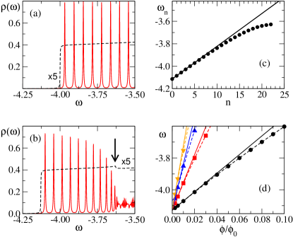
Figure 1: (color online) Density of states $\rho(\omega)$ vs. energy $\omega$, for (a) $\lambda=0$ and (b) $\lambda=0.2$. Dashed lines are for $B=0$ (times 5, for visibility), and full lines for $\phi/\phi_{0}=0.005$. The arrow in (b) marks the edge of the polaron+one phonon continuum. (c) Energies $\omega_{n}$ of the Landau levels vs. $n$ for $\phi/\phi_{0}=0.0025,\lambda=0.2$. The solid line is the prediction of Eq. (6); (d) The energy of the four lowest Landau levels as a function of $\phi/\phi_{0}$ for $\lambda=0.2$. The lines are the predictions of Eq. (6). Other parameters are $t=1,\Omega=0.5,\eta=0.002$.

Results: We begin with a weak field and weak electron-boson coupling, where we can compare with known perturbational results Sarma . In Fig. 1(a) we plot the DOS with/without (full/dashed line) a very small field $\phi/\phi_{0}=0.005$, in the absence of electron-boson coupling $\lambda=0$. The $B=0$ DOS is increased 5-fold for ease of view. As expected, it has a sharp rise at $-4t$ and then increases slowly. For $B\neq 0$, we see the Landau levels as a succession of Lorentzian peaks with width defined by $\eta$.

Fig. 1(b) shows the DOS at a weak coupling $\lambda=0.2$. The $B=0$ band-edge has moved below $-4t$, due to the formation of the polaron band. The top of the polaron band and the jump marking the edge of the polaron+one-boson continuum at $E_{GS}+\Omega$ are clearly visible (arrow). For $B\neq 0$, the polaron band splits into LLs with smaller spacing. Fig. 1(c) shows their energies $\omega_{n}$ when $\phi/\phi_{0}=0.0025$. The line shows the perturbational prediction:

$$\hbar\omega_{n}=E_{GS}+\hbar\omega_{c}^{*}\left(n+{1\over 2}\right)$$ (6)

where $\omega_{c}^{*}=eB/m^{*}$ is the cyclotron frequency, and we used the $B=0$ value of polaron effective mass, $m^{*}$ and of $E_{GS}$. (Here, $E_{GS}=-4.1288t$ and $m^{*}/m=1.0765$). At low energies the agreement is very good, but it worsens as the LLs approach the continuum. Note that as expected, as the spacings decrease near the top of the polaron band, so does the spectral weight in each LL. Even for low LLs, the agreement is worse at larger $B$, as shown in Fig. 1(d). The solid lines are Eq. (6) using again $m^{*}$. The dashed lines show fits using a $m^{*}(B)=m^{*}(1+\gamma B)$, a correction to the polaron effective mass predicted by perturbation theory Sarma . The agreement is much better although $\gamma$ increases with $n$, it is not a constant. Nevertheless, we conclude that at low-energies the agreement with perturbation theory predictions is good note .

At higher energies, however, it is not. Fig. 1(b) shows very different DOS in the continuum than below it. The failure of perturbation theory here is not surprising. Refs. Sarma use the free electron part as the large component, while electron+one-boson states are the small perturbation in the wavefunction. This is an accurate description at low energies but it fails at the top of the polaron band and inside the continuum, where the electron+one-boson states are dominant (for small $\lambda$) while the free electron part is small. This failure of non-degenerate perturbation theory at these higher energies is well known for $B=0$ models, see for example Fig. 4 of Ref. Nik .

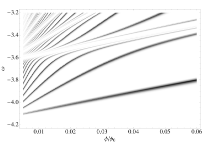
Figure 2: Contour plot of the density of states $\rho(\omega)$ vs $\omega$ and $\phi/\phi_{0}\in[0.005,0.06]$, for $\lambda=0.2$, $t=1,\Omega=0.5,\eta=0.005$.

What happens at these higher energies and also higher fields is shown in Fig. 2: the polaron LLs move to higher energies as $B$ increases, until reaching an avoided crossing at an energy defined by the continuum band-edge as $B\rightarrow 0$, and which also moves higher with $B$. Above it, we see a whole sequence of such avoided crossings at energies that increase faster and faster with increasing $B$.

The reason for this beautiful spectrum is easy to find. As mentioned, the $B=0$ polaron+one-boson continuum is due to excited states with a boson far from the polaron. At finite $B$, the continuum splits in a set of excited discrete states of energy $\hbar\omega_{n}+\Omega$, each with a boson far from the polaron in a LL state. The DOS weights the spectrum with the overlap with a free particle (zero bosons) state, see Eq. (2), so it vanishes at these energies. This explains the sequence of avoided crossings that occur at energies $\Omega$ above that of the low-energy LLs.

To our knowledge, this is the first time that this complex pattern is revealed. Perturbation theory Sarma predicts an avoided crossing at $\hbar\omega_{c}\approx\Omega$, i.e. at $\phi/\phi_{0}\approx 0.04$ for the values of Fig. 2. This is wrong but not surprising since as mentioned, non-degenerate perturbation theory is no longer valid at these energies. Perturbation theory also makes predictions about high fields $\hbar\omega_{c}\gg\Omega$. Here, Hofstadter butterfly effects become important for our model (they are absent in Refs. Sarma which use continuous models). For small $\lambda$, the DOS is quite complex because of overlap with the continuum and higher energy features. The results will be discussed elsewhere.

Instead, here we focus on another interesting question, namely how like a particle is a strongly dressed quasiparticle? To answer this, we look at the Hofstadter spectrum of a small polaron, for $\lambda>1$. As is well-known, at $B=0$ the small polaron band flattens considerably and a gap opens between it and the higher-energy features Holger ; MA . This gap allows us to look at the polaron response alone, avoiding overlap with these higher energy features.

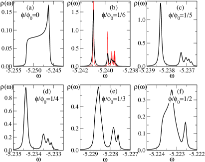
Figure 3: (color online) Density of states $\rho(\omega)$ vs. energy $\omega$, for $\lambda=1.2$, $t=1$, $\Omega=0.5$ and various magnetic fluxes $\phi/\phi_{0}$. The thick black lines correspond to $\eta=5\cdot 10^{-5}$, while the thin red line in panel (b) is for $\eta=10^{-5}$. The polaron band shows the Hofstadter signature, splitting into $q$ sub-bands if $\phi/\phi_{0}=p/q$. Higher energy features are not shown.

Fig. 3 shows results for $\lambda=1.2$, a value just above the crossover into the small polaron regime Holger ; MA . Panel (a) is the polaron band DOS at $B=0$. The GS energy is significantly lower because of the much larger binding energy, and the bandwidth is very narrow because of the large effective mass $m^{*}$. As mentioned, this band is now separated by a gap from higher energy features.

Panels (b)-(f) show the low-energy DOS for a magnetic flux $\phi/\phi_{0}=1/6\rightarrow 1/2$. The $B=0$ band indeed splits into $q$ subbands for $\phi/\phi_{0}=p/q$, as expected for a bare particle. For larger $q$ the subbands become narrower and a smaller $\eta$ is needed. In panel (b) the thin line shows the DOS for $\eta\rightarrow\eta/5$. The peaks increase much less than 5 times, proving that these are true continua (although very narrow and thus not yet fully converged at this $\eta$), not discrete Lorentzians. For smaller $q$ the subbands become much wider than $\eta$ and are already converged.

We have checked (not shown) that, as required, spectra are unchanged if $\phi/\phi_{0}\rightarrow 1\pm\phi/\phi_{0}$. We also see that $E_{GS}(B)$ increases significantly with $\phi/\phi_{0}$, reaching its maximum at $\phi/\phi_{0}=1/2$, consistent with the Hofstadter spectrum of a particle on a square lattice Hofs . However, there are also big differences. The polaron spectra are asymmetric: the lowest subband has most of the weight and is quite distinct from the other subbands. This is very unlike the Hofstadter spectrum of the bare particle on a square lattice, which has particle-hole symmetry.

This symmetry is lost even at $B=0$, where the DOS is not symmetric about the center of the band. The reason (see Fig. 4) is that while the van-Hove singularity is still due to the flat $E(\mathbf{k})$ along the $(0,\pi)-(\pi,0)$ line, it is now located just below the upper band edge. Moreover, as shown in panel (b), the quasiparticle weight is $\sim$ 2 orders of magnitude smaller here than near $\mathbf{k}=0$. Taken together, these explain the skewed shape of the $B=0$ DOS. They also show that nn hopping with a $t^{*}/t=m/m^{*}=\exp(-g^{2}/\Omega^{2})$ as predicted by first order, strong-coupling perturbation theory Bayo , is not enough to fit $E(\mathbf{k})$, even though $m^{*}/m\approx 91$. Second order perturbation adds second and third nn hopping Bayo :

$$t_{2}^{*}=2t_{3}^{*}=-2{t^{2}\over\Omega}e^{-2{g^{2}\over\Omega^{2}}}\sum_{n=1}^{\infty}{1\over nn!}\left({g\over\Omega}\right)^{2n}$$

which also give a poor fit, with non-monotonic behavior along all cuts shown in Fig. 4, except the $(0,\pi)-(\pi,0)$ line whose flatness is preserved. Indeed, to reasonably fit $E(\mathbf{k})$ one needs to add $\cos(nk_{x}a+mk_{y}a)$ terms with up to $|n|+|m|\approx 6$. In other words, one needs to include terms at least up to 6th order in perturbation theory in the hopping Hamiltonian to properly describe it.

Figure 4: Polaron energy $E(\mathbf{k})$ (top) and quasiparticle weight $Z(\mathbf{k})$ (bottom) vs $\mathbf{k}$, for $B=0,t=1,\Omega=0.5,\lambda=1.2$.

The long range hopping in $E(\mathbf{k})$ and the varying $Z(\mathbf{k})$ explain the asymmetry of the polaron Hofstadter spectra. Taken together with the low-$\lambda$ results, they also show that a polaron is not behaving just like a bare heavier particle with mass $m^{*}$. Instead, its composite structure and the existence of higher energy states signal their existence in its finite-$B$ response. This has obvious implications for the interpretation of experimental data.

Acknowledgements: Work supported by NSERC and CIFAR. We thank P. Stamp for suggesting the problem, and H. Fehske and G. Sawatzky for discussions.

References

- (1) For a review, see H. Fehske and S. A. Trugman, in Polarons in Advanced Materials, edited by A. S. Alexandrov (Springer-Verlag, Dordrecht, 2007).
- (2) M. Berciu, Phys. Rev. Lett. 97, 036402 (2006); G. L. Goodvin et al, Phys. Rev. B 74, 245104 (2006); M. Berciu and G. L. Goodvin, Phys. Rev. B 76, 165109 (2007).
- (3) G. L. Goodvin and M. Berciu, Phys. Rev. B 78 235120 (2008); L. Covaci and M. Berciu, Phys. Rev. Lett. 102, 186403 (2009); M. Berciu and H. Fehske, Phys. Rev. B 82, 085116 (2010).
- (4) S. Das Sarma, Phys. Rev. Lett. 52, 859 (1984); R. Chen et al, Phys. Rev. B 41, 1435 (1990); F. M. Peeters et al, Phys. Rev. B 45, 4296 (1992); G. Q. Hai et al, Phys. Rev. B 47, 10358 (1993); D. E. N. Brancus and G. Stan, Phys. Rev. B 63, 235203 (2001); Y. Chen et al, Phys. Rev. B 79, 235314 (2009).
- (5) D. R. Hofstadter, Phys. Rev. B 14, 2239 (1976).
- (6) T. Holstein, Ann. Phys. (N.Y.) 8, 325 (1959).
- (7) G. L. Goodvin, L. Covaci and M. Berciu, Phys. Rev. Lett. 103, 176402 (2009); M. Berciu et al, Europhys. Lett. 89, 37007 (2010).
- (8) O. S. Baris̃ić, Phys. Rev. Lett. 98, 209701 (2007); M. Berciu, Phys. Rev. Lett. 98, 209702 (2007).
- (9) M. Berciu and A. M. Cook, unpublished.
- (10) The work in Refs. Sarma is for the Fröhlich parabolic model, however except for changed coefficients one expects similar results for the Holstein model at low energies.
- (11) N. V. Prokof’ev and B. V. Svistunov, Phys. Rev. Lett. 81, 2514 (1998).
- (12) B. Lau et al, Phys. Rev. B 76, 174305 (2007); F. Marsiglio, Physica C 244, 21 (1995).