Effects of Varying the Three-Body Molecular Hydrogen Formation Rate in Primordial Star Formation

Abstract

The transformation of atomic hydrogen to molecular hydrogen through three-body reactions is a crucial stage in the collapse of primordial, metal-free halos, where the first generation of stars (Population III stars) in the Universe are formed. However, in the published literature, the rate coefficient for this reaction is uncertain by nearly an order of magnitude. We report on the results of both adaptive mesh refinement (AMR) and smoothed particle hydrodynamics (SPH) simulations of the collapse of metal-free halos as a function of the value of this rate coefficient. For each simulation method, we have simulated a single halo three times, using three different values of the rate coefficient. We find that while variation between halo realizations may be greater than that caused by the three-body rate coefficient being used, both the accretion physics onto Population III protostars as well as the long-term stability of the disk and any potential fragmentation may depend strongly on this rate coefficient.

1 Introduction

To constrain the initial mass of the first stars in the Universe, the so-called Population III stars, we need to be able to understand and model the gravitational collapse of the progenitor clouds that give birth to them. The physics of this collapse is governed in large part by the thermal evolution of the gas (see e.g. Bromm & Larson, 2004; Glover, 2005). In primordial, metal-free gas, this is regulated by cooling from molecular hydrogen ($\mathrm{H}_{2}$), as has been known since Saslaw & Zipoy (1967) first constructed analytical estimates for the importance of molecular hydrogen cooling in pre-galactic clouds. Early studies of the formation of molecular hydrogen in protogalaxies focussed on its formation by ion-neutral reactions at low densities (Saslaw & Zipoy, 1967; Peebles & Dicke, 1968; Matsuda et al., 1969). In this regime, the dominant formation pathway has been shown to be the electron-catalyzed pair of reactions

$$\mathrm{H}+\mathrm{e}^{-} \rightarrow \mathrm{H}^{-}+\gamma$$ (1)

$$\mathrm{H}^{-}+\mathrm{H} \rightarrow \mathrm{H}_{2}+\mathrm{e}^{-}.$$ (2)

The rate-limiting step in this pair of reactions is generally the formation of the $\mathrm{H}^{-}$ ion, and the rate coefficient for this reaction is known very accurately (Galli & Palla, 1998). The rate coefficient for the second reaction, the associative detachment of the $\mathrm{H}^{-}$ ion to form $\mathrm{H}_{2}$, is more uncertain, and in some circumstances, this uncertainty can significantly affect the time taken for the primordial gas to undergo gravitational collapse and the minimum temperature reached during the collapse (Glover et al., 2006; Glover & Abel, 2008). However, recent experimental work (Kreckel et al., 2010) has reduced this uncertainty to a level at which it is unlikely to significantly affect the results of future calculations.

This rate at which $\mathrm{H}_{2}$ can be formed by reactions 1 and 2 depends on the free electron abundance. As primordial gas collapses, recombination causes it to decline, with the result that further $\mathrm{H}_{2}$ formation soon becomes very difficult. By comparing the timescales for $\mathrm{H}_{2}$ formation and $\mathrm{H}^{+}$ recombination, it is simple to show that the asymptotic fractional abundance of $\mathrm{H}_{2}$ should be of order $10^{-3}$ (see e.g. Susa et al., 1998), an estimate that has since been confirmed in numerous numerical simulations (see e.g. Abel et al. (2002), hereafter ABN02, and Bromm et al. (2002); Yoshida et al. (2003)). However, this is not the end of the story. At high densities, Palla et al. (1983) (hereafter PSS83) showed that three-body processes would come to dominate the formation of $\mathrm{H}_{2}$. A number of different three-body reactions are possible (see the discussion in Glover & Savin, 2009), but the dominant reaction involves atomic hydrogen as the third body:

$$\mathrm{H}+\mathrm{H}+\mathrm{H}\rightarrow\mathrm{H}_{2}+\mathrm{H}.$$ (3)

This reaction has a very small rate coefficient, but the rate at which $\mathrm{H}_{2}$ is formed by this process increases rapidly with increasing density. Therefore, at high densities this reaction is able to rapidly convert most of the hydrogen in the gas from atomic to molecular form.

The published rate coefficients for reaction 3 were surveyed by Glover (2008), who showed that although most of the published values agreed reasonably well at high temperatures, they disagreed by orders of magnitude at the lower temperatures relevant for $\mathrm{H}_{2}$ formation in primordial gas. Since $\mathrm{H}_{2}$ is the dominant coolant in primordial gas, it is reasonable to suppose that a large uncertainty in its formation rate at high densities may lead to a large uncertainty in the thermal evolution of this dense gas. Moreover, the situation is further exacerbated by the fact that each time an $\mathrm{H}_{2}$ molecule is formed via reaction 3, $4.48~{}\mathrm{eV}$ of energy is released, corresponding to the binding energy of the molecule, with almost all of this energy subsequently being converted into heat. There is thus a substantial chemical heating rate associated with the three-body formation of $\mathrm{H}_{2}$, and at the densities at which reaction 3 is most important, this can become the dominant source of heat in the gas.

The influence of the uncertainty in the rate coefficient for reaction 3 was studied in Glover & Abel (2008) and Glover & Savin (2009), who confirm that it introduces significant uncertainty into the thermal evolution of the gas at densities $\rho>10^{-16}~{}\mathrm{g}~{}\mathrm{cm}^{-3}$. However, both of these studies involved the use of highly simplified one-zone models for the gas, in which the gas was assumed to collapse as if in free-fall, with changes in the temperature having no effect on the dynamical behaviour.

In this paper, we present the results of a study that uses high-resolution, high dynamical range hydrodynamical simulations of Population III star formation to examine the impact that the uncertainty in the rate coefficient for reaction 3 has on both the thermal and the dynamical evolution of the gas, in order to determine whether this uncertainty will be an important limitation on our ability to make predictions of the Population III initial mass function. In order to ensure that our results are not unduly influenced by our choice of numerical method, we perform simulations using two very different hydrodynamical codes: the Enzo adaptive mesh refinement (AMR) code, and the Gadget smooth particle hydrodynamics (SPH) code. Although these codes have been compared in past studies (O’Shea et al., 2005; Regan et al., 2007), this is the first time that they have been directly compared in a study of Population III star formation.

The structure of our paper is as follows: first we describe the setup and chemical model for our simulations in Section 2; in Section 3 we describe the results of our calculations; in Section 4 we discuss these results and their interplay with the molecular hydrogen three-body rates; and finally we conclude with a summary of our findings and a suggestion for a three-body rate to standardize on in Section 5.

2 Simulations

2.1 Three-Body Rates

$\mathrm{H}_{2}$ Formation Rates ($\mathrm{cm}^{6}~{}\mathrm{s}^{-1}$)
ABN02	$1.3\times 10^{-32}(T/300)^{-0.38}\hskip 21.68121pt(T<300~{}\mathrm{K})$
ABN02	$1.3\times 10^{-32}(T/300)^{-1.00}\hskip 21.68121pt(T>300~{}\mathrm{K})$
PSS83	$5.5\times 10^{-29}/T$
FH07	$1.44\times 10^{-26}/T^{1.54}$
$\mathrm{H}_{2}$ Destruction Rates ($\mathrm{cm}^{3}~{}\mathrm{s}^{-1}$)
ABN02	$(1.0670825\times 10^{-10}\times(T_{\mathrm{eV}})^{2.012})/(\exp(4.463/T_{\mathrm{eV}})\times(1+0.2472T_{\mathrm{eV}})^{3.512})$
PSS83	$5.24\times 10^{-7}\times T^{-0.485}\exp(-52000/T)$
FH07	$1.38\times 10^{-4}\times T^{-1.025}\exp(-52000/T)$

Table 1: Formation and destruction rates for all three studied sets of rates. $T$ is the gas temperature in Kelvin and $T_{\mathrm{eV}}$ is defined as $T/11605$ (the temperature in units of eV).

.

The three-body rates we chose to compare in this study were taken from ABN02, PSS83, and Flower & Harris (2007) (hereafter FH07); their values as a function of temperature are shown in Figure 1. We have tabulated these rates in Table 1. The ABN02 rate is based on the theoretical calculations of Orel (1987) at low temperatures ($T<300\>{\rm K}$). At higher temperatures, Abel et al. assumed, in the absence of better information, that the rate was inversely proportional to temperature. This choice means that the Abel et al. rate has a sudden change of slope at $T=300\>{\rm K}$, which is somewhat artificial. However, in practice this feature appears to be harmless for Population III.1 star formation, as in previous simulations of collapsing primordial gas clouds, the gas was always significantly hotter than 300 K by the time the gas density reached the domain in which three-body $\mathrm{H}_{2}$ formation dominates. For subsequent Population III.2 star formation, where $\mathrm{HD}$cooling may dominate, this feature may indeed be important (Yoshida et al., 2007). The AMR and SPH calculations utilized different dissociation rates for the ABN02 calculations, which have been plotted separately; the AMR calculation utilized a density-dependent match to the rate given in Martin et al. (1996), whereas the SPH calculation utilized a temperature-dependent value calculated via the principle of detailed balanced. We have plotted the ABN02A rate at a density of $\mathrm{n}_{\mathrm{H}}=10^{9}~{}\mathrm{cm}^{-3}$. The rates from PSS83 and FH07 were both computed using the principle of detailed balance, applied to the two-body collisional dissociation reaction

$$\mathrm{H}_{2}+\mathrm{H}\rightarrow\mathrm{H}+\mathrm{H}+\mathrm{H}.$$ (4)

The two studies obtained different three-body rates from this procedure on account of the different assumptions they made regarding the temperature dependence of the $\mathrm{H}_{2}$ partition function (Flower & Harris, 2007). In all three cases, we ensured that the $\mathrm{H}_{2}$ collisional dissociation rate used in the simulations was consistent with the chosen three-body $\mathrm{H}_{2}$ formation rate. We know that for a system in chemical and thermal equilibrium, the rate at which H₂ is produced by reaction 3 must equal the rate at which it is destroyed by reaction 4; this is a simple consequence of the principle of microscopic reversibility (see e.g. Denbigh 1981 for a detailed discussion). We also know that for a system in chemical and thermal equilibrium, the ratio of the equilibrium abundances of atomic and molecular hydrogen are related by the Saha equation

$$\frac{n_{\rm H_{2}}}{n_{\rm H}^{2}}=\frac{z_{\rm H_{2}}}{z_{\rm H}^{2}}\left(\frac{h^{2}}{\pi m_{\rm H}kT}\right)^{3/2}\exp\left(\frac{E_{\rm diss}}{kT}\right),$$ (5)

where $n_{\rm H_{2}}$ and $n_{\rm H}$ are the number densities of H₂ and atomic hydrogen, respectively, $z_{\rm H_{2}}$ and $z_{\rm H}$ are the partition functions of H₂ and atomic hydrogen, $E_{\rm diss}$ is the dissociation energy of H₂ and the other symbols have their usual meanings. Now, since $k_{\rm f}/k_{\rm r}=n_{\rm H_{2}}/n_{\rm H}^{2}$, where $k_{f}$ is the rate coefficient for reaction 3 and $k_{r}$ is the rate coefficient for reaction 4, this implies that

$$\frac{k_{\rm f}}{k_{\rm r}}=\frac{z_{\rm H_{2}}}{z_{\rm H}^{2}}\left(\frac{h^{2}}{\pi m_{\rm H}kT}\right)^{3/2}\exp\left(\frac{E_{\rm diss}}{kT}\right),$$ (6)

provided that the gas in is local thermodynamic equilibrium (LTE), which is a reasonable approximation at the densities and temperatures for which three-body H₂ formation is an important process. Therefore, if we change the three-body H₂ formation rate coefficient, we must also change the rate coefficient for $\mathrm{H}_{2}$ collisional dissociation (in the LTE limit) in such a fashion that Equation 6 remains satisfied.

Two additional rates discussed in Glover (2008) – one that was derived there for the first time, and another that was suggested by Cohen & Westberg (1983) – are not included in our study. In common with the PSS83 rate, these rates lie between the extremes represented by the ABN02 and FH07 rates, and so we would expect them to yield behaviour similar to that we find for the PSS83 rate.

Finally, we note that in this study we do not investigate the effects of any uncertainties in the rate coefficients of other three-body reactions, such as

$${\rm H}+{\rm H}+{\rm He}\rightarrow{\rm H_{2}}+{\rm He}.$$ (7)

This process is included in the chemical network used for our SPH simulations, along with its inverse

$${\rm H_{2}}+{\rm He}\rightarrow{\rm H}+{\rm H}+{\rm He},$$ (8)

but in practice their effects are unimportant, as these reactions are never responsible for more than a few percent of the total H₂ formation or destruction rate (see e.g. Glover & Savin 2009). These reactions are not included in the chemical network used for our AMR simulations, but in view of their unimportance, we do not expect this difference in the chemical networks to significantly affect our results.

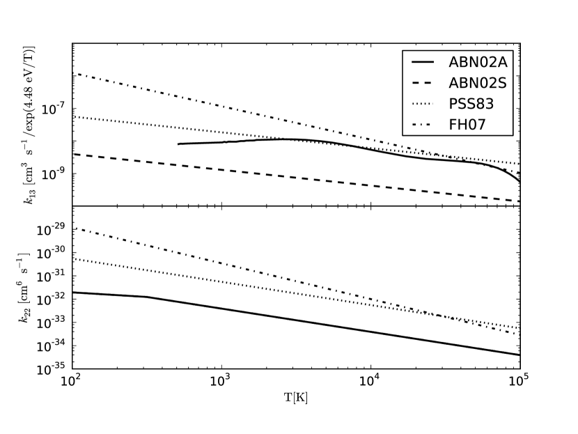
Figure 1: Collisional dissociation (top) and three-body association (bottom) rates from ABN02 (solid: simulation ABN02A, dashed: ABN02S), PSS83 (dotted: simulations PSS83A & PSS83S), and FH07 (dash-dot: simulations FH07A & FH07S). A factor of $\exp{4.48~{}\mathrm{eV}/\mathrm{T}}$ has been divided out of the collisional dissociation rate, for clarity. We note that the solid and dashed lines, for simulations ABN02A and ABN02S, are coincident in the lower panel.

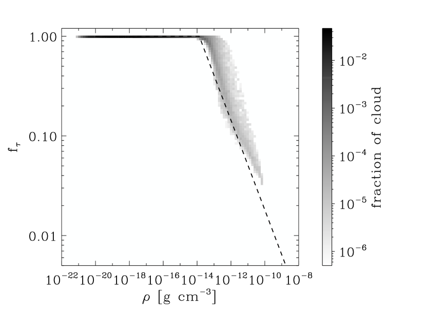
Figure 2: Comparison of the optical depth approximations for the SPH calculations (phase diagram) versus the AMR calculations (solid black line). $f_{\tau}$ is the ratio between the optically thick and optically thin cooling rates. The left-hand panel compares the two approximations at the time at which the peak density was $7.9\times 10^{-11}\mathrm{g}~{}\mathrm{cm}^{-3}$, while the right-hand panel shows the comparison at a later time, when the peak density was $2.7\times 10^{-9}\mathrm{g}~{}\mathrm{cm}^{-3}$.

2.2 Simulation Setup

For each of our selected three-body rates, we perform two simulations, one using an adaptive mesh refinement (AMR) code, and a second one using a smoothed particle hydrodynamics (SPH) code. As well as utilizing different computational approaches, these two sets of simulations also use slightly different initial conditions, as described below, although in both cases the simulations probe what are typical conditions for the formation of Population III stars. Our rationale for this dual approach is to be able to demonstrate that the uncertainty introduced into the outcome of the simulations by our poor state of knowledge regarding the rate of reaction 3 is largely independent of our choice of initial conditions or numerical method. In the following subsections, we describe in more detail the setups used for our AMR and SPH simulations (sections 2.2.1 and 2.2.2, respectively), and also briefly discuss the different approaches that we use to treat $\mathrm{H}_{2}$ cooling in the optically thick limit (section 2.2.3).

2.2.1 Adaptive mesh refinement simulations

Simulations ABN02A, PSS83A and FH07A were conducted using the adaptive mesh refinement code Enzo, a three-dimensional cosmological adaptive mesh refinement code written by Greg Bryan, with ongoing development at many institutions, including the Laboratory for Computational Astrophysics (UCSD), Stanford University, and Columbia University. Enzo includes physical models for radiative cooling, non-equilibrium primordial chemistry, $N$-body dark matter and hydrodynamics (O’Shea et al. 2004; Bryan et al. 2001; Bryan & Norman 1997, data analysis using yt, Turk et al. 2010b). Here, we use a coupled chemistry and cooling solver, including the $4.48\mathrm{eV}$ energy deposition and removal for each molecule of hydrogen. Each simulation uses a single set of rate coefficients, as noted in Figure 1. ABN02A uses the rates taken from ABN02, PSS83A from PSS83, and FH07A from FH07.

Simulations ABN02A, PSS83A, and FH07A were initialized at $z=99$ assuming a concordance $\Lambda$ cold dark matter ($\Lambda$CDM) cosmological model: total matter density $\Omega_{\mbox{\tiny{m}}}=0.27$, baryon density $\Omega_{\mbox{\tiny{b}}}=0.0463$, dark matter density $\Omega_{\mbox{\tiny{CDM}}}=0.2237$, dark energy density $\Omega_{\Lambda}=0.73$, Hubble parameter $h=H_{0}/100~{}{\rm km}~{}{\rm s}^{-1}~{}{\rm Mpc}^{-1}=0.72$, where $H_{0}$ is the Hubble expansion rate today, spectral index $n_{s}=1.0$, and power spectrum normalization $\sigma_{8}=0.7$ (Spergel et al., 2007). However, while the specific cosmological parameters govern the halo itself, we intend to compare the hydrodynamical and chemical state of the gas across realizations while varying the formation and dissociation rate of molecular hydrogen; the results should be largely immune to small variations in the cosmology used. A random cosmological realization is used, with a box size of $0.3h^{-1}$ Mpc (comoving), centered on the location of the earliest collapsing massive halo, of mass $5\times 10^{5}~{}\mbox{M}_{\odot}$. We use recursive refinement to generate higher-resolution subgrids, with an effective resolution of $1024^{3}$ in the region of collapse. The most massive halo collapses at $z=17.1$, and we halt each of the four simulations when the maximum number density is $10^{16}~{}\mathrm{cm}^{-3}$, corresponding to a mass density slightly greater than $10^{-8}~{}\mathrm{g}~{}\mathrm{cm}^{-3}$.

2.2.2 Smoothed particle hydrodynamics simulations

Simulations ABN02S, PSS83S and FH07S were conducted using the Gadget 2 smoothed particle hydrodynamics code (Springel, 2005). We have modified the publicly available version of Gadget 2 to add a treatment of primordial gas chemistry and cooling, discussed in detail elsewhere (Glover & Jappsen, 2007; Clark et al., 2010). As with the AMR simulations, each of our SPH simulations uses a single set of rate coefficients, taken from ABN02, PSS83 and Flower & Harris (2007), respectively.

The SPH simulations differ from the AMR in that they are run in two distinct stages. First, we model the formation of the minihalo in a cosmological simulation. We choose a side length of $200~{}{\rm kpc}$ (comoving) and initialize the parent simulation at $z=99$ with a fluctuation power spectrum determined by a concordance $\Lambda$CDM cosmology with $\Omega_{m}=0.3$, $\Omega_{b}=0.04$, $h=0.7$, $n_{s}=1.0$, and $\sigma_{8}=0.9$ (Spergel et al., 2003). In a preliminary run with $128^{3}$ dark matter particles and $128^{3}$ gas particles, we locate the formation site of the first minihalo that collapses and cools to high densities. We then re-initialize the simulation with three consecutive levels of refinement, replacing a parent particle by a total of $512$ daughter particles. To avoid the propagation of numerical artifacts caused by the interaction of particles of different masses, we choose the highest resolution region to have a side length of $50~{}{\rm kpc}$, which is much larger than the comoving volume of the minihalo. The particle mass within this region is $\simeq 0.26~{}\rm{M}_{\odot}$ in DM and $\simeq 0.04~{}{\rm M}_{\odot}$ in gas.

The cosmological simulation is then evolved until the gas in the minihalo has reached a density of $\rho=10^{-18}\>\mathrm{g}\>\mathrm{cm}^{-3}$, by which point the gas has gravitationally decoupled from its parent minihalo and has begun to collapse in its own right. At this point we discard the full cosmological simulation and focus our calculation on the central collapsing region and its immediate surroundings. These then become the initial conditions for our study of the three-body formation rates. The initial gravitational instability that leads to the collapse in the baryons occurs at around $\rho\sim 10^{-20}~{}\mathrm{g}~{}\mathrm{cm}^{-3}$ and $T\sim 270$ K, which corresponds to a Jeans mass of around 350 $\mbox{M}_{\odot}$. To ensure that we capture the entire collapsing fragment in our simulations, and to avoid any unphysical boundary effects, we select a spherical region containing 1000 $\mbox{M}_{\odot}$. To account for the effects of the missing gas that should surround our central core, we include a external pressure (Benz, 1990) that modifies the standard gas-pressure contribution to the Gadget2 momentum equation,

$$\frac{dv_{i}}{dt}=-\sum_{j}m_{j}\left[f_{i}\frac{P_{i}}{\rho_{i}^{2}}\nabla_{i}W_{ij}(h_{i})+f_{j}\frac{P_{j}}{\rho_{j}^{2}}\nabla_{i}W_{ij}(h_{j})\right],$$ (9)

by replacing $P_{i}$ and $P_{j}$ with $P_{i}-P_{\rm ext}$ and $P_{j}-P_{\rm ext}$ respectively, where $P_{\rm ext}$ is the external pressure, and all quantities have the usual meaning, consistent with those used by Springel (2005). The pair-wise nature of the force summation over the SPH neighbors ensures that $P_{\rm ext}$ cancels for particles that are surrounded by other particles. Only at the edge does the term not disappear, where it mimics the pressure contribution from the surrounding medium. The average density and temperature at the edge of our $1000~{}\mbox{M}_{\odot}$ cloud are $10^{-20}~{}\mathrm{g}~{}\mathrm{cm}^{-3}$ and 270 K respectively. These average values are used to define the value of $P_{\rm ext}$.

To evolve the collapse of the gas to high densities, we also need to increase the resolution. Since the SPH particle mass in the original cosmological simulation was $0.04~{}\mbox{M}_{\odot}$, our selected region contains only $\sim 20,000$ SPH particles. To increase the resolution, we ‘split’ the particles into 100 SPH particles of lower mass. This is done by randomly placing the sibling particles inside the smoothing length of parent particle. Apart from the mass of the siblings, which is 100 times less that of the parent, they inherit the same values for the entropy, velocities and chemical abundances as their parents.

Although this set-up permits us to follow the evolution of the baryons over many orders of magnitude in density, the SPH calculations in this study do not achieve the same resolution as the AMR calculations. The initial Jeans-unstable region in the SPH calculations is resolved by roughly 9,000 particles, or $\sim 20^{3}$. In contrast, the AMR calculations are set to resolve the Jeans length by $16^{3}$ grid cells, at all times. As such, they can much better resolve the turbulence and structure that develops during the collapse of the baryons. Along with the slightly higher degree of rotation found in the minihalo modelled in the SPH calculations, this explains why the SPH calculation contain significantly less density structure than the AMR simulations. This will be discussed further in Section 3.

2.2.3 Molecular hydrogen cooling in optically thick gas

The two different codes utilized different mechanisms for treating $\mathrm{H}_{2}$ cooling at high densities ($\rho\geq 10^{-14}\mathrm{g}~{}\mathrm{cm}^{-3}$), in the regime where the lines become optically thick. In the AMR simulations, we used the approximation proposed by Ripamonti & Abel (2004), which provides a functional form dependent only on density, initially calculated in that work via escape fraction estimates and then calibrated to 1D simulation results. In the SPH simulations, we used the classic Sobolev approximation, as implemented in Yoshida et al. (2006), where the local density and velocity gradient are used to compute an optical depth correction independently for each gas particle. In Figure 2, we compare the effective suppression of ro-vibrational cooling produced by these two approaches at two different times during the collapse, using data from run ABN02S to construct the optical depth correction factors for the Sobolev approach. We note that while the two approximations are in general agreement, the Ripamonti & Abel (2004) approximation generally suppresses cooling slightly more than the Sobolev-based approximation, albeit with a sharper turn-on point. Comparison of the left and right-hand panels in Figure 2 demonstrates that the differences between the two methods do not appear to depend strongly on the time at which the comparison is made, although it is plausible that we would find greater differences were we to examine much later times in the evolution of the system, after the formation of the initial protostar. The differences between the two methods for suppressing ro-vibrational cooling may affect the temperature of the two simulations, but as they are typically not larger than a factor of two, we believe that this effect will be secondary to the variance in the physical conditions between the two halos.

3 Results

Except where otherwise indicated, we have compared the two sets of simulations at the time when their peak density was $10^{-8}~{}\mathrm{g}~{}\mathrm{cm}^{-3}$. Ideally, these simulations would be compared at epochs of relative time between collapses and transitions between physical processes; however, owing to the difference in halos, the difference in collapse time (§ 3.1) and pragmatic issues of coordinating two different simulation methodologies and two different halos, we have instead chosen to compare the six simulations at identical peak densities.

3.1 Collapse Time

We first investigated the time taken to reach a density of $10^{-8}~{}\mathrm{g}~{}\mathrm{cm}^{-3}$ in the six simulations. To allow us to directly compare the final SPH simulations, which start with a central density of $3.4\times 10^{-18}\mathrm{g}~{}\mathrm{cm}^{-3}$, with the AMR simulations, which start from cosmological densities, we chose to measure the collapse times from the moment at which the maximum density in the simulation was $10^{-17}~{}\mathrm{g}~{}\mathrm{cm}^{-3}$. Once we had identified the most rapidly collapsing AMR and SPH simulations, we computed the time by which collapse was delayed in the more slowly collapsing simulations. These values are listed in Table 2. In both the SPH and the AMR simulations, the rate of collapse is directly related to the rate coefficient of the 3-body $\mathrm{H}_{2}$ formation, with the simulations employing the rate coefficient of Flower & Harris (2007) collapsing the fastest and those using the coefficient from ABN02 collapsing the slowest. For reference, the gravitational free-fall time of the gas with $\rho=10^{-17}~{}\mathrm{g}~{}\mathrm{cm}^{-3}$ was $t_{\mathrm{ff}}=\sqrt{3\pi/32G\rho}\simeq 21000\>\mathrm{yr}$. In addition, the free-fall times at densities of $10^{-16}~{}\mathrm{g}~{}\mathrm{cm}^{-3}$ and $10^{-10}~{}\mathrm{g}~{}\mathrm{cm}^{-3}$ – those over which the $\mathrm{H}_{2}$ formation takes place – are 6657 yr and 6.7 yr respectively. As such, the delays seen in the different simulations are long compared to the free fall times in the relevant stages of the collapse. This is particularly apparent in run ABN02A, where the collapse is delayed by almost seven free-fall times compared to run FH07A. Any delay in collapse time can have a profound implication on the incidence of fragmentation and the formation of multiple stars, as discussed in Section 4.

Simulation	$\Delta t\>[\mathrm{years}]$	Simulation	$\Delta t\>[\mathrm{years}]$
ABN02A	$135447$	ABN02S	$17908$
PSS83A	$6424$	PSS83S	$15978$
FH07A	$0$	FH07S	$0$

Table 2: Time required to collapse from $\rho_{\mathrm{max}}(t)=10^{-17}~{}\mathrm{g}~{}\mathrm{cm}^{-3}$ to $\rho_{\mathrm{max}}(t)=10^{-8}~{}\mathrm{g}~{}\mathrm{cm}^{-3}$, relative to the the time taken in the most rapidly collapsing simulation.

3.2 Radial Profiles

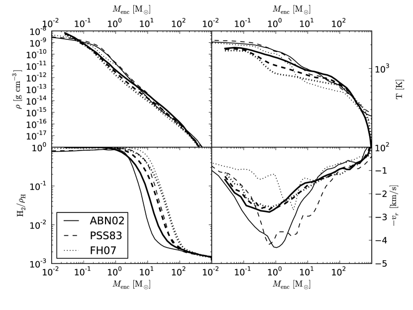
Figure 3: Radially-binned, spherically averaged profiles of density (volume-weighted, upper left), temperature (mass-weighted, upper right), molecular hydrogen mass-fraction (mass-weighted, lower left) and radial velocity (mass-weighted, lower right) plotted as a function of enclosed mass, measured from the densest point in the calculation. Thin lines correspond to the AMR simulations and thick lines correspond to the SPH simulations.

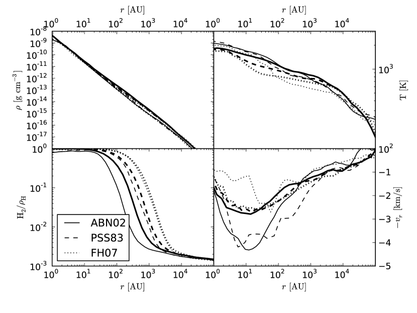
Figure 4: Radially-binned, spherically averaged profiles of density (volume-weighted, upper left), temperature (mass-weighted, upper right), molecular hydrogen mass-fraction (mass-weighted, lower left) and radial velocity (mass-weighted, lower right) plotted as a function of radius from the most dense point in the calculation. Thin lines correspond to the AMR simulations and thick lines correspond to the SPH simulations.

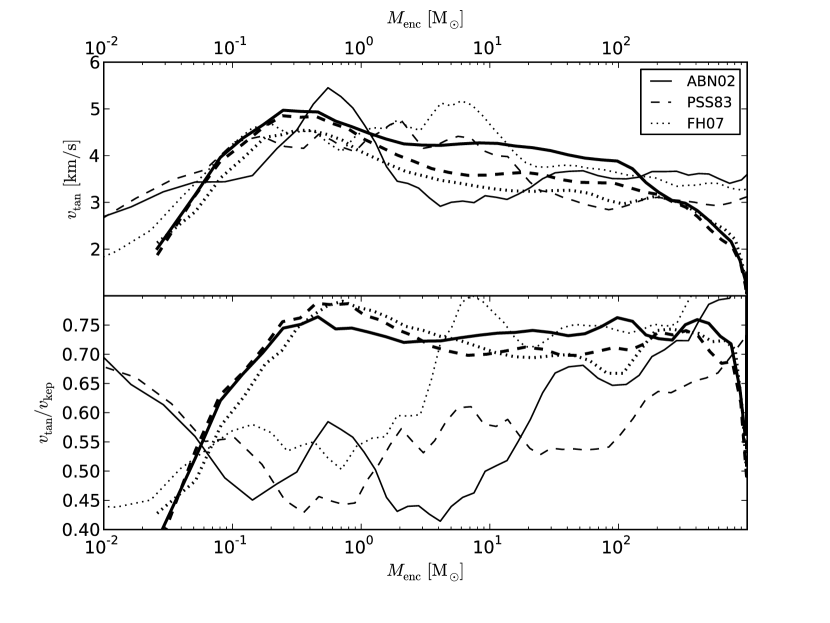
Figure 5: Radially-binned, spherically averaged profiles of tangential velocity (upper panel) and tangential velocity divided by Keplerian velocity (lower panel), plotted as a function of enclosed mass, measured from the densest point in the calculation. The velocity of the innermost bin has been subtracted prior to the calculation of the relative velocities. Thin lines correspond to the AMR simulations and thick lines correspond to the SPH simulations.

In Figure 3 we have plotted averaged spherical shell profiles of the six realizations, where the innermost bin is taken at the most dense point in the simulation and the values have been plotted as a function of the mass enclosed within each radial bin. In Figure 4, we have plotted the same spherically-averaged values as a function of the radius.

The upper left panels of Figures 3 and 4 show the volume-weighted average density, with the AMR results plotted in thin lines, and the SPH results in thick lines. In both sets of simulations, we see a similar dependence on the three-body reaction rate. The highest density at a given enclosed mass (or, alternatively, the highest enclosed mass at a given density) is produced by the ABN02 and PSS83 rates, which give very similar results. The FH07 rate produces systematically lower enclosed masses in both simulations, over a wide range in radii. The differences appear small, owing to the wide range of scales covered by the plot, but in the worst case can amount to a factor of two uncertainty in the enclosed mass (see e.g. $M_{\mathrm{enc}}$ in the three SPH simulations at a density $\rho=10^{-13}~{}\mathrm{g}~{}\mathrm{cm}^{-3}$). Nevertheless, the uncertainty introduced by the choice of three-body rate coefficient is less significant than the difference between the SPH and AMR realizations. For enclosed masses less than about 10 M_⊙, the SPH simulations are of characteristically lower density, indicating a core that is overall less massive. For example, the AMR simulations enclose roughly $0.5~{}\mbox{M}_{\odot}$ of gas that is of density $5\times 10^{-10}\mathrm{g}~{}\mathrm{cm}^{-3}$ or higher, whereas the SPH simulations enclose only $0.1~{}\mbox{M}_{\odot}$ in this density range. At enclosed masses greater than $\sim 5~{}\mbox{M}_{\odot}$, the two sets of simulations are in good agreement, and the radial profiles show extremely good agreement for all six realizations.

The upper right panels of Figures 3 and 4 show the mass-weighted average temperature, where the AMR simulations are plotted in thin lines and the SPH simulations are plotted in thick lines. Here we again see the same trend with rate coefficient in both sets of simulations: the ABN02 rate produces the hottest gas, and the FH07 rate the coldest. However, as before, the difference between the runs with different rate coefficients is comparable to the difference between the realizations. The AMR simulations produce a slightly hotter core than the SPH simulations, with a peak temperature of just over $2000~{}\mathrm{K}$ in the former, compared to $\sim 1700~{}\mathrm{K}$ in the latter. The AMR results for ABN02 and PSS83 show a more dramatic increase in the temperature at the onset of three-body molecular hydrogen formation than their counterpart SPH simulations, but outside of the central molecular region (the innermost $\sim 1-10~{}\mbox{M}_{\odot}$), both codes show good agreement. We note also that the radial temperature plots show better agreement to smaller scales; this is consistent with the overall larger protostellar core in the AMR simulations.

The lower left panels of Figures 3 and 4 show the mass-weighted average molecular hydrogen fraction, where the AMR simulations are plotted in thin lines and the SPH simulations are plotted in thick lines. Here, the difference between realizations is smaller than the uncertainty introduced by the choice of three-body rate coefficient. The physical size of the molecular cores in the AMR and SPH simulations agree very well for the FH07 and PSS83 rates, but disagree somewhat for the ABN02 rate, particularly for small $\mathrm{H}_{2}$ fractional abundances. This may be a consequence of the different dissociative rate, but that should largely be unchanged at the considered temperatures. Additionally, we note that the molecular core in the AMR calculations appears to be defined by a sharper contrast as a function of radius in the ABN02 run, a result of the lower dissociative rate in the ABN02A calculation. The divergence between the three rates in temperature, noted above, occurs at the radius at which the core begins to make its transition from atomic to molecular. The slightly higher temperature in the ABN02A simulation at this time, $\sim 2000~{}\mathrm{K}$, may account for its molecular fraction approaching but not reaching $f_{\mathrm{H}_{2}}=1.0$. All three rates, in both codes, show agreement with the ordering of the rate coefficients themselves; the FH07 simulations have the largest molecular core (and thus a lower density threshold for conversion, $\sim 10^{-14}~{}\mathrm{g}~{}\mathrm{cm}^{-3}$) and the ABN02 simulations have the smallest molecular core (and thus a higher density threshold for conversion, $\sim 10^{-11}~{}\mathrm{g}~{}\mathrm{cm}^{-3}$).

The lower right panels of Figures 3 and 4 show the mass-weighted average radial velocity where the AMR simulations are in plotted in thin lines and the SPH simulations are plotted in thick lines. In the SPH simulations, the uncertainty in the three-body rate coefficient introduces an uncertainty of roughly $0.5\>{\rm km}\>{\rm s^{-1}}$ into the infall velocity. However, we note that there is not a systematic ordering of infall velocity with rate coefficient: at an enclosed mass of roughly $0.5\>\mbox{M}_{\odot}$, simulation ABN02S has the fastest infall velocity of the three SPH simulations, but at an enclosed mass of $5\>\mbox{M}_{\odot}$, it has the slowest. The AMR simulations display a much more striking dependence on the three-body rate coefficient. Simulations ABN02A and PSS83A have infall velocities differing by up to $1\>{\rm km}\>{\rm s^{-1}}$, but broadly agree on the shape of the velocity curve, and on the location of the peak infall velocity. Simulation FH07A, on the other hand, produces systematically smaller infall velocities, with a peak value that is barely half of that in the other two runs, and which occurs much further out from the densest zone, at $r\sim 50\>{\rm AU}$, compared with $r\sim 10\>{\rm AU}$ in the other two runs. Comparing the AMR and the SPH results, we see some clear differences, as well. The magnitudes of the infall velocities in the SPH simulations agree quite well with what is found in run FH07A, but are significantly smaller than the velocity in runs ABN02A or PSS83A. However, the shape of the infall velocity curves in the SPH runs agrees well with these two AMR runs, and not so well with run FH07A.

In Figure 5 we have plotted the mass-weighted average tangential velocity $v_{\rm tan}$ (upper panel) and the tangential velocity divided by the Keplerian velocity (lower panel) where the Keplerian velocity is defined as $v_{\mathrm{kep}}\equiv\sqrt{GM_{\mathrm{enc}}/r}$. As before, the AMR simulations are in thin lines and the SPH simulations are in thick lines. In both sets of simulations, the uncertainty in the three-body rate coefficient introduces significant variance in the tangential velocity between simulations, particularly for enclosed masses greater than $\sim 1\>\mbox{M}_{\odot}$. This variance, together with the differences in the degree of compactness of the dense molecular core that we have already discussed, leads to an uncertainty in the degree of rotational support of the gas, quantified by the ratio of the tangential to the Keplerian velocities. In the SPH simulations, which all show a high degree of rotational support at $M_{\rm enc}>0.5\>\mbox{M}_{\odot}$, the variation in $v_{\rm tan}$ is relatively small, of the order of 10%. In the AMR simulations, which typically show less rotational support, the uncertainty is significantly larger: between $M_{\rm enc}=5\>\mbox{M}_{\odot}$ and $M_{\rm enc}=10\>\mbox{M}_{\odot}$, the ratio in run ABN02A differs from that in run FH07A by almost a factor of two. We also note that the relationship between the choice of rate coefficient and the resulting $v_{\rm tan}$ and $v_{\rm tan}/v_{\rm kep}$ is not straightforward. At some radii, the slower rate coefficients yield larger values, but at other radii this is reversed. On average, the tangential velocity in run ABN02S is higher than in runs PSS83S or FH07S, but in the AMR runs, the situation is reversed, with ABN02A having the lowest tangential velocity on average, and FH07A the highest.

It is also interesting to compare the results from the AMR and SPH simulations directly. The SPH simulations clearly display a higher degree of rotational support, consistent with the higher ratio of rotational to gravitational energy present at the start of the simulation, compared to the ratio present in the AMR calculation at a similar point. This also provides a simple explanation for the differences previously noted in the infall velocities and the central temperatures. A higher degree of rotational support for the same enclosed mass necessarily implies a lower infall velocity, just as we find in our simulations. Additionally, a lower infall velocity implies a lower rate of compressional heating for the gas at the center of the collapsing core, and hence a lower central temperature.

3.3 Morphology

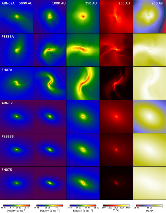
Figure 6: Mass-weighted average quantities, calculated along rays at every pixel. Rays are cast parallel to the angular momentum vector of the region in question for every column for the AMR simulations, and parallel to the Z axis for the SPH simulations. Rows correspond to simulations ABN02A, PSS83A, FH07A, ABN02S, PS83S and FH07S, and displayed values are calculated dividing mass-weighted accumulated values by the total column density at each ray. Column 1 shows density with a field of view and depth of ray integration of 5000 AU, column 2 shows density with a field of view and depth of integration of 1000 AU, and columns 3-5 show density, temperature and $\mathrm{H}_{2}$fraction with fields of view and depths of integration of 250 AU. These images were made from snapshots of the simulations at the time when their maximum density was $10^{-8}~{}\mathrm{g}~{}\mathrm{cm}^{-3}$. Color scaling is set for each column, at ($10^{-17}~{}\mathrm{g}~{}\mathrm{cm}^{-3}$, $10^{-10}~{}\mathrm{g}~{}\mathrm{cm}^{-3}$) for column 1, ($10^{-15}~{}\mathrm{g}~{}\mathrm{cm}^{-3}$, $10^{-10}~{}\mathrm{g}~{}\mathrm{cm}^{-3}$) for column 2, ($10^{-15}~{}\mathrm{g}~{}\mathrm{cm}^{-3}$, $10^{-9}~{}\mathrm{g}~{}\mathrm{cm}^{-3}$) for column 3, ($500~{}\mathrm{K}$, $3000~{}\mathrm{K}$) for column 4, and ($10^{-2}$, $0.76$) for column 5.

Figure 6 shows a comparison of the morphology of the AMR results at the final data output (when the maximum density in each simulation is $10^{-8}~{}\mathrm{g}~{}\mathrm{cm}^{-3}$) with those of the SPH simulations. The morphology of the simulations reflects the variance in the mass enclosed in the molecular cores of the different simulations, as well as the variation in their infall velocities.

Simulation ABN02A is mostly spherical, with little extended structure or gaseous filaments. The inner core of ABN02A shows no indication of angular momentum transport through a disk-like structure at this stage in the collapse. ABN02A also shows a considerably more extended, spherical high-temperature region compared to the other AMR simulations. Most interestingly, the relatively lower molecular hydrogen formation rate is evident in the smaller molecular cloud, as the fully molecular region does not even extend for $100~{}\mathrm{AU}$ from the central point of the cloud. The temperature here is strongly correlated with density and monotonically decreases with radius extending outward from the center of the cloud.

However, while ABN02A is largely spheroidal, PSS83A and FH07A both show pronounced bar-like structures. PSS83A is spheroidal at $1500~{}\mathrm{AU}$, but within $\sim 100~{}\mathrm{AU}$ there is a bar-like structure. The most dense zone of the calculation is not located at the center of the bar, and the most developed structure is at densities of $\geq 5\times 10^{-12}~{}\mathrm{g}~{}\mathrm{cm}^{-3}$. In contrast to ABN02A, the temperature structure shows more variation at a fixed density; specifically, in the upper left and lower right portions of the temperature panel, we see variations at a given density. However, while the temperature may not track the density extremely well, the molecular hydrogen fraction appears closely correlated with the density, just as we would expect given the steep $n^{3}$ density dependence of the three-body $\mathrm{H}_{2}$ formation process. Additionally, the temperature structure of the cloud encodes the shocked state of the gas, and small ripples are visible in the temperature structure, indicating both memory of the non-equilibrium molecular hydrogen formation and the kinematic state of the gas. The molecular cloud also closely tracks the bar, although we note that this is only true for molecular hydrogen fractions of $\geq 0.3$, as there is a substantial partially-molecular cloud outside the bar structure as well.

FH07A shows the most pronounced bar, with strong density contrasts between the arms and the embedding medium. The bar, like that in the PSS83A simulation, is most evident starting at densities of $\geq 5\times 10^{-12}~{}\mathrm{g}~{}\mathrm{cm}^{-3}$, which in the case of this simulation extend out to $\sim 1000~{}\mathrm{AU}$, although they are compressed along the axis of the bar. This structure is also evident in the temperature structure, but most importantly we note that it is embedded within the molecular cloud, which extends well beyond the highest density regions.

We see no evidence of advanced stages of fragmentation in any of the AMR simulations; however, the extremely compressed spiral arms of FH07A may become gravitationally unstable at later times, depending on the subsequent evolution of the angular momentum. Simulation PSS83A shows a broadly spherical mass-distribution on the scale of $2500~{}\mathrm{AU}$, but a substantially less symmetrical, nearly cardiod-shaped mass-distribution on scales of $\sim 500~{}\mathrm{AU}$.

The SPH simulations show considerably less of the fine detail apparent in the AMR simulations, due primarily to their considerably lower effective resolution on these scales. All three SPH runs show a largely spheroidal morphology, but the same basic trend is visible here as in the AMR simulations. Run ABN02S is the most spherical, while runs PSS83S and FH07S display increasingly flattened gas distributions, and the beginning of a bar is visible in the FH07S run. Run ABN02S has the highest internal temperature, as reflected in the radial profiles, as well as the most spherical shape in the inner $250~{}\mathrm{AU}$ cloud; however, we note that it is oblate at larger scales ($\sim 1000~{}\mathrm{AU}$), and that the molecular hydrogen morphology tracks the density structure. As expected from the radial profiles discussed above, and in keeping with the results from ABN02A, the ABN02S molecular hydrogen cloud is the smallest of the clouds of the three SPH simulations.

3.4 Accretion Rates

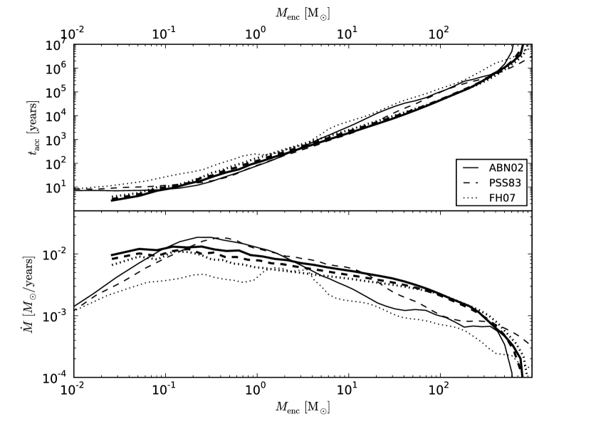
Figure 7: Radially-binned, spherically averaged accretion times (top) as a function of enclosed mass, and the accretion rates (bottom) for each mass shell. These values were calculated at the final output time of the simulation. Thin lines correspond to the AMR simulations and thick lines correspond to the SPH simulations.

In Figure 7, we plot the accretion rates and accretion times as a function of enclosed mass, calculated at the final output time of both sets of simulations.

In the top panel, we plot the accretion time. Taking $v_{r}$ as the radial velocity at the radius $r$ and $M_{\mathrm{enc}}$ as the mass enclosed within a given radius, the accretion time is given by

$$t_{\mathrm{acc}}=\frac{M_{\mathrm{enc}}}{4\pi\rho v_{r}r^{2}}.$$

For enclosed masses of less than $\sim 2~{}\mbox{M}_{\odot}$, the two sets of simulations show good agreement in the ordering of the accretion times; the FH07 runs have the longest accretion times, then the PSS83 runs, with the ABN02 runs having the shortest accretion times. However, for enclosed masses greater than $2~{}\mbox{M}_{\odot}$, the AMR simulation ABN02A increases with respect to the mean, and the ordering between the SPH and AMR simulations is no longer identical. Additionally, at the specific mass of $\sim 2~{}\mbox{M}_{\odot}$ the six simulations converge on a time scale of $\sim 300~{}\mathrm{years}$ for that mass to accrete onto the most dense zone, assuming direct infall. We note that this is approximately the mass scale of the molecular cloud in all six simulations, and thus convergence between the rates at this point is not surprising.

Considering only the accretion times between enclosed masses of $10-100~{}\mbox{M}_{\odot}$, we see variation of up to a factor of two within the AMR simulations, but relatively close convergence within the SPH calculations. This is not surprising: as discussed earlier, the AMR calculations in general show much greater variation of morphology and radial velocity as a function of the three-body rate used. However, at enclosed masses of $\sim 100~{}\mbox{M}_{\odot}$ we note that the AMR simulations show good agreement, diverging slightly at greater enclosed mass, which we can attribute to a change in the settling of the cloud as a result of time delay between the simulations.

The accretion rates, like the accretion times, show substantial variation at all mass scales. In particular, the ABN02A simulation has the highest accretion rate, peaking at $0.02~{}\mbox{M}_{\odot}~{}\mathrm{yr}^{-1}$ at $0.2~{}\mbox{M}_{\odot}$ enclosed. Simulations ABN02A and PSS83A show steeper curves in the change of accretion rate with enclosed mass than the SPH calculations, but FH07A is generally more irregular as a function of enclosed mass; we attribute this to its highly aspherical collapse, in contrast to the more spheroidal ABN02A and PSS83A calculations.

4 Discussion

Our simulations have shown that as we decrease the three-body $\mathrm{H}_{2}$ formation rate, we find several systematic changes in the properties of the collapsing gas. The molecular region at the center of the collapse becomes significantly smaller, and the density structure of this central region changes, becoming less compact and more spherical, with less small-scale structure. In addition, the time taken for the gas to collapse becomes longer. These general features appear to be independent of our choice of simulation technique or dark matter halo, although our two sets of simulations do show some disagreements on the magnitude of these differences.

These general differences are simple to relate to the microphysics of the gas. It should be no surprise that if we reduce the rate of $\mathrm{H}_{2}$ formation, then we find that the molecular fraction at a given density decreases. It is also not particularly surprising that if we reduce the amount of $\mathrm{H}_{2}$ present in gas of a given density, thereby reducing the ability of the gas to cool efficiently, then we find that the gas becomes warmer than it would be if more $\mathrm{H}_{2}$ were present (with attendant effects, e.g. Turk et al. 2010a.) What is potentially more surprising is that the large changes in $\mathrm{H}_{2}$ abundance that we see between radii of a few hundred and a few thousand AU do not have a greater effect on the temperature structure of the gas. However, this is in part a consequence of the steep dependence of the $\mathrm{H}_{2}$ cooling rate on temperature: an increase in temperature of only a few hundred Kelvin can offset a considerable reduction in the $\mathrm{H}_{2}$ abundance. In addition, chemical heating of the gas is also significantly lower in simulations with smaller three-body rates, for obvious reasons.

The consequences of the less efficient cooling and the delayed collapse of the gas are less straightforward. Naively, we might expect that if the collapse is delayed, then there will be more time for the outward transport of angular momentum, resulting in a gas distribution with less rotational support, and hence a higher infall velocity. In practice, although some of our runs support this picture (e.g. run FH07A), others suggest that this is an oversimplification. Reducing the three-body $\mathrm{H}_{2}$ formation rate, and hence delaying the collapse, leads to less rotational support at some radii, but it also leads to greater support at other radii. Moreover, the details appear to depend on the particular realization of collapse studied. Nevertheless, the general lesson that we can learn from the simulations is that the uncertainty in the three-body $\mathrm{H}_{2}$ formation rate significantly limits our ability to model the density, temperature and velocity structure of the gas close to the center of the collapse.

The consequences of this uncertainty are not easy to assess, given our lack of knowledge regarding exactly what happens following the formation of the initial Population III protostar. Many models for the later accretion phase presuppose the formation of an accretion disk around this protostar (e.g. Tan & McKee, 2004; Stacy et al., 2010; Turk et al., 2010c; Clark et al., 2010) Our simulation results clearly demonstrate that the mass assembly history of any such disk would be uncertain, given the uncertainties in the collapse time and collapse structure of these clouds. At one extreme, simulation FH07A forms an extremely strong spiral-bar structure with strong rotational support; at the other extreme, ABN02A is almost a spherically-symmetric collapse with a markedly higher accretion time.

At very early times during the formation of the central protostar and the initial assembly of the disk, we would not expect to see significant differences. The thermodynamics of the very dense gas that forms the initial protostar is controlled by the dissociation of molecular hydrogen, and is independent of our choice of three-body $\mathrm{H}_{2}$ formation rate (Yoshida et al., 2008). However, the larger-scale regions in which we see more substantial deviations in density, temperature and velocity structure, will control the rate at which gas is fed onto the disk, and thence onto the newly formed hydrostatic core. Higher accretion rates onto the disk may make it more unstable, and hence more likely to fragment (e.g. Kratter et al. 2010). Higher accretion rates onto the protostar may dramatically change the character of the radiative feedback from it, and hence may substantially alter its final mass (Omukai & Palla, 2003). Furthermore, the speed of larger-scale accretion will change the mass and radius at which the initial collapse of the gas becomes fully adiabatic. Entering the adiabatic phase of collapse at lower densities leads to a larger radii for adiabatic compression and thus a larger mass scale.

Of potentially more relevance to the final mass of Pop. III stars is the variation in the collapse times discussed in §3.1. It has been demonstrated that the gas in minihalos may contain sufficient structure to allow it to fragment during the collapse (Turk et al., 2009). If this occurs, then rather than all of the mass accreting onto one central protostar, it must now be shared amongst the multiple stars making up the protostellar system. However the ability of structure to survive will depend strongly on both the temperature of the gas and the time that it takes to collapse, since together these determine the time during which sound waves can act to remove the anisotropies. As discussed in §3.1, simulations FH07A and FH07S collapse between 20,000 and 140,000 years faster than simulations ABN02A and ABN02S. By comparison, at densities of around $10^{-16}~{}\mathrm{g}~{}\mathrm{cm}^{-3}$, the point at which the three-body reactions start to become important, the free-fall time in the gas is only $\sim 6700$ yr. We would therefore expect the details of the fragmentation to depend on the rate at which the $\mathrm{H}_{2}$ forms, as well as the details of calculations of the optically-thick cooling rate of $\mathrm{H}_{2}$.

Finally, it is also clear from our study that the differences between different numerical realizations of Population III star formation are often as large or larger than the uncertainties introduced by our lack of knowledge regarding the three-body $\mathrm{H}_{2}$ formation rate. This fact limits our ability to make general statements about the impact of the rate coefficient uncertainty on e.g. the Population III IMF. However, we can in principle address this by performing a large ensemble of simulations, so as to fully explore the entire parameter space of initial conditions (see e.g. O’Shea & Norman 2007, or Turk et al. 2010natexlabd), but we cannot eliminate the rate coefficient uncertainties in this fashion.

5 Conclusions

We have shown that the uncertainty in the rate coefficient for the three-body formation of molecular hydrogen from atomic gas has a significant effect on the details of the collapse of primordial star-forming clouds in the high-density regime. The differences in outcome brought about by choosing a different rate coefficient are most dramatic in what is typically considered the inner cloud, where the protostellar disk will begin to form, but we can reasonably expect these changes to propagate outwards over the course of the accretion onto the protostellar core.

The density scale at which molecular hydrogen forms dramatically changes the chemical makeup, morphology and velocity structure of the gas in the inner regions of the protogalactic gas cloud. In the isothermal collapse model, the accretion rate is governed by the sound speed; therefore a higher temperature, as a result of later molecular formation, results in a higher accretion rate.

The differences between runs with different three-body $\mathrm{H}_{2}$ formation rates are comparable to the differences between different realizations of primordial protostellar collapse. However, the latter issue can be addressed simply by simulating a large number of different realizations (e.g. Turk et al. (2010natexlabd)), which will allow the natural variance in collapse rates, degree of rotational support, etc. to be studied and quantified. The uncertainty in the outcome of collapse caused by our poor knowledge of the three-body $\mathrm{H}_{2}$ formation rate coefficient cannot be so easily dealt with, and represents a major limitation on our ability to accurately simulate the formation of the first stars in the Universe. Furthermore, recent suggestions that metal-free star-forming clouds could fragment into multiple protostellar cores (Turk et al., 2009; Stacy et al., 2010; Clark et al., 2010) place an increased urgency on understanding the chemistry of primordial gas. Changes in the structure of the molecular cloud, on the scales of a few thousand $\mathrm{AU}$, whether as a result of time-delay in the collapse or a change in the thermal structure, could induce or suppress fragmentation.

Finally, we would like, at this point, to be able to recommend a particular rate coefficient as the best available choice, but the truth of the matter is that there seem to be few compelling reasons to prefer one choice over another from amongst the available rates. The most conservative choice would probably be to disregard the two most extreme choices (the rates from ABN02 and FH07) and take one of the rates that produces intermediate values at low temperatures, such as the rates from PSS83 or Glover (2008). Of these intermediate rates, we prefer the latter, as it is based on a relatively recent calculation of the collisional dissociation rate of $\mathrm{H}_{2}$, rather than on an extrapolation from data that is more than forty years old. Nevertheless, even this choice is at best a stopgap until more accurate values for the rate coefficient become available.

Unfortunately, the prospects of this situation improving in the near future are dim. To the best of our knowledge, there are currently no experimental groups capable of studying this process at cosmologically relevent temperatures. Indeed, such measurements may be just beyond current experimental capabilities, given the required combination of high atomic number density and high temperature (D. W. Savin, private communication). It seems likely that this will remain an unavoidable uncertainty in studies of population III star formation for some time to come.

References

- Abel et al. (2002) Abel, T., Bryan, G. L., & Norman, M. L. 2002, Science, 295, 93
- Benz (1990) Benz, W. 1990, in Numerical Modelling of Nonlinear Stellar Pulsations Problems and Prospects, ed. J. R. Buchler, 269
- Bromm et al. (2002) Bromm, V., Coppi, P. S., & Larson, R. B. 2002, ApJ, 564, 23
- Bromm & Larson (2004) Bromm, V. & Larson, R. B. 2004, ARA&A, 42, 79
- Bryan et al. (2001) Bryan, G. L., Abel, T., & Norman, M. L. 2001, ArXiv Astrophysics e-prints
- Bryan & Norman (1997) Bryan, G. L. & Norman, M. L. 1997, ArXiv Astrophysics e-prints
- Clark et al. (2010) Clark, P.C., Glover, S.C.O., Smith, R.J., Greif, T.H., Klessen, R.S., & Bromm, V., Science, submitted
- Cohen & Westberg (1983) Cohen, N. & Westberg, K. R. 1983, Journal of Physical and Chemical Reference Data, 12, 531
- Denbigh (1981) Denbigh, K.G., “The principles of chemical equilibrium, 4th edition” 1981, (CUP: Cambridge)
- Flower & Harris (2007) Flower, D. R. & Harris, G. J. 2007, MNRAS, 377, 705
- Galli & Palla (1998) Galli, D. & Palla, F. 1998, A&A, 335, 403
- Glover (2005) Glover, S. 2005, Space Science Reviews, 117, 445
- Glover (2008) Glover, S. 2008, in American Institute of Physics Conference Series, Vol. 990, First Stars III, ed. B. W. O’Shea, A. Heger, & T. Abel, 25–29
- Glover et al. (2006) Glover, S. C., Savin, D. W., & Jappsen, A. 2006, ApJ, 640, 553
- Glover & Abel (2008) Glover, S. C. O. & Abel, T. 2008, MNRAS, 388, 1627
- Glover & Jappsen (2007) Glover, S. C. O. & Jappsen, A. 2007, ApJ, 666, 1
- Glover & Savin (2009) Glover, S. C. O. & Savin, D. W. 2009, MNRAS, 393, 911
- Kratter et al. (2010) Kratter, K. M., Matzner, C. D., Krumholz, M. R., & Klein, R. I. 2010, ApJ, 708, 1585
- Kreckel et al. (2010) Kreckel, H., Bruhns, H., Čížek, M., Glover, S. C. O., Miller, K. A., Urbain, X., & Savin, D. W. 2010, Science, 329, 69
- Martin et al. (1996) Martin, P. G., Schwarz, D. H., & Mandy, M. E. 1996, ApJ, 461, 265
- Matsuda et al. (1969) Matsuda, T., Satō, H., & Takeda, H. 1969, Progress of Theoretical Physics, 42, 219
- Omukai & Palla (2003) Omukai, K. & Palla, F. 2003, ApJ, 589, 677
- Orel (1987) Orel, A. E. 1987, J. Chem. Phys., 87, 314
- O’Shea et al. (2004) O’Shea, B. W., Bryan, G., Bordner, J., Norman, M. L., Abel, T., Harkness, R., & Kritsuk, A. 2004, ArXiv Astrophysics e-prints
- O’Shea et al. (2005) O’Shea, B. W., Nagamine, K., Springel, V., Hernquist, L., & Norman, M. L. 2005, ApJS, 160, 1
- O’Shea & Norman (2007) O’Shea, B. W. & Norman, M. L. 2007, ApJ, 654, 66
- Palla et al. (1983) Palla, F., Salpeter, E. E., & Stahler, S. W. 1983, ApJ, 271, 632
- Peebles & Dicke (1968) Peebles, P. J. E. & Dicke, R. H. 1968, ApJ, 154, 891
- Regan et al. (2007) Regan, J. A., Haehnelt, M. G., & Viel, M. 2007, MNRAS, 374, 196
- Ripamonti & Abel (2004) Ripamonti, E. & Abel, T. 2004, MNRAS, 348, 1019
- Saslaw & Zipoy (1967) Saslaw, W. C. & Zipoy, D. 1967, Nature, 216, 976
- Spergel et al. (2007) Spergel, D. N., Bean, R., Doré, O., Nolta, M. R., Bennett, C. L., Dunkley, J., Hinshaw, G., Jarosik, N., Komatsu, E., Page, L., Peiris, H. V., Verde, L., Halpern, M., Hill, R. S., Kogut, A., Limon, M., Meyer, S. S., Odegard, N., Tucker, G. S., Weiland, J. L., Wollack, E., & Wright, E. L. 2007, ApJS, 170, 377
- Spergel et al. (2003) Spergel, D. N., Verde, L., Peiris, H. V., Komatsu, E., Nolta, M. R., Bennett, C. L., Halpern, M., Hinshaw, G., Jarosik, N., Kogut, A., Limon, M., Meyer, S. S., Page, L., Tucker, G. S., Weiland, J. L., Wollack, E., & Wright, E. L. 2003, ApJS, 148, 175
- Springel (2005) Springel, V. 2005, MNRAS, 364, 1105
- Stacy et al. (2010) Stacy, A., Greif, T. H., & Bromm, V. 2010, MNRAS, 403, 45
- Susa et al. (1998) Susa, H., Uehara, H., Nishi, R., & Yamada, M. 1998, Progress of Theoretical Physics, 100, 63
- Tan & McKee (2004) Tan, J. C. & McKee, C. F. 2004, ApJ, 603, 383
- Turk et al. (2009) Turk, M. J., Abel, T., & O’Shea, B. 2009, Science, 325, 601
- Turk et al. (2010a) Turk, M. J., Norman, M. L., Abel, T., 2010a, ApJ, accepted
- Turk et al. (2010b) Turk, M. J., Smith, B. D. S., Oishi, J. S., Skory, S., Skillman, S. W., Abel, T., & Norman, M. L. 2010b, ApJS, submitted
- Turk et al. (2010c) Turk, M. J., Oishi, J. S., Abel, T., Norman, M. L., 2010c, in prep.
- Turk et al. (2010natexlabd) Turk, M. J., Abel, T., Norman, M. L., 2010d, in prep.
- Yoshida et al. (2003) Yoshida, N., Abel, T., Hernquist, L., & Sugiyama, N. 2003, ApJ, 592, 645
- Yoshida et al. (2007) Yoshida, N., Omukai, K., & Hernquist, L. 2007, ApJ, 667, L117
- Yoshida et al. (2008) —. 2008, Science, 321, 669
- Yoshida et al. (2006) Yoshida, N., Omukai, K., Hernquist, L., & Abel, T. 2006, ApJ, 652, 6