Matter-wave 2D solitons in crossed linear and nonlinear optical lattices

Abstract

It is demonstrated the existence of multidimensional matter-wave solitons in a crossed optical lattice (OL) with linear OL in the $x-$direction and nonlinear OL (NOL) in the $y-$direction, where the NOL can be generated by a periodic spatial modulation of the scattering length using an optically induced Feshbach resonance. In particular, we show that such crossed linear and nonlinear OL allows to stabilize two-dimensional (2D) solitons against decay or collapse for both attractive and repulsive interactions. The solutions for the soliton stability are investigated analytically, by using a multi-Gaussian variational approach (VA), with the Vakhitov-Kolokolov (VK) necessary criterion for stability; and numerically, by using the relaxation method and direct numerical time integrations of the Gross-Pitaevskii equation (GPE). Very good agreement of the results corresponding to both treatments is observed.

I Introduction

Bose-Einstein condensates (BEC) in optical lattices (OL) are presently attracting a great deal of interest, both experimentally and theoretically Morsh ; BK , in connection with a series of physical phenomena which arise in condensed matter physics, these including Bloch oscillations BOLin ; Pitaevskii ; SKB , generation of coherent atomic pulses (atom laser) Kasevich , dynamical localization DL1-Arimondo ; BKS-DL09 ; DL2-Arimondo , Landau-Zener tunneling LZ-Arim ; LZ-KKS05 ; LZ-Arimondo09 , superfluid Mott transitions Gren , etc. The flexibility of BEC systems with respect to changes of parameters permits, indeed, to investigate these phenomena in much an easier way than in their condensed matter physics counterparts. On the other hand, BEC systems are intrinsically nonlinear and the correspondence with usual condensed matter phenomena can be established mainly in the linear regime when the interatomic interactions are detuned to zero by means of external magnetic fields using the Feshbach resonance technique Inouye . The presence of nonlinearity, however, represents an additional resource for BEC systems which leads to interesting phenomena such as the existence of localized bound states which remain stable for infinite time due to a perfect balance between nonlinearity and dispersion. In presence of a periodic potential or a linear optical lattice (LOL), these states are known as gap-solitons (they have chemical potentials located inside the band-gaps of the underlying linear band structure), which can exist for both attractive and repulsive interactions TS ; ABDKS ; Carus , this last fact being only possible due to the presence of the periodic potential. In this context, it has been shown that gap-solitons are formed through the mechanism of modulational instability of the Bloch states, at the edges of the Brillouin zone of the underlying linear periodic system KS02 . Their existence in BECs with repulsive interactions was experimentally demonstrated in Ref. Eier . Recently, the possibility of Bloch oscillations SKB , Rabi oscillations BKS-PRA09 and dynamical localization BKS-DL09 of BEC gap solitons, in presence of constant or time dependent linear forces (induced by accelerations of the OL), have also been considered. In these cases, besides the LOL, periodic spatial variations of the nonlinearity, also known as nonlinear optical lattice (NOL), have been used in order to avoid dynamical instabilities and to make the above phenomena long lived in the nonlinear regime.

In higher dimensions, LOLs were shown to be effective in stabilizing localized states against collapse or decay, leading to the formation of stable multidimensional gap-solitons BKS02 ; BMS03 . In particular, it has been shown that a one-dimensional (1D) LOL in three-dimensional (3D) space does not allow to stabilize 3D gap-solitons. This soliton stabilization becomes only possible for attractive 3D BEC subjected to the action of a 2D LOL BMS03 ; BMS04 . The possibility to stabilize solitons by means of NOL has been investigated mainly in the 1D case, for which the mathematical properties have been studied in detail, for the ground state when considering solitons supported by 1D NOL SM ; AG ; Fibich ; Garcia , as well as by combinations of linear and nonlinear OLs abdul . In the 2D case, it was shown in AGLT07 that, for conservative systems, a NOL in one direction by itself cannot give stable localized solutions in the case of attractive interactions. This fact remains true also for 2D NOLs both for attractive and repulsive interactions.

Since NOLs can be created by means of external magnetic fields via the usual Feshbach resonance technique, or by optically induced Feshbach resonances (OFR) OFR2 , it is of interest to investigate whether crossed combined linear and nonlinear optical lattices (e.g., a LOL in one direction plus a NOL in the orthogonal direction) allow to stabilize multidimensional solitons. This analysis can be relevant in the perspective of experimental observations of multidimensional solitons. In this respect, we remark that an experimental realization of a NOL was recently achieved (on the submicron scale) for a ¹⁷⁴Yb BEC using the optical Feshbach resonance technique Yamazaki . Moreover, we recall that to date no multidimensional BEC solitons in LOLs have been observed. Besides, giving the possibility of exploring alternate methods for multidimensional soliton creation, crossed combined linear and nonlinear OLs can allow to extend to a 2D setting interesting transmission and reflection phenomena of soliton wavepackets, such as matter-wave optical limiting processes and bistability phenomena considered in the 1D case for potential applications as matter-wave limiters, BEC mirrors or cavities and atomic switches dong07 ; fatkh-pre ; He .

The aim of the present paper is to investigate the existence of 2D matter-wave solitons in crossed OLs consisting of a LOL in the $x-$direction and a NOL in the $y-$direction. In particular, we show that crossed linear and nonlinear OLs allow to stabilize 2D solitons both for attractive and repulsive interatomic interactions. This will be demonstrated by means of analytical and numerical approaches: analytically, with the variational method and a multi-Gaussian ansatz; numerically, with relaxation methods and direct numerical integrations of the Gross-Pitaevskii (GP) differential equation. Due to the lattice anisotropy, the solitons display elliptical cross sections, which in our variational approach (VA) are accounted by a multi-Gaussian ansatz with different parameters for each spatial directions. Existent VA curves and corresponding stability properties of multidimensional solitons are given for several parameter values in terms of chemical potentials and total energies as functions of the number of particles, using the Vakhitov-Kolokolov (VK) criterion for the stability. The results are then compared with direct numerical integrations of the full GP equation.

The paper is structured as follows. In section II, we introduce the model equations and discuss the physical implementation of a 2D crossed linear and nonlinear lattice by using spatial modulations of the scattering length. In Section III, we use a multi-Gaussian variational approach to derive our results, presented for chemical potentials and total energies as functions of the number of atoms, for the case of 2D solitons in 2D crossed OLs, for both attractive and repulsive interactions, where the stability is investigated by the well known VK criterion. In Section IV, the results of the VA are compared with the ones obtained by direct integrations of the GPE, using both relaxation in imaginary time and real time propagations to check the stability. Finally, in Section V, the main results of the paper are briefly summarized.

II Model equations

Multidimensional BECs in 2D crossed linear and nonlinear OLs are described in the mean field approximation by the following Gross-Pitaevskii equation (GPE):

$$i\hbar\frac{\partial\psi}{\partial t}=-\frac{\hbar^{2}}{2m}\nabla_{\cal{D}}^{2}\psi-\Lambda\cos(2k\,x)\psi-g(y)|\psi|^{2}\psi,$$ (1)

where $\psi\equiv\psi({\bf r},t)$ is normalized to the number of atoms, $\nabla^{2}_{\cal D}$ denotes the Laplacian in dimension $\cal{D}=$ 2, $m$ is the atomic mass, and $\Lambda\cos(2k\,x)$ is a LOL in the $x-$direction, with strength $\Lambda$ and lattice constant $\pi/k$. The function $g(y)$ represents a NOL in the $y-$direction, produced either by spatially varying magnetic fields near a Feshbach resonance or by optically induced Feshbach resonances OFR2 . It the following we assume $g(y)$ of the form

$$g(y)=g_{0}+g_{1}\cos(2\kappa y),$$ (2)

where $g_{0}$ denotes the mean nonlinearity related to the mean $s-$wave scattering length $a_{s0}$, and $g_{1}$ is the strength of a periodic modulation of the nonlinearity in the $y-$direction, having the period $\pi/\kappa$. Note that the quasi-2D system is confined in the $z-$direction, with the effective 2D scattering length being given in terms of the 3D scattering length and some typical scale in the confined direction Petrov2001 ; Lee2002 . In this case, the parameters $g_{0}$ and $g_{1}$ are given in units of energy multiplied by some squared distance. The spatial modulation can be produced by manipulating the scattering length with a laser field tuned near a photo association transition, e.g., close to the resonance of one of the bound $p$ levels of the excited molecules. Virtual radiative transitions of a pair of interacting atoms to this level can change the value and even reverse the sign of the scattering length. One can show that a periodic variation of the laser field intensity applied in the $y-$direction of the form $I(y)=I_{0}\cos^{2}(\kappa y)$ produces a periodic variation of the atomic scattering length, such that $a_{s}(y)=a_{s0}[1+\alpha I/(\delta+I)]$, where $a_{s0}$ is the scattering length in the absence of light, $\delta$ is the frequency detuning of the light from the resonance, and $\alpha$ is a constant factor OFR2 ; SM . For weak intensities, when $I_{0}\ll|\delta|$, we have that the real part of the scattering length can be approximated by $a_{s}=a_{s0}+a_{s1}\cos^{2}(\kappa y)$, leading to a modulated nonlinearity of essentially the same form assumed in Eq. (2).

It should be remarked, however, that the creation of a NOL in a BEC, by manipulation of the scattering length in this manner, also implies some spontaneous emission loss, which is inherent in the optical Feshbach resonance techniqueFatemi -Thal . Such dissipative effects can be strongly reduced by using laser fields with sufficiently high intensity and detuned from the resonance Bauer . It is also worth pointing out that, by using a laser field to control a magnetic FR the losses can also be essentially reduced in comparison with optically induced FR. In particular, the experiment reported in Bauer demonstrates that a laser light, near the resonance with a molecular bound-to-bound transition in ⁸⁷Rb, can be used to shift the value of the magnetic field where the FR occurs. By this way, it is possible to vary the scattering length on the optical wavelength scale, without having considerable losses (about two orders of magnitude lower then in optically induced FR experiments). We also remark that periodic variations of the scattering length, induced by the usual Feshbach resonance technique using spatially periodic external magnetic fields, would lead to similar conclusions.

In the following, we adopt dimensionless units by rescaling the space and time variables, such that the variables in Eq. (1) are redefined according to $t\rightarrow(\hbar/E_{r})\,t$, ${\mathbf{r}}\rightarrow{\mathbf{r}}/k$, with $E_{r}\equiv\hbar^{2}k^{2}/2m$ being the recoil energy and ${\mathbf{r}}\equiv\{x,y,z\}$. The wavefunction is rescaled as $\psi({\mathbf{r}},t)\rightarrow ku({\mathbf{r}},t)$, in terms of which the Eq. (1) acquires the form

$${\rm i}\frac{\partial u}{\partial t}=-\left[\frac{\partial^{2}u}{\partial x^{2}}+\frac{\partial^{2}u}{\partial y^{2}}\right]-V_{l}(x)u-\Gamma(y)|u|^{2}u,$$ (3)

where

$$V_{l}(x)=\varepsilon\cos(2x),\;\;\;\Gamma(y)=\chi+\gamma\cos(\lambda\,y),$$ (4)

denote the linear and nonlinear OL interactions, respectively. In the above, $\varepsilon=\Lambda/E_{r}$, $\chi=g_{0}k^{2}/E_{r}=8\pi a_{s0}k$, $\lambda=2\kappa/k$, and $\gamma=g_{1}k^{2}/E_{r}$, with $g_{1}$ assumed as a free parameter.

III Variational Analysis

We consider localized solutions of Eq. (3) in the crossed linear and nonlinear OLs given by Eq. (4), in the cases that the mean nonlinearity $\chi$ can be both negative (repulsive interaction) or positive (attractive interaction). In order to obtain analytical estimates for the soliton existence and stability, we use the variational approach (VA) and look for solutions of the form

$$u(x,y,t)=U(x,y)\exp(-{\rm i}\mu t),$$ (5)

where $\mu$ is the chemical potential and $U(x,y)$ is a real function for the soliton profile. Due to the anisotropy of the crossed OL, having different natures and different strengths in the two directions, we expect elliptical cross sections for the soliton profiles. This feature can be accounted in our analysis of Eq. (5) by adopting the following ansatz for $U(x,y)$:

$$U(x,y)=Ae^{-(ax^{2}+by^{2})/2},$$ (6)

where $a$ and $b$ are the parameters controlling the Gaussian widths in the two directions, with $a/b$ the aspect ratio of the solution. Using this ansatz, the stationary GPE can be written as

$$\mu U+\frac{\partial^{2}U}{\partial x^{2}}+\frac{\partial^{2}U}{\partial y^{2}}+\varepsilon\cos(2\,x)U+[\chi+\gamma\cos(\lambda\,y)]U^{3}=0,$$ (7)

from which the chemical potential and corresponding total energy are, respectively, given by

$$\mu N=\int\left\{|\nabla U|^{2}-\varepsilon\cos(2x)U^{2}-[\chi+\gamma\cos(\lambda\,y)]U^{4}\right\}dx\,dy,$$

$$E=\int\left\{|\nabla U|^{2}-\varepsilon\cos(2x)U^{2}-\frac{\chi+\gamma\cos(\lambda\,y)}{2}U^{4}\right\}dx\,dy.$$

The integrations in the above and following expressions cover the 2D phase space, from $-\infty$ to $+\infty$. From the ansatz (6) it follows that the normalized number of atoms is expressed in terms of the variational parameters $A,a,b$, as:

$$N=\int U^{2}dx\,dy=\frac{A^{2}\pi}{\sqrt{ab}}.$$ (8)

The stationary GPE in (7) can be derived from the following field Lagrangian

$$L =\displaystyle\frac{1}{2} \int\left\{|\nabla U|^{2}-[\mu+\varepsilon\cos(2x)]U^{2}\right.$$ (9)

$$\left.-\frac{1}{2}\left[\chi+\gamma\cos(\lambda\,y)\right]U^{4}\right\}dx\,dy.$$

By substituting the ansatz (6) into the above Lagrangian and performing the integrations, in terms of the variational parameters $a$, $b$ and $A$, we obtain the following effective Lagrangian:

$$L_{eff} =\displaystyle\frac{A^{2}\pi}{4\sqrt{ab}} \left\{a+b-\frac{A^{2}}{2}\left[\chi+\gamma e^{-{\lambda^{2}}/{(8b)}}\right]\right.$$ (10)

$$\left.-2\left[\mu+\varepsilon e^{-{1}/{a}}\right]\right\},$$

with the corresponding total energy given by

$$E=N\left\{\frac{a+b}{2}-\frac{A^{2}}{4}\left[\chi+\gamma e^{-{\lambda^{2}}/{(8b)}}\right]-\varepsilon e^{-{1}/{a}}\right\}.$$ (11)

Then, following from $L_{eff}$, by using the Euler-Lagrange equations for the parameters $a,b,A$, we can derive the relations for the chemical potential, total energy and number of atoms. One can easily show that these relations can be written as

$$\mu = \frac{b-3a}{2}-\varepsilon\left(1-\frac{4}{a}\right)e^{-\frac{1}{a}},$$ (12)

$$N = \frac{4\pi}{a\sqrt{ab}}\;\frac{a^{2}-2\varepsilon e^{-\frac{1}{a}}}{\chi+\gamma e^{-\frac{\lambda^{2}}{8b}}},$$ (13)

$$\frac{E}{N} = \frac{b-a}{2}-\varepsilon\left(1-\frac{2}{a}\right)e^{-\frac{1}{a}},$$ (14)

with $a,b$ solutions of the transcendental equation

$$\frac{1}{b}+\gamma\frac{\lambda^{2}}{4b^{2}}\;\frac{e^{-\frac{\lambda^{2}}{8b}}}{\chi+\gamma e^{-\frac{\lambda^{2}}{8b}}}=F(a),$$ (15)

where

$$F(a)=\frac{a}{a^{2}-2\varepsilon e^{-\frac{1}{a}}}.$$ (16)

Exact analytical solutions of Eq. (15) can be obtained in the following limiting.

i) Case $\gamma=0$. In this case only the LOL in the x-direction is present and from Eq. (15) we obtain $b=1/F(a)$. By substituting this value of $b$ in Eqs. (12) and (13), we get the following parametric equations, in the $\mu-N$ space, for the existent curves of a soliton:

$$\mu = -a-\varepsilon\left(1-\frac{3}{a}\right)e^{-\frac{1}{a}},$$ (17)

$$N = \frac{4\pi}{\chi}\sqrt{1-\varepsilon\frac{2}{a^{2}}e^{-\frac{1}{a}}}.$$ (18)

Notice from Eq. (10), that this case becomes equivalent to the case with $\lambda=0$ and $\gamma\neq 0$, by replacing $\chi$ in (18) with $\chi+\gamma$. The above equations coincide with the ones of the 1D potential case investigated in Ref. BMS04 [compare the above equations with Eqs. (8) and (9) of this paper], where it was shown that the system can support 2D localized solutions only for attractive interactions. The absence of a confining potential in the $y-$direction makes the solution to be uniform in this direction. But, interestingly enough, the solution is stable if the periodic boundary conditions are adopted in the $y-$direction (line-soliton).

ii) Case $\chi=0$. In this case both the linear and the nonlinear OL are present but the mean nonlinearity is detuned to zero. Then, the Eq. (15) reduces to $4b+\lambda^{2}=4b^{2}F(a)$ and $b$ can be expressed in terms of the parameter $a$ as

$$b=\frac{1+\sqrt{1+\lambda^{2}F(a)}}{2F(a)}.$$ (19)

iii) Case $\varepsilon=0$. In this case only the NOL in the y-direction is present and from Eq. (15) we have that $F(a)=1/a$. The solutions for $\mu$ and $N$ can be conveniently expressed in terms of the parameter $b$ as:

$$\frac{a}{b}=\left[1+\frac{\lambda^{2}}{4b}\left(1-\;\frac{\chi}{\chi+\gamma e^{-\frac{\lambda^{2}}{8b}}}\right)\right]^{-1},$$ (20)

$$\mu = \frac{b}{2}\left(1-3\frac{a}{b}\right),$$ (21)

$$N = {4\pi}{\sqrt{\frac{a}{b}}}\;\frac{1}{\chi+\gamma e^{-\frac{\lambda^{2}}{8b}}}.$$ (22)

In the absence of any confinement in the $x-$ and $y-$directions (e.g., for $\varepsilon=0$ and $\gamma=0$) the above equations reproduce the known results of the 2D nonlinear Schrödinger solitons. In particular, for attractive interactions ($\chi>0$), the soliton widths in the two directions become equal ($a=b$) and the number of atoms times the nonlinearity reduces to a constant, which coincides with the norm of 2D Townes solitons townes determining the critical threshold for collapse of a soliton in 2D as $N_{cr}=4\pi/\chi$.

In the general case the solution of Eq. (15) must be found numerically.

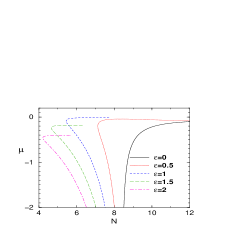
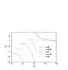
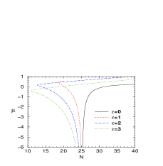
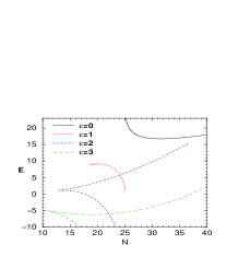
Figure 1: (Color online) Variational approach results for 2D solitons, for attractive (upper panels, with $\chi=0.5$) and repulsive (lower panels, with $\chi=-0.5$) mean nonlinearity. The chemical potentials $\mu$ are shown in the left panels, with the total energies $E$ shown in the right panels, as functions of $N$ for increasing strengths of the linear OL $\varepsilon$, as indicated inside the panels. Other parameter are fixed as $\lambda=2$, $\gamma=1.0$. All the quantities are in dimensionless units.

In Fig. 1 we show variational curves $N,\mu$ (left panels) obtained from the above equations for attractive (top) and repulsive (bottom) cases. Notice the non monotonic behavior with the appearance of a minimum (turning point) in $N$ which gives a threshold in the number of atoms for the existence of the soliton. This is a characteristic of higher dimensional solitons of cubic nonlinear Schrödinger equations. It is associated to the so called delocalizing transition BS04 ; e.g., for values of $N$ smaller than the critical value (minimum of the curve), the solution quickly decays in the uniform background and becomes fully delocalized. In the right panels of Fig. 1 we also show the corresponding plots in the $E-N$ plane. Notice that, from the general definition, $\mu=\frac{dE}{dN}$, the chemical potentials correspond to the slopes of these curves at a given $N$. Also notice that the $E-N$ curves display cusps in correspondence of the turning points of the $\mu-N$ curves.

The stability of the soliton solutions can be inferred from the observed plotted results by means of the Vakhitov-Kolokolov necessary criterion VK , according to which stable solution always correspond to the branches for which $d\mu/dN<0$. We see that no solution can be stable for both attractive and repulsive interactions in presence of only the nonlinear OL (e.g. for $\varepsilon=0$). By increasing the strength of the linear OL, however, the slope of the curves changes from positive to negative. Our analytical study therefore predicts that stable solitons in crossed linear and nonlinear OL can exist not only for attractive interactions, a fact which is true also in absence of the NOL in the $y-$direction as demonstrated in BMS04 , but also for repulsive interactions (in absence of the NOL this last case would be impossible). It is also worth to note that the stable branches of the curve in the attractive case always lie well below the critical threshold for collapse, e.g. $N<N_{cr}$.

In the next section we show that these predictions are in good agreement with the results obtained by direct numerical integrations of the GPE.

IV Numerical results and VA comparison

To check the above analytical predictions we have performed direct numerical integrations of the 2D GPE in Eq. (3) with crossed linear and nonlinear OL. The method we have used to find localized solutions is a standard relaxation algorithm in imaginary time propagation with a back-renormalization , which allows to fix the chemical potential $\mu$ and determine the corresponding number of atoms $N$ marijana .

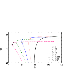
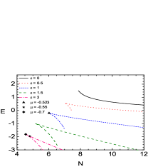
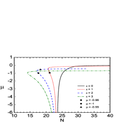
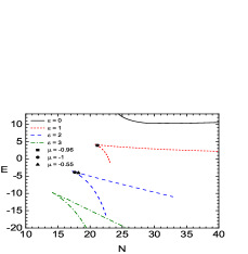
Figure 2: (Color online) Plots of 2D solitons in the $\mu-N$ (left panels) and $E-N$ (right panels) planes, as obtained from numerical integrations of Eq. (3), for attractive (upper panels, $\chi=0.5$) and repulsive (lower panels, $\chi=-0.5$) mean nonlinearity and for increasing strengths $\varepsilon$ of the linear OL (see legends inside panels). Other parameters are fixed as in Fig. 1. Symbols on curves correspond to localized solutions selected for comparison with the VA density profiles in Fig. 3 and for stability checks by time propagation in Fig. 4. All the quantities are dimensionless.

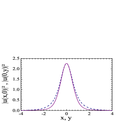
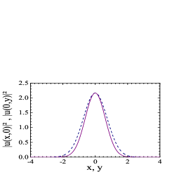
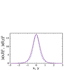
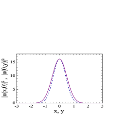
Figure 3: (Color online) Sections of the soliton density taken at $x=0$ (dashed lines) and $y=0$ (continuous lines) for attractive $\chi=0.5$ (top panels) and repulsive $\chi=-0.5$ (bottom panels) interactions. Left panels refer to the numerical GPE imaginary time relaxation method calculations and correspond to the points shown on the $\varepsilon=1.0$ curves in the upper and lower left panels of Fig. 2, at $N=6.02$ ($\mu=-0.523$) and $N=21.12$ ($\mu=-0.96$), respectively. Right panels show the soliton profiles predicted by the VA for the same chemical potentials as in the corresponding left panels. In this case, for $\mu=-0.523$, we have $N=6.2$, $a=1.3$ and $b=0.928$ (attractive case); and, for $\mu=-0.96$, we have $N=22.69$, $a=1.93$ and $b=2.6$ (repulsive case). Other parameters are fixed as in Fig. 1. All the quantities are dimensionless.

Using this method we were able to follow these solutions in the parameter space even in the regions where they become unstable (hyperbolic states), which permit us to trace curves in the $N-\mu$ plane and to determine the existence of the thresholds in the number of atoms (turning points). Typical numerical curves for 2D solitons are depicted in Fig. 2, for both attractive (top panels) and repulsive (bottom panels) interactions for different parameter values. Examples of soliton solutions determined with the relaxation method are shown in the left panels of Fig. 3. To facilitate the comparison with the VA predictions, the same set of parameters as the ones used in Fig. 1 are considered. We see that in the attractive case the agreement is very good not only qualitatively but also from a quantitative point of view. Apart from the small shift of the curves, the VA correctly predicts the existence of the turning point and the change of stability of the solutions. Notice that the agreement improves as the strength of the LOL is increased this being a consequence of the fact that in a deeper LOL the soliton becomes more localized and better described by the Gaussian ansatz used in our variational analysis. For the repulsive case the agreement becomes more qualitative with a larger shift between the numerical and the VA curves, which is unaffected by the strength of the LOL. This discrepancy can be ascribed to the fact that for repulsive interactions the Gaussian ansatz used in the VA becomes less accurate because of the tunneling of the matter into adjacent potential wells (the condensate wavefunction cannot be localized into a single potential well and develops satellites in adjacent wells of the OL).

In Fig. 3 we compare the sections of the density profiles of the solitons corresponding to the points shown on the $\varepsilon=1.0$ curves in the corresponding top and bottom left panels of Fig. 2. The right panels refer to VA solutions for attractive (top) and repulsive (bottom) cases, while the corresponding profiles obtained from numerical imaginary time integrations of the GPE are shown in the left panels. We see that, for the chosen parameters, the agreement with our analytical predictions is quite reasonable. Also notice that for the attractive case (positive mean nonlinearity) the localization induced by the LOL in the $x-$direction is stronger than the one induced by the NOL in the $y-$direction. By changing the sign of the mean nonlinearity, however, keeping all the other parameters the same, the opposite situation occurs.

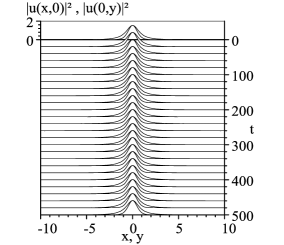
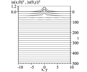
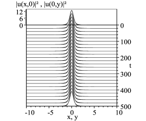
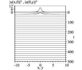
Figure 4: Time evolution of the $x$ and $y$ sections of the soliton density for attractive (top panels) and repulsive (bottom panels) interactions corresponding to the points on the stable (left panels) and unstable (right panels) branches of the $\varepsilon=2.0$ curves in the top and bottom panels of Fig. 2. The chemical potentials of the stable and unstable solitons are $\mu=-0.7$ and $\mu=-0.55$ for the attractive case, with $\mu=-1.0$ (left) and $\mu=-0.55$ for the repulsive case, respectively. In the left side of the frames we show the density scales, with the time evolution shown in the right side. Wider profiles correspond to y-sections. All the quantities are dimensionless.

The stability of these solutions has been checked by means of a real time propagation of the GPE using a Crank-Nicolson split-method and taking as initial condition slightly perturbed solitons. In the left panels of Fig. 2, we have selected four specific soliton solutions on branches of the curves, for $\varepsilon=$2, with different slope close to the turning points, to check stability, e.g. $\mu=-0.7$(diamond) and $\mu=-0.55$(star) in the attractive case(top frame); $\mu=-1.0$ (sphere) and $\mu=-0.55$(triangle) in the repulsive case (bottom frame). In Fig. 4 we show the dynamics obtained from numerical integrations of the GPE with initial conditions corresponding to these solitons with a small perturbation added. We see that while the solitons on the branch of the curves with negative slope are stable under time evolution, the ones on the branches with positive slope are unstable and quickly decay into an uniform background. These results are in agreement with what is expected from our VA analysis using the Vakhitov-Kolokolov criterion. From these studies we conclude that it is possible to create stable 2D BEC solitons using a 1D linear OL in the $x-$direction and a periodic modulation of the scattering length in the orthogonal directions, both for attractive and repulsive interactions.

An estimate of the parameters for possible experimental observations of the above 2D solitons can be made by considering, for example, the case of a repulsive BEC with $N\sim 10^{5}$ atoms of ⁸⁷Rb loaded in a crossed combined OL consisting of a LOL in the $x-$direction with a period $d=2.2\mu$m, generated by a laser field of wavelength $\pi/k\approx 0.830\mu$m and strength $\Lambda=$ 1.5 $h\times$ kHz ($h=$Planck constant), and a NOL in the $y-$direction created by an optically induced Feshbach resonance leading to a spatial variation of the scattering length of the form $a_{s}(y)=a_{s0}+a_{s1}\cos(2\kappa y)$. The background scattering length, $a_{s0}$, is obtained by using an uniform 2D external magnetic field, with the value near the FR value $B_{FR}=1007$ G, which will give $a_{s0}\approx 100a_{0}$, with $a_{0}$ denoting the Bohr radius. The modulation part of the scattering length $a_{s1}$ is induced by illuminating the system in the $y-$direction with a laser field of wavelength $\pi/\kappa\approx 0.784\mu$m, corresponding to the photo association wavelength of ⁸⁷Rb, to shift the value of $a_{s1}$ to values $Re(a_{s1}/a_{s0})\approx\pm(1-5)$Bauer . Such a crossed combined lattice is estimated to trap fundamental solitons (e.g solitons localized in a single potential well) containing up to few thousands of atoms.

V Conclusions

By summarizing our present findings, we have shown that it is possible to stabilize two-dimensional BEC solitons by combining a linear OL, in one direction, with a nonlinear OL in the other orthogonal direction, where the NOL can be obtained from a periodic modulation of the scattering length. In particular, we have shown that in 2D crossed linear and nonlinear OLs families of 2D solitons can exist and can be stable for both attractive and repulsive interactions. We have determined existent curves for chemical potentials and total energies in terms of the number of atoms, both by a Gaussian variational approach and by direct numerical integrations of the corresponding GPE. As shown, both variational and full-numerical results have been found to be in good agreement. The stability of the solutions has been checked in both cases, by using the Vakhitov-Kolokolov criterion and by direct numerical real time integrations of the GPE. In this last case, for a few set of parameters, the time evolutions of density profiles have been presented. These results open the possibility to observe two-dimensional localized matter waves in the presence of crossed linear and nonlinear optical lattices in real experiment, by using, for example, the technique considered in Ref. Bauer .

References

- (1) O. Morsh and M. Oberthaler, Rev. Mod. Phys. 78, 179 (2006).
- (2) V.A. Brazhnyi and V.V. Konotop, Mod. Phys. Lett. B 18, 627 (2004).
- (3) O. Morsch, J. H. Müller, M. Cristiani, D. Ciampini, and E. Arimondo, Phys. Rev. Lett. 87, 140402 (2001).
- (4) I. Carusotto, L. Pitaevskii, S. Stringari, G. Modugno, and M. Inguscio, Phys. Rev. Lett. 95, 093202 (2005).
- (5) M. Salerno, V.V. Konotop, Y.V. Bludov, Phys. Rev. Lett. 101, 030405 (2008).
- (6) B. P. Anderson and M. A. Kasevich, Science 282, 1686 (1998).
- (7) H. Lignier, C. Sias, D. Ciampini, Y. Singh, A. Zenesini, O. Morsch, and E. Arimondo, Phys. Rev. Lett. 99, 220403 (2007).
- (8) Yu. V. Bludov, V. V. Konotop, and M. Salerno, Europhys. Lett. 87, 20004 (2009).
- (9) A. Zenesini, H. Lignier, D. Ciampini, O. Morsch, and E. Arimondo, Phys. Rev. Lett. 102, 100403 (2009).
- (10) M. Jona-Lasinio et al., Phys. Rev. Lett. 91, 230406 (2003); S. Wimberger, R. Mannella, O. Morsch, E. Arimondo, A. Kolovsky, A. Buchleitner, Phys. Rev. A 72, 063610 (2005).
- (11) V. V. Konotop, P. G. Kevrekidis, and M. Salerno, Phys. Rev. A 72, 023611 (2005).
- (12) A. Zenesini et al., Phys. Rev. Lett. 103, 090403 (2009).
- (13) M. Greiner, O. Mandel, T. Esslinger, T.W. Hänsch and I. Bloch, Nature (London) 415, 39 (2002).
- (14) S.Inouye et al. Nature(London) 392, 151 (1998); J. Stenger et al., Phys. Rev. Lett. 82, 2422 (1999); J.L. Roberts et al., Phys. Rev. Lett. 81, 5109 (1998); S.L. Cornish, N.R. Claussen, J.L. Roberts, E.A. Cornell, and C.E. Wieman, Phys. Rev. Lett. 85, 1795 (2000); E.A. Donley et al., Nature (London) 412, 295 (2001).
- (15) A. Trombettoni and A. Smerzi, Phys. Rev. Lett. 86, 2353 (2001).
- (16) F.Kh. Abdullaev, B.B.Baizakov, S.A. Darmanyan, V.V. Konotop, and M. Salerno, Phys. Rev. A 64, 043606 (2001).
- (17) I. Carusotto, D. Embriaco, and G.C. La Rocca, Phys. Rev. A 65, 053611 (2002).
- (18) V.V. Konotop and M. Salerno, Phys. Rev. A 65, 021602 RC (2002).
- (19) B. Eiermann, Th. Anker, M. Albiez, M. Taglieber, P. Treutlein, K.-P. Marzlin, and M. K. Oberthaler, Phys. Rev. Lett. 92, 230401 (2004).
- (20) Yu. V. Bludov, V. V. Konotop, and M. Salerno, Phys. Rev. A 80, 023623 (2009).
- (21) B.B. Baizakov, V.V. Konotop, and M. Salerno, J. Phys. B 35 5105 (2002); E.A. Ostrovskaya, Yu.S. Kivshar, Phys. Rev. Lett. 90, 160407 (2003); J. Yang and Z. Musslimani, Opt. Lett. 23, 2094 (2003).
- (22) B.B. Baizakov, B.A. Malomed, and M. Salerno, Europhys. Lett. 63, 642 (2003).
- (23) B.B. Baizakov, B.A. Malomed, and M. Salerno, Phys. Rev. A 70, 053613 (2004).
- (24) H. Sakaguchi and B.A. Malomed, Phys. Rev. E 72, 046610 (2005); Phys.Rev. E 73, 026601 (2006).
- (25) F.Kh. Abdullaev and J. Garnier, Phys.Rev.A. 72, 061605 (2005).
- (26) G. Fibich, Y. Sivan, and M. I. Weinstein, Physica D 217, 31 (2006); Y. Sivan, G. Fibich, and M. I. Weinstein, Phys. Rev. Lett. 97, 193902 (2006).
- (27) J. Belmonte-Beitia, V.M. Pérez-Garcia, V. Vekslerchik, P.J. Torres, Phys. Rev. Lett. 98, 064102 (2007).
- (28) F. Abdullaev, A. Abdumalikov, and R. Galimzyanov, Phys. Lett. A 367, 149 (2007); Y. V. Kartashov, V. A. Vysloukh, and L. Torner, Opt. Lett. 33, 1747 (2008); H. Sakaguchi and B.A. Malomed, Phys. Rev. A 81, 013624 (2010).
- (29) F.Kh. Abdullaev, A. Gammal, H.L.F. da Luz, and L. Tomio, Phys.Rev.A. 76, 043611 (2007).
- (30) P.O. Fedichev, Yu. Kagan, G.V. Shlyapnikov, and J.T.M. Walraven, Phys. Rev. Lett. 77, 2913 (1996).
- (31) R. Yamazaki, S. Taie, S. Sugawa, and Y. Takahashi, Phys. Rev. Lett. 105, 050405 (2010).
- (32) G. Dong and B. Hu, Phys. Rev. A 75, 013625 (2007).
- (33) F.Kh. Abdullaev, R. M. Galimzyanov, M. Brtka, and L. Tomio, Phys. Rev. E 79, 056220(2009).
- (34) Y. He, D. Mihalacke and B. Hu, Opt.Lett. 35, 1716 (2010).
- (35) D.S. Petrov and G.V. Shlyapnikov, Phys. Rev. A 64, 012706 (2001).
- (36) M. D. Lee, S. A. Morgan, M. J. Davis, and K. Burnett, Phys. Rev. A 65, 043617 (2002).
- (37) F.K. Fatemi, K.M. Jones, and P.D. Lett, Phys.Rev.Lett. 85, 4462 (2000).
- (38) M. Theis, G. Thalhammer, K. Winkler, M. Hellwig, H. Ruff, R. Grimm, and J.H. Denschlag, Phys.Rev.Lett. 93, 123001 (2004).
- (39) G. Thalhammer, M. Theis, K. Winkler, R. Grimm, and J.H. Denschlag, Phys.Rev. A 71, 033403 (2005).
- (40) D.M. Bauer, M. Lettner, C. Vo, G. Rempe, and S. Dürr, Nature Physics 5, 339 (2009); Phys. Rev. A 79, 062713 (2009).
- (41) L. Bergé, Phys. Rep. 303, 260 (1998).
- (42) B.B. Baizakov and M. Salerno, Phys. Rev. A 69, 013602 (2004).
- (43) N.G. Vakhitov and A.A. Kolokolov, Izv. Vyssh. Uchebn. Zaved. Radiofiz. 16, 1020 (1973) [Radiophys. and Quantum Electron. 16, 783 (1973)].
- (44) M. Brtka, A. Gammal, and L. Tomio, Phys. Lett. A 359, 339 (2006).