Statistical mechanics of digital halftoning

Abstract

We consider the problem of digital halftoning from the view point of statistical mechanics. The digital halftoning is a sort of image processing, namely, representing each grayscale in terms of black and white binary dots. The digital halftoning is achieved by making use of the threshold mask, namely, for each pixel, the halftoned binary pixel is determined as black if the original grayscale pixel is greater than or equal to the mask value and is determined as white vice versa. To determine the optimal value of the mask on each pixel for a given original grayscale image, we first assume that the human-eyes might recognize the black and white binary halftoned image as the corresponding grayscale one by linear filters. The Hamiltonian is constructed as a distance between the original and the recognized images which is written in terms of the threshold mask. We are confirmed that the system described by the Hamiltonian is regarded as a kind of antiferromagnetic Ising model with quenched disorders. By searching the ground state of the Hamiltonian, we obtain the optimal threshold mask and the resultant halftoned binary dots simultaneously. From the power-spectrum analysis, we find that the resultant binary dots image is physiologically plausible from the view point of human-eyes modulation properties. We also propose a theoretical framework to investigate statistical performance of inverse digital halftoning, that is, the inverse process of halftoning. The inverse-halftoning is regarded as a special example of image restoration in which one should infer the original grayscale image from the less informative black and white binary dots. From the Bayesian inference view point, we rigorously show that the Bayes-optimal inverse-halftoning is achieved on a specific condition which is very similar to the so-called Nishimori line in the research field of spin glasses. Finally we show that both halftoning and the inverse-halftoning processes are unified under a single Hamiltonian, namely, it is possible for us to obtain the threshold mask, the halftoned and inverse-halftoned images simultaneously by finding the ground state of the spin systems.

I Introduction

Recently, a lot of problems of information science and technology have been investigated by several useful tools developed in the research field of statistical mechanics of spin glasses Mezard ; Nishi ; Bishop ; Mezard2009 . Statistical mechanics of information is now widely spreading in various subjects such as neural networks Bishop , error-correcting codes Sourlas ; Rujan ; KabashimaSaad , CDMA multi-user demodulator TanakaT , image processing, etc Bishop ; TanakaK . Especially, image restoration by making use of a graphical model of Markov random fields has been investigated extensively from both analytical and numerical point of viewsTanakaK . In the research field of image processing, digital halftoning instead of image restoration, which is defined as a process of generating a pattern of pixels with limited number of colors, especially converting a grayscale image into the binary black and white picture, has been widely used in various practical situations in media, such as the printing of newspapers, fax machines and so forth Lau ; Ulchney .

To achieve the digital halftoning, one needs the strategy to arrange the geometrical-combination of black and white pixels so as to make human-eyes to have a kind of optical illusion. Namely, the halftoning relies on the fact that the human-eyes act as a spatial low-pass filter and can not recognize any specified structure in the part of image dominated by high frequency components.

Actually, to justify this fact, several authors proposed or estimated the so-called the contrast sensitivity function, or the modulation transfer function of human visual systems independently. For instance, Analoui and Allebach Analoui introduced the contrast sensitivity function having the following form:

$$F(f_{\rho}) = k\left\{\exp(-2\pi\alpha f_{\rho})-\exp(-2\pi\beta f_{\rho})\right\}$$ (1)

where $f_{\rho}$ denotes frequency and $\alpha$ and $\beta$ are constants setting to $0.012$ and $0.046$ respectively. They set the scale parameter $k$ to satisfy the condition $\max_{f_{\rho}}F(f_{\rho})=1$, namely, $k=[(\alpha/\beta)^{-\alpha/(\alpha-\beta)}-(\alpha/\beta)^{-\beta/(\alpha-\beta)}]^{-1}\simeq 2.173938$. As another model of the human visual system, Mannos and Sakrison Mannos estimated the function as

$$F(f_{\rho}) = 2.6(0.0192+0.114f_{\rho})\exp\left[-(0.114f_{\rho})^{1.1}\right].$$ (2)

We plot the shape of these contrast sensitivity functions (1) and (2) in FIG.1.

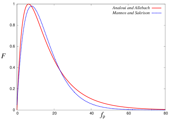
Figure 1: Human-eye modulation transfer functions estimated by Analoui and Allebach Analoui (the solid line), and Mannos and Sakrison Mannos (the broken line).

From this figure, we find that in high-frequency regime $f_{\rho}\gg 1$, the both contrast sensitivity functions decrease to zero, which means that human eyes cannot recognize high-frequency components in images. In other words, the halftone algorithm should be constructed such that the halftoned binary dots contain relatively high-frequency components to describe the original grayscale revels. This fact is an important guide for us to consider halftoning algorithms from the view point of physiology.

Up to now, to achieve fine qualities of the digital halftoning, a lot of techniques, for instance, clustered-dot ordered dither method, threshold mask method Lau ; Ulchney and blue noise mask method Mista ; Ulichney2 , error-diffusion method Floyd , etc. have been proposed and developed by many researchers. However, no attempt has been done to formulate the important problem from the view point of statistical mechanics of information. It is not difficult for us to assume that each pixel for the halftone and the grayscale images is represented by Ising spin and Q-Ising spin (or Potts spin), respectively. Therefore, it seems that statistical mechanical approach is very useful for the problem.

On the other hand, to retrieve the original grayscale image from the halftone binary dots, the so-called inverse-halftoning has been also developed especially in scanner technology Inoue2007 ; Saika2009 . As such an inverse halftoning strategy, the conventional smoothing filters have been used widely. However, it is worth while for us to look for the alternative or reconsider the problem from the view point of statistical mechanics of disordered spin systems.

In this paper, we propose a statistical-mechanical modeling of both digital halftoning and the inverse process, namely, inverse-halftoning. To attempt to generate the halftoned binary dots, we first introduce a threshold mask matrix with the same size as the original image. For the threshold mask, each pixel of the halftoned image is determined as a black pixel if the value of the original grayscale pixel is greater than the component of the threshold mask matrix and is determined as a white pixel vice versa. Then, we assume that human eyes might recognize the original grayscale image by a linear filter. By taking into account that the distance between the original and the recognized images is written in terms of the threshold mask, we naturally introduce a Hamiltonian to be minimized to determine the optimal threshold mask as the ground state. We explicitly show that the system described by the Hamiltonian is a variant of the antiferromagnetic Ising model with disorders. For a demonstration of our method to generate the optimal threshold mask, computer simulations of simulated annealing Kirkpatrick ; Geman is carried out. To investigate the statistics of the threshold mask image and the halftoned image, we evaluate the power-spectrum numerically.

On the other hand, in order to investigate statistical performance of the inverse digital halftoning, in our previous study Inoue2007 , we introduced the standard regularization theory for a Markov random-fields model to represent original grayscale image and construct the inverse process as a kind of image reconstruction of the grayscale image from a given halftone binary dots. Then, we evaluated the statistical performance by making use of Markov chain Monte Carlo (MCMC) simulations and analysis of the infinite-range mean-field model. We also investigated the inverse-halftoning process as a dynamics of disordered spin systems. In this paper, we reconsider the inverse halftoning problem from the Bayesian inference point of view. We show that the Bayes-optimal inverse-halftoning that minimizes the mean square error is achieved on a specific condition which is similar to the so-called Nishimori line Nishi1981 in the research field of spin glasses. Finally we discuss the possibility that both halftoning and the inverse-halftoning processes are unified under a single Hamiltonian, namely, we argue whether it is possible for us to obtain the threshold mask, the halftoned and inverse-halftoned images simultaneously by finding the ground state of the spin systems or not.

This paper is organized as follows. In the next Sec. II, we explain our procedure to generate the optimal threshold mask for a given original grayscale image. In this section, the Hamiltonian is introduced as a function of the threshold mask under the assumption that the human-eyes might recognize the halftoned image as the corresponding original grayscale version by a linear filter. In Sec. III, we solve the combinatorial optimization problem described by the Hamiltonian by making use of the simulated annealing. We show the resulting halftoned image for a standard grayscale image. We find that our algorithm generates the binary dots which induce the illusion of a continuous-tone image. We also investigate the power-spectrum statistics of the threshold mask array and the halftoned image. In Sec.IV, we formulate our inverse-halftoning procedure based on the MPM estimation of Bayesian statistics. We show clearly that the Bayes-optimal inverse-halftoning that minimizes the mean-square error is achieved on a specific condition. In Sec. V, we discuss the possibility that both halftoning and the inverse-halftoning processes are unified under a single Hamiltonian. The last section is summary.

II Statistical-mechanical modeling of halftoning

We first deal with the ‘forward problem’ of the digital halftoning. In this section, we first explain the procedure to generate the binary dots to represent the original grayscale image via what we call threshold dither method Lau ; Ulchney . Then, we explain how one formulates the halftoning processes as a problem of disordered spin systems and why statistical mechanics of information is useful for the problem.

II.1 Halftoning by threshold dither method

Let us first define the original grayscale image located on the square lattice with size $L_{1}\times L_{2}$ by

$$g = \left\{g_{x,y}\in 0,1,\cdots,Q-1|x=1,2,\cdots,L_{1},y=1,2,\cdots,L_{2}\right\}.$$ (3)

To generate the binary dots to represent the grayscale image $g$, we introduce the threshold mask matrix with the size $l_{1}\times l_{2}$ ($l_{1}\leq L_{1},l_{2}\leq L_{2}$):

$$t = \left\{t_{x,y}\in 0,1,\cdots,Q-1|x=1,2,\cdots,l_{1},y=1,2,\cdots,l_{2}\right\}$$ (4)

We should keep in mind that each component of the matrix $t_{x,y}$ should be satisfied the following periodic boundary condition:

$$t_{x,y}=t_{x\pm l_{1},y}=t_{x,y\pm l_{2}},\,\,\,\,L_{1}\equiv 0\,\,\,({\rm mod}\,\,l_{1}),\,\,L_{2}\equiv 0\,\,\,({\rm mod}\,\,l_{2}).$$ (5)

Then, the halftoned image is defined by

$$h = \left\{h_{x,y}\in 0,1|x=1,2,\cdots,L_{1},y=1,2,\cdots,L_{2}\right\}$$ (6)

and each pixel in the $h$ is calculated as

$$\forall_{x,y}\,\,\,\,\,\,h_{x,y} = \Theta(g_{x,y}-t_{x,y}),$$ (7)

where the step function $\Theta(x)$ is defined conventionally as

$$\Theta(x) = \left\{\begin{array}[]{cc}1&(x\geq 0)\\ 0&(x<0)\end{array}\right..$$ (10)

For this setup of the halftoning procedure, a pixel of the resulting halftoned binary image is set to one if the pixel of the original grayscale image is greater than or equal to the corresponding pixel of the threshold mask; otherwise the pixel is set to zero.

For instance, the digital halftoning is achieved by threshold mask of Bayers’ type for $Q=16$ with size $l_{1}\times l_{2}=4\times 4$:

$$\left(\begin{array}[]{cccc}t_{1,1}&t_{1,2}&t_{1,3}&t_{1,4}\\ t_{2,1}&t_{2,2}&t_{2,3}&t_{2,4}\\ t_{3,1}&t_{3,2}&t_{3,3}&t_{3,4}\\ t_{4,1}&t_{4,2}&t_{4,3}&t_{4,4}\end{array}\right) = \left(\begin{array}[]{cccc}0&8&2&10\\ 12&4&14&6\\ 3&11&1&9\\ 15&7&13&5\end{array}\right)$$ (19)

Namely, for a part with size $4\times 4$ of the original image $g$, say, for

$$\left(\begin{array}[]{cccc}g_{1,1}&g_{1,2}&g_{1,3}&g_{1,4}\\ g_{2,1}&g_{2,2}&g_{2,3}&g_{2,4}\\ g_{3,1}&g_{3,2}&g_{3,3}&g_{3,4}\\ g_{4,1}&g_{4,2}&g_{4,3}&g_{4,4}\end{array}\right) = \left(\begin{array}[]{cccc}5&5&5&5\\ 5&5&4&4\\ 4&4&4&4\\ 4&4&4&4\end{array}\right),$$ (28)

we have the corresponding block of the halftone image $h$ as

$$\left(\begin{array}[]{cccc}h_{1,1}&h_{1,2}&h_{1,3}&h_{1,4}\\ h_{2,1}&h_{2,2}&h_{2,3}&h_{2,4}\\ h_{3,1}&h_{3,2}&h_{3,3}&h_{3,4}\\ h_{4,1}&h_{4,2}&h_{4,3}&h_{4,4}\end{array}\right) = \left(\begin{array}[]{cccc}\Theta(g_{1,1}-t_{1,1})&\Theta(g_{1,2}-t_{1,2})&\Theta(g_{1,3}-t_{1,3})&\Theta(g_{1,4}-t_{1,4})\\ \Theta(g_{2,1}-t_{2,1})&\Theta(g_{2,2}-t_{2,2})&\Theta(g_{2,3}-t_{2,3})&\Theta(g_{2,4}-t_{2,4})\\ \Theta(g_{3,1}-t_{3,1})&\Theta(g_{3,2}-t_{3,2})&\Theta(g_{3,3}-t_{3,3})&\Theta(g_{3,4}-t_{3,4})\\ \Theta(g_{4,1}-t_{4,1})&\Theta(g_{4,2}-t_{4,2})&\Theta(g_{4,3}-t_{4,3})&\Theta(g_{4,4}-t_{4,4})\end{array}\right)=\left(\begin{array}[]{cccc}1&0&1&0\\ 0&1&0&0\\ 1&0&1&0\\ 0&0&0&0\end{array}\right).$$ (41)

In FIG. 2, we show a typical example of the original grayscale image ($256$ grayscale levels: left panel), the image with reduced grayscales $Q=16$: center panel) and the resulting halftone image obtained by the Bayer’s threshold mask (19). The size of the image is $L_{1}\times L_{2}=256\times 256$ and the number of the grayscale levels is $256$. Here we first converted the original $256$-grayscales $\mbox{\boldmath$g$}^{{}^{\prime}}$ image to the reduced $|\mathbb{N}(x,y)|=Q(<256)$-grayscale image $g$ by the following transform:

$$C(x:Q) = \sum_{k=0}^{Q-1}k\left\{\Theta\left(x-\frac{256}{Q}(k+1)\right)-\Theta\left(x-\frac{256}{Q}k\right)\right\}$$ (42)

and used $\forall_{x,y}\,\,\,g_{x,y}=C(g^{{}^{\prime}}_{x,y}:Q)$ as the original pixel in (7).

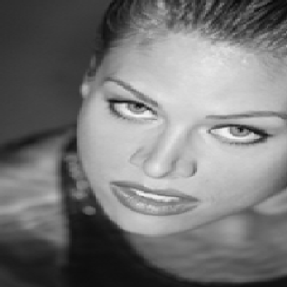
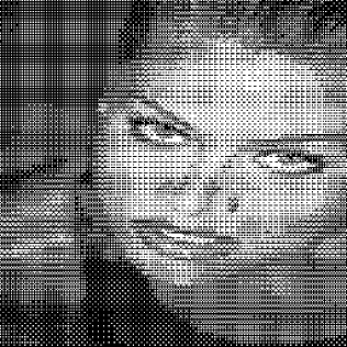
Figure 2: An example of digital halftoning by using the Bayers’ matrix (19). The $256$-grayscale image (left) and the original images in which the grayscale levels are reduced from $256$ to $16$ (center). The right panel shows the halftoned image obtained by the dither method of (19). We set $Q=16$ and $L_{1}\times L_{2}=256\times 256$.

From the right panel of this figure, we find that the grayscale-levels of the image in the middle panel is described by black and white binary dots. To see the detail of the binary dots which represent the grayscale levels in the original image, in FIG. 3, we show the result focusing on a tiny part (the ‘right eye’ of the woman) of the same image in FIG. 2.

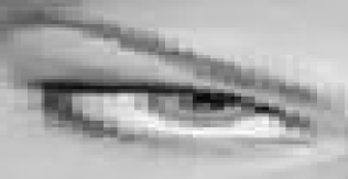
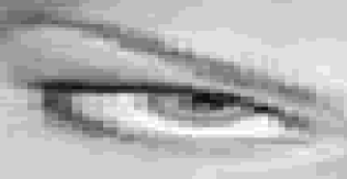
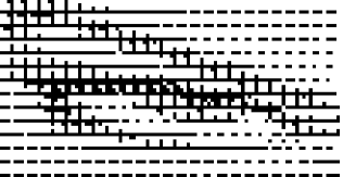
Figure 3: The result focusing on a tiny part (the ‘right eye’ of the woman) of the same image as in FIG. 2.

Therefore, once we obtain the appropriately threshold matrix $t$, the halftone binary dots $h$ is determined uniquely, and for this reason, the quality of the halftoning is dependent on how we choose the threshold mask appropriately. In this paper, we consider the case of the threshold mask having the same size as that of the original grayscale image, that is, the case of $l_{1}=L_{1},l_{2}=L_{2}$, and propose an algorithm to obtain the optimal threshold mask as lowest energy states of the Hamiltonian which is a square distance between the original and the recognized images. We shall introduce it in the next subsection.

II.2 A recognition model of human vision

As we explained in the previous subsection, our main problem is now to determine the threshold mask $t$ efficiently. For this purpose, we might assume that human eyes might retrieve the grayscale image, let us call, the recognized image:

$$s = \left\{s_{x,y}\in 0,1,\cdots,Q-1|x=1,2,\cdots,L_{1},y=1,2,\cdots,L_{2}\right\}$$ (43)

from the halftoned image $h$ by making use of the following linear filter:

$$\forall_{x,y}\,\,\,\,\,s_{x,y} = \sum_{i,j\in\mathbb{N}(x,y)}W_{x-i,y-j}\,h_{i,j},$$ (44)

where $\mathbb{N}(x,y)$ denotes the nearest neighboring pixels of the pixel located at $(x,y)$ and the point $(x,y)$ itself. Apparently, for a two-dimensional square lattice, the ingredients of $\mathbb{N}(x,y)$ are $(x,y),(x-1,y+1),(x,y+1),(x+1,y+1),(x-1,y),(x+1,y),(x-1,y-1),(x,y-1),(x+1,y-1)$ and the size is $|\mathbb{N}(x,y)|=9$. The above choice for the recognition model comes from our assumption that human-eyes might recognize a part of halftone pictures more dark when the density of black pixels located on the part is relatively high. The justification of this simple assumption could be checked by comparing the recognized image $s$, which is calculated in terms of the resultant halftone binary dots via (44), with the original grayscale image $g$. We shall discuss the results in Sec. III.

Obviously, for the simplest choice, we might set the weight $W_{x,y}$ appearing in (44) as $\forall_{x,y}\,\,\,W_{x,y}=1$. We should notice that for this choice, the spatial structure of the black dots in $\mathbb{N}(x,y)$ is not taken into account and the number $|\mathbb{N}(x,y)|$ itself determines the grayscale level of the corresponding pixel $s_{x,y}$ in the recognized image $s$. Therefore, the choice of the effective grayscale level can be controlled by choosing the number of the nearest neighboring pixels $|\mathbb{N}(x,y)|$. Taking into account this limitation, we first reduce $256$-grayscale levels to $Q(<256)$ by (42) and regard the $Q$-grayscale image as the $g$.

We also might utilize the other choice such as the following two-dimensional Gaussian-type:

$$W_{x-i,y-j} = \frac{1}{2\pi\sqrt{{\rm det}\mbox{\boldmath$\Sigma$}}}\,\exp\left[-\frac{\mbox{\boldmath$z$}^{T}\mbox{\boldmath$\Sigma$}^{-1}\mbox{\boldmath$z$}}{2}\right],\,\,\mbox{\boldmath$\Sigma$}=\left(\begin{array}[]{cc}\sigma_{x}^{2}&\rho\,\sigma_{x}\sigma_{y}\\ \rho\,\sigma_{x}\sigma_{y}&\sigma_{y}^{2}\end{array}\right),\,\,\mbox{\boldmath$z$}^{T}=(x-i,y-j).$$ (47)

For this choice, not only the number $|\mathbb{N}(x,y)|$ but also the spatial structure determines the grayscale levels in the recognized image. However, we naturally assume that the spatial structure does not affect the quality of halftoning if the size of the window $|\mathbb{N}(x,y)|$ is small enough in comparison with the image size $L^{2}$.

In this paper, we use the following specific choice of the weight $W_{x-i,x-j}$ with size $|\mathbb{N}(x,y)|=5\times 5=25$ as

$$\left(\begin{array}[]{lllll}W_{x-2,y+2}&W_{x-1,y+2}&W_{x,y+2}&W_{x+1,y+2}&W_{x+2,y+2}\\ W_{x-2,y+1}&W_{x-1,y+1}&W_{x,y+1}&W_{x+1,y+1}&W_{x+2,y+1}\\ W_{x-2,y}&W_{x-1,y}&W_{x,y}&W_{x+1,y}&W_{x+2,y}\\ W_{x-2,y-1}&W_{x-1,y-1}&W_{x,y-1}&W_{x+1,y-1}&W_{x+2,y-1}\\ W_{x-2,y-2}&W_{x-1,y-2}&W_{x,y-2}&W_{x+1,y-2}&W_{x+2,y-2}\end{array}\right) = \left(\begin{array}[]{ccccc}5&5&15&5&5\\ 5&10&15&10&5\\ 15&15&35&15&15\\ 5&10&15&10&5\\ 5&5&15&5&5\end{array}\right).$$ (58)

We should keep in mind that each recognized pixel $s_{x,y}$ takes the minimum $s_{x,y}=0$ and the maximum $s_{x,y}=255$ from the definition (44). Hence, each pixel in the recognized image $s$ calculated by (44) represents ‘defective’ $256$-grayscale levels, that is, $\forall_{x,y}\,\,\,s_{x,y}\in\{0,5,10,\cdots,255\}$.

Then, we might choose a strategy to determine the threshold mask $t$ that minimizes the square distance between the original and the recognized images. Namely, we minimize the energy $\|\mbox{\boldmath$g$}-\mbox{\boldmath$s$}\|^{2}\equiv\sum_{x=1}^{L_{1}}\sum_{y=1}^{L_{2}}(g_{x,y}-s_{x,y})^{2}$. We should notice that from the relation (44), the above distance $\|\mbox{\boldmath$g$}-\mbox{\boldmath$s$}\|^{2}$ is written in terms of the threshold mask $t$ for a given original image $g$. By substituting (44) into the distance $\|\mbox{\boldmath$g$}-\mbox{\boldmath$s$}\|^{2}$, we obtain the Hamiltonian of the system as a function of the threshold mask $t$. Thus, our digital halftoning is now reduced to a combinatorial optimization problem of the following Hamiltonian:

$$\mathcal{H}(\mbox{\boldmath$t$}|\mbox{\boldmath$g$}) = \sum_{x=1}^{L_{1}}\sum_{y=1}^{L_{2}}\left\{g_{x,y}-\sum_{i,j\in\mathbb{N}(x,y)}W_{x-i,y-j}\Theta(g_{i,j}-t_{i,j})\right\}^{2}$$ (59)

The above Hamiltonian $\mathcal{H}(\mbox{\boldmath$t$}|\mbox{\boldmath$g$})$ is a starting point of statistical-mechanical modeling of the digital halftoning. We should bear in mind that in the above Hamiltonian, $t$ are dynamical variables, whereas, $g$ are quenched disorders. As we have the Hamiltonian of the system, one can generate statistical ensembles according to standard statistical mechanics. In its thermal equilibrium at temperature $\beta^{-1}$, each possible microscopic state $t$ obeys the following Boltzmann-Gibbs distribution:

$$P_{\beta}(\mbox{\boldmath$t$}|\mbox{\boldmath$g$}) = \frac{{\exp[-\beta\mathcal{H}(\mbox{\boldmath$t$}|\mbox{\boldmath$g$})]}}{\prod_{x=1}^{L_{1}}\prod_{y=1}^{L_{2}}\sum_{t_{x,y}=0}^{Q-1}\exp[-\beta\mathcal{H}(\mbox{\boldmath$t$}|\mbox{\boldmath$g$})]}$$ (60)

One of the simplest uses of the Hamiltonian is to regard its minimum energy state as the optimal threshold mask $\hat{\mbox{\boldmath$t$}}\equiv\{\hat{t}_{x,y}\in 0,1|x=1,2,\cdots,L_{1},y=1,2,\cdots,L_{2}\}$. Namely, we have

$$\hat{\mbox{\boldmath$t$}} = \arg\max_{\mbox{\scriptsize\boldmath$t$}}P_{\beta}(\mbox{\boldmath$t$}|\mbox{\boldmath$g$}),$$ (61)

which is rewritten in terms of the statistical-mechanical terminology as

$$\forall_{x,y}\,\,\,\,\hat{t}_{x,y} = \lim_{\beta\to\infty}\prod_{x=1}^{L_{1}}\prod_{y=1}^{L_{2}}\sum_{t_{x,y}=0}^{Q-1}t_{x,y}P_{\beta}(\mbox{\boldmath$t$}|\mbox{\boldmath$g$}).$$ (62)

Calculating the $Q^{L_{1}\times L_{2}}$-sums: $\prod_{x=1}^{L_{1}}\prod_{y=1}^{L_{2}}\sum_{t_{x,y}=0}^{Q-1}(\cdots)$ and taking the zero-temperature limit are performed by Gibbs sampler with temperature annealing procedure during the Monte Carlo steps. The solution might be a good candidate for the suitable threshold mask.

We should mention that our procedure is categorized in the method ‘model-based halftoning’ which means that the threshold mask is dependent on the original image. In engineering, there exist several such algorithms Pappas ; Pappas2 ; Pappas3 . However, we should stress that these studies are completely different from our statistical-mechanical modeling.

II.3 The corresponding spin system

It is helpful for us to consider the meaning of the Hamiltonian (59) from the view point of disordered spin systems. To see the relationship between halftoning processes and the corresponding disordered spin system, we expand the square of the Hamiltonian (59). Then, we have

$$\mathcal{H}(\mbox{\boldmath$t$}|\mbox{\boldmath$g$}) = \frac{1}{2}\sum_{x=1}^{L_{1}}\sum_{y=1}^{L_{2}}\sum_{(i,j)\neq(k,l)\in\mathbb{N}(x,y)}\sum_{(k,l)\in\mathbb{N}(x,y)}J_{ij,kl}S_{i,j}S_{k,l}+\sum_{x=1}^{L_{1}}\sum_{y=1}^{L_{2}}g_{x,y}\sum_{i,j\in\mathbb{N}(x,y)}h_{i,j}S_{i,j}$$ (63)

where we defined $h_{i,j}\equiv W_{x-i,y-j}>0,J_{ij,kl}\equiv W_{x-j,y-j}W_{x-k,y-l}>0$ and $S_{i,j}={\rm sgn}(g_{ij}-t_{ij})\in\{-1,+1\}$. It should be noted that we canceled a constant term $\sum_{x=1}^{L_{1}}\sum_{y=1}^{L_{2}}(g_{x,y})^{2}$ and used the relation $\Theta(x)=(1+{\rm sgn}(x))/2$.

Thus, our system is nothing but an Ising model defined on the two-dimensional square lattice with antiferromagnetic interactions with random field $g$ on pixel. However, the ground state which minimizes the above Hamiltonian with respect to $t$ is complicated due to the quenched variables as a given original image $g$ appearing in the argument of sign function such as ${\rm sgn}(g_{ij}-t_{ij})$. The lowest energy state in the dynamical variable space of $t$ might be highly degenerated and it means that we can use various techniques developed in the field of statistical physics of disordered spin systems to obtain the lowest energy state and to investigate the lowest energy properties. In the next section, we show some demonstrations to make the halftoned binary dots that imitate the original grayscale image by minimizing the Hamiltonian (59) via simulated annealing.

III Numerical experiments

In this section, we show some demonstrations to generate the optimal threshold mask and the resulting halftoned image for a given standard grayscale image. We shall demonstrate our algorithm for one of the well-known standard images shown in FIG.4 (upper left). For the original image $g$ with the size $L_{1}\times L_{2}=400\times 400$ as input data, we construct the Hamiltonian $\mathcal{H}(\mbox{\boldmath$t$}|\mbox{\boldmath$g$})$ and carry out the calculation of the threshold mask $\hat{t}$ given by (62) via simulated annealing with the temperature schedule $\beta\sim\sqrt{t}$. For the solution of the threshold mask $\hat{t}$, we make the halftoned image $h$ according to (6).

In FIG. 4, we show the results.

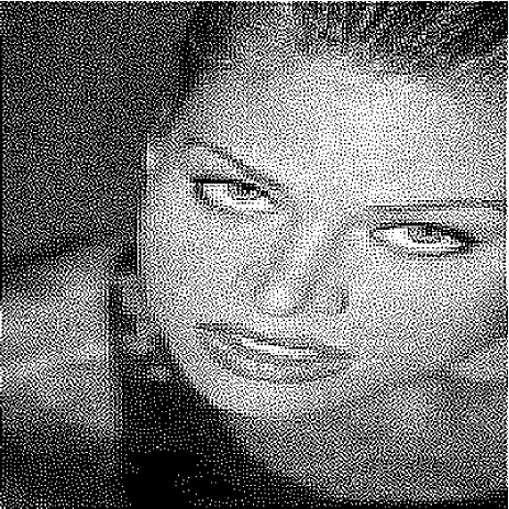
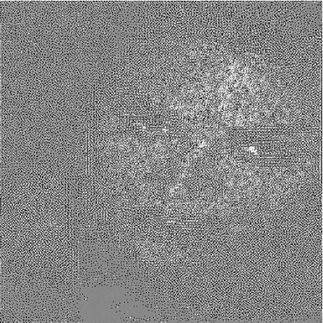
Figure 4: From the upper left to the lower right, the original image of $256$-grayscale levels, the halftoned image, the threshold mask, and the recognized image obtained by our algorithm. The size of the images is $L_{1}\times L_{2}=400\times 400$.

From the structure of the binary dots (see FIG. 4 (upper right)), we find that the resulting halftoned image looks well globally, however, locally it contains some curious clusters of vortex configurations (see FIG. 5). The similar phenomena are generally observed in the halftoned binary dots image via the error-diffusion method.

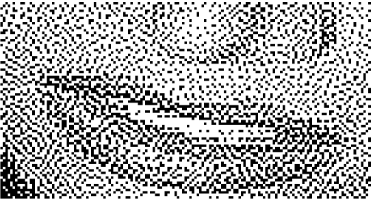
Figure 5: A part (a local structure) of the resulting halftone image (the ‘mouth’ of the woman shown in FIG. 4 (upper right)). Curious clusters of vortex configurations are observed.

In the lower right panel of FIG. 4, we show the recognized image $s$. We find that the recognized image is quite similar to the original grayscale image and this result is a justification for our assumption to construct the recognition model (44). From these pictures, we might conclude that our algorithm works very well and the resulting halftoned binary dots look fine to represent the original grayscale levels. However, it is quite important for us to evaluate the performance quantitatively. In following , we evaluate the performance of the halftoning quantitatively.

In FIG. 6 (right), we show the histograms of grayscale levels for the original and recognition images. We find that the both shapes of the histograms have a similarity, however, there is a gap between the histograms in their height. Apparently, if the perfect minimization of the Hamiltonian is achieved, these two histogram should coincide with each other. Some theoretical argument on this issue is given in Appendix A.

As we mentioned, this gap comes from the fact that the grayscale levels in the recognition image are restricted (defected) to $s_{x,y}=0,5,10,15,\cdots,255$ due to the definition of the weight $W_{x-i,y-j}$ with size $|\mathbb{N}(x,y)|\ll 256$. We discuss this issue later. In the right panel of FIG. 6, we also show the histograms of grayscale levels for the original and threshold mask. Obviously, these two histograms are completely different as we also see the difference clearly from the upper left and the lower left panels in FIG. 4.

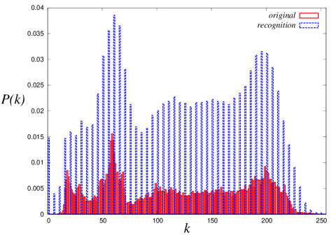
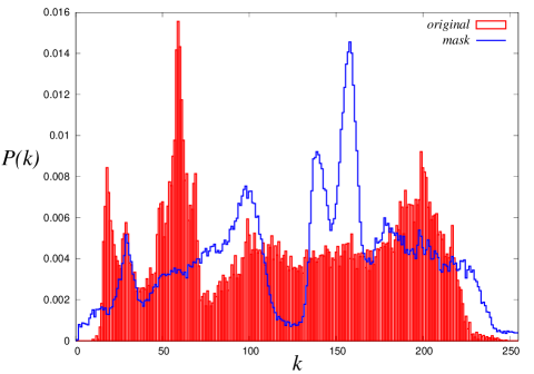
Figure 6: Histograms (empirical distributions) $P(k)$ of the grayscale levels $k\in\{0,255\}$ for the original, the mask and the recognition images.

From the view point of human visual systems, we check the power-spectrum of the threshold mask and the halftone binary dots. In order to investigate the statistical properties of the model, we next investigate the power spectrum of the threshold mask and the halftone binary dots. Namely, we evaluate

$$P_{O}(f_{x},f_{y}) = \left\{\frac{1}{L^{2}}\sum_{i,j=1}^{L}o_{i,j}\cos\left[\frac{2\pi}{L}(if_{x}+jf_{y})\right]\right\}^{2}+\left\{\frac{1}{L^{2}}\sum_{i,j=1}^{L}o_{i,j}\sin\left[\frac{2\pi}{L}(if_{x}+jf_{y})\right]\right\}^{2}$$ (64)

where we should replace $o_{i,j}$ by the threshold mask $t_{i,j}$ or the halftoned binary dots $h_{i,j}$. We should bear in mind that here we consider the case $L_{1}=L_{2}=L$.

We show the results in FIG. 7. As well-known, the so-called blue noise mask, there exists principal frequency and below the value, the power spectrum drops to zero, whereas, the high-frequency components remains finite. On the other hand, the threshold mask generated by our algorithm apparently depends on the structure of the original grayscale image.

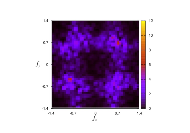
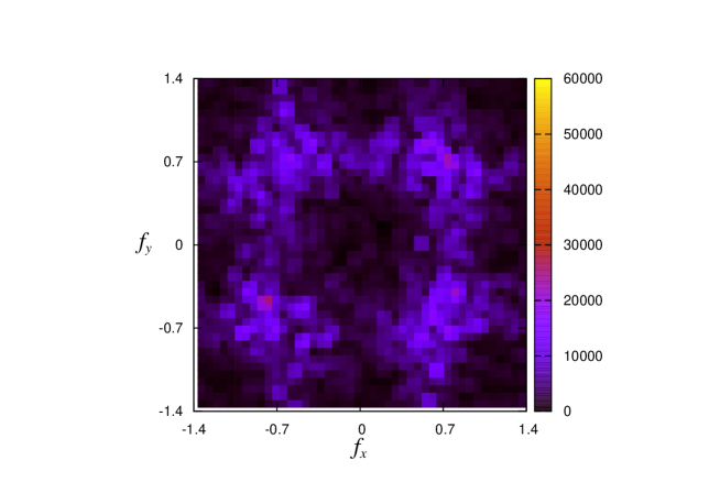
Figure 7: The power-spectrum of the halftone image (left) and threshold mask.

Therefore, it is assumed that some of the spatial structures of the original image, especially, the smoothness leading up to the low frequency components in the power spectrum remains finite. However, from the power spectrum $P_{t}(f_{x},f_{y})$ shown in FIG.8, we find that the low-frequency components almost disappear and high-frequency components remain finite.

More convenient spectrum statistics is the so-called radial-averaged power spectrum Lau defined by

$$P_{O}(f_{\rho}) = \frac{1}{N(\mathbb{R}(f_{\rho}))}\sum_{f_{x},f_{y}\in\mathbb{R}(f_{\rho})}P_{O}(f_{x},f_{y}),$$ (65)

where $\mathbb{R}(f_{\rho})$ means the region of annular rings in the Fourier space with the radiuses $f_{\rho}$ and $f_{\rho}+\Delta_{\rho}$, namely, the width of the annular rings is given by $\Delta_{\rho}$. $N(\mathbb{R}(f_{\rho}))$ is the number of frequency samples in $R(f_{\rho})$.

In FIG. 8, we plot the spectrum statistics for both threshold mask and resulting binary dots of the halftoned image.

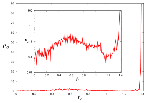
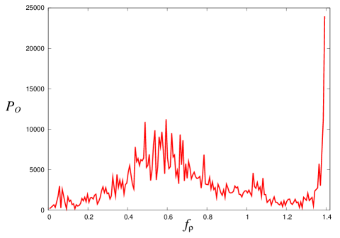
Figure 8: The radial-averaged power spectrum of the halftoned image (left) and the threshold mask (right). The inset in the left panel is the same plot as in the panel in the logarithmic scale.

Inset of FIG. 8 shows the same statistics for the threshold mask image. From this figure, we find that the low-frequency components are not dominant and relatively high-frequency components are larger than the low-frequency counter part. This tendency should be plausible from the view point of human-eyes modulation as we explained in FIG. 1.

IV Inverse digital-halftoning

In the previous sections, we consider the digital halftoning from the view point of statistical mechanics of spin systems. In engineering perspective, it is also important for us to retrieve the original grayscale image from a given halftoned binary dots when we attempt to capture the halftone image via scanner machines. The inverse problem of the digital halftoning is referred to as inverse-halftoning. In this section, we investigate the statistical performance of the inverse-halftoning by making use of the concept of statistical mechanics of disordered spin systems. Especially, we discuss the condition on which the Bayes-optimal inverse-halftoning is achieved.

IV.1 Bayesian formula

We first provide a Bayesian formula of inverse-halftoning. As we mentioned, the halftoned image $h$ is given pixel-wise as $h_{x,y}=\Theta(g_{x,y}-t_{x,y}),\forall_{x,y}$. Thus, we might regard the process as a kind of ‘channel’ which is written in terms of the following conditional probability:

$$P_{t}(\mbox{\boldmath$h$}|\mbox{\boldmath$g$}) = \frac{\prod_{x,y}\delta(h_{x,y},\Theta(g_{x,y}-t_{x,y}))}{\sum_{\mbox{\scriptsize\boldmath$h$}}\prod_{x,y}\delta(h_{x,y},\Theta(g_{x,y}-t_{x,y}))}$$ (66)

for a given threshold mask $t$. Hence, the halftoning process is regarded as stationary memory-less deterministic erasure channel from the information theoretical point of view. When we choose the ferromagnetic prior, the posterior is obtained as

$$P(\mbox{\boldmath$\sigma$}|\mbox{\boldmath$h$}:\mbox{\boldmath$t$}) = \frac{P_{t}(\mbox{\boldmath$h$}|\mbox{\boldmath$\sigma$})P_{J}(\mbox{\boldmath$\sigma$})}{\sum_{\mbox{\scriptsize\boldmath$\sigma$}}P_{t}(\mbox{\boldmath$h$}|\mbox{\boldmath$\sigma$})P_{J}(\mbox{\boldmath$\sigma$})}=\frac{{\exp}[-J\sum_{\langle(x,y)(k,l)\rangle}(\sigma_{x,y}-\sigma_{k,l})^{2}]\prod_{x,y}\delta(h_{x,y}-\Theta(g_{x,y}-t_{x,y}))}{\sum_{\mbox{\scriptsize\boldmath$\sigma$}}{\exp}[-J\sum_{\langle(x,y)(k,l)\rangle}(\sigma_{x,y}-\sigma_{k,l})^{2}]\prod_{x,y}\delta(h_{x,y}-\Theta(g_{x,y}-t_{x,y}))}$$ (67)

where we defined $\sum_{\langle(x,y),(k,l)\rangle}(\cdots)$ as a sum over the nearest neighbouring pixel pairs. From the view point of statistical mechanics, the above posterior is regarded as the Boltzmann distribution of the Q-Ising model in which the mobility of each spin is tightly constrained in the range $t_{x,y}\leq g_{x,y}\leq Q-1$ for $h_{x,y}=1$ and $0\leq g_{x,y}<t_{x,y}$ for $h_{x,y}=0$.

For the above posterior, the Maximizer of Posterior Marginal (MPM for short) estimate is given by pixel-wise optimization of the posterior as

$$\hat{\sigma}_{x,y} = \arg\max_{\sigma_{x,y}}P(\sigma_{x,y}|\mbox{\boldmath$h$}:\mbox{\boldmath$t$})$$ (68)

$$= \Theta_{Q}\left(\frac{\sum_{\mbox{\scriptsize\boldmath$\sigma$}}\sigma_{x,y}\,{\exp}[-J\sum_{\langle(x,y)(k,l)\rangle}(\sigma_{x,y}-\sigma_{k,l})^{2}]\prod_{x,y}\delta(h_{x,y}-\Theta(g_{x,y}-t_{x,y}))}{\sum_{\mbox{\scriptsize\boldmath$\sigma$}}{\exp}[-J\sum_{\langle(x,y)(k,l)\rangle}(\sigma_{x,y}-\sigma_{k,l})^{2}]\prod_{x,y}\delta(h_{x,y}-\Theta(g_{x,y}-t_{x,y}))}\right)$$

where $\Theta_{Q}(x)$ stands for a function to convert a real value $x$ to the nearest integer.

In the inverse halftoning, we should solve $\forall_{x,y}\,\,\,h_{x,y}=\Theta(g_{x,y}-t_{x,y})$ with respect to $g$ for a given halftoned image $h$ and the mask $t$.

In the reference Tadaki , one of the authors considered restoration processes of grayscale images by making use of bit-decomposed data. Namely, we generate the $Q$ binary images whose pixel is given by $\forall_{x,y}\,\,\,h_{x,y}^{(m)}=\Theta(g_{i}-m),\,m\in\{0,\cdots,Q-1\}$ and transmitting them through some noise channels. Then, the paper Tadaki dealt with the procedure to retrieve the original image $g$ from the degraded $Q$ slices of the binary images

$$\mbox{\boldmath$h^{{}^{\prime}}$}^{(m)} = \mbox{\boldmath$h$}^{(m)}+\mbox{\boldmath$\eta$}^{(m)}\,\,\,\,\,(m=0,1,\cdots,Q-1)$$ (69)

where we defined $\mbox{\boldmath$h^{{}^{\prime}}$}^{(m)}\equiv\{h^{{}^{\prime}(m)}_{x,y}|x=1,\cdots,L_{1},y=1,\cdots,L_{2}\}$ and $\mbox{\boldmath$\eta$}^{(m)}\equiv\{\eta_{x,y}^{(m)}|x=1,\cdots,L_{1},y=1,\cdots,L_{2}\}$ stands for the additive noise. If there is no degrading process, it is obvious that the vector

$$\hat{g} \equiv \sum_{m=0}^{Q-1}\mbox{\boldmath$h$}^{(m)}$$ (70)

is identical to the original grayscale image $g$. However, in the present inverse-halftoning case, the only information we have is just a single slice $\mbox{\boldmath$h$}^{(m)}$. This fact makes the problem hard to treat.

Obviously, this inverse-halftoning is a typical ill-posed problem because there are a lot of candidates to satisfy the equations. In Appendix B, we evaluate two relevant quantities, namely, degree of degeneracy for possible solutions and mutual information to evaluate the difficulties of the problem.

In the next subsection, we discuss the relationship between the so-called Bayes-optimal solution and the Nishimori line established in the research field of spin glasses.

IV.2 Bayes-optimal inverse-halftoning and the condition to achieve it

In the previous studies Saika2009 , we investigated the inverse-halftoning on the bases of Markov chain Monte Carlo simulations and analysis of the infinite-range mean-field model. Then, we found several conditions on the hyper-parameters appearing in the Hamiltonian that gives a minimum of the mean square error numerically. However, so far, we do not yet provide any mathematically rigorous results on the performance of the inverse-halftoning defined on realistic two dimensional square lattices.

In this section, we attempt to prove that the Bayes-optimal inverse-halftoning is achieved on a specific condition which is similar to the so-called Nishimori line. For the purpose, let us use here an alternative definition of pixel index. Namely, for $x,y=1,2,\cdots,L$, we change the index by means of $i=x+Ly-L,i=1,2,\cdots,L^{2}\equiv N$ (conversely, $x=(i\mod L),y=[i/L]$). Then, we consider the true prior and the true inverse-halftoning process as follows.

$$P_{J_{0}}(\mbox{\boldmath$g$}) = \frac{{\exp}[-J_{0}\sum_{ij}(g_{i}-g_{j})^{2}]}{\sum_{\mbox{\scriptsize\boldmath$g$}}{\exp}[-J_{0}\sum_{\langle ij\rangle}(g_{i}-g_{j})^{2}]},\,\,\,\,P_{t}(\mbox{\boldmath$h$}|\mbox{\boldmath$g$})=\frac{\prod_{i}\delta(h_{i},\Theta(g_{i}-t_{i}))}{\sum_{\mbox{\scriptsize\boldmath$h$}}\prod_{i}\delta(h_{i},\Theta(g_{i}-t_{i}))}$$ (71)

where we defined the original image $\mbox{\boldmath$g$}=\{g_{i}=1,\cdots,Q|i=1,\cdots,N\}$ and the halftoned image $\mbox{\boldmath$h$}=\{h_{i}=0,1|i=0,\cdots,N\}$. We also used the definition $\langle ij\rangle$ to represent all nearest neighbouring pairs on the arbitrary lattice in finite dimension. The sums $\sum_{\mbox{\scriptsize\boldmath$g$}}(\cdots)$ and $\sum_{\mbox{\scriptsize\boldmath$h$}}(\cdots)$ denote $\sum_{\mbox{\scriptsize\boldmath$g$}}=\prod_{i}\sum_{g_{i}=1,\cdots,Q}(\cdots)$ and $\sum_{\mbox{\scriptsize\boldmath$h$}}=\prod_{i}\sum_{h_{i}=0,1}(\cdots)$, respectively. It should be noted that the above likelihood is another representation of the following dither method for each pixel

$$\forall_{i}\,\,\,\,h_{i} = \Theta(g_{i}-t_{i}).$$ (72)

For this original image and the halftone process given by the likelihood (71), we naturally use the following posterior:

$$P_{J}(\mbox{\boldmath$\sigma$}|\mbox{\boldmath$h$}) = \frac{P_{t}(\mbox{\boldmath$h$}|\mbox{\boldmath$\sigma$})P_{J_{0}}(\mbox{\boldmath$\sigma$})}{\sum_{\mbox{\scriptsize\boldmath$\sigma$},\mbox{\scriptsize\boldmath$h$}}P_{t}(\mbox{\boldmath$h$}|\mbox{\boldmath$\sigma$})P_{J_{0}}(\mbox{\boldmath$\sigma$})}=\frac{{\exp}[-J\sum_{\langle ij\rangle}(\sigma_{i}-\sigma_{j})^{2}]\prod_{i}\delta(h_{i},\Theta(\sigma_{i}-t_{i}))}{\sum_{\mbox{\scriptsize\boldmath$\sigma$},\mbox{\scriptsize\boldmath$h$}}{\exp}[-J\sum_{\langle ij\rangle}(\sigma_{i}-\sigma_{j})^{2}]\prod_{i}\delta(h_{i},\Theta(\sigma_{i}-t_{i}))}$$ (73)

The quantity to be evaluated is the following mean square error $D$ for an arbitrary pixel $i$:

$$D=\mathbb{E}_{\mbox{\scriptsize\boldmath$g$},\mbox{\scriptsize\boldmath$h$}}[\{g_{i}-\Theta_{Q}(\langle\sigma_{i}\rangle_{J})\}^{2}]=\frac{\sum_{\mbox{\scriptsize\boldmath$g$},\mbox{\scriptsize\boldmath$h$}}{\exp}[-J_{0}\sum_{\langle ij\rangle}(g_{i}-g_{j})^{2}]\prod_{i}\delta(h_{i},\Theta(g_{i}-t_{i}))\left\{g_{i}-\Theta_{Q}\left(\langle\sigma_{i}\rangle_{J}\right)\right\}^{2}}{\sum_{\mbox{\scriptsize\boldmath$g$},\mbox{\scriptsize\boldmath$h$}}{\exp}[-J_{0}\sum_{\langle ij\rangle}(g_{i}-g_{j})^{2}]\prod_{i}\delta(h_{i},\Theta(g_{i}-t_{i}))}$$ (74)

where $\mathbb{E}_{\mbox{\scriptsize\boldmath$g$},\mbox{\scriptsize\boldmath$h$}}[\cdots]\equiv\int\int P_{t}(\mbox{\boldmath$h$}|\mbox{\boldmath$g$})P_{J_{0}}(\mbox{\boldmath$g$})(\cdots)d\mbox{\boldmath$g$}d\mbox{\boldmath$h$}$ and we defined the average of a single pixel over the posterior by

$$\langle\sigma_{i}\rangle_{J} \equiv \frac{\sum_{\mbox{\scriptsize\boldmath$\sigma$}}\sigma_{i}{\exp}[-J\sum_{\langle ij\rangle}(\sigma_{i}-\sigma_{j})^{2}]\prod_{i}\delta(h_{i},\Theta(\sigma_{i}-t_{i}))}{\sum_{\mbox{\scriptsize\boldmath$\sigma$},\mbox{\scriptsize\boldmath$h$}}{\exp}[-J\sum_{\langle ij\rangle}(\sigma_{i}-\sigma_{j})^{2}]\prod_{i}\delta(h_{i},\Theta(\sigma_{i}-t_{i}))}.$$ (75)

To proceed the proof, we should notice that for any stochastic variable $A$, the following fact is satisfied $\mathbb{E}_{A}[\{A-\mathbb{E}_{A}[A]\}^{2}]=\mathbb{E}_{A}[A^{2}]-\mathbb{E}_{A}[A]^{2}\,\geq\,0$, namely, $\mathbb{E}_{A}[A^{2}]\,\geq\,\mathbb{E}_{A}[A]^{2}$. When we set $A=g_{i}-\Theta_{Q}(\langle\sigma_{i}\rangle_{J})$, we have the following inequality:

$$D=\mathbb{E}_{\mbox{\scriptsize\boldmath$g$},\mbox{\scriptsize\boldmath$h$}}[\{g_{i}-\Theta_{Q}(\langle\sigma_{i}\rangle_{J})\}^{2}] \,\,\,\geq\,\,\, \left\{\mathbb{E}_{\mbox{\scriptsize\boldmath$g$},\mbox{\scriptsize\boldmath$h$}}[g_{i}]-\mathbb{E}_{\mbox{\scriptsize\boldmath$g$},\mbox{\scriptsize\boldmath$h$}}[\Theta_{Q}(\langle\sigma_{i}\rangle_{J})]\right\}^{2}$$ (76)

In following, we shall evaluate the lower bound of the $D$, that is, the right most term of the above inequality. Among the staffs of the right most part in the above inequality, $\mathbb{E}_{\mbox{\scriptsize\boldmath$g$},\mbox{\scriptsize\boldmath$h$}}[g_{i}]$ is easily evaluated as

$$\mathbb{E}_{\mbox{\scriptsize\boldmath$g$},\mbox{\scriptsize\boldmath$h$}}[g_{i}] = \frac{\sum_{\mbox{\scriptsize\boldmath$g$},\mbox{\scriptsize\boldmath$h$}}g_{i}\,{\exp}[-J_{0}\sum_{\langle ij\rangle}(g_{i}-g_{j})^{2}]\prod_{i}\delta(h_{i},\Theta(g_{i}-t_{i}))}{\sum_{\mbox{\scriptsize\boldmath$g$},\mbox{\scriptsize\boldmath$h$}}{\exp}[-J_{0}\sum_{\langle ij\rangle}(g_{i}-g_{j})^{2}]\prod_{i}\delta(h_{i},\Theta(g_{i}-t_{i}))}$$ (77)

$$= \frac{\sum_{\mbox{\scriptsize\boldmath$g$}}g_{i}\,{\exp}[-J_{0}\sum_{\langle ij\rangle}(g_{i}-g_{j})^{2}]\sum_{\mbox{\scriptsize\boldmath$h$}}\prod_{i}\delta(h_{i},\Theta(g_{i}-t_{i}))}{\sum_{\mbox{\scriptsize\boldmath$g$}}{\exp}[-J_{0}\sum_{\langle ij\rangle}(g_{i}-g_{j})^{2}]\sum_{\mbox{\scriptsize\boldmath$h$}}\prod_{i}\delta(h_{i},\Theta(g_{i}-t_{i}))}$$

$$= \frac{\sum_{\mbox{\scriptsize\boldmath$g$}}g_{i}\,{\exp}[-J_{0}\sum_{\langle ij\rangle}(g_{i}-g_{j})^{2}]}{\sum_{\mbox{\scriptsize\boldmath$g$}}{\exp}[-J_{0}\sum_{\langle ij\rangle}(g_{i}-g_{j})^{2}]}=\left(\frac{Z_{J_{0}}^{(g>t)}}{Z_{J_{0}}}\right)\,m_{i}^{(J_{0},g>t)}+\left(\frac{Z_{J_{0}}^{(g<t)}}{Z_{J_{0}}}\right)\,m_{i}^{(J_{0},g<t)}\equiv m_{i}^{(J_{0})}$$

where we defined

$$m_{i}^{(J_{0},g>t)} = \frac{\sum_{\mbox{\scriptsize\boldmath$g$}\in\{g_{i}|g_{i}>t_{i}\}}g_{i}\,{\exp}[-J_{0}\sum_{\langle ij\rangle}(g_{i}-g_{j})^{2}]}{\sum_{\mbox{\scriptsize\boldmath$g$}\in\{g_{i}|g_{i}>t_{i}\}}{\exp}[-J_{0}\sum_{\langle ij\rangle}(g_{i}-g_{j})^{2}]}$$ (78)

$$m_{i}^{(J_{0},g<t)} = \frac{\sum_{\mbox{\scriptsize\boldmath$g$}\in\{g_{i}|g_{i}<t_{i}\}}g_{i}\,{\exp}[-J_{0}\sum_{\langle ij\rangle}(g_{i}-g_{j})^{2}]}{\sum_{\mbox{\scriptsize\boldmath$g$}\in\{g_{i}|g_{i}<t_{i}\}}{\exp}[-J_{0}\sum_{\langle ij\rangle}(g_{i}-g_{j})^{2}]}$$ (79)

and

$$Z_{J_{0}}^{(g>t)} = \sum_{\mbox{\scriptsize\boldmath$g$}\in\{g_{i}|g_{i}>t_{i}\}}{\exp}[-J_{0}\sum_{\langle ij\rangle}(g_{i}-g_{j})^{2}]$$ (80)

$$Z_{J_{0}}^{(g<t)} = \sum_{\mbox{\scriptsize\boldmath$g$}\in\{g_{i}|g_{i}<t_{i}\}}{\exp}[-J_{0}\sum_{\langle ij\rangle}(g_{i}-g_{j})^{2}]$$ (81)

$$Z_{J_{0}} = \sum_{\mbox{\scriptsize\boldmath$g$}}{\exp}[-J_{0}\sum_{\langle ij\rangle}(g_{i}-g_{j})^{2}]$$ (82)

Therefore, $\mathbb{E}_{\mbox{\scriptsize\boldmath$g$},\mbox{\scriptsize\boldmath$h$}}[g_{i}]$ is identical to the local magnetization $m_{i}^{(J_{0})}$ of the pure ferromagnetic Q-Ising model having the interaction strength $J_{0}$.

On the other hand, the lest of the term appearing in the right hand side of the equation (76) is written by

$$\mathbb{E}_{\mbox{\scriptsize\boldmath$g$},\mbox{\scriptsize\boldmath$h$}}[\Theta_{Q}(\langle\sigma_{i}\rangle_{J})]$$ (83)

$$= \frac{\sum_{\mbox{\scriptsize\boldmath$g$},\mbox{\scriptsize\boldmath$h$}}{\exp}[-J_{0}\sum_{\langle ij\rangle}(g_{i}-g_{j})^{2}]\prod_{i}\delta(h_{i},\Theta(g_{i}-t_{i}))\Theta_{Q}\left(\frac{\mbox{$\sum$}_{\mbox{\scriptsize\boldmath$\sigma$}}\sigma_{i}{\exp}[-J\mbox{$\sum$}_{\langle ij\rangle}(\sigma_{i}-\sigma_{j})^{2}]\mbox{$\prod$}_{i}\delta(h_{i},\Theta(\sigma_{i}-t_{i}))}{\mbox{$\sum$}_{\mbox{\scriptsize\boldmath$\sigma$}}{\exp}[-J\mbox{$\sum$}_{\langle ij\rangle}(\sigma_{i}-\sigma_{j})^{2}]\mbox{$\prod$}_{i}\delta(h_{i},\Theta(\sigma_{i}-t_{i}))}\right)}{\mbox{$\sum$}_{\mbox{\scriptsize\boldmath$g$},\mbox{\scriptsize\boldmath$h$}}{\exp}[-J_{0}\mbox{$\sum$}_{\langle ij\rangle}(g_{i}-g_{j})^{2}]\prod_{i}\delta(h_{i},\Theta(g_{i}-t_{i}))}$$

$$= \frac{\sum_{\mbox{\scriptsize\boldmath$g$}}{\exp}[-J_{0}\sum_{\langle ij\rangle}(g_{i}-g_{j})^{2}]\Theta_{Q}\left(\frac{\mbox{$\sum$}_{\mbox{\scriptsize\boldmath$\sigma$}}\sigma_{i}{\exp}[-J\mbox{$\sum$}_{\langle ij\rangle}(\sigma_{i}-\sigma_{j})^{2}]\mbox{$\prod$}_{i}\delta(\Theta(g_{i}-t_{i}),\Theta(\sigma_{i}-t_{i}))}{\mbox{$\sum$}_{\mbox{\scriptsize\boldmath$\sigma$}}{\exp}[-J\mbox{$\sum$}_{\langle ij\rangle}(\sigma_{i}-\sigma_{j})^{2}]\mbox{$\prod$}_{i}\delta(\Theta(g_{i}-t_{i}),\Theta(\sigma_{i}-t_{i}))}\right)}{\sum_{\mbox{\scriptsize\boldmath$g$}}{\exp}[-J_{0}\sum_{\langle ij\rangle}(g_{i}-g_{j})^{2}]}$$

$$= \left(\frac{Z_{J_{0}}^{(g>t)}}{Z_{J_{0}}}\right)\Theta_{Q}\left(\frac{\mbox{$\sum$}_{\mbox{\scriptsize\boldmath$\sigma$}\in\{\sigma_{i}|\sigma_{i}>t_{i}\}}\sigma_{i}{\exp}[-J\mbox{$\sum$}_{\langle ij\rangle}(\sigma_{i}-\sigma_{j})^{2}]}{\mbox{$\sum$}_{\mbox{\scriptsize\boldmath$\sigma$}\{\sigma_{i}|\sigma_{i}>t_{i}\}}{\exp}[-J\mbox{$\sum$}_{\langle ij\rangle}(\sigma_{i}-\sigma_{j})^{2}]}\right)$$

$$+ \left(\frac{Z_{J_{0}}^{(g<t)}}{Z_{J_{0}}}\right)\Theta_{Q}\left(\frac{\mbox{$\sum$}_{\mbox{\scriptsize\boldmath$\sigma$}\in\{\sigma_{i}|\sigma_{i}<t_{i}\}}\sigma_{i}{\exp}[-J\mbox{$\sum$}_{\langle ij\rangle}(\sigma_{i}-\sigma_{j})^{2}]}{\mbox{$\sum$}_{\mbox{\scriptsize\boldmath$\sigma$}\{\sigma_{i}|\sigma_{i}<t_{i}\}}{\exp}[-J\mbox{$\sum$}_{\langle ij\rangle}(\sigma_{i}-\sigma_{j})^{2}]}\right)$$

$$= \left(\frac{Z_{J_{0}}^{(g>t)}}{Z_{J_{0}}}\right)\Theta_{Q}(m_{i}^{(J,\sigma>t)})+\left(\frac{Z_{J_{0}}^{(g<t)}}{Z_{J_{0}}}\right)\Theta_{Q}(m_{i}^{(J,\sigma<t)})$$

Therefore, the lower bound of the mean square error is evaluated as follows.

$$D \geq \{\mathbb{E}_{\mbox{\scriptsize\boldmath$g$},\mbox{\scriptsize\boldmath$h$}}[g_{i}]-\mathbb{E}_{\mbox{\scriptsize\boldmath$g$},\mbox{\scriptsize\boldmath$h$}}[\Theta_{Q}(\langle\sigma_{i}\rangle_{J})]\}^{2}$$ (84)

$$= \left\{\left(\frac{Z_{J_{0}}^{(g>t)}}{Z_{J_{0}}}\right)\left(m_{i}^{J_{0},g>t}-\Theta_{Q}(m_{i}^{J,\sigma>t})\right)+\left(\frac{Z_{J_{0}}^{(g<t)}}{Z_{J_{0}}}\right)\left(m_{i}^{J_{0},g<t}-\Theta_{Q}(m_{i}^{J,\sigma<t})\right)\right\}^{2}$$

$$= \left\{\left(\frac{Z_{J_{0}}^{(g>t)}}{Z_{J_{0}}}\right)\left|m_{i}^{J_{0},g>t}-\Theta_{Q}(m_{i}^{J,\sigma>t})\right|+\left(\frac{Z_{J_{0}}^{(g<t)}}{Z_{J_{0}}}\right)\left|m_{i}^{J_{0},g<t}-\Theta_{Q}(m_{i}^{J,\sigma<t})\right|\right\}^{2}$$

$$\geq \left\{\left(\frac{Z_{J_{0}}^{(g>t)}}{Z_{J_{0}}}\right)\delta_{1}+\left(\frac{Z_{J_{0}}^{(g<t)}}{Z_{J_{0}}}\right)\delta_{2}\right\}^{2}$$

where the equality on the last line is satisfied for $J=J_{0}$. We also used the fact that the sign of $(m_{i}^{J_{0},g>t}-\Theta_{Q}(m_{i}^{J,\sigma<t}))$ and $(m_{i}^{J_{0},g>t}-\Theta_{Q}(m_{i}^{J,\sigma<t}))$ are the same because the local magnetizations $m_{i}^{J,\sigma>t}$ and $m_{i}^{J,\sigma<t}$ are monotonically increasing function with respect to $J$. $\delta=\delta_{1},\delta_{2}$ is a quantization error due to the Q-generalized step function $\Theta_{Q}(\cdots)$ defined as

$$\Theta_{Q}(x) = x-\delta$$ (85)

From the argument we presented above, we found that the performance of the inverse-halftoning achieved by the posterior (75) is optimized on the specific condition $J=J_{0}$ which is similar to the Nishimori line (point) Nishi1981 in the research field of spin glasses.

V Simultaneous generation of mask, halftone and recognition images

Finally we show that both halftoning and the inverse-halftoning processes are unified under a single Hamiltonian, namely, it is possible for us to obtain the threshold mask, the halftoned and inverse-halftoned images simultaneously by finding the ground state of the spin systems.

In this paper, we proposed the digital halftoning and the inverse-halftoning separately. However, from the form of the Hamiltonian $\mathcal{H}(\mbox{\boldmath$t$}|\mbox{\boldmath$g$})$, the definition of the halftoned image: $\forall_{x,y}\,\,\,h_{x,y}=\Theta(g_{x,y}-t_{x,y})$ and the recognition image: $\forall_{x,y}\,\,\,s_{x,y}=\sum_{i,j\in\mathbb{N}(x,y)}W_{x-i,y-j}\Theta(g_{x,y}-t_{x,y})$, it is confirmed that these three important images are obtained simultaneously in the single theoretical framework, that is, minimizing the Hamiltonian $\cal{H}(\mbox{\boldmath$t$}|\mbox{\boldmath$g$})$ with respect to the mask $t$ for a given original image $g$.

Then, we should remember that there is a gap between the histograms of the grayscale levels for the recognition and the original images. This gap might make us hard to accept the recognition image as the inverse-halftoned one as a solution.

As we mentioned before, this gap comes from the fact that the grayscale levels in the recognition image are restricted (defected) to $s_{x,y}=0,5,10,15,\cdots,255$ due to the definition of the weight $W_{x-i,y-j}$ with size $|\mathbb{N}(x,y)|=5\times 5=25\ll 256=Q$. To reduce the gap, we might use the following linear filter:

$$\forall_{x,y}\,\,\,\,\,s_{x,y}^{(t)} = \frac{1}{|\mathbb{N}^{{}^{\prime}}(x,y)|}\sum_{k,l\in\mathbb{N}^{{}^{\prime}}(x,y)}s_{k,l}^{(t-1)},\,\,\,t=1,\cdots,n$$ (86)

where the initial condition $\mbox{\boldmath$s$}^{(0)}$ are chosen as $\forall_{x,y}\,\,\,s_{x,y}=\sum_{i,j\in\mathbb{N}(x,y)}W_{x-i,y-j}\Theta(g_{x,y}-t_{x,y})$ for the minimum energy state of the Hamiltonian $\mathcal{H}(\mbox{\boldmath$t$}|\mbox{\boldmath$g$})$. Thus, for a given $\mbox{\boldmath$s$}^{(0)}$, we recursively operate the above map (86) $n$ times, and then, one might obtain more plausible image than the $\forall_{x,y}\,\,\,s_{x,y}^{(0)}$ as the inverse-halftoned image.

We show the resulting histogram of the grayscale levels in FIG. 9 and the corrected recognition images in FIG. 10 for $n=1$ and $2$. We set the number of nearest neighbouring pixels around the pixel at $(x,y)$ as $|\mathbb{N}^{{}^{\prime}}(x,y)|=3\times 3=9$, namely, $\mathbb{N}^{{}^{\prime}}(x,y)=\{(x-1,y+1),(x,y+1),(x+1,y+1),(x-1,y),(x,y),(x+1,y),(x-1,y-1),(x,y-1),(x+1,y-1)\}$.

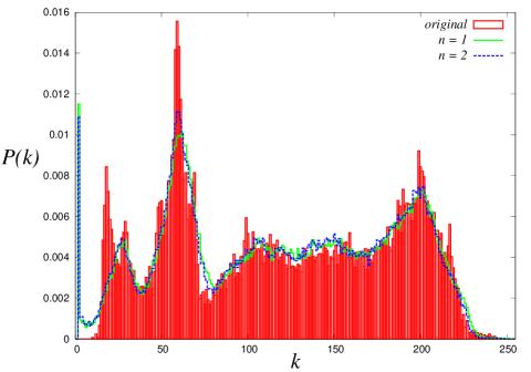
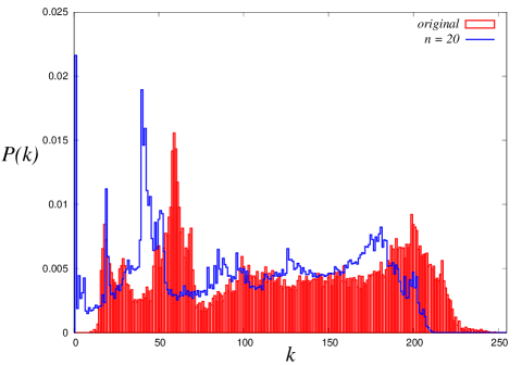
Figure 9: Histogram of grayscale levels for the original image and the recognition images after operating the linear filter (86) with $n=1,2$ (left) and $n=20$ (right).

From these figures, we find that the gap between two images actually reduced and the resulting recognition image is improved by ‘mixing effect’ on the defected grayscale levels $s_{x,y}=0,5,10,15,\cdots,255$. However, when we increase the number of iteration $n$, the mixing effect works too much on the recognition image and it makes the local structure of the image too smooth (see FIG. 9 (right) and FIG. 10 (lower right)).

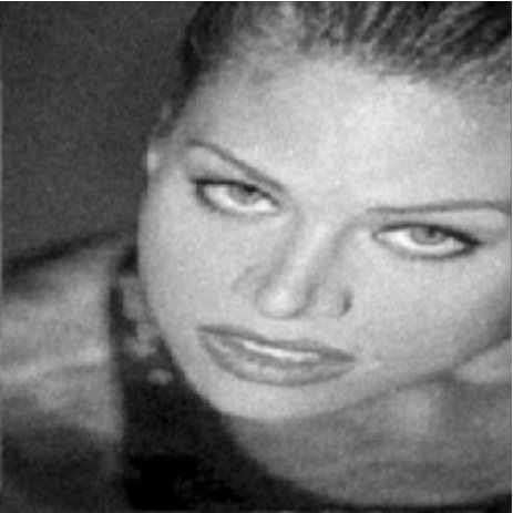
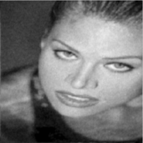
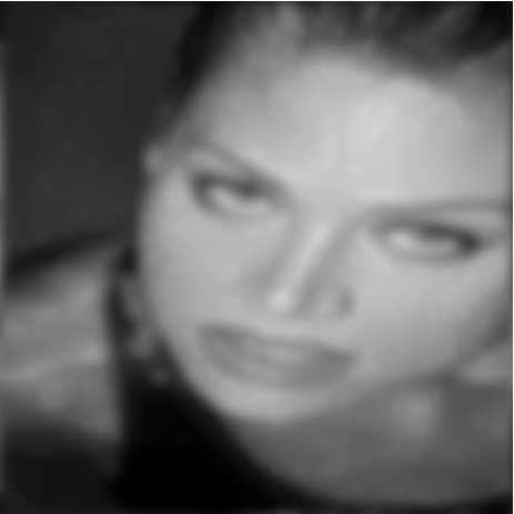
Figure 10: From the upper left to the lower right, the original image, the recognized images after operating the linear filter (86) with $n=1,2$ and $n=20$ are shown.

VI Summary

In this paper, we proposed a possible statistical-mechanical modeling for digital halftoning. This formalism helps us to understand the problem as a combinatorial optimization which is described by a sort of disordered spin systems. Finding the ground state was achieved by simulated annealing and we found that the resulting binary dots looks well to represent the original grayscale levels. The quality of the binary dots was evaluated from the power-spectrum statistics. We found that the binary dots contain relatively high frequency components which are plausible from the view point of human-eyes modulation properties. We also proposed a theoretical framework to evaluate the statistical performance of the inverse digital-halftoning based on statistical mechanics. From the Bayesian inference view point, we rigorously show that the Bayes-optimal inverse-halftoning is achieved on a specific condition which is very similar to the so-called Nishimori line in the research field of spin glasses. We hope our formulation might be applied to generating of binary halftoned images effectively and evaluating the performance for the inverse-halftoning from halftoned binary images obtained by various algorithms.

This work was financially supported by Grant-in-Aid, Scientific Research on Priority Areas Deepening and Expansion of Statistical Mechanical Informatics (DEX-SMI) of the Ministry of Education, Culture, Sports, Science and Technology (MEXT) No. 18079001. One of the authors (JI) was financially supported by Grant-in-Aid for Scientific Research (C) of Japan Society for the Promotion of Science, No. 22500195 and INSA (Indian National Science Academy) - JSPS (Japan Society of Promotion of Science) Bilateral Exchange Programme.

Appendix A Distribution of the recognized pixels

In Sec. III, we evaluated the performance of halftoning through two different measurements, namely, the histograms of grayscale levels and the power-spectrum via computer simulations. However, it might be helpful for us to evaluate the performance analytically. In this Appendix, we derive the distribution of the recognized pixels, that is, the number of black pixels in a window with $|\mathbb{N}(x,y)|=Q(\ll 256)$ analytically. Namely, we consider the distribution of the following quantities:

$$\mu_{i} = \frac{1}{Q}\sum_{l\in\mathbb{N}(i)}\Theta(g_{l}-t_{l})=s_{i}$$ (87)

where we consider the case of $L_{1}=L_{2}=L$ and defined the index $i$ so as to satisfy $i=x+Ly-L$, namely, $i$ takes $i=1,2,\cdots,L^{2}$ and we set $L^{2}=N$. It is obvious that $(x,y)$ for a given $i$ are given as $x=(i\mod L),y=[i/L]$. Here we consider the case of $|\mathbb{N}(i)|=Q=\mathcal{O}(1)$. Then, we obtain the general formula for the distribution as follows.

$$P_{\beta,Q}(\mu_{i}:\mbox{\boldmath$g$})=\frac{\prod_{i}\sum_{t_{i}=0}^{Q-1}\delta(Q\mu_{i}-\sum_{l\in\mathbb{N}(i)}\Theta(g_{l}-t_{l}))\int_{-\infty}^{\infty}\prod_{j\neq i}d\mu_{j}{\delta(Q\mu_{j}-\sum_{l\in\mathbb{N}(i)}}\Theta(g_{l}-t_{l})){\rm e}^{-\beta H_{\rm eff}}}{\prod_{i}\sum_{t_{i}=0}^{Q-1}\int_{-\infty}^{\infty}\prod_{i}d\mu_{i}{\delta(Q\mu_{i}-\sum_{l\in\mathbb{N}(i)}}\Theta(g_{l}-t_{l})){\rm e}^{-\beta H_{\rm eff}}}$$ (88)

where $\mathcal{H}_{\rm eff}$ denotes the following effective Hamiltonian:

$$\mathcal{H}_{\rm eff} = -\sum_{i}g_{i}\sum_{l\in\mathbb{N}(i)}\Theta(g_{l}-t_{l})+\sum_{i}\sum_{k,l\in\mathbb{N}(i)}\Theta(g_{l}-t_{l})\Theta(g_{k}-t_{k})$$ (89)

In the above expression, we omitted the term $\sum_{i}g_{i}^{2}$ which is independent of the dynamical variable $t$. We should keep in mind that the normalization $\int_{-\infty}^{\infty}d\mu_{i}P(\mu_{i}:\mbox{\boldmath$g$})=1$ is satisfied. It also should be noted that the pixels are fully connected in the window with size $|\mathbb{N}(i)|=Q$. Then, the effective Hamiltonian is reduced to the decoupled form $\mathcal{H}_{\rm eff}=\sum_{i}\mathcal{H}_{\rm eff}^{(i)}$ and we immediately obtain

$$\prod_{j}\sum_{t_{j}\neq t_{i}}\int_{-\infty}^{\infty}\prod_{j\neq i}d\mu_{j}\delta\left(Q\mu_{j}-\sum_{l\in\mathbb{N}(j)}\Theta(g_{l}-t_{l})\right)\,{\exp}\left(-\sum_{j\neq i}\beta H_{\rm eff}^{(j)}\right) = {\rm e}^{-(N-1)f}$$ (90)

$$\prod_{i}\sum_{t_{i}}\int_{-\infty}^{\infty}\prod_{i}d\mu_{i}\delta\left(Q\mu_{i}-\sum_{l\in\mathbb{N}(i)}\Theta(g_{l}-t_{l})\right)\,{\exp}\left(-\beta\sum_{i}H_{\rm eff}^{(i)}\right) = {\rm e}^{-Nf}$$ (91)

by using the saddle point method in the limit of $N\to\infty$. $f$ is given by $f=-\Phi(\beta,Q:\mbox{\boldmath$g$})$ with

$$\Phi(\beta,Q:\mbox{\boldmath$g$})=\log\left\{\int_{0}^{1}d\mu\int_{-i\infty}^{+i\infty}\frac{id\hat{\mu}}{\sqrt{2\pi}}{\exp}\left[-Q\hat{\mu}\mu-\frac{\beta}{2}Q^{2}\mu^{2}+\beta Qg\mu+Q\log\sum_{t=0}^{Q-1}{\rm e}^{\hat{\mu}\Theta(g-t)}\right]\right\}.$$ (92)

Then, equation (88) leads to

$$P_{\beta,Q}(\mu:\mbox{\boldmath$g$}) = \frac{{\rm e}^{-\frac{\beta}{2}Q^{2}\mu^{2}+\beta Qg\mu}\int_{-i\infty}^{+i\infty}\frac{d\hat{\mu}}{\sqrt{2\pi}}{\exp}\left[-Q\hat{\mu}\mu+Q\log\sum_{t=0}^{Q-1}{\rm e}^{\hat{\mu}\Theta(g-t)}\right]}{\int_{0}^{1}d\mu\int_{-i\infty}^{+i\infty}d\hat{\mu}\,{\cal B}_{\beta,Q}(\mu,\hat{\mu})}$$ (93)

$${\cal B}_{\beta,Q}(\mu,\hat{\mu}) \equiv \frac{1}{\sqrt{2\pi}}\exp\left[-Q\hat{\mu}\mu-\frac{\beta}{2}Q^{2}\mu^{2}+\beta Qg\mu+Q\log\sum_{t=0}^{Q-1}{\rm e}^{\hat{\mu}\Theta(g-t)}\right].$$ (94)

Obviously, the above distribution is dependent on the original image $g$ and such data-averaged distribution is evaluated after slightly complicated algebra as follows.

$$P_{\beta,Q}(\mu) \equiv \mathbb{E}_{\mbox{\boldmath$g$}}[P_{\beta,Q}(\mu:\mbox{\boldmath$g$})]=\mathbb{E}_{\mbox{\boldmath$g$}}\left[\frac{\frac{1}{2\pi}\,{\exp}\left(-\frac{\beta}{2}Q^{2}\mu^{2}+\beta Qg\mu\right)\,\int_{-\infty}^{\infty}d\hat{\mu}\cos\left[\mu\hat{\mu}-Q\tan^{-1}\psi_{Q}(\hat{\mu})\right]}{\int_{-\infty}^{\infty}D\hat{\mu}\,{\cal Z}_{\beta,Q}(\hat{\mu})}\right]$$ (95)

where $\mathbb{E}_{\mbox{\boldmath$g$}}[\cdots]\equiv\int d\mbox{\boldmath$g$}(\cdots)P(\mbox{\boldmath$g$})$ and we defined the following functions.

$${\cal Z}_{\beta,Q}(\hat{\mu}) \equiv \xi_{\beta,Q}\cos\Psi_{\beta,Q}(\hat{\mu})+\mathcal{F}_{0}(\hat{\mu})\sin\Psi_{\beta,Q}(\hat{\mu})+{\rm e}^{-\frac{\beta Q^{2}}{2}}\left\{\mathcal{F}_{2}^{(\beta,Q)}(\hat{\mu})\cos\Psi_{\beta,Q}(\hat{\mu})-\mathcal{F}_{1}^{(\beta,Q)}(\hat{\mu})\sin\Psi_{\beta,Q}(\hat{\mu})\right\}$$ (96)

$$\Psi_{\beta,Q}(\hat{\mu}) \equiv Q\tan^{-1}\left\{\frac{\sum_{t=0}^{Q-1}{\rm e}^{\beta g\Theta(g-t)}\sin\sqrt{\beta}\hat{\mu}\Theta(g-t)}{\sum_{t=0}^{Q-1}{\rm e}^{\beta g\Theta(g-t)}\cos\sqrt{\beta}\hat{\mu}\Theta(g-t)}\right\}$$ (97)

$$\psi_{Q}(\hat{\mu}) \equiv \frac{\sum_{t=0}^{Q-1}\sin(\hat{\mu}/Q)\Theta(g-t)}{\sum_{t=0}^{Q-1}\cos(\hat{\mu}/Q)\Theta(g-t)}$$ (98)

$$\xi_{\beta,Q} \equiv \frac{1}{2}-H(\sqrt{\beta}Q),\,\,\,\,H(x)\equiv\int_{x}^{\infty}\frac{dt}{\sqrt{2\pi}}\,{\rm e}^{-\frac{t^{2}}{2}}$$ (99)

$$\mathcal{F}_{0}(\hat{\mu}) \equiv \int_{0}^{\hat{\mu}}\frac{d\lambda}{\sqrt{2\pi}}\,{\rm e}^{\frac{\lambda^{2}}{2}},\,\,\,\mathcal{F}_{1}^{(\beta,Q)}(\hat{\mu})\equiv\int_{0}^{\hat{\mu}}\frac{d\lambda}{\sqrt{2\pi}}\,{\rm e}^{\frac{\lambda^{2}}{2}}\cos\sqrt{\beta}Q\lambda,\,\,\,\mathcal{F}_{2}^{(\beta,Q)}(\hat{\mu})\equiv\int_{0}^{\hat{\mu}}\frac{d\lambda}{\sqrt{2\pi}}\,{\rm e}^{\frac{\lambda^{2}}{2}}\sin\sqrt{\beta}Q\lambda$$ (100)

As a demonstration, we choose uniform grayscale images having a single grayscale $g_{0}$, namely, the distribution of $G$ is given by $P(g)=\delta(g-g_{0})$. Then, the data-average is easily performed as

$$P_{\beta,Q}(\mu) \equiv \mathbb{E}_{\mbox{\scriptsize\boldmath$g$}}[P(\mu:\mbox{\boldmath$g$})]=P(\mu:g_{0})$$ (101)

In FIG. 11, we plot the $P_{\beta,Q}(\mu)$ for several values of $Q$ and $\beta$ and $g$.

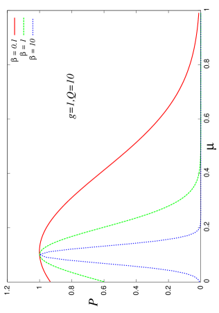
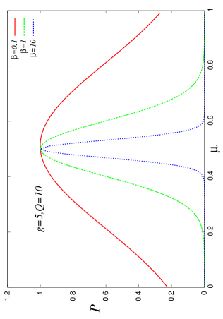
Figure 11: The distribution $P_{\mu,Q}(\mu)$ for several values of $Q$ and $\beta$ and $g$.

From this figure, we find that as temperature $\beta^{-1}$ decreases, the distribution changes its shape to the delta function in which the peak is located at $g_{0}/Q$. This means that simulated annealing safely finds the ground state of the Hamiltonian having the zero energy, namely,

$$\forall_{i}\,\,\,\,\,\,g_{0}=g_{i} = \sum_{k\in\mathbb{N}(i)}\Theta(g_{k}-t_{k})=s_{i}$$ (102)

This immediately reads $\mu_{i}=g_{0}/Q$ for all index $i$. Therefore, for a given image having a single grayscale $g_{0}$, the distribution should converge to the delta function with the peak at $g_{0}/Q$ if the annealing schedule of $\beta$ is appropriate.

Appendix B Inverse halftoning as an ill-posed problem

Here we shall consider the inverse process of halftoning as an ill-posed problem. In the inverse halftoning, we should solve $\forall_{x,y}\,\,\,h_{x,y}=\Theta(g_{x,y}-t_{x,y})$ with respect to $g$ for a given halftoned image $h$ and the mask $t$. Obviously, this problem is ill-posed because there are a lot of candidates to satisfy the equations. In this Appendix, we analytically evaluate several relevant quantities to show the difficulty in finding the solution.

B.1 Degree of degeneracy for possible solutions

We easily assume that the number of the solutions for a given $h$ and $t$ is exponential order, however, it is helpful for us to evaluate the number more precisely. For the purpose, let us use the definition introduced in the previous section, namely, $i=x+Ly-L,i=1,2,\cdots,L^{2}\equiv N$ (conversely, $x=(i\mod L),y=[i/L]$). Then, the number of the candidates for the solution of the equations $\forall_{i}\,\,\,h_{i}=\Theta(g_{i}-t_{i})$ is evaluated for a given a realization of the original image and the threshold mask as follows.

$$\mathcal{N}(\mbox{\boldmath$g$},\mbox{\boldmath$t$}) = \prod_{i=1}^{N}\left\{(Q-1-t_{i})\Theta(g_{i}-t_{i})+t_{i}\Theta(t_{i}-g_{i})\right\}$$ (103)

As the number $\mathcal{N}$ seems to be an exponential order object, we might rewrite the data average of the logarithm of the number as a self-averaging quantity

$$\mathbb{E}_{\mbox{\scriptsize\boldmath$g$},\mbox{\scriptsize\boldmath$t$}}[\log\mathcal{N}(\mbox{\boldmath$g$},\mbox{\boldmath$t$})] = \mathbb{E}_{\mbox{\scriptsize\boldmath$g$},\mbox{\scriptsize\boldmath$t$}}\left[\log\prod_{i=1}^{N}\left\{(Q-1-t_{i})\Theta(g_{i}-t_{i})+t_{i}\Theta(t_{i}-g_{i})\right\}\right]$$ (104)

where we defined the expectation $\mathbb{E}_{\mbox{\scriptsize\boldmath$g$},\mbox{\scriptsize\boldmath$t$}}[\cdots]$ by

$$\mathbb{E}_{\mbox{\scriptsize\boldmath$g$},\mbox{\scriptsize\boldmath$t$}}[\cdots] \equiv \int\int P_{J_{0}}(\mbox{\boldmath$g$})P(\mbox{\boldmath$t$})(\cdots)d\mbox{\boldmath$g$}\,d\mbox{\boldmath$t$},\,\,\,d\mbox{\boldmath$g$}\equiv\prod_{i=1}^{N}dg_{i},\,d\mbox{\boldmath$t$}\equiv\prod_{i=1}^{N}dt_{i}.$$ (105)

Therefore, the above averages could be carried out for a specific choice of the $P(\mbox{\boldmath$g$})$ and $P(\mbox{\boldmath$t$})$. For distributions of the threshold mask, we suppose that in each mask with size $Q\times Q$ ($Q\ll N$), each component $t_{i}$ takes a value among $0,\cdots,Q-1$ grayscales with equal probability $1/Q$. Then, the $P(\mbox{\boldmath$t$})$ is reduced to the product of the effective single site distribution as

$$P(\mbox{\boldmath$t$})=\prod_{i=1}^{N}P(t_{i}) = \frac{1}{Q}\prod_{i=1}^{N}\sum_{l_{i}=0}^{Q-1}\delta_{l_{i},t_{i}}.$$ (106)

On the other hand, as a distribution of the original image, we consider snapshots from the infinite-range ferromagnetic Q-Ising model, that is,

$$P_{J_{0}}(\mbox{\boldmath$g$}) = \frac{\exp(-\mathcal{H})}{Z_{0}},\,\,\,\,\mathcal{H}=\frac{J_{0}}{2N}\sum_{ij}(g_{i}-g_{j})^{2}$$ (107)

where $Z_{0}$ is a normalization constant for the probability $P_{J_{0}}(\mbox{\boldmath$g$})$. After simple algebra, we find that the $P_{J_{0}}(\mbox{\boldmath$g$})$ is rewritten such as $P_{J_{0}}(\mbox{\boldmath$g$})=\prod_{i=1}^{N}P_{J_{0}}(g_{i})$ with the following effective single site distribution:

$$P_{J_{0}}(g_{i}) = \frac{\exp(-J_{0}g_{i}^{2}+2J_{0}m_{0}g_{i})}{\sum_{g_{i}=0}^{Q-1}\exp(-J_{0}g_{i}^{2}+2J_{0}m_{0}g_{i})},\,\,\,\,m_{0}=\frac{\sum_{g=0}^{Q-1}g\,\exp(-J_{0}g^{2}+2J_{0}m_{0}g)}{\sum_{g=0}^{Q-1}\exp(-J_{0}g^{2}+2J_{0}m_{0}g)}$$ (108)

where $m_{0}=(1/N)\sum_{i=1}^{N}g_{i}$ denotes the magnetization for the system of original grayscale images described by the Hamiltonian (107). For these probability distributions, we have the function $\phi(J_{0},Q)\equiv N^{-1}\mathbb{E}_{\mbox{\scriptsize\boldmath$g$},\mbox{\scriptsize\boldmath$t$}}[\log\mathcal{N}(\mbox{\boldmath$g$},\mbox{\boldmath$t$})]$ explicitly as

$$\phi(J_{0},Q) = \sum_{g,t=0}^{Q-1}P_{J_{0}}(g)P(t)\log\left\{(Q-1-t)\Theta(g-t)+t\Theta(t-g)\right\}$$ (109)

$$= \frac{\sum_{t=0}^{Q-1}\sum_{l=0}^{Q-1}\delta_{l,t}\sum_{g=0}^{Q-1}{\rm e}^{-J_{0}g^{2}+2J_{0}m_{0}g}\log\left\{(Q-1-t)\Theta(g-t)+t\Theta(t-g)\right\}}{Q\sum_{g=0}^{Q-1}{\rm e}^{-J_{0}g^{2}+2J_{0}m_{0}g}}.$$

Therefore, the number of the solutions for the equations $\forall_{i}\,\,\,h_{i}=\Theta(g_{i}-t_{i})$ is estimated as $\sim\exp(N\phi(J_{0},Q))$. In FIG. 12, we plot the function $\phi(J_{0},3)$ and $\phi(J_{0},4)$.

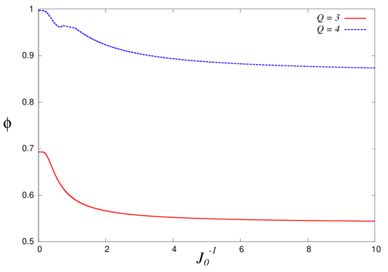
Figure 12: Logarithm of the number of candidates (degeneracy) for the solutions $\phi$ as a function of $J_{0}^{-1}$ for $Q=3$ and $4$.

From this figure, we find that the $\phi$ is a monotonically decreasing function as $J_{0}^{-1}$ decreases, however, the $\phi$ remains a finite value even if $J_{0}^{-1}\to\infty$. This means that the number of the candidates for the solutions of the inverse halftoning is always exponential order. Therefore, we need some systematic approach to solve this type of the ill-posed problems. Namely, we need to introduce the ferromagnetic prior $P_{J}(\mbox{\boldmath$\sigma$})$ to compensate the lack of information as we discussed in Sec. IV.

B.2 Mutual information

We next consider the difficulties of retrieving original grayscale images from a slightly different point of view. Here we calculate the mutual information between the original image $g$ and the halftone image $h$. From the definition of the mutual information, we should evaluate $I(\mbox{\boldmath$g$}:\mbox{\boldmath$h$})=H(\mbox{\boldmath$h$})-H(\mbox{\boldmath$h$}|\mbox{\boldmath$g$})$, where we defined the entropy $H(\mbox{\boldmath$h$})$ and the conditional entropy $H(\mbox{\boldmath$h$}|\mbox{\boldmath$g$})$ as $H(\mbox{\boldmath$h$})=-\sum_{\mbox{\scriptsize\boldmath$h$}}P(\mbox{\boldmath$h$})\log P(\mbox{\boldmath$h$}),H(\mbox{\boldmath$h$}|\mbox{\boldmath$g$})=-\sum_{\mbox{\scriptsize\boldmath$g$}}P_{J_{0}}(\mbox{\boldmath$g$})\sum_{\mbox{\scriptsize\boldmath$h$}}P_{t}(\mbox{\boldmath$h$}|\mbox{\boldmath$g$})\log P_{t}(\mbox{\boldmath$h$}|\mbox{\boldmath$g$})$, respectively. It should be noted that we used

$$P_{t}(\mbox{\boldmath$h$}|\mbox{\boldmath$g$}) = \prod_{i}\delta(h_{i},\Theta(g_{i}-t_{i}))$$ (110)

and $P(\mbox{\boldmath$h$})=\sum_{\mbox{\scriptsize\boldmath$g$}}P_{t}(\mbox{\boldmath$h$}|\mbox{\boldmath$g$})P_{J_{0}}(\mbox{\boldmath$g$})$.

For the infinite-range model and constant mask $t_{i}=t_{0}\,\,\,\forall_{i}$, these entropies per are calculated analytically as

$$\frac{H(\mbox{\boldmath$h$})}{N} = -\sum_{h=0,1}\sum_{g=0}^{Q-1}\left\{\frac{{\rm e}^{-J_{0}g^{2}+2J_{0}m_{0}g}\delta(h,\Theta(g-t_{0}))}{Z_{J_{0}}}\right\}\log\left\{\frac{\sum_{g=0}^{Q-1}{\rm e}^{-J_{0}g^{2}+2J_{0}m_{0}g}\delta(h,\Theta(g-t_{0}))}{Z_{J_{0}}}\right\}$$ (111)

$$\frac{H(\mbox{\boldmath$h$}|\mbox{\boldmath$g$})}{N} = -\sum_{g=0}^{Q-1}\left\{\frac{{\rm e}^{-J_{0}g^{2}+2J_{0}m_{0}g}}{Z_{J_{0}}}\right\}\sum_{h=0,1}\delta(h,\Theta(g-t_{0}))\log\delta(h,\Theta(g-t_{0}))=0$$ (112)

where we defined $Z_{J_{0}}\equiv\sum_{g=0}^{Q-1}{\rm e}^{-J_{0}g^{2}+2J_{0}m_{0}g}$ and $m_{0}$ is a solution of the equation (108). We should keep in mind that the ‘channel’ of the halftoning process is completely deterministic. As the result, the conditional entropy $H(\mbox{\boldmath$h$}|\mbox{\boldmath$g$})$ is identically zero. In FIG. 13, we plot the mutual information per pixel $I(\mbox{\boldmath$g$}:\mbox{\boldmath$h$})/N$ as a function of $J_{0}$.

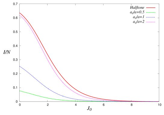
Figure 13: The mutual information per pixel as a function of $J_{0}$. For the halftoning process, we choose $Q=3$ and $t_{0}=1$. The mutual information for image restoration under Gaussian noise is also plotted for the signal to noise ratio $a_{0}/a=0.5,1$ and $2$.

To compare halftoning process by the dither method with the degraded process by a Gaussian noise with mean $a_{0}g$ and the variance $a^{2}$, we also calculate the mutual information per pixel for the Gaussian noise. We choose the same distribution $P_{J_{0}}(\mbox{\boldmath$g$})$ as the halftone case. We immediately have

$$\frac{H(\mbox{\boldmath$h$})}{N} = -\frac{1}{\sqrt{2\pi}aZ_{J_{0}}}\int_{-\infty}^{\infty}dh\sum_{g=0}^{Q-1}{\rm e}^{-J_{0}g^{2}+2J_{0}m_{0}g-\frac{(h-a_{0}g)^{2}}{2a^{2}}}\log\left\{\frac{\sum_{g=0}^{Q-1}{\rm e}^{-J_{0}g^{2}+2J_{0}m_{0}g-\frac{(h-a_{0}g)^{2}}{2a^{2}}}}{\sqrt{2\pi}aZ_{J_{0}}}\right\}$$ (113)

$$\frac{H(\mbox{\boldmath$h$}|\mbox{\boldmath$g$})}{N} = \frac{1}{2}+\log(\sqrt{2\pi}a).$$ (114)

In FIG. 13, we plot the mutual information per pixel for the Gaussian noise as a function of $J_{0}$ for various cases of the signal-noise ratio, $a_{0}/a$.

References

- (1) M. Mézard M, G. Parisi and M.A. Virasoro, Spin Glass Theory and Beyond (Singapore: World Scientific) (1987).
- (2) H. Nishimori, Statistical Physics of Spin Glasses and Information Processing: An Introduction (Oxford: Oxford University Press) (2001).
- (3) C. M. Bishop, Pattern Recognition and Machine Learning, (Singapore: Springer) (2006).
- (4) M. Mézard and A. Montanari, Information, Physics, and Computation, Oxford University Press (2009).
- (5) N. Sourlas, Nature 339, 693 (1989).
- (6) P. Rujn, Phys. Rev. Lett. 70 2968 (1993).
- (7) Y. Kabashima and D. Saad, Europhys. Lett. 45 98 (1999).
- (8) T. Tanaka, Europhys. Lett. 54 (4), 540 (2001).
- (9) K. Tanaka, J. Phys. A: Math. Gen. 35 R81 (2002).
- (10) D.L. Lau and G.R. Ace, Modern digital halftoning, Marcel Dekker, Ink (2001).
- (11) R. Ulichney, Digital Halftoning, The MIT Press (1987).
- (12) M. Analoui and J.P. Allebach, Proceedings SPIE, Human Vision, Visual Processing, and Digital Display III 1666, 96 (1992).
- (13) J.L. Mannos and D.J. Sakrison, IEEE Trans. Information Theory IT-20, 525 (1974).
- (14) T. Mista and K.J. Parker, J. Opt. Soc. Am. A9, 1920 (1992).
- (15) R.A. Ulichney, Proceedings of the IEEE 76, 56 (1988).
- (16) R.W. Floyd and L. Steinberg, Proceedings Society Information Display 17, 75 (1976).
- (17) J. Inoue and Y. Saika and M. Okada, Proceedings of 7th International conference on Intelligent Systems Design and Applications (ISDA07), 617 (2007).
- (18) Y. Saika, J. Inoue, H. Tanaka and M. Okada, Central European Journal of Physics 7, pp. 444-456 (2009).
- (19) S. Kirkpatrick, C.D. Gellet and M.P. Vecci, Science 220, 671 (1983).
- (20) S. Geman and D. Geman, IEEE Transaction on Pattern Analysis and Machine Intelligence 6, 721 (1984).
- (21) H. Nishimori, Prog. Theor. Phys. 66 1169 (1981).
- (22) T.N. Pappas and D.L. Neuhoff, Proceedings of SPIE, Human Vision, Visual Processing, and Digital Display III 1666 96 (1992).
- (23) T.N. Pappas, IST’s 8th International Congress on Advances in Non-Impact Printing Technologies, 270 (1992).
- (24) T.N. Pappas, International Journal of Imaging Systems and Technology 7, 110 (1996).
- (25) T. Tadaki and J. Inoue, Phys. Rev. E 65, 016101 (2002).