Wavelets with ridges: a high-resolution representation of cataclysmic variable time-series

Abstract

Quasi-periodic oscillations and dwarf nova oscillations occur in dwarf novae and nova-like variables during outburst and occasionally during quiescence, and have analogues in high-mass X-ray binaries and black-hole candidates. The frequent low coherence of quasi-period oscillations and dwarf nova oscillations can make detection with standard time-series tools such as periodograms problematic. This paper develops tools to analyse quasi-periodic brightness oscillations. We review the use of time-frequency representations in the astronomical literature, and show that representations such as the Choi-Williams Distribution and Zhao-Atlas-Marks Representation, which are best suited to high signal-to-noise data, cannot be assumed a priori to be the best techniques for our data, which have a much higher noise level and lower coherence. This leads us to a detailed analysis of the time-frequency resolution and statistical properties of six time-frequency representations. We conclude that the wavelet scalogram, with the addition of wavelet ridges and maxima points, is the most effective time-frequency representation for analysing quasi-periodicities in low signal-to-noise data, as it has high time-frequency resolution, and is a minimum variance estimator.

We use the wavelet ridges method to re-analyse archival data from VW Hyi, and find 62 new QPOs and 7 new long-period DNOs. Relative to previous analyses, our method substantially improves the detection rate for QPOs.

1 Introduction

Cataclysmic variable (CV) light curves frequently contain multiple (quasi-)periodic components covering a wide frequency range, from 3 s dwarf nova oscillations (DNOs) (Woudt & Warner, 2002a) through $\sim$100 s longer period DNOs (lpDNOs) (Warner, Woudt & Pretorius, 2003) to $\sim$5000 s quasi-periodic oscillations (QPOs) (Patterson et al., 1977). Each of these components can vary in period, amplitude and phase on short time-scales, against a high level of background noise. DNOs, with $Q=|\frac{dP}{dt}|^{-1}\approx 10^{4}-10^{6}$, are generally more coherent than QPOs ($Q\approx 1-10$), but both are seldom visible directly in the light curve, and the periodogram, which is designed for stationary phenomena, can fail to detect them (see for example Robinson & Nather, 1979). Thus in order to study these and similar phenomena it is important to find a tool that detects them reliably. An investigation of time-frequency representations, which allow a non-stationary signal to be visualized in the time and frequency domains simultaneously, and have been successfully used in other areas of astronomy, would seem to be an intuitive and instructive place to begin.

The most common time-frequency representation in use in astronomy is the wavelet transform, either in the form of the weighted wavelet Z-transform (WWZ) of Foster (1996) or the wavelet scalogram. We will focus on the wavelet scalogram as our data are regularly spaced, and the WWZ is designed for irregularly spaced data and has poorer time-frequency resolution. The wavelet scalogram has been used to analyse, amongst other astronomical phenomena, SR-type stars (Chinarova & Andronov, 2000; Kiss, Szabó & Bedding, 2006), CVs (Fritz & Bruch, 1998; Halevin et al., 2002) and planetary nebulae (González Pérez et al., 2003). The significance testing method of Torrence & Compo (1998) for the wavelet scalogram is used mainly in solar astrophysics, where it has been applied to magnetic field measurements (Boberg & Lundstedt, 2002), coronal variability (Marsh, Walsh & Bromage, 2002), high-frequency oscillations in coronal loops (Katsiyannis et al., 2002) and chromospheric UV oscillations (McAteer et al., 2004).

Several other time-frequency representations have also been used in astronomy. The Gabor spectrogram has been applied to synthetic multi-component signals and roAP stars (Boyd et al., 1995) and QPOs in both the atoll source 4U 1820-30 (Belloni, Parolin & Casella, 2004) and Her X-1 (O’Brien et al., 2001). The Choi-Williams distribution was applied to Wolf-Rayet stars (Marchenko & Moffat, 1998) and the Cone-Kernel Representation to irregular pulsators (Buchler, Kolláth & Cadmus, 2004) and T UMi (Szatmary, Kiss & Bebesi, 2003).

There are several key differences between our data and those analysed in the literature which make the choice of the most appropriate time-frequency representation for our analysis unclear. Firstly, in all of the papers mentioned above (and, indeed, all those in the literature) either visual inspection of the light curve or calculation of the periodogram is the primary source of periodicity detection; the time-frequency representation serves merely as an adjunct. For our signals, which have lower signal-to-noise ratios than those in the literature and which cannot be seen directly in the light curve or the periodogram, the time-frequency representation will be the primary means of detection, and hence it is imperative that we be able to test the significance of any detections statistically. Apart from Boyd et al. (1995), the only papers conducting significance testing of time-frequency representations are those using the Torrence & Compo (1998) wavelet scalogram method.

Our analysis also requires a broader frequency range than any discussed in the literature, as well as very high frequency resolution, particularly in the QPO frequency range as QPOs often appear as closely spaced harmonics. In addition, since both DNOs and QPOs are intermittent phenomena that can change their characteristics on a time-scale of 10 s of seconds, we need high time resolution over the entire frequency range. Thus time-frequency representations with higher time-frequency resolution would be preferable for our analysis. Comparisons of the wavelet scalogram, Gabor spectrogram, Choi-Williams distribution and the Cone-Kernel Representation show that, at least for relatively large amplitude variables stars such as irregular pulsators or Mira-types, the Choi-Williams distribution and Cone-Kernel Representation can give better time-frequency resolution than the wavelet scalogram (e.g. Kolláth & Buchler, 1997; Buchler & Kolláth, 2001; Kiss & Szatmáry, 2002).

A plethora of papers investigate the effectiveness of different time-frequency representations using various synthetic signals (see for example Goupil, Auvergne & Baglin (1991), Carothers & Swenson (1992), Szatmary, Vinko, & Gál (1994), Boyd et al. (1995), Li, Jia & Zhao (1999), Hlawatsch et al. (1995), Buchler & Kolláth (2001), Kiss & Szatmáry (2002), Thayaparan & Kennedy (2003), Szatmary, Kiss & Bebesi (2003) or Figueiredo et al. (2004)), but as none of these synthetic data have features comparable to those of our data we cannot necessarily use their conclusions.

Section 2 gives a brief introduction to the Wigner-Ville Distribution, and explains why the interference terms which distort this time-frequency representation have resulted in the development of a large number of alternative representations. In section 3 we analyse the time-frequency resolution and statistical properties of six of these alternative time-frequency representations using three synthetic (noise-free) signals mimicking key features of our data. We conclude that the Morlet wavelet scalogram, with the addition of wavelet ridges and maxima lines is the optimal choice for our data, both in terms of its time-frequency resolution and statistical properties. We use this representation to re-analyse archival data of VW Hyi in section 4, and show that it does indeed provide a reliable tool for detecting QPOs, with a significantly higher detection rate than previous methods. Section 5 concludes.

2 A brief introduction to time-frequency representations

The archetypal time-frequency representation (TFR) of a signal $x(t)$ is the Wigner-Ville Distribution (WVD), given by

$$W_{x}(t,f)=2\int_{-\infty}^{+\infty}x(t+\tau)x^{*}(t-\tau)e^{4\pi f\tau i}d\tau$$ (1)

(Ville, 1948).

In practise, for finite duration signals, the pseudo Wigner-Ville distribution (PWVD), given by

$$W_{x}(t,f)=2\int_{-\infty}^{+\infty}h(\tau)x(t+\tau)x^{*}(t-\tau)e^{4\pi f\tau i}d\tau.$$ (2)

is used, where $h(t)$ is a rectangular window that is zero outside the duration of the signal. If $x(t)$ is sampled at times $t=0,\Delta t,2\Delta t,...$ then, in order to prevent spectral aliasing in the WVD and PWVD, either the signal must be oversampled by a factor of at least 2, or the analytic signal (Auger et al., 1996). The analytic version $x_{a}(t)$ of a signal $x(t)$ is the inverse Fourier transform of

$$\hat{x}_{a}(f)=\left\{\begin{array}[]{ll}2\hat{x}(f)&\mbox{if $f\geq 0$}\\ 0&\mbox{if $f<0$}\end{array}\right.$$ (3)

We assume throughout the rest of the paper that the analytic signal is used.

Ville originally investigated TFRs in order to study the instantaneous frequency of signals with time-varying components. A real (mono-component) signal $x(t)$ may be written as a time varying amplitude $a(t)$ modulated by a time varying phase $\phi$:

$$x(t)=a(t)\cos[\phi(t)]$$ (4)

with $a(t)\geq 0$. The instantaneous (angular) frequency is then defined as the positive derivative of the phase:

$$\omega(t)=\phi^{\prime}(t)\geq 0$$ (5)

(Gonçalves et al., 1997). Since there are many possible choices of $a(t)$ and $\phi(t)$ for any given signal, $\omega(t)$ is not uniquely defined. However, using the analytic signal, we have $x_{a}(t)=a(t)\exp[i\phi(t)]$ and, since $x(t)=\mathrm{Re}[x_{a}(t)]$, then $x(t)=a(t)\cos\phi(t)$. We call $a(t)$ the analytic amplitude of $x(t)$ and $\phi^{\prime}(t)$ its instantaneous frequency (Mallat, 1998). Multicomponent signals in which the components occur in disjoint frequency bands can be thought of as the sum of mono-component signals; it is the aim of the TFR to show the instantaneous frequency of each component accurately.

Figure 1(a) shows the time-series of a synthetic signal which mimics a noise-free dwarf nova (DN) lightcurve sampled with an integration time of 4 s, with a first harmonic DNO changing linearly in period from 25 s to 30 s over the duration of the run, fundamental and first harmonic QPOs starting with periods 750 s and 375 s respectively and tracking the period change of the DNO, and an lpDNO with a constant 70 s period, based on run s0484 of VW Hyi, discussed in Woudt & Warner (2002a). An idealised TFR (Figure 1(b)) and the PWVD (Figure 1(c)) are shown below the time-series.

Figure 1: (a) Time-series of a synthetic signal which mimics a noise-free dwarf nova (DN) lightcurve, with a first harmonic DNO changing linearly in period from 25 s to 30 s, fundamental and first harmonic QPOs starting with periods 750 s and 375 s respectively and tracking the period change of the DNO, and an lpDNO with a constant 70 s period. (b) Idealised TFR of the signal in Figure 1(a). (c) WVD of the signal in Figure 1(a)

While the changing DNO and QPO periodicities are clearly visible in the PWVD in Figure 1(c), as is the constant period lpDNO, there are also five sets of spurious signals, called interference terms (ITs), which are an artefact of the quadratic nature of the WVD. The WVD of an N-component signal will always consist of N signal terms and $\frac{N(N-1)}{2}$ ITs (Mecklenbräuker & Hlawatsch, 1997). ITs oscillate in the time and frequency directions (Hlawatsch & Urbanke, 1994), and the closer together two components are in frequency, the slower their ITs will oscillate in the time direction (Hlawatsch & Boudreaux-Bartels, 1992). This is clear in figure 1(c): the ITs due to the interaction between the two close QPO terms oscillate much more slowly in the time direction than the ITs due to the other interactions, whose generating signal terms are further apart in frequency.

The presence of ITs in the WVD make it unsuitable for analysis of data in which the true signal components are unknown, or cannot be inferred by other means - as is the case for our data. However, since the ITs are oscillatory, they can be reduced or removed entirely by smoothing the WVD in the time and frequency directions. IT attenuation is usually achieved by convolving the WVD with a 2-D smoothing kernel (Hlawatsch & Boudreaux-Bartels, 1992).

IT reduction comes at a cost: the more smoothing in time and/or frequency, the poorer the resolution in time and/or frequency (Cohen, 1989). The WVD has the best possible time-frequency resolution of all TFRs: for a time-dirac signal centered at $t_{0}$, $W_{x}(t,f)=\delta(t-t_{0})$ , and for a frequency dirac signal centered at $f_{0}$, $W_{x}(t,f)=\delta(f-f_{0})$ (Mallat, 1998). All other TFRs generally have poorer time and frequency resolution, or may achieve that of the WVD for certain types of signal only.

Since the geometry of the ITs depends on the components of the signal, different smoothing kernels have been developed for different kinds of signals: there is no single kernel which is optimal for all signals. Most kernels however belong to the Cohen class (Cohen, 1989) or the affine class (Rioul & Flandrin, 1992) or both, and have one or more parameters which can be varied to choose the amount of smoothing in time and/or frequency.

The Cohen TFRs (Cohen, 1989), which we will denote generally as $C_{x}(t,f)$, are derived from a time-frequency convolution of the WVD with a smoothing kernel $\psi(t,f)$:

$$C_{x}(t,f)=\int_{t^{\prime}}\int_{f^{\prime}}\psi(t-t^{\prime},f-f^{\prime})W_{x}(t^{\prime},f^{\prime})dt^{\prime}df^{\prime}$$ (6)

or, more traditionally, as

$$C_{x}(t,f)=\int_{\tau}\int_{\nu}\Psi(\tau,\nu)\Lambda_{x}(\tau,\nu)e^{i2\pi(t\nu-f\tau)}d\tau d\nu$$ (7)

where $\Psi(\tau,\nu)$ is the Fourier transform of $\psi(t,f)$ and $\Lambda_{x}(\tau,\nu)$ is the ambiguity function (AF) of $x(t)$, defined as:

$$\begin{array}[]{ll}\Lambda_{x}(\tau,\nu)&=2\int_{t}x(t+\tau)x^{*}(t-\tau)e^{-i4\pi\nu t}dt\\ &=2\int_{f}\hat{x}(f+\nu)\hat{x}^{*}(f-\nu)e^{i4\pi\tau f}df.\\ \end{array}$$ (8)

Here $\tau$ is the time-delay, and $\nu$ is the Doppler value, which measures the difference in frequencies between points at a given time-delay (Hlawatsch et al., 1995). The AF, which is the Fourier transform of the WVD, can be interpreted as a joint time-frequency correlation function (Hlawatsch & Boudreaux-Bartels, 1992).

Each member of Cohen’s class is thus associated with a unique, signal independent kernel function $\Psi(\tau,\nu)$; the WVD is a member of the Cohen class, with kernel $\Psi_{WVD}(\tau,\nu)=1$.

The general affine TFR ($A_{x}(t,a;\Pi)$) of an analytic signal $x(t)$ is given by

$$A_{x}(t,a;\Pi)=\int_{-\infty}^{\infty}\int_{-\infty}^{\infty}\Pi(\frac{s-t}{a},a\xi)W_{x}(s,\xi)dsd\xi$$ (9)

where $\Pi(t,\nu)$ is a smoothing kernel. Equivalently, using the AF instead of the WVD, we have

$$A_{x}(t,a;\Psi)=\int_{-\infty}^{\infty}\int_{-\infty}^{\infty}\Psi(a\xi,\tau/a)\Lambda_{x}(\xi,\tau)e^{-i2\pi\xi t}d\xi d\tau$$ (10)

where $\Psi(\xi,\tau)$ is the ambiguity domain version of $\Pi(t,\nu)$. Affine TFRs are time-scale representations rather than time-frequency representations, but $a$ acts as a measure of the frequency: reducing $a$ reduces the time support of $\Pi_{t,s}$, and hence increases its frequency range (Goswami & Chan, 1999). Since the WVD is scale-invariant, it is also a member of the affine class.

In both Cohen and affine TFRs, the kernel determines the amount of smoothing in time and/or frequency. The important difference between affine and Cohen TFRs is that the affine kernel is scaled depending on the analysing frequency, while Cohen kernels retain the same ‘size’ at all frequencies. This means that for affine TFRs the time and frequency resolutions depend on the frequency at which the signal is being analysed, while for Cohen TFRs the time and frequency resolutions are the same at all frequencies.

Table 1: TFR kernels and their properties

Name	Kernel $\Psi(\tau,\nu)$	Parameter(s)	Cohen	Affine	Statistics
Wigner-Ville (WVD)	1	-	✓	✓	$S_{noise}(f)\frac{\chi_{2}^{2}}{2}$
Smoothed Pseudo Wigner-Ville (SPWVD)	$g(\frac{\tau}{2})g^{*}(-\frac{\tau}{2})\hat{h}(\nu)$	$L_{g}$, $L_{h}$	✓		$\frac{2}{2M-1}S_{noise}(f)\frac{\chi_{2}^{2}}{2}$
Choi-Williams (CWD)	$e^{-\frac{(2\pi\tau\nu)^{2}}{\sigma}}$	$\sigma$	✓		$S_{noise}(f)\frac{\chi_{2}^{2}}{2}$
Born-Jordan (BJD)	$\frac{\sin(\pi\tau\nu)}{\pi\tau\nu}$	-	✓		$S_{noise}(f)\frac{\chi_{2}^{2}}{2}$
Cone-Kernel (CKR)	$g(\tau)|\tau|\frac{\sin(\pi\tau\nu)}{\pi\tau\nu}$	$L_{g}$	✓		$S_{noise}(f)\frac{\chi_{2}^{2}}{2}$
Affine Smoothed Pseudo Wigner-Ville (ASPWVD)	$h(\frac{\tau}{a})g(\frac{s-\tau}{a})$	$L_{g}$, $L_{h}$		✓	$\frac{2}{2M_{s}-1}S_{noise}(s)\frac{\chi_{2}^{2}}{2}$
Gabor Spectrogram (SPEC)	$W_{h}(-\tau,-\nu)$	$L_{h}$	✓		$S_{noise}(f)\frac{\chi_{2}^{2}}{2}$
Scalogram (SCALO)	$W_{\psi}(\tau,\nu)$	$L_{\psi}$		✓	$S_{noise}(f)\frac{\chi_{2}^{2}}{2}$

3 Six smoothing kernels investigated

We will investigate 4 Cohen and 2 affine smoothing kernels which have either been previously used in used in astronomy or have properties which suggest they are appropriate for our data; Table 1 gives a summary of the main features of the kernels discussed. We begin our analysis by finding the optimal parameters needed for each TFR in order to represent the synthetic DN lightcurve introduced in section 2 without interference terms. This signal tests the frequency resolution of each TFR over a broad frequency range, and ensures that the values of the parameters chosen completely attenuate interference terms over the whole frequency range. Using these optimal parameters, we then further investigate the time resolution of each TFR by using intermittent sinusoids of different frequencies. Where possible, we include a discussion the use of the kernel in the astronomical literature. We conclude this section with a discussion of the statistical properties of the six kernels.

3.1 The Smoothed Pseudo WVD

One method of smoothing the WVD is to use the separable kernel

$$\Psi_{SPWVD}(\tau,\nu)=g(\frac{\tau}{2})g^{*}(-\frac{\tau}{2})\hat{h}(-\nu)$$ (11)

with time-smoothing window $g(t)$ and frequency-smoothing window $\hat{h}(\nu)$ (which is the Fourier transform of a time-smoothing window $h(t)$) (Auger et al., 1996). The length $L_{g}$ ($L_{h}$) of the window $g(t)$ ($h(t)$) controls the amount of smoothing in the time (frequency) domain. A longer $g(t)$ gives more time smoothing and hence worse time resolution, and a longer $h(t)$ gives less frequency smoothing and hence better frequency resolution (Hlawatsch et al., 1995).

Figures 2 and 3 show the smoothed pseudo WVD (SPWVD) of the synthetic DN lightcurve, with $L_{g}=$ 200 s in both figures, but $L_{h}=$ 200 s in the first, and $L_{h}=$ 1200 s in the second. The effect of increasing $L_{h}$ (i.e. decreasing the frequency smoothing) is marked: in the first figure, we cannot differentiate the two long period QPO components, but in the second they are clearly visible. Interference terms between the two long-period components in Figure 3 are still prominent. By increasing $L_{g}$ to 1000 s, as in figure 4, the interference terms are completely attenuated. Notice, however, the effect of the extensive time smoothing at the ends of the DNO.

Next, we use these optimal values of $L_{g}$ and $L_{h}$ to investigate an intermittent sinusoid of period 100 s, shown figure 5(a), mimicking for example an intermittent lpDNO. The integration time is 4 s.

The time-smoothing introduced by increasing $L_{g}$, which was necessary to attenuate the ITs, has come at a price: the ability of the SPWVD to clearly resolve temporal discontinuities in the signal. In figure 5(b) the smoothing in the time domain results in a SPWVD that does not clearly show the beginning or end of each sinusoidal burst. Indeed, it gives the impression that the sinusoid is perhaps present for the duration of the signal, but at varying amplitude. There are two reasons for this: signal terms, which should not be smoothed, are smeared in the time dimension by the long time window, and ITs which oscillate in the frequency direction between the signal terms are not removed because we have set the length of the frequency smoothing window to ensure that we have optimal frequency resolution (i.e. minimal smoothing).

We are thus presented with the central issue that dogs most Cohen kernels: if ITs are attenuated by smoothing in time, the result is poor time resolution, which is particularly problematic at high frequencies.

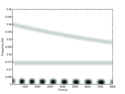
Figure 2: Smoothed Pseudo Wigner-Ville distribution of synthetic DN lightcurve, with L${}_{g}=$200s, L${}_{h}=$200.

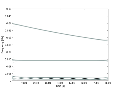
Figure 3: Smoothed Pseudo Wigner-Ville distribution of the synthetic DN lightcurve, with L${}_{g}=$200s, L${}_{h}=$1200s.

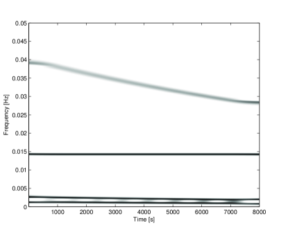
Figure 4: Smoothed Pseudo Wigner-Ville distribution of the synthetic DN lightcurve, with L${}_{g}=$1000s, L${}_{h}=$1200s.

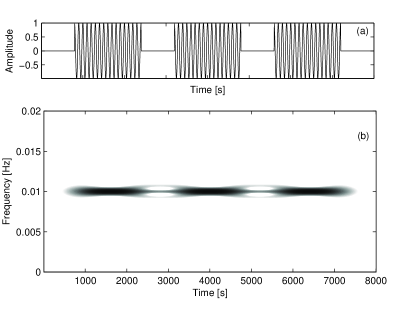
Figure 5: Smoothed Pseudo Wigner-Ville distribution of an intermittent sinusoid of period 100 s, with L_g 1000s, L_h 1200s.

3.2 The Affine Smoothed Pseudo WVD

The affine smoothed pseudo WVD (ASPWVD) is the affine counterpart of the SPWVD, and its kernel is given by

$$\Psi_{ASPWVD}=h(\frac{\tau}{a})g(\frac{s-t}{a}),$$ (12)

where $g(t)$ and $h(t)$ are smoothing windows as for the SPWVD. The lengths of the time and frequency smoothing windows, $L_{g}$ and $L_{h}$ respectively, again allow a flexible choice of time and scale (frequency) resolution.

Figures 6 and 7 show the ASPWVD of the synthetic DN lightcurve, with $L_{g}$ set to 0 s in the first case (no time smoothing) and 320 s (at the largest scale) in the second. $L_{h}$ is 320 s in both cases, which is the minimum length needed to resolve both QPOs. What is apparent in Figure 7, when compared with the SPWVD shown in Figure 4, is that less time smoothing is needed to remove the ITs in the ASPWVD, resulting in less noticeable end-effects. However, the frequency resolution decreases in the ASPWVD as the frequency increases, so the DNO in the ASPWVD is broader than the DNO in the PSWVD.

In comparison with the SPWVD, the ASPWVD of the intermittent sinusoid, shown in figure 8, has good time resolution (since for affine distributions the time resolution improves as the frequency increases), but has poorer frequency resolution than the SPWVD. No ITs are visible between the bursts of signal.

The top panel of figure 9 shows a signal mimicking an intermittent 20 s DNO with changing amplitude, sampled with an integration time of 4 s. The ASPWVD of this signal, calculated using $L_{g}=L_{h}=$ 320 s is shown in the bottom panel. Very broadly smoothed signal terms and ITs considerably distort the true signal, and it is not possible to remove these interference terms without losing the optimal resolution achieved for the analysis of the DN signal.

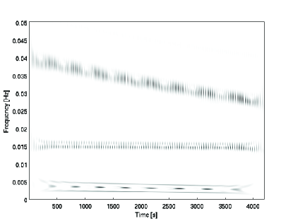
Figure 6: ASPWVD of the synthetic DN lightcurve, with $L_{g}=0$s and $L_{h}=320s.$

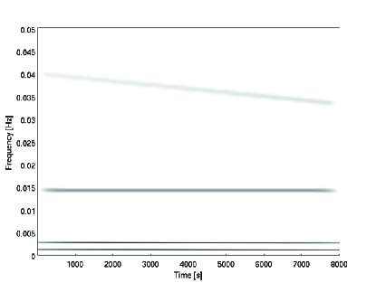
Figure 7: ASPWVD of the synthetic DN lightcurve, with $L_{g}=320$s and $L_{h}=320$s.

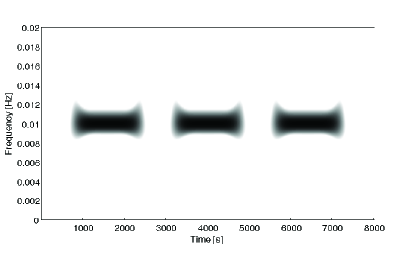
Figure 8: ASPWVD of an intermittent sinusoid of period 100 s, with $L_{g}=320$s and $L_{h}=320$s.

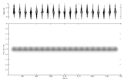
Figure 9: ASPWVD of an intermittent, amplitude modulated sinusoid of period 20 s, with $L_{g}=320$s and $L_{h}=320$s.

3.3 The Choi-Williams Distribution

Instead of using a separable smoothing kernel, several kernels have been developed that depend on the product of $\tau$ and $\nu$. One of the earliest examples is the Choi-Williams distribution (CWD) (Choi & Williams, 1989), which is characterized by the kernel

$$\Psi_{CWD}(\tau,\nu)=e^{-\frac{(2\pi\tau\nu)^{2}}{\sigma}}.$$ (13)

$\sigma$ is a positive parameter that jointly controls smoothing in time and frequency: a larger value for $\sigma$ gives less smoothing (Hlawatsch et al., 1995). In fact, as $\sigma\rightarrow+\infty$, the CWD tends to the WVD. Pure sinusoids have the ideal time-frequency resolution of the WVD, but all other signals are broadened when compared with the WVD (Hlawatsch & Urbanke, 1994).

Figure 10 shows the CWD of the synthetic DN lightcurve with $\sigma=100$. Reducing $\sigma$ to 0.1, as shown in figure 11, which increases the amount of smoothing, does not fully eliminate the ITs; further reductions in $\sigma$ have no noticeable affect. In fact, ITs due to different frequency components occurring at the same time cannot be attenuated completely if we use the CWD (Hlawatsch et al., 1995). In Kiss & Szatmáry (2002), the good time resolution of the CWD enables the increase in frequency of the main pulsation to be seen clearly, and the strong interference terms caused by the interaction of the main component with its harmonics are not a problem, since they can be easily identified as spurious using the periodogram. However, for our data, since complete IT attenuation is required, the CWD is not ideal.

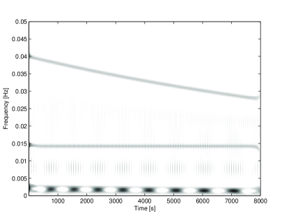
Figure 10: CWD of the synthetic DN lightcurve with $\sigma=100$.

Figure 11: CWD of the synthetic DN lightcurve with $\sigma=0.1$.

3.4 The Born-Jordan Distribution and Cone-shaped Kernel Representation

If we require a TFR that preserves finite time- and frequency-support, then the simplest choice for $\Psi(\tau,\nu)$ is

$$\Psi_{BJ}(\tau,\nu)=\frac{\sin(\pi\tau\nu)}{\pi\tau\nu},$$ (14)

which defines the Born-Jordan distribution (BJD). This kernel does not admit smoothing of ITs in the frequency direction. Allowing smoothing of the BJD in frequency gives the Zhao-Atlas-Marks representation (Zhao et al., 1990), also known as the cone-shaped kernel representation (CKR), with the kernel

$$\Psi_{CKR}(\tau,\nu)=g(\tau)|\tau|\frac{\sin(\pi\tau\nu)}{\pi\tau\nu}$$ (15)

where $g(\tau)$ is any window function (Hlawatsch et al., 1995). The length of the window, $L_{g}$, again controls the amount of frequency smoothing.

Figure 12 shows the CKR of the synthetic DN signal with $L_{g}=$ 1000 s, which is the minimal length required to completely attenuate the ITs between the QPOs. The frequency resolution is comparable to the SPWVD and ASPWVD, and the edge effects are less marked than those of the ASPWVD. Notice, however, that the way in which the CKR smooths the signal in figure 12 causes the QPOs to appear to oscillate slightly in frequency. IT attenuation in the CKR is complex. For components which are close in frequency, the attenuation will depend on the time distance, $\tau$, between the components. If the time distance between two components is $\tau$, and $0<|\tau|<\frac{1}{2}L_{g}$ then the resulting IT will be amplified, rather than attenuated. However all terms (signal and IT) with $|\tau|>\frac{1}{2}L_{g}$ will be completely suppressed. We are thus faced with a dilemma: increasing $L_{g}$ improves frequency resolution, but also makes it more likely that ITs will fall in the $0<|\tau|<\frac{1}{2}L_{g}$ range, and hence be enhanced (Hlawatsch et al., 1995).

The CKR of the intermittent 100 s is shown in figure 13. In comparison with the previous two TFRs, the frequency resolution of the CKR is excellent. The time resolution is similar to that of the ASPWVD. ITs, although of low amplitude, are present, again appearing as a low amplitude 100 s oscillation between the true signal bursts.

Figure 14 shows the CKR of the intermittent, amplitude-modulated 20 s oscillation signal. The amount of smoothing in time required to remove the low-frequency ITs in the synthetic DN lightcurve results in the signal terms of the intermittent DNO being completely smoothed. In addition, the ITs are amplified (due to the complicated IT attenuation of the CKR kernel) and smoothed , resulting in the appearance of five continuous frequency bands, even more pronounced than those in the ASPWVD of the same signal. While this is a somewhat extreme example, it does show that the effects of the CKR must be carefully monitored.

As the CKR can attenuate signals in a manner that is not easy to predict, and can amplify ITs rather than attenuating them, it is not ideal for analyses requiring significance testing. For large amplitude signals where this is not the case, the CKR can be an extremely useful tool: in figures 2 to 4 of Buchler, Kolláth & Cadmus (2004), for example, the CKR is seen to give sharp images for the five large-amplitude irregular pulsators under discussion. The fundamental period and harmonics are visible; and since these are relatively widely spaced in frequency, the ITs are easily identifiable.

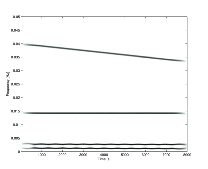
Figure 12: CKR of the synthetic DN lightcurve with $L_{g}=1000$s.

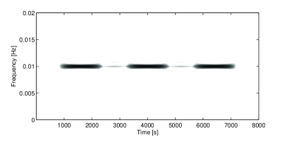
Figure 13: CKR of a intermittent sinusoid of period 100 s, L_g=1000s.

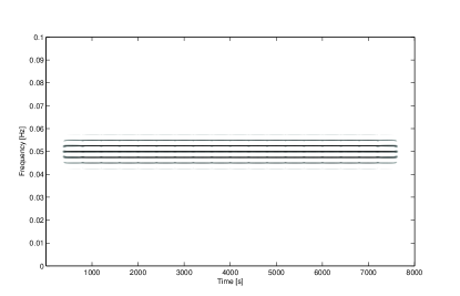
Figure 14: CKR of an intermittent, amplitude modulated sinusoid of period 20 s, with $L_{g}=1000$s and $L_{h}=1000$s.

3.5 Gabor Spectrogram

The (Gabor) spectrogram’s kernel is given by

$$\Psi_{SPEC}=W_{h}(-\tau,-\nu),$$ (16)

where $W_{h}(-\tau,-\nu)$ is the WVD of $h(t)$, any short-time analysis window localised around $t=0$ and $f=0$. This means that the time-frequency resolution of the spectrogram is dictated by the resolution of $h(t)$, rather than that of the analysed signal. Smoothing in the spectrogram is thus extensive, resulting in virtually complete interference attenuation, but also in poor time-frequency resolution (Hlawatsch & Boudreaux-Bartels, 1992). The choice of $h(t)$ determines the trade-off between the time spread and the frequency spread of the smoothing function: time resolution is proportional to the time duration of $h(t)$, while frequency resolution is proportional to the bandwidth of $h(t)$.

Figure 15 shows the Gabor spectrogram of our synthetic DN signal, using a Gaussian window of length 2000 s, which is the shortest that allows resolution of the QPO components. Each component is clearly visible, and there are no interference terms, although some smoothing is apparent near the ends.

Figure 16 shows the Gabor spectrogram of an intermittent sinusoid, using the same window as in the previous example. We see that requiring good frequency resolution has again resulted in poor time resolution. Indeed, as Cohen (1989) and Zhao et al. (1990) point out, if one wishes to have accurate time and frequency measurements using the spectrogram, two separate analyses must be undertaken, using windows of different length.

Boyd et al. (1995) use the Gabor transform to investigate HD 60435 (see fig. 7 of Boyd et al. (1995)). Because they are analysing a specific oscillation (11.64 min) they are able to choose an analysis window width which gives the required time-frequency resolution in this narrow frequency band. Belloni, Parolin & Casella (2004) also consider a relatively narrow frequency band, and are hence able to achieve an appropriate time-frequency resolution balance. Dolan et al. (1998) gives one of the the few examples of the analysis of a transient signal with the Gabor spectrogram, but since the frequency range is relatively narrow, they are able to choose a window length which gives the optimal time-frequency resolution for analyzing the signal.

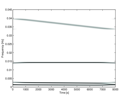
Figure 15: Gabor spectrogram of the synthetic DN lightcurve, with $L_{g}=2000$s.

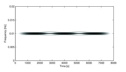
Figure 16: Gabor spectrogram of an intermittent sinusoid, with window length 2000s.

3.6 The Wavelet Scalogram

The wavelet scalogram is the affine counterpart of the Gabor spectrogram. Just as the Gabor spectrogram can be calculated using any short-time analysis window that is localised around $t=0$ and $f=0$, the wavelet scalogram can be calculated using any “mother wavelet” $\psi_{0}$ that is centered in the neighbourhood of $t=0$, has zero average ($\int^{\infty}_{\infty}\psi_{0}(t)dt=0$) and is normalized to have unit energy ($\int^{\infty}_{\infty}|\psi_{0}(\omega)|^{2}d\omega=1$) (Mallat, 1998). From the mother wavelet, $\psi_{0}$, we define a family of functions

$$\psi_{t,a}(s)=\frac{1}{\sqrt{a}}\psi_{0}\left(\frac{s-t}{a}\right).\hskip 28.45274pts>0,b\in\mathbb{R}$$ (17)

Then for a given $\psi_{t,a}$, the wavelet scalogram, $A_{SCALO}$, has the affine kernel

$$\Psi_{SCALO}(\tau,\nu)=W_{\psi_{t,a}}(\tau,\nu)$$ (18)

where $W_{\psi_{t,a}}(\tau,\nu)$ is the WVD of $\psi_{t,a}$.

The choice of mother wavelet depends on the signal to be analysed and the type of analysis desired. If the shape of the signal to be detected is known, then the wavelet with the nearest matching shape should be chosen (Meyers, Kelly & O’Brien, 1993). Considering the often (amplitude modulated) sinusoidal shape of DNOs and QPOs, smoothly oscillating wavelets such as the Morlet, Mexican Hat and Paul wavelet are indicated, rather than the abrupt step function of the Haar wavelet, or the spiky Daubechies wavelet.

An additional consideration is that in the scalogram of a complex wavelet, such as the Morlet, phase information from the data is lost. A scalogram using a complex wavelet has constant power across the time duration of an oscillation, and the time locations of maxima and minima in the oscillation cannot be detected. For real wavelets, however, such as the Mexican Hat wavelet, phase and amplitude information is superposed in the time-frequency plane and extrema are easily detected (Percival & Walden, 2000) - a feature that is not present in any of the TFRs studied so far in this paper.

In order to explore fully the behaviour of the wavelet scalogram we thus investigate two smooth wavelets with very different analytical capabilities: the complex Morlet wavelet and the real Mexican Hat wavelet.

3.6.1 The Morlet Wavelet

The Morlet wavelet is described by

$$\psi(\eta)=\pi^{-\frac{1}{4}}e^{-\frac{1}{2}\eta^{2}}e^{(i\omega_{0}\eta)}$$ (19)

where $\eta=t/s$ is a non-dimensional time parameter and $\omega_{0}$ is the wavenumber (Torrence & Compo, 1998). The Morlet wavelet is essentially a complex exponential of frequency $\frac{\omega_{0}}{2\pi}$, modulated in amplitude by a Gaussian window (Percival & Walden, 2000). We have chosen to use $\omega_{0}=6$ in our analysis, which gives a Morlet wavelet which has 5 oscillations. This is the most commonly used value of $\omega_{0}$, but is also appropriate given the QPO detection criteria which will be discussed in section 4.

Since the wavelet is localized in time and scale, the wavelet scalogram at a particular time $t^{\prime}$ is affected only by signal values close to $t^{\prime}$, in a radius that depends on the width of the wavelet as determined by the scale $a$. The cone of influence (COI) of a point $(t^{\prime},s)$ on the time-scale plane is the set of all points $(t^{\prime\prime},s)$ for which $x(t^{\prime})$ affects $A_{SCALO}(t,a)$. Finite data length means that for points near the beginning or end of the data set, the support of $A_{SCALO}(t,a)$ effectively includes a number of points with zero amplitude (i.e. points before or after measurement started), and therefore has significantly reduced power. Torrence & Compo (1998) define the $e$-folding time $\tau_{s}$ for the wavelet as the time-radius at which the wavelet power first drops by a factor of $e^{-2}$ at an edge. The time extent to which these ‘edge effects’ affect the wavelet scalogram depends on the scale of the wavelet and the type of wavelet; at shorter scales (shorter periods) the effect is minimal, while at very long scales, the effect is marked. For the Morlet wavelet, $\tau_{s}=\sqrt{2}s$ (Torrence & Compo, 1998).

It is preferable to plot the wavelet scalogram as a function of frequency rather than scale. For the Morlet wavelet, the equivalent Fourier period for a given scale $s$ is

$$\textrm{Period}\ =\frac{4\pi s}{\omega_{0}+\sqrt{2+{\omega_{0}}^{2}}}$$ (20)

(Meyers, Kelly & O’Brien, 1993; Torrence & Compo, 1998). Figure 17 shows the Morlet scalogram of the synthetic DN lightcurve. While all components are clearly visible, and there are no interference terms, the lpDNO and especially the DNO are not well resolved in frequency. The large black ‘U’ marks the e-folding time at each scale: points outside this region are distorted by edge effects. It is clear that while edge effects are minimal at high frequencies, they become significant at low frequencies.

In both the Morlet scalogram of the intermittent sinusoid with period 100 s (figure 18) and the intermittent, amplitude-modulated sinusoid with period 20 s (figure 19), we have an IT-free TFR in which the signal is well resolved in time, but this has come at the expense of poor frequency resolution: the Morlet scalogram has by far the worst frequency resolution of any of the TFRs investigated so far. There is, however, a way we can compensate for this poor frequency resolution, while maintaining the excellent time resolution and IT-free properties of this TFR.

Delprat et al. (1992) show that for complex wavelets such as the Morlet, the wavelet scalogram of a monocomponent signal with slowly changing low frequency reaches a maximum at the instantaneous frequency $\phi^{\prime}(t)$ of the signal. Mallat (1998) extends this proof to include the accurate measurement of the instantaneous frequency of multiple components changing rapidly at high frequency. Thus the points $(\bar{t},\bar{f})$ at which the Morlet scalogram $A_{MORLET}(t,f)$ has a local maximum in frequency, i.e. for which

$$\begin{array}[]{ccc}\frac{\partial A_{MORLET}(t,f)}{\partial f}=0&\textrm{and}&\frac{\partial^{2}A_{MORLET}(t,f)}{\partial f^{2}}<0,\\ \end{array}$$ (21)

can be used to plot the instantaneous frequency of our signal accurately in the form of wavelet ridges(Mallat, 1998).

Figures 20, 21 and 22 again show the Morlet scalograms of our three test signals, but with the inclusion of wavelet ridges. Figure 17 looks pleasingly close to the ideal TFR shown in figure 1. Both figures 21 and 22 show wavelet ridges at frequencies other than the instantaneous frequency of the signal, but as these occur only at very low amplitudes they do not present the interpretational challenge that interference terms did in previous TFRs.

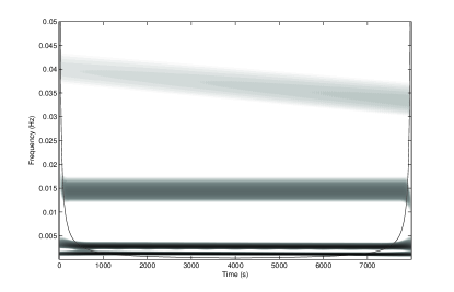
Figure 17: Morlet scalogram of the synthetic DN lightcurve.

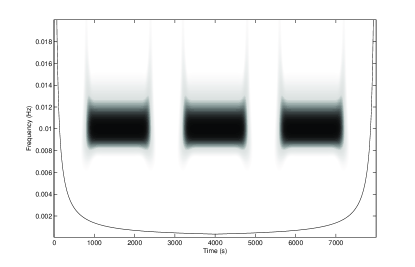
Figure 18: Morlet scalogram of the 100 s intermittent sinusoid.

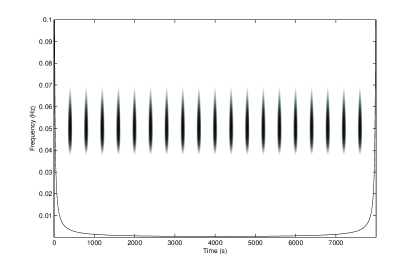
Figure 19: Morlet scalogram of the 20 s intermittent, amplitude modulated sinusoid.

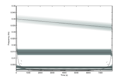
Figure 20: Morlet scalogram of the synthetic DN lightcurve, with ridges.

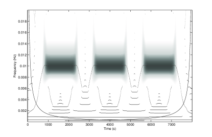
Figure 21: Morlet scalogram of the 100 s intermittent sinusoid, with ridges.

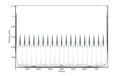
Figure 22: Morlet scalogram of the 20 s intermittent, amplitude modulated sinusoid, with ridges.

3.6.2 The Mexican Hat Wavelet

One of the most commonly used real wavelets is the Mexican Hat Wavelet (MHAT), given by the normalized second derivative of a Gaussian function:

$$\psi(\eta)=\frac{1}{\sqrt{\Gamma(2.5)}}(1-\frac{1}{\eta^{2}})e^{\frac{-\eta^{2}}{2}}$$ (22)

where again $\eta=t/s$. The equivalent Fourier period for a given scale $s$ is

$$\textrm{Period}\ =\frac{2\pi s}{\sqrt{2.5}}.$$ (23)

which effectively increases the minimum observed time-scale from $2dt$ to $7.95dt$ (McAteer et al., 2007). As a result, the MHAT wavelet is not useful for examining very short period phenomena. Figure 23 shows the MHAT scalogram of the synthetic DN signal. Notice that the highest frequency achievable is 0.03 Hz, which is below the starting frequency of the DNO. It is clear that the frequency resolution of the MHAT wavelet is considerably worse even than that of the Morlet wavelet. The usefulness of the MHAT wavelet is, however, apparent in the appearance of the lpDNO and the QPOs in the scalogram: individual extrema are discernable (the wavelet scalogram is an entirely positive TFR, so all signal extrema appear as maxima in the wavelet scalogram (Mallat, 1998)).

Similar to the wavelet ridges of the Morlet wavelet, the points $(\bar{t},\bar{f})$ at which the MHAT scalogram $A_{MHAT}(t,f)$ has a local maximum in time, i.e. for which

$$\begin{array}[]{ccc}\frac{\partial A_{MHAT}(t,f)}{\partial t}=0&\textrm{and}&\frac{\partial^{2}A_{MHAT}(t,f)}{\partial t^{2}}<0,\\ \end{array}$$ (24)

form maxima lines which identify maxima across frequencies (Mallat, 1998). Maxima lines are traditionally used to detect singularities and discontinuities. Polygiannakis et al. (2003) and McAteer et al. (2007), for example, use maxima lines to investigate the sunspot index and solar flare x-ray emission respectively. For our data, however, maximal lines can be used to detect the extrema in quasi-periodicities, which can be used to measure coherence, investigate phase relationships between different frequency phenomena and construct O-C diagrams. Figures 24 and 25 show the MHAT scalogram of the synthetic DN light curve and the 100 s intermittent sinusoid respectively, with the addition of maxima lines.

Both the Morlet scalogram with the addition of wavelet ridges and the MHAT scalogram with the addition of maxima lines provide valuable information in the analysis of our data. To facilitate easy analysis, we combine the information provided by the wavelet ridges and maxima lines on a single ‘Morlet ridged scalogram’: we plot all wavelet ridges, but only those points of the maxima lines which intersect with wavelet ridges. Figure 26 shows the our final TFR of the synthetic DN signal. Here we finally have a TFR in which all frequency components can be seen clearly, as well as the times at which each component has an extremum.

At least in the case of noise-free signals, it is clear that the Morlet ridged scalogram is the TFR best suited to our needs, providing excellent frequency resolution over a broad frequency ranges, combined with the time resolution needed to resolve intermittent signals. However, when analysing real data the statistical properties of the TFR are important for judging the likelihood that a detected oscillation is a true signal, and not an artefact of the noise. It thus behoves us to investigate the statistical properties of each of our six kernels, before declaring a winner.

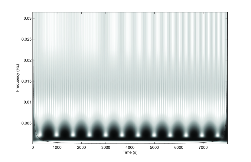
Figure 23: MHAT scalogram of the synthetic DN lightcurve.

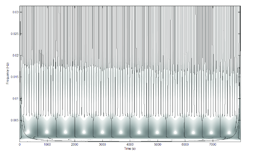
Figure 24: MHAT scalogram of the synthetic DN lightcurve with ridges.

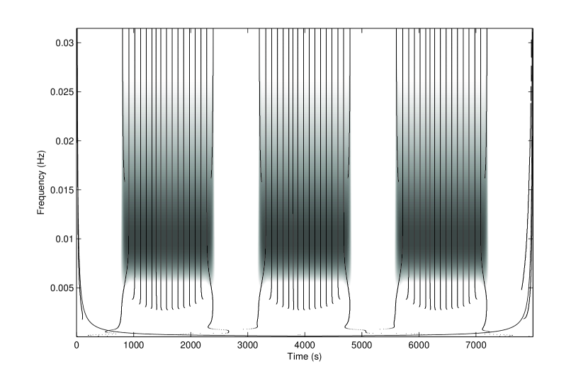
Figure 25: MHAT scalogram of the 100s intermittent sinusoid with ridges.

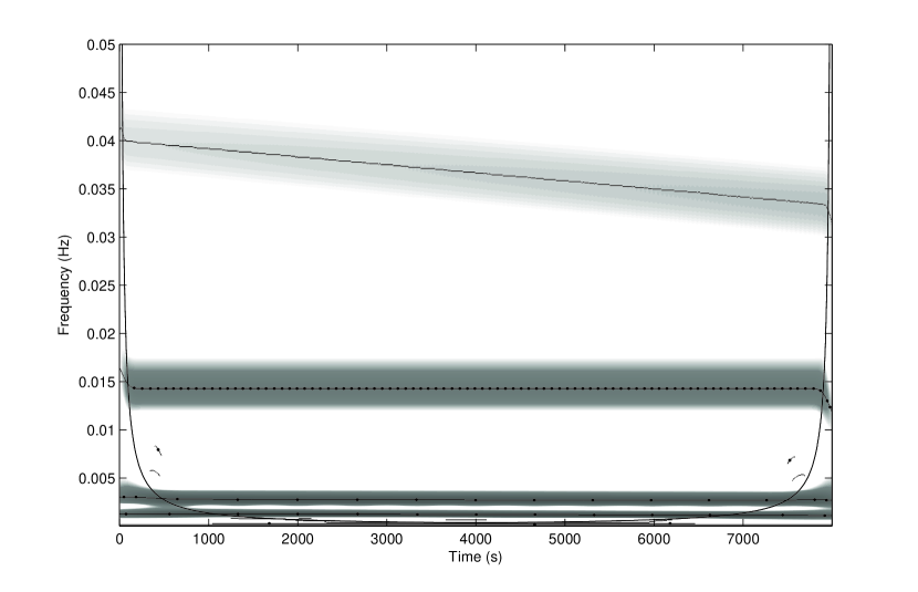
Figure 26: Morlet ridged scalogram of the synthetic DN lightcurve with wavelet ridges and maxima points.

3.7 Statistical Properties of TFRs

We assume that we have a non-stationary deterministic signal superimposed on weakly stationary non-white noise. This is not an unreasonable assumption: the noise spectrum of our data changes very slowly if at all over the duration of an observing run. We will discuss methods of estimating the power spectrum of the noise in section 4.2, but note here that the assumption of weak stationarity ensures that the periodogram can be used as an estimator for the power spectrum of the noise (Timmer & Koenig, 1995).

The WVD of a realization of a stochastic signal is an estimator for the theoretical WVD of the generating process (Mecklenbräuker & Hlawatsch, 1997). For a weakly stationary noise process with power spectrum $S(f)$, the expected value of the WVD, $E[W_{x}(t,f)]$, is given by the power spectrum of the process:

$$E[W_{x}(t,f)]=S(f)$$ (25)

(Qiu, 1993). For a deterministic signal corrupted with independent, identically distributed (i.i.d) gaussian noise with power spectrum $S_{noise}(f)$, the expected value of the WVD is the sum of the WVD of the signal and the spectrum of the noise:

$$E[W_{x}(t,f)]=W_{signal}+S_{noise}(f)$$ (26)

(Flandrin & Martin, 1984). The WVD is thus a biased estimator of the signal, and the larger $S_{noise}(f)$, the worse the bias. The WVD of the noisy signal, since it is determined by the power spectrum of the noise, is also not consistent: $W_{x}(t,f)\sim S_{noise}(f)\frac{\chi_{2}^{2}}{2}$.

Thus the WVD suffers from the same estimation problems as the periodogram. However, by estimating the power spectrum of the noise, confidence contours (the 2-D equivalent of confidence levels) can be used to determine regions in the time-frequency plane at which the signal has power significantly above that expected for pure noise (see Torrence & Compo (1998) for a detailed discussion of confidence contours for the wavelet scalogram).

The expected values of any Cohen TFR of a deterministic signal corrupted with i.i.d gaussian noise are also given by the sum of the noise-free TFR and the power spectrum of the noise, as was the case for the WVD. Thus these TFR estimators, which include the CWD, the BJD and the Gabor spectrogram, are also biased, with the amount of the bias depending on the noise level. We also have $C_{x}(t,f)\sim S_{noise}(f)\frac{\chi_{2}^{2}}{2}$ (Posch, 1990). In general, the variance of the TFR will depend on the amount of smoothing by the kernel: more smoothing results in a lower variance (Williams, 1998). The BJD is the minimum variance distribution for white noise (Hearon & Amin, 1995), while Williams (1998) shows that the Gabor spectrogram, when a rectangular window is used, gives the best performance of all Cohen TFRs in the presence of non-white noise, as it has the smallest variance.

For the SPWVD with $L_{g}=M$, for a deterministic signal corrupted by i.i.d gaussian noise, $C_{SPWVD}(t,f)\sim\frac{2}{2M-1}S_{noise}(f)\frac{\chi_{2}^{2}}{2}$ (Flandrin & Martin, 1984). Thus the variance of the SPWVD decreases as the length of the time-smoothing window increases.

For the ASPWVD, with $L_{g}$ at scale $s$ given by $M_{s}$, then for a deterministic signal corrupted by i.i.d gaussian noise,

$$A_{ASPWVD}(t,s)\sim\frac{2}{2M_{s}-1}S_{noise}(s)\frac{\chi_{2}^{2}}{2}$$ (27)

(Flandrin & Martin, 1984). Thus the variance of the ASPWVD decreases as the window length increases, as in the case of the SPWVD, but also depends on the analysing scale $s$.

Since the CKR’s integrals with respect to frequency, and over the entire time-frequency plane, are zero (because $\Psi_{CKR}(\tau,\nu)$ is zero on the entire $\nu$-axis), the CKR is not an energy distribution in the statistical sense (which is why we refer to it as a representation, rather than a distribution) (Hlawatsch et al., 1995). This means that its expected value is not related to the power spectrum as for the other TFRs. The CKR of a deterministic signal corrupted by i.i.d gaussian noise is the sum of the CKR of the noise-free signal and $D(t,f;g)$, where

$$D(t,f;g)=\int_{-\infty}^{\infty}g(\tau)|\tau|r(\tau)e^{-i2\pi f\tau}d\tau$$ (28)

and $r(\tau)$ is the auto-covariance of the noise. This means that for white noise, $D(t,f;g)=0$, and the CKR is an unbiased estimator (Oh & Marks, 1992). However, Hearon & Amin (1995) show that of all the Cohen TFRs the CKR has the highest variance, and hence the least desirable performance in the presence of noise. In addition, confidence contours cannot easily be constructed for the CKR since the stochastic distribution of the CKR is not calculable from the power spectrum as is the case for the other TFRs.

Percival (1995) shows that the time integral of the wavelet scalogram can be used as an unbiased, consistent estimator for the power spectrum. It is also the minimum affine variance estimator, and we have $A_{SCALO}\sim\frac{1}{2}S_{noise}\chi_{2}^{2}$. Thus from a statistical point of view, the wavelet scalogram is also the best TFR to use for our data.

4 Application of Time-Frequency Techniques to VW Hyi

In this section we use the Morlet ridged scalogram introduced in the previous section to analyse quiescent and outburst lightcurves from VW Hyi. Our purpose is threefold. Firstly, since all of these runs have been analysed in detail previously, we see how previously detected DNOs and QPOs appear in the wavelet scalogram, and hence build up a set of criteria for objectively detecting QPOs using the wavelet scalogram. We then use these criteria to see if there are QPOs in the VW Hyi data which have not been identified by the old methods. Finally, we use the wavelet methods to investigate the non-stationary behaviour of all DNOs and QPOs detected.

This analysis establishes the reliability of the Morlet ridged scalogram (we find that all previously identified DNOs and QPOs are detected by the scalogram), and provides an opportunity to compare the information elicited by the new techniques with that given by traditional techniques such as the Fourier Transform and O-C curves.

4.1 Observations

VW Hydri is an SU UMa dwarf nova with an outburst time scale of the order of 28 days (Warner, 1995). Since it is circumpolar at the Sutherland site of the South African Astronomical Observatory, and is relatively bright (9-13 mag), VW Hyi presents an extended season for maximum time-resolution observation. In addition to quiescent observations, many observations have been made selectively towards the end of outburst as the star returns to quiescence specifically to study DNO and QPO behaviour (Warner & Woudt, 2006), and several groups of runs taken on consecutive nights allow for the study of persistent or evolutionary phenomena across nights.

Our VW Hyi data are from the UCT archive, and have been previously analysed in Woudt & Warner (2002a), Woudt & Warner (2002b), Warner, Woudt & Pretorius (2003), Warner & Woudt (2006) Pretorius, Warner & Woudt (2006) and Warner & Pretorius (2008). Details of the individual observing runs for outburst and quiescent observations are given in tables 2 and 3 respectively. All observations were taken at the Sutherland site of the South African Astronomical Observatory, using the 20”, 40” or 74” telescope as indicated. Data acquisition for observations on the 20” and 40” telescope up to and including run s5248 used the UCT photometer (Nather & Warner, 1971); subsequent runs on this telescope and the 74” were made using the University of Cape Town CCD (O’Donoghue, 1995) operating in frame-transfer mode. Most CCD observations were taken in white light; observations made with a B filter are marked with an asterisk.

The data were pre-whitened by removing the mean and first-order trend. VW Hyi lightcurves also frequently show a strong orbital hump, which can dominate the periodogram and wavelet scalogram. To avoid this, and enable smaller amplitude periodicities to be examined, we removed a sinusoid and first harmonic at the orbital hump frequency.

4.2 Power Spectrum Estimation

Torrence & Compo (1998)’s statistical detection of significant oscillations in the wavelet scalogram requires estimation of the periodogram of the noise spectrum of the signal, a perennial problem in noisy astronomical time series analysis. Vaughan (2005) suggests fitting a linear function to the log-periodogram, since his data show a red-noise power spectrum well modeled by power law (i.e. linear in log-space). Flickering also gives our data a red noise spectrum, but CV flickering has less power at very low frequencies than the X-ray data of Vaughan (2005); we therefore fit a low-order polynomial (generally between third and fifth-order) in log-space, using an OLS fitting programme.

To check that our assumption of a stationary noise structure for each data set was correct, we calculated the best-fit noise-model for sections of each run as well as for the entire run; in all cases we found that the models for each section were very similar to the model for the complete time series.

4.3 Analysis

VW Hyi outbursts can be divided into four groups: superoutburst, long normal outburst, medium normal outbursts and short normal outbursts (Woudt & Warner, 2002a). The RASNZ VW Hyi data, spanning 1972-2004, have been used to construct average outburst profiles (figure 27), onto which each outburst observation can be placed (Woudt & Warner, 2002a). Each observation is thus assigned a phase (column ‘Start’ in tables 2 and 3), relative to the arbitrary $T=$0 d (column ‘T=0’ in tables 2 and 3) of the template. We have assigned quiescent observations a phase relative to $T=$0 d of the next outburst, as we have several quiescent observations occurring a few days before an outburst for which we also have data.

We computed the Morlet ridged scalogram for each run to see if previously detected QPOs were detected by the scalogram. We found that all previously detected QPOs were visible in the Morlet ridged scalogram, with power above the 95% confidence level and a single continuous instantaneous frequency line of stable or slowly changing frequency. We counted the number of extrema (given by the maximal points) which occurred during the time span of the confidence contour, and found that while 3 cycles (6 maximal points) were sometimes sufficient to have been identified as a QPO in the periodogram (e.g. run s0030), usually 5 or more cycles were present. We thus defined a QPO as at least 5 cycles (10 maximal points in the MHAT) at power above the 95% confidence level (on the Morlet spectrum), or 6 significant cycles spread over two confidence contours at similar frequency. We only deviated from this definition when there was a clear triplet of QPOs with fundamental, first and second harmonic, and one of these contained less than 5 cycles, in which case it was identified as a QPO (e.g. run s1307). We used the instantaneous frequency to find the (average) period of the detected QPO.

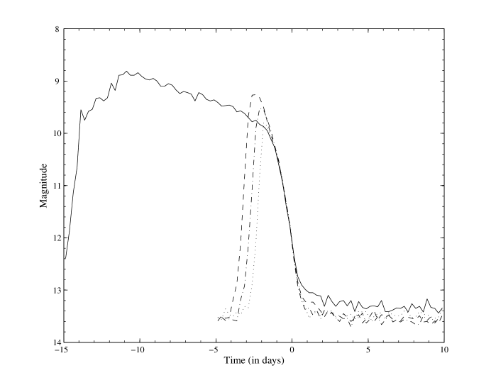
Figure 27: Averaged outburst profiles for the four different types of outburst seen in VW Hyi. Solid line indicates superoutburst, dashed line indicates long normal outburst, dash-dot indicates medium normal and dotted indicates short normal outburst.

Table 2: VW Hyi: Outburst observations from the UCT archive. Runs marked with an asterisk were taken using a B filter.

Run	Telescope	Length	Int	Outburst	HJD Start	$T=0$	$T$ Start
		(hrs)	time (s)	Type	$+2440000$	(d)	(d)
s0018	20	2.04	2	L	1572.52	1572.75	-0.23
s0019	20	4.30	5	L	1573.44	1572.75	0.69
s0026	20	3.32	5	L	1574.50	1572.75	1.75
s0030	20	6.92	5	L	1575.47	1572.75	2.72
s0110	40	2.47	2	Super	1662.30	1677.20	-14.90
s0111	40	0.97	2	Super	1662.41	1677.20	-14.79
s0112	40	2.31	2	Super	1662.48	1677.20	-14.72
s0122	40	2.56	5	Super	1675.33	1677.20	-1.87
s0124	40	1.84	5	Super	1676.37	1677.20	-0.83
s0127	40	3.77	4	Super	1677.29	1677.20	0.09
s0129	40	1.86	5	S	1691.30	1690.20	1.10
s0480	40	1.73	5	Super	2017.38	2022.65	-5.27
s0484	40	3.91	4	Super	2023.31	2022.65	0.66
s1277	40	1.78	4	M	2352.39	2354.20	-1.81
s1307	40	1.33	4	M	2354.39	2354.20	0.19
s1322	40	4.91	4	M	2355.39	2354.20	1.19
s1571	40	1.99	4	Super	2402.32	2403.40	-1.08
s1616	40	2.27	3	Super	2404.31	2403.40	0.91
s2241	40	2.63	5	Super	2758.41	2770.00	-11.59
s2243	40	1.65	5	Super	2759.40	2770.00	-10.60
s2623	40	3.60	5	M	3515.30	3514.60	0.70
s2911	40	3.14	4	L	4934.43	4937.10	-2.67
s2915	40	0.73	4	L	4937.28	4937.10	0.18
s2917	40	2.18	4	L	4939.49	4937.10	2.39
s3078	40	1.95	4	Super	5323.34	5328.50	-5.16
s3416	40	1.19	2	M	5967.55	5967.00	0.55
s5248	40	4.66	5	M	8202.36	8201.75	0.61
s6138_I	40	2.09	4	M	11898.28	11897.85	0.43
s6138_II	40	3.90	5	M	11898.43	11897.85	0.58
s6184	40	1.68	5	L	11957.28	11957.25	0.03
s6316	40	5.72	5	L	12354.24	12353.95	0.29
s6528_I	74	5.81	4	L	12520.22	12519.65	0.57
s6528_II	74	4.18	5	L	12520.47	12519.65	0.82
s7222_I*	74	3.61	4	Super	13007.31	13006.40	0.91
s7222_II*	74	3.03	4	Super	13007.46	13006.40	1.06
s7301	40	2.94	5	M	13087.24	13086.10	1.14
s7311*	74	5.41	4	M	13139.19	13138.95	0.24
s7342	40	3.07	5	M	13155.19	13154.90	0.29
s7621	40	4.03	6	L	13463.23	13463.10	0.13

Table 3: VW Hyi: Quiescent observations from the UCT archive

Run	Telescope	Length	Int	HJD Start	$T=0$	$T$ Start	HJD Next
		(hrs)	time (s)	$+2440000$	(d)	(d)	$+2440000$
s0073	40	2.83	5	1648.25	1613.00	-28.95	1677.20
s0077	40	4.11	5	1602.44	1580.00	-10.56	1613.00
s0085	40	1.67	5	1604.44	1580.00	-8.56	1613.00
s0093	40	3.33	5	1605.45	1580.00	-7.54	1613.00
s0102	40	1.31	5	1657.33	1613.00	-19.87	1677.20
s0105	40	1.80	2	1660.29	1613.00	-16.91	1677.20
s1414	40	2.89	4	2384.30	2370.00	-19.10	2403.40

We give a detailed discussion of several of the runs analysed, showing how DNOs and QPOs appear in real data and highlighting the additional information which the Morlet ridged scalogram makes available. Discussions of further runs are available in Blackman (2008).

4.3.1 s0110, s0122 and s0127

These three runs are part of a series of runs spanning a superoutburst. Run s0110 was taken on during the rise to supermaximum ($T=$14.90 d), while runs s0122 and s0127 were taken on consecutive nights during decline, from $T=-0.83$ to 0.09 d.

s0127 (figures 29 and 28) exhibits a plethora of phenomena, and is an excellent example of both the broad frequency range covered by DNOs and QPOs (from periods of 15 s to 1250 s) and the intermittent behaviour of these phenomena which have necessitated the development of the Morlet ridged scalogram. Figure 28 clearly shows the 27 s DNOs, increasing in period over the duration of the run to 34 s. There are also suggestions of the 15 s first harmonic for the first 3000 s, and again near the end of the run. Figure 29 shows the 450 s QPO found by Warner & Woudt (2006), as well as evidence of a 1250 s oscillation, changing to 1075 s after 8000 seconds, which we categorize as a subharmonic of the 480 s oscillation.

Runs s0110 and s0122 are included to contrast the Morlet ridged scalograms of data with and without significant oscillations. Run s0110 (figure 30) shows no oscillations. Although there are regions of significant power, the instantaneous frequency fluctuates hugely, and hence these regions are not identified as indicating the presence of QPOs. In contrast, in s0122 (figure 31) we see in addition to the 410 s QPO identified in Woudt & Warner (2002a) a 909 s oscillation persisting throughout most of the run, especially prominent in the last half.

4.3.2 s0129

s0129 (figure 32) is a good example of the wavelet spectrum’s use in indicating oscillations of low coherence. In addition to the DNO (either DF or lpDNO) at 93 s identified by Woudt & Warner (2002a), there is evidence of power at about 33 s throughout the scalogram as well as three runs of QPOs with periods 578 s, 658 s and 714 s. The most coherent run lasts for only 5 cycles. Neither the 33 s nor the QPOs are visible in the power spectrum.

4.3.3 s1616

Run s1616 was taken at the end of return to quiescence after a superoutburst, at 0.912 d, and shows a typical triplet of QPO harmonics. A 694 s QPO appears twice in s1616, as well as a 1282 s QPO for the first half, and 7 cycles of 333 s QPO, giving the triplet of QPO fundamental, first and second harmonic. There is also evidence of an 87 s oscillation near the end of the run (not shown in figure 33); this may be either an lpDNO or the DNO fundamental.

4.3.4 s2241

Run s2241 (figure 34) was taken during superoutburst, and shows unclassified QPOs with a period of about 700 s, first detected by Woudt & Warner (2002a). The scalogram reveals the previously unrecognized fact that these QPOs are only present during the superhumps - in the top panel of figure 34 we show the raw lightcurve of s2241, showing the superhumps, which can be matched with the QPOs in the scalogram below. The scalogram enables us to see clearly where the oscillations begin and end, and for how many cycles they last. There is some evidence for a first harmonic at about 350 s, but this may be due to the non-sinusoidal profile of the QPOs.

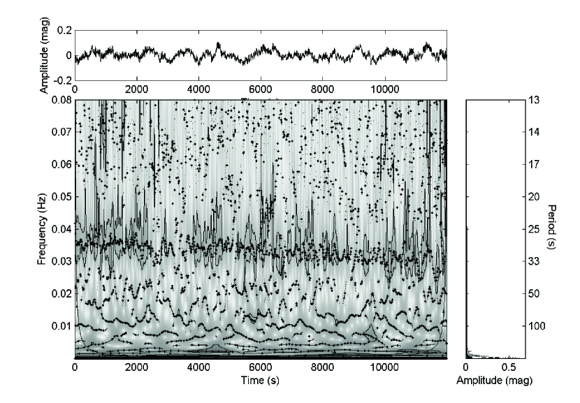
Figure 28: Prewhitened lightcurve, Morlet ridged scalogram and periodogram of run s0127.

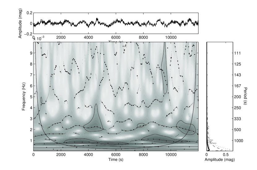
Figure 29: Prewhitened lightcurve, Morlet ridged scalogram and periodogram of run s0127 for the frequency range 0 - 0.01 Hz, showing QPOs.

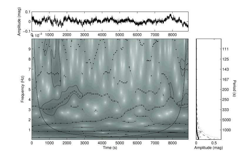
Figure 30: Prewhitened lightcurve, Morlet ridged scalogram and periodogram of run s0110. No oscillations are identified.

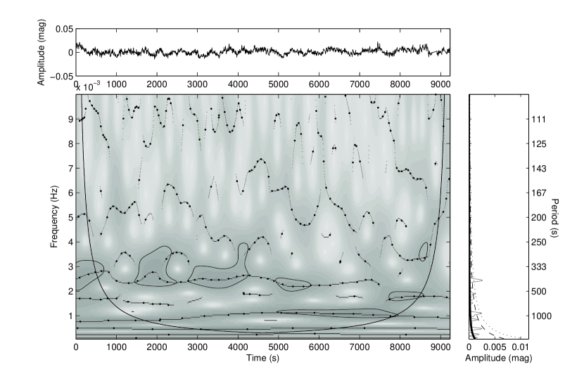
Figure 31: Prewhitened lightcurve, Morlet ridged scalogram and periodogram of run s0122, showing QPOs.

Figure 32: Prewhitened lightcurve, Morlet ridged scalogram and periodogram of run s0129.

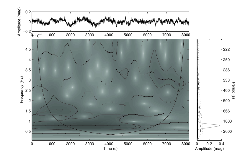
Figure 33: Prewhitened lightcurve, Morlet ridged scalogram and periodogram of run s1616.

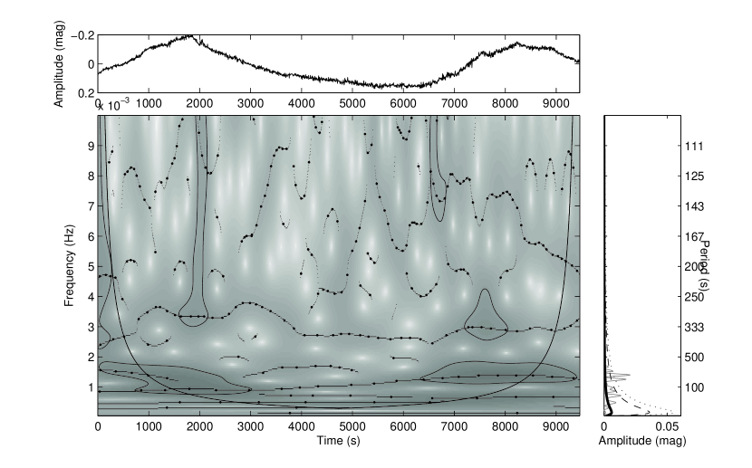
Figure 34: Raw lightcurve, Morlet ridged scalogram and periodogram of run s2241; note that the QPOs visible in the scalogram are only present during superhumps.

Table 4 summarizes the details of each oscillation detected in our analysis; we include the run number, the type of outburst, the start and end times of each oscillation (in seconds from the beginning of the run), the period of the oscillation at start and finish (in seconds), and the average amplitude (in magnitudes). Oscillations showing non-monotonic period changes were analysed in monotonic sections. For oscillations with periods $>$100 s the number of cycles observed is included. DNOs are classified as fundamental (DF), first(D1) or second harmonic(D2) or lpDNOs (DL). DNOs with periods between 70 and 120 s may be either fundamental period DNOs, or lpDNOs; we have decided to categorize all DNOs in this period range as lpDNOs. DNO-related QPOs are classified as fundamental (QF), first(Q1) or second harmonic (Q2) or subharmonic(QS). QPOs that do not appear to be DNO-related are classified as QU, and QPOs from quiescent light curves are classified as QQ. The second last column, ‘Prev?’, indicates whether the oscillation had been detected in previous analyses (‘y’) or not (‘n’), and the final column includes comments.

4.4 Results

We have identified some 62 new QPOs to add the existing 44, showing that the Morlet ridged scalogram is a useful, objective tool for the detection of quasi-periodicities. Figure 35 shows all the QPOs detected in our analysis (for ease of viewing, DNO-related QPO harmonics are shown at the implied fundamental). Previously studied QPOs (Woudt & Warner (2002a) or Warner & Woudt (2006)) are indicated by filled shapes; open shapes indicate QPOs that have been detected using wavelet analysis. Circles represent DNO-related QPOs, triangles those QPOs which have no DNO counterpart and squares indicate quiescent QPOs. Note that the large numbers of QPOs observed around $0<$T(d)$<1.15$ is at least partly due to the observing campaign of Brian Warner and Patrick Woudt, who selectively observed VW Hyi during late outburst.

All DNOs previously detected by Woudt & Warner (2002a) and Warner & Woudt (2006) were detected in the Morlet scalogram, as well as 2 new DNOs. This is unsurprising: DNOs in general have higher coherence than QPOs, and are hence more likely to be detected in periodogram analysis such as that used in Woudt & Warner (2002a) and Warner & Woudt (2006). Out of 24 outburst runs showing DNOs, including all those covered in Warner & Woudt (2006), we found DNO-related QPOs in each run. In addition, after finding a triplet of QPOs in s1616, close inspection of the FT and wavelet showed evidence of DNOs, although of very low coherence.

In previous work, DNOs with periods $\geq$ 70 s have been classified as DFs or lpDNOs almost arbitrarily; we have chosen to classify every DNO with period $\geq$ 70 s as a lpDNO. Using this classification, we find 8 previously observed lpDNOs, and we have discovered a further 7.

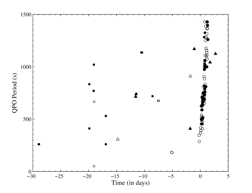
Figure 35: All QPOs analysed. Circles indicate DNO-related QPOs, triangles indicate unclassified outburst QPOs and squares indicate quiescent QPOs. Filled shapes are QPOs previously analysed in Warner I, II or IV; open shapes are QPOs added by this study.

Table 4: Table of QPOs detected in VW Hyi.

Name	Type	Osc	Osc end	Cycles	P start	P end	Mag	Class	Prev?	Comments
		start	end
s0018	L	650	1900	4	346	346	0.008	QF	n
s0018	L	1000	2000		75	75	0.007	DL	y
s0018	L	1500	2500		20	20	0.009	DF	y
s0018	L	3600	4600	3	286	286	0.007	QF	n
s0019	L	0	0		30	32	0.02	D1	y
s0019	L	1600	3200	3	487	487	0.05	Q1	y
s0019	L	3500	6250	7	370	400	0.04	Q1	n
s0019	L	5300	10000		20	20	0.02	D2	y
s0019	L	5300	10000	4	510	510	0.05	Q1	y
s0026	L	0	0	12	1042	1042	0.04	QU	y
s0030	L	10000	0	3	1124	1124	0.04	QU	y
s0111	Super	150	1300	4	307	307	0.007	QU	n
s0122	Super	0	5000	12	409	409	0.005	QU	y
s0122	Super	2000	8000	7	909	909	0.003	QU	n
s0127	Super	0	2400		27.9	28.7	0.02	DF	y
s0127	Super	1000	7000	5	1250	1250	0.03	QS	n
s0127	Super	2000	5000	7	454	454	0.02	QF	y
s0127	Super	3600	4800		29.3	29.3	0.02	DF	y
s0127	Super	5100	8200		29.7	30.5	0.03	DF	y
s0127	Super	6000	8200	5	498	498	0.02	QF	y
s0127	Super	8000	11000	3	1075	1075	0.03	QS	n
s0127	Super	9100	12000		32.2	32	0.015	DF	y
s0127	Super	10000	12000	4	487	487	0.037	QF	y
s0129	S	0	2500		33.5	33.5	0.02	D2	n
s0129	S	0	2500	4	578	578	0.02	Q1	n	Implied first harmonic
s0129	S	2000	3500		93	93	0.03	DL	y	DF in Warner - may be DL
s0129	S	3000	5000	3	658	658	0.02	Q1	n	Implied first harmonic
s0129	S	3500	5000		93	93	0.019	DL	y	DF in Warner - may be DL
s0129	S	5000	8000		33	33	0.02	D2	n
s0129	S	5000	8000	4	714	714	0.02	Q1	n	Implied first harmonic
s0484	Super	0	4000		30	32	0.02	D1	y
s0484	Super	0	3000	2.5	1282	1282	0.05	QF	y
s0484	Super	0	12000	5	2857	2757	0.05	QS	n
s0484	Super	2000	6000		68	68	0.009	DL	y
s0484	Super	4000	6500		37	37	0.02	D1	y
s0484	Super	4900	7500	6	488	488	0.03	Q1	y
s0484	Super	5000	14000	7	1325	1325	0.05	QF	y
s0484	Super	6500	12000		34	34	0.02	D1	y
s0484	Super	8000	14000	11	530	530	0.03	Q1	y
s1307	M	0	1000	2	500	500	0.01	QF	n
s1307	M	750	3000		31	31	0.005	DF	n
s1307	M	750	3000	5	250	250	0.005	Q1	n
s1307	M	1500	3000		18	18	0.005	D1	y
s1307	M	3500	4000		18	18	0.005	D1	y
s1307	M	3500	4500		38	38	0.005	DF	n
s1307	M	3500	4500	5	175	175	0.01	Q2	n
s1322	M	0	4000		31	31	0.01	D2	y
s1322	M	0	2500	11	357	357	0.05	Q2	n
s1322	M	3000	6000	4	476	476	0.05	Q2	y
s1322	M	6000	10000		29	30	0.01	D2	y
s1322	M	6000	10000	8.5	465	465	0.05	Q2	y
s1322	M	10000	12000		32	32	0.01	D2	y
s1322	M	12000	16000		28	31	0.01	D2	y
s1322	M	12500	15200	6	420	420	0.02	Q2	y
s1571	Super	0	0	5.5	1170	1170	0.005	QU	y
s1616	Super	0	2500	5	694	694	0.03	Q1	n	Implied fundamental
s1616	Super	0	5000	4	1282	1282	0.05	QF	n	Implied fundamental
s1616	Super	6000	8000		87	87	0.01	DL	n
s1616	Super	6000	8000	7	333	333	0.02	Q2	n	Implied fundamental - low coherence DNOs visible in periodogram
s2241	Super	0	2000	3	714	714	0.02	QU	y
s2241	Super	5500	9400	5	740	740	0.02	QU	y
s2243	Super	0	0		75	75	0.002	DL	y
s2623	M	0	2000		22	22	0.015	D2	y
s2623	M	0	2000	5	408	408	0.02	Q1	y
s2623	M	1000	2500	6	244	244	0.03	Q2	y
s2623	M	2000	4000		25	25	0.014	D2	y
s2623	M	4000	6000		24	24	0.014	D2	y
s2623	M	4000	9000	3	1000	833	0.005	QF	y	Implied fundamental
s2623	M	5000	7000	7	263	263	0.036	Q2	y
s2623	M	7000	10000	13	253	253	0.035	Q2	y
s2623	M	7000	10000	6	500	500	0.02	Q1	n
s2623	M	7500	10000		26	27	0.021	D2	y
s2623	M	10000	12500		25	27	0.019	D2	y
s2623	M	10000	12500	4	416	416	0.007	Q1	n
s2915	L	700	1500	4	250	250	0.006	Q1	n
s2915	L	1500	2500		20	20	0.011	D1	y
s2915	L	1800	2300	2	250	250	0.006	Q1	n
s3078	Super	0	7000		14	14	0.004	DF	y
s3078	Super	400	6000		90	90	0.002	DL	n
s3078	Super	2000	4000	4	183	183	0.004	QF	n
s3078	Super	5500	6500	4	182	182	0.002	QF	n
s3416	M	0	1000		25	25	0.017	D1	y
s3416	M	0	1000	4	270	270	0.026	Q2	n
s3416	M	1200	2500		27	27	0.015	D1	y
s3416	M	1200	2600	4	350	350	0.06	Q1	y
s3416	M	2600	4200		27	27	0.017	D1	y
s5248	M	0	4000		36	36	0.02	D1	y
s5248	M	0	0		96	96	0.02	DL	n
s5248	M	500	4000	6	454	454	0.08	Q1	n
s5248	M	4000	8000		40	40	0.005	D1	y
s5248	M	4000	8000	5	694	694	0.07	QF	n
s5248	M	5500	13000	5	1030	1030	0.05	QF	y
s5248	M	5500	13000	3.5	2000	2000	0.06	QS	y
s5248	M	8000	16000		40	40	0.005	D1	y
s6138-I	M	0	3000		25	25	0.01	D1	y
s6138-I	M	0	2200		25	26	0.01	D1	y
s6138-I	M	0	2200	7	317	317	0.02	Q1	n
s6138-I	M	0	3000	3	1030	1030	0.03	QS	n
s6138-I	M	3200	5000	3	667	667	0.05	QF	n
s6138-I	M	3300	5000		26	28	0.01	D1	y
s6138-I	M	3300	5000	3	370	370	0.06	Q1	n
s6138-I	M	5000	7300		28	28	0.005	D1	y
s6138-II	M	0	3000		28	30	0.005	D1	y
s6138-II	M	0	5000		70	70	0.02	DL	y
s6138-II	M	5000	14000		30.6	30.6	0.007	D1	y
s6138-II	M	5000	14000	13	344	392	0.04	Q1	y
s6138-II	M	6000	14000	5	1450	1450	0.02	QS	n
s6138-II	M	7000	14000	11	769	769	0.04	QF	n
s6184	L	0	1000		24.8	27.8	0.02	DF	y
s6184	L	0	1800	5	370	370	0.01	QF	n
s6184	L	1000	2300		26	26	0.014	DF	y
s6184	L	1800	2300		83	83	0.01	DL	y
s6184	L	2300	3000		26	26	0.026	DF	y
s6184	L	2300	3800	3.5	418	418	0.024	QF	n
s6184	L	3000	3500		25	25	0.008	DF	y
s6184	L	3500	3800		26	26	0.014	DF	y
s6184	L	3800	5000		27	27	0.017	DF	y
s6184	L	3800	5000		74	74	0.016	DL	y
s6184	L	5000	5500		26	26	0.013	DF	y
s6184	L	5000	6000	2.5	390	390	0.01	QF	n
s6184	L	5500	6000		27	27	0.011	DF	y
s6316	L	0	2500		20	20	0.009	D1	y
s6316	L	0	2000	6	294	294	0.001	Q1	y
s6316	L	2500	4000		20	20	0.011	D1	y
s6316	L	4000	6000		20.5	20.5	0.006	D1	y
s6316	L	4000	6000		77	83	0.008	DL	n
s6316	L	4000	5000	5	227	227	0.015	Q1	y
s6316	L	6000	10000		21.8	21.8	0.01	D1	y
s6316	L	10000	18000		21	23	0.016	D1	y
s6316	L	10000	15000		87	87	0.012	DL	n
s6316	L	11000	18000	21	375	375	0.009	Q1	y
s6316	L	15000	18000		88	88	0.011	DL	n
s6528-I	L	0	6000		18	23	0.015	D2	y
s6528-I	L	0	6000	13	666	666	0.024	QF	n	Implied fundamental
s6528-I	L	6000	12000		21	21	0.01	D2	y
s6528-I	L	6000	12000	5	1299	1299	0.024	QS	n	Implied fundamental
s6528-I	L	12000	18000		23	23	0.011	D2	y
s6528-I	L	12000	18000	6	885	885	0.013	QF	n	Implied fundamental
s6528-I	L	18000	20800		23	23	0.009	D2	y
s6528-I	L	18000	20800		32	32	0.008	D1	y
s6528-I	L	18000	20800	2	1052	1052	0.017	QF	n	Implied fundamental
s6528-II	L	0	6000		24	24	0.007	D2	y
s6528-II	L	0	6000	21	370	370	0.015	Q2	n
s6528-II	L	6000	10000		24	24	0.008	D2	y
s6528-II	L	6000	10000		37	37	0.005	D1	y
s7222-I	Super	0	2000		27	27	0.01	D2	y
s7222-I	Super	0	10000	8	1282	1282	0.05	QF	n	Implied fundamental
s7222-I	Super	2000	4000		26	26	0.005	D2	y
s7222-I	Super	2000	4000	5	625	476	0.02	Q1	n
s7222-I	Super	3000	6000		27	29	0.011	D2	y
s7222-I	Super	6000	7500		31	31	0.011	D2	y
s7222-I	Super	6000	8000		38	38	0.013	D1	y
s7222-I	Super	6000	7500	6	270	270	0.01	Q2	y
s7222-I	Super	7000	9500	5	588	588	0.04	Q1	n
s7222-I	Super	7500	9500		29	29	0.015	D2	y
s7222-II	Super	0	2500		34	34	0.013	D2	y
s7222-II	Super	0	2500	3	549	549	0.045	Q1	n
s7222-II	Super	2500	4000		29	29	0.015	D2	y
s7222-II	Super	4500	8000	3	1136	1136	0.038	QF	n
s7222-II	Super	5000	9000	8	333	333	0.035	Q2	y
s7222-II	Super	5000	10000	5	555	555	0.037	Q1	n
s7222-II	Super	5500	7500		28	28	0.022	D2	y
s7222-II	Super	7500	8500		30	30	0.016	D2	y
s7222-II	Super	8500	9000		32	32	0.009	D2	y
s7222-II	Super	9500	1000		34	34	0.01	D2	y
s7301	M	0	2000		33	33	0.009	D2	y
s7301	M	2000	4000		32	30	0.015	D2	y
s7301	M	4000	6000		32	34	0.015	D2	y
s7301	M	4000	7000	8	454	454	0.036	Q2	n
s7301	M	6000	7000		29	29	0.014	D2	y
s7301	M	7000	9000		32	32	0.012	D2	y
s7301	M	7000	9000	5	456	456	0.05	Q2	n
s7301	M	9000	0		29	31.8	0.014	D2	y
s7311	M	0	0		90	90	0.014	DL	n
s7311	M	0	1000	3	312	312	0.014	Q1	y
s7311	M	1800	3500	8	294	294	0.017	Q1	y
s7311	M	2000	3500		19	19	0.008	D1	y
s7311	M	3500	6000		20	20	0.006	D1	y
s7311	M	6000	15000		14	14	0.015	D2	y
s7311	M	6000	7400		20	20	0.007	D1	y
s7311	M	6000	10000	12	316	316	0.008	Q1	y
s7311	M	7000	9000	4	476	476	0.028	QF	n	Implied fundamental
s7311	M	7400	10000		20	21	0.006	D1	y
s7311	M	10000	13000	9	333	333	0.028	Q1	y
s7311	M	10500	12500		21	21	0.01	D1	y
s7311	M	12500	0		21	22	0.009	D1	y
s7311	M	13000	16000	6	345	345	0.015	Q1	y
s7311	M	13000	16000	4	666	666	0.016	QF	y
s7342	M	0	0		20	20	0.006	D1	y
s7342	M	0	2000	7	236	236	0.009	Q2	y
s7342	M	1800	6000	5	714	714	0.006	QF	n
s7342	M	2000	6000	10	321	321	0.01	Q1	y
s7342	M	6000	0		14	14	0.015	D2	y
s7342	M	6000	8000		38	38	0.009	DF	y
s7342	M	6000	10000	14	136	136	0.005	Q2	n
s7342	M	8000	9200	5	256	256	0.015	Q1	y
s7342	M	8000	10000	4	500	500	0.009	QF	y
s7621	L	0	600		28	28	0.007	DF	y
s7621	L	600	2000		27	30	0.011	DF	y
s7621	L	4000	6000	5	454	454	0.012	QF	y
s7621	L	6000	11000	11	454	454	0.027	QF	n
s7621	L	8000	10000		31	33	0.008	DF	y
s7621	L	11000	14000		18	18	0.01	D1	y
s7621	L	11000	14000		38	38	0.013	DF	y

5 Discussion and Conclusion

Lightcurves that contain multiple non-stationary components cannot be satisfactorily analysed using the periodogram alone, as the periodogram obscures the time-varying nature of the signal. Time-frequency representations allow signals to be viewed in the time and frequency domains simultaneously, enabling non-stationary components to be analysed. Various TFRs have been used in astronomy, but only for signals that have very high signal-to-noise ratios, cover a narrow frequency band, and have only a few components. For signals such as those found in cataclysmic variable stars, which contain multiple quasi-periodicities over a broad frequency range, against high background noise, it is not clear which of the TFRs used in the literature (if any) is most appropriate.

We have investigated the time-frequency resolution of six TFRs, using three synthetic signals mimicking the key features of our data: broad frequency range, multiple components (some close together in frequency), amplitude modulation and intermittency. Interference terms are produced in many TFRs, so for our data we had to tune the TFRs to completely attenuate ITs, which could otherwise be mistakenly identified as signal terms. We found that the CWD could not be tuned to completely remove ITs for signals with components that overlap in time, and hence was not appropriate for our data. The Gabor spectrogram cannot provide simultaneously high time and frequency resolution over the wide frequency range of our data. While both the CKR and the ASPWVD gave good time and frequency resolution over a range of frequencies, they could not completely attenuate ITs at very high frequencies; the only TFR with achieved this was the wavelet scalogram. However, at high frequencies the wavelet scalogram, when tuned for high time resolution, did not have good frequency resolution. By computing the wavelet ridges of the Morlet scalogram, however, this shortcoming was addressed. We used the maxim points of the Mexican Hat scalogram to enable us to detect the extrema of our data.

We also reviewed the statistical properties of the six TFRs in the presence of noise, and found that the wavelet scalogram was the minimum variance estimator for affine TFRs in the presence of non-white noise, with a statistical distribution easily computable from the power spectrum.

We analysed archival data of VW Hyi with the Morlet ridged scalogram, and compared our results with those previously published. We found that the Morlet ridged scalogram could be used to reliably detect oscillations of only a few cycles ($<$5) (eg s1307, s6138 and s6184) and we used this feature to identify QPOs objectively against criteria based on the appearance of QPOs identified in previous analyses. We added some 62 QPOs to the existing 44 of VW Hyi using this method.

For low amplitude coherent oscillations at short periods (ie $<$ 50 s), it is no surprise that the periodogram is still the best means of detection. However, for oscillations in this range that have phase changes or gaps (e.g. s0129, s1307, s6528), the Morlet ridged scalogram can be used to determine the structure of the oscillation, but only for amplitudes $>$ 0.005 mag. The Morlet ridged scalogram can also be used to detect short period oscillations of low coherence, which are not visible in the periodogram (e.g. s0129).

Oscillations with periods greater than 800 s (eg s0127, s0484, s1322, s6138) fall in a region of the periodogram that often shows considerable noise in CV data, making differentiation between signal and noise difficult, especially if the amplitude of the oscillation is small, and they have low coherence. However, the statistical properties of the scalogram enabled us to fit a model to the noise continuum and hence detect significant periodicities.

The Morlet ridged scalogram also provided a clear picture of the time evolution of different frequency components, providing insights unavailable from the raw lightcurve or periodogram. For example, groups of spikes in the periodogram were resolved as either a single oscillation with discrete period changes (e.g. s0019), or as multiple simultaneous oscillations of similar period (e.g. s2915, s2623, s3416 and s1322). While the QPOs in s2241 had been observed previously, the wavelet scalogram showed that they only occur during superhumps, which was not previously recognised. We also observed further links between DNO and QPO behaviour, such as period tracking and simultaneous initiation/termination of oscillations (e.g. s2623).

5.1 Software

The figures of all TFRs in this paper except wavelet scalograms were generated using the Matlab Time-Frequency Toolbox, developed by François Auger, Olivier Lemoine, Paulo Gonçalvès and Patrick Flandrin. It is available at http://tftb.nongnu.org/, and is also compatible with GNU Octave (available at http://www.gnu.org/software/octave/). An Ansi C version is available at http://www-lagis.univ-lille1.fr/$\sim$davy/toolbox/Ctftbeng.html.

For the wavelet scalograms, we used the Matlab toolbox of Torrence & Compo (1998) as a starting point (available at http://paos.colorado.edu/research/wavelets/software.html), but have written additional instantaneous frequency algorithms and confidence contour functions. All software is available on request.

5.2 Acknowledgements

The author acknowledges support from the University of Cape Town and from the National Research Foundation of South Africa. I thank Brian Warner, Chris Koen, Patrick Woudt and Michael Mandler for valuable discussions and Laszlo Kiss for helpful comments on a first draft of this work.

References

- Auger et al. (1996) Auger, F., Flandrin, P., Gonçalvès, P., & Lemoine, O., 1996, Time-Frequency Toolbox: For Use with MATLAB, CNRS(France) & Rice University (USA), available for download from http://tftb.nongnu.org/.
- Belloni, Parolin & Casella (2004) Belloni, T., Parolin, I., Casella, P., 2004, A&A, 423, 969.
- Blackman (2008) Blackman, C., 2008, “The Hunt for Quasi-periodicities with Wavelet and Camera”, PhD thesis, University of Cape Town.
- Boberg & Lundstedt (2002) Boberg, F. & Lundstedt, H., 2002, ESASP, 477, 79.
- Boyd et al. (1995) Boyd, P., Carter, P., Gilmore, R. & Dolan, J., 1995, ApJ, 445, 861.
- Buchler & Kolláth (2001) Buchler, J. & Kolláth, Z., 2001, ASSL, 257, 185.
- Buchler, Kolláth & Cadmus (2004) Buchler, J., Kolláth, Z., & Cadmus, R., 2004, ApJ, 613, 532.
- Carothers & Swenson (1992) Carothers, J., & Swenson, E., 1992, SBIR Phase 1 Final Report: Unconventional Signal Processing Using the Cone Kernel Timer-Frequency Representation, Space Application Corporation, Univ. Washington.
- Chinarova & Andronov (2000) Chinarova, L., Andronov, I., 2000, OAP, 13, 116.
- Choi & Williams (1989) Choi, H., Williams, W., 1989, IEEE Trans ASSP, 37, 862.
- Cohen (1989) Cohen, L., 1989, Proc. IEEE, 77, 941.
- Delprat et al. (1992) Delprat, N., Escudié, B., Guillemain, P., Kronland-Martinet, R., Tchamitchian, P., Torrésani, B., 1992, IEEE Trans. Inf. Theory, 38, 644.
- Dolan et al. (1998) Dolan, J., Hill, R., Boyd, P., Silvis, J., Percival, J., and van Citters, G., 1998, A&A, 331, 1037.
- Figueiredo et al. (2004) Figueiredo, A., Nave, M., & EFDA-JET contributors, 2004, Rev. Sci. Instr., 75, 4268.
- Flandrin & Martin (1984) Flandrin, P., & Martin, W., 1984, Lecture Notes in Control & Information Science, Springer Berlin, Heidelberg, p17.
- Foster (1996) Foster, G., 1996, Astron. J., 112, 1709.
- Fritz & Bruch (1998) Fritz, T., Bruch, A., 1998, Astron. Astrophys., 332, 586.
- Gonçalves et al. (1997) Gonçalves, P., Flandrin, P., & Chassande-Mottin, E., 1997, Time-frequency methods in time-series data analysis, Second Workshop on Gravitational Wave Data Analysis, eds M. Davier, P. Hello eds., 1997, 35
- González Pérez et al. (2003) González Pérez, J., Solheim, J., Dorokhova, T., & Dorokhov, N., 2003, Baltic Astr., 12, 125.
- Goswami & Chan (1999) Goswami, J. C., Chan, A. K., 1999 Fundamentals of Wavelets: Theory, Algorithms, and Applications, (New York: John Wiley & Sons)
- Goupil, Auvergne & Baglin (1991) Goupil, M., Auvergne, M., & Baglin, A., 1991, A&A, 250, 89.
- Halevin et al. (2002) Halevin, A., Andronov, I., Shakhovskoy, N., Pavlenko, E., Kolesnikov, S., Ostrova, N., 2002, ASPC, 261, 155.
- Hearon & Amin (1995) Hearon, A., & Amin, M., 1995, IEEE Trans. Sig. Proc., 43, 1258.
- Hlawatsch & Boudreaux-Bartels (1992) Hlawatsch, F. & Boudreaux-Bartels, G., 1992, IEEE Sig. Proc. Mag, April, 21.
- Hlawatsch & Urbanke (1994) Hlawatsch, F., & T., Urbanke, R., 1994, IEEE Trans. Sig. Proc, 42, 357.
- Hlawatsch et al. (1995) Hlawatsch, F., Manickam, T., Urbanke, R. & Jones, W., 1995, Signal Processing, 43, 149.
- Katsiyannis et al. (2002) Katsiyannis, A., Williams, D., McAteer, R., Gallagher, P., Mathioudakis, M., Keenan, F., 2002, ESASP, 505, 441.
- Kendall, Stuart & Ord (1983) Kendall, M., Stuart, A., & Ord, J. K., 1983, The Advanced Theory of Statistics, Volume 3, ‘Design and anlysis, and time-series’, The University Press (Belfast), Northern Ireland.
- Kiss, Szabó & Bedding (2006) Kiss, L., Szabó, G., Bedding, T., 2006, MNRAS, 372, 1721.
- Kiss & Szatmáry (2002) Kiss, L., Szatmáry, K., 2002, A&A, 390, 585.
- Kolláth & Buchler (1997) Kolláth, Z., Buchler, J., 1997, Nonlinear Signal and Image Analysis. Edited by J. Robert Buchler and Henry Kandrup, 808, 116.
- Li, Jia & Zhao (1999) Li, M., Jia, W., & Zhao, W., 1999, Proc. of IEEE icics99, Dec. 7-10, Singapore.
- Mallat (1998) Mallat, S., 1989, A Wavelet Tour of Signal Processing, Academic Press, California, USA.
- Marchenko & Moffat (1998) Marchenko, S. & Moffat A., 1998, ApJ, 499, 195.
- Marsh, Walsh & Bromage (2002) Marsh, M., Walsh, R., & Bromage, B., 2002, ESASP, 508, 319.
- McAteer et al. (2004) McAteer, R., Gallagher, P., Bloomfield, D., Williams, D., Mathioudakis, M., Keenan, F., 2004, ApJ, 602, 436.
- McAteer et al. (2007) McAteer, R., Young, C., Ireland, J., & Gallagher, P., 2007, ApJ, 662, 691.
- Mecklenbräuker & Hlawatsch (1997) Mecklenbräuker, W., & Hlawatsch, F., 1997, The Wigner Distritution: Theory and Applications in Signal Processing, Elsevier, The Netherlands.