Enhancing Ionic Conductivity of Bulk Single Crystal Yttria-Stabilized Zirconia by Tailoring Dopant Distribution

Abstract

We present an ab-initio based kinetic Monte Carlo model for ionic conductivity in single crystal yttria-stabilized zirconia. Ionic interactions are taken into account by combining density functional theory calculations and the cluster expansion method and are found to be essential in reproducing the effective activation energy observed in experiments. The model predicts that the effective energy barrier can be reduced by 0.15-0.25eV by arranging the dopant ions into a super-lattice.

Yttria-stablized zirconia (YSZ) is a widely used electrolyte in solid oxide fuel cells (SOFC) and oxygen sensors because of its high ionic conductivity at high temperatures Cha . Driven by the need to reduce the operating temperature of SOFC, much of the current research effort focuses on the design of new solid electrolyte materials with significantly enhanced ionic conductivity at intermediate temperatures Hui ; Steele . The presence of free surfaces in nanoscale thin films and interfaces in hetero-epitaxial structures has been found to enhance ionic conductivity Knoner ; Souza ; Sata ; Kosaki ; GBarriocanal ; Schichtel . However, the effect of dopant distribution on the ionic conductivity of bulk single-phase electrolytes has largely remained unexplored, despite the fundamental importance of dopant-vacancy interaction in ionic transport Stapper ; Pietrucci and the possibility of tailoring dopant distributions by novel deposition techniques Chao .

Atomistic simulations have the promise to become a useful design tool for new electrolyte materials, by predicting the ionic conductivity of candidate structures and elucidating the fundamental transport mechanisms Sayle ; Pennycook ; Lee ; Krishna ; Rojana ; Pietrucci . Unfortunately they are still limited in their length and time scales. For example, to accurately describe the long-range ionic interactions in YSZ requires density functional theory (DFT) models with relatively large supercells. The high computational cost limits the time scale of ab initio molecular dynamics simulations to picoseconds Pennycook . Hence, a major challenge at present is to construct a kinetic Monte Carlo (kMC) model that not only can access the macroscopic time scale Krishna ; Rojana , but also retains the accuracy of DFT models in describing the ionic interactions. In the pioneering kMC model for YSZ Krishna , ionic interactions are ignored in the metastable states, i.e., all possible states are sampled with uniform probability. While it successfully predicts a maximum in the conductivity as a function of doping concentration, the predicted temperature dependence is significantly weaker than experiments, signaling the importance of ionic interactions. The lack of ionic interaction also makes this model unsuitable to predict the effect of dopant distribution on ionic conductivity.

In this letter, we develop a kMC model for oxygen vacancy diffusion in YSZ that faithfully captures the ionic interactions. DFT calculations with supercell sizes significantly larger than previous studies Krishna ; Predith are performed to accommodate long-range interactions, and the data are used to construct a cluster expansion (CE) model. KMC simulations using this model predicts an effective activation energy that agrees better with experiments than the non-interacting model. The kMC simulations further predict that the maximum conductivity is achieved when the Yttrium dopant ions are distributed as $[100]$ lines and form a 2D rectangular super-lattice in the two other directions. The effective energy barrier in this structure is lower than the random distribution by 0.15-0.25eV.

Ionic conduction in YSZ occurs through oxygen anion diffusion by the vacancy mechanism. The ionic conductivity is the averaged effect of many vacancy jumps and can be predicted from a kMC simulation over a sufficiently long time. The degrees of freedom in our kMC model are the positions of the oxygen vacancies, which hop on the simple cubic anion sublattice of YSZ. At each kMC step, the probability rates of all vacancy jumps to their nearest neighbor positions are calculated by $j=\nu_{0}\exp\left(-\frac{E_{b}}{k_{B}T}\right)$, where $k_{B}$ is Boltzmann’s constant, $T$ is temperature, and $E_{b}$ is the activation energy barrier for each jump. $\nu_{0}$ is a trial frequency and is set to $10^{13}$ Hz Krishna . At each step, only one event is selected based on the probability rates of all possible events KMC . From a long kMC simulation, the diffusion coefficient of the vacancies center-of-mass is computed from the mean-square-displacement. The ionic conductivity is then computed from the Nernst-Einstein relation Supple .

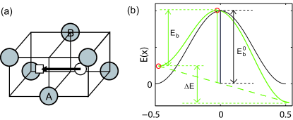
Figure 1: (a) In the non-interacting model $E_{b}$ depends only on whether cations $A$ and $B$ are Zr or Y. $E_{b}=0.58$, $1.29$ or $1.86$ eV if within pair $A$-$B$ there are 0, 1, or 2 Y cations Krishna . Filled circles represent cations, open circle represents oxygen anion, and open square represents oxygen vacancy. (b) In our interacting model, the energy difference $\Delta E$ between the initial and final state is assumed to modify the energy profile of vacancy jump by superimposing a linear function.

A fundamental input to the kMC simulation is the energy barriers for vacancy jumps, $E_{b}$, which depends on the ionic configurations around the jumping vacancy. In a previous model Krishna , $E_{b}$ is assumed to depend only on the chemical species of the two cations closest to the jumping vacancy, as shown in Fig. 1(a). Because the energy barrier of every jump equals that of the reverse jump, one can show that all metastable states in this model must have identical energy. Hence we will refer to it as the non-interacting model. Experimental and computational data have suggested that interactions play an important role in ionic conduction Stapper ; Pietrucci . To account for interactions, we use the kinetically resolved activation (KRA) model Ven1 ; Ven2 , in which $E_{b}=f(E_{b}^{0},\Delta E)$, where $E_{b}^{0}$ is the “kinetically resolved” barrier when the two metastable states happen to have identical energy, and $\Delta E$ is the energy difference between the two states. We take the energy barriers in the non-interacting model Krishna as our $E_{b}^{0}$. The function $f$ is often approximated by $E_{b}=E_{b}^{0}-\Delta E/2$ Ven1 ; Ven2 . Here we use a slightly better approximation for function $f$ by assuming that the energy landscape between the two metastable states has a sinusoidal shape when $\Delta E=0$, and is modified by a linear term when $\Delta E\neq 0$ Supple . Hence our task of specifying the energy barrier $E_{b}$ is reduced to an accurate description of the energy difference $\Delta E$.

Because the ionic interactions in YSZ are long ranged, they can only be captured accurately by DFT calculations in relatively large supercells. It is impossible to perform DFT calculations for all ionic configurations sampled by the kMC simulation. Instead, we use the cluster expansion method (CEM) to limit the necessary number of DFT calculations. In CEM, every metastable state in the kMC simulation can be uniquely mapped to a spin configuration $\{s_{i}\}$ of an Ising model Predith . The energy as a function of ionic configuration can be expressed by a cluster expansion Tepesch

$$E(\{s_{i}\})=\sum_{\alpha}V_{\alpha}\phi_{\alpha}(\{s_{i}\})$$ (1)

where $V_{\alpha}$ is called effective cluster interaction (ECI) for cluster $\alpha$, and $\phi_{\alpha}=\prod_{i\in\alpha}s_{i}$ is the cluster function involving all spin variables belonging to cluster $\alpha$. Eq. (1) is used to compute the energy of any metastable state encountered by the kMC simulation, prior to which the ECI coefficients $V_{\alpha}$’s are fitted to a DFT data set.

To construct the ab initio database for the fitting, we performed DFT calculations for 140 randomly chosen ionic configurations within a $3[100]\times 3[010]\times 3[001]$ YSZ supercell, using the Vienna Ab-initio Simulation Package (VASP) VASP . This supercell contains 108 cation sites (Zr or Y) and 216 anion sites (O or V_O) and is significantly larger than previous studies Krishna ; Predith , in order to accurately account for long range Coulombic and elastic interactions. K-point sampling is limited to the $\Gamma$-point considering the large size of supercell. The volume and the shape of the supercell are allowed to relax together with the ionic positions. A high energy cut-off of 520 eV is used to avoid Pulay stress. Each ionic configuration takes $\sim 10^{4}$ CPU-hours to be fully relaxed.

The number of clusters needs to be significantly truncated for robust fitting, otherwise the cluster expansion model can be overly-adapted to the fitted data set Rosen . First, we only keep the clusters in which any two spins are separated by less than 1.5$a_{0}$, where $a_{0}$ is the lattice parameter of YSZ. Second, we only keep clusters that involve up to 3 spins. Accounting for the translational and rotational symmetries, 192 independent clusters survive this truncation. For further truncation, a Monte Carlo algorithm is used to select $n_{c}$ clusters out of 192 possible clusters by minimizing the cross validation score Predith . To measure the predictive power of CEM, we separate the DFT data into two sets. Set I contains 100 data points and are used to fit the ECI’s. Set II contains 40 data points are used to benchmark the CEM’s predictions. The root mean square difference between the DFT energies and the CEM’s predictions per cation in Set I and Set II are defined as the error of fitting and the error of prediction, respectively.

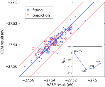
Figure 2: (color online) The 140 data points are divided into two sets: set I contains 100 data points ($\times$) and is used to fit CEM, set II contains 40 data points ($\circ$) and is not included in the fit. Energies predicted from CEM are plotted against energies computed from DFT using VASP, in units of eV per cation. The inset shows the effective binding energy between Y and oxygen vacancy predicted by CEM.

These two errors have different dependence on $n_{c}$. For example, when $n_{c}=97$, the error of fitting is $0.0006$ eV while the error of prediction is $0.012$ eV. The large difference between the two errors means that the fitted CEM has entirely lost its predictive power if $n_{c}$ is too large. Only when $n_{c}\leq 9$, both errors are the same, and decrease with increasing $n_{c}$. Hence, in this work, the optimal choice is $n_{c}=9$ Supple , where both the error of fitting and the error of prediction is $0.005$ eV, as shown in Fig. 2. This error is small enough for our kMC simulations and is smaller than a previous study Predith . To our knowledge this is the first time the predictive power of an interaction model for YSZ has been demonstrated by monitoring the error of prediction. Fig. 2(b) shows the effective binding energy between an Y ion and an oxygen vacancy predicted by the CEM model. The preference of the oxygen vacancy to the second nearest neighbor site of Y is clearly seen, consistent with previous experimental and theoretical works Krishna ; Rojana .

The fitted CEM allows us to compute the energy difference $\Delta E$ between the two states before and after a vacancy jump, which modifies the energy barrier $E_{b}$ of the jump. Using this energy barrier model, we performed kMC simulations in $3[100]\times 3[010]\times 3[001]$ YSZ supercells in which the doping concentration varies from $5\%$ to $13\%$. The ionic conductivity at each doping concentration is computed by averaging over 40 randomly generated Y distributions. As shown in Fig. 3(a), the ionic conductivity (at 1800 K) is maximum at 8-mol%, consistent with earlier experimental Ioffe ; Ikeda and theoretical results Krishna ; Rojana . Fig. 3(b) is the Arrhenius plot of ionic conductivity at 8mol% doping concentration. The predicted activation energy is 0.74eV at high $T$ and 0.85eV at low $T$, in much better agreement with experiments (0.85-1.0 eV)  Ikeda than the non-interacting model (0.59 eV) Krishna . The remaining difference with experiments may be due to the error in $E_{b}^{0}$ taken from Krishna . The neglect of activation entropy in vacancy jumps does not affect the conclusion because it does not change the slope of the Arrhenius plot.

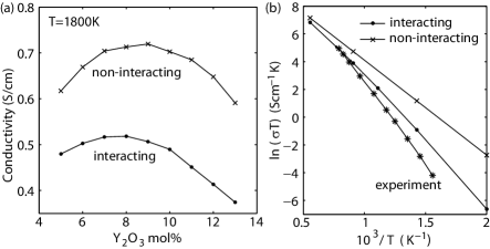
Figure 3: (a) Conductivity of YSZ single crystal predicted by kMC simulations at $T=1800$ K as a function of doping concentration. (b) Predicted temperature dependence of YSZ conductivity at 8-mol% doping concentration. Y dopant cations are assumed to be randomly distributed. Experimental data is reproduced from Ikeda .

The conductivity results shown in Fig. 3 are the averaged value over 40 random Y configurations, the standard deviation over which is about $19\%$ of the average. This indicates that the ionic conductivity is sensitive to the spatial distribution of Y cations and poses the question: what is the optimal Y distribution that maximizes ionic conductivity? To answer this question, we have performed kMC simulations for a variety of Y distributions, in which the Y cations are segregated into either spherical clusters, (001) layers, or [100] rods. The simulation results suggest two design principles that ultimately guide us to the optimal Y distribution.

When all Y cations in the supercell are segregated into a spherical cluster, the ionic conductivity is actually lower than the random distribution (by $27\%$ at $1800$ K), contrary to the prediction based on the non-interacting model Lee . This is because the interaction between Y cations and oxygen vacancies, as shown in Fig. 2, attracts the vacancies next to the cluster. To diffuse over long distances and contribute to the ionic conductivity, vacancies must detach from the Y clusters. This requires overcoming a binding energy of $\sim 0.12$ eV, which reduces the ionic conductivity.

Here the reduction of ionic conductivity is caused by the increase of spatial variation of the potential energy. Based on this result, we can formulate design principle I: the optimal Y distribution should minimize the energy variation of the metastable states as oxygen vacancies jump along the conduction direction. In this work, we focus on conduction along the [100] (i.e. $x$) direction. A promising candidate structure is to have Y cations segregated into planes, so that each (001) cation layer is either completely filled by Y, or completely filled by Zr. Due to translational invariance, the potential energy from cation-vacancy interaction remains constant after an oxygen vacancy jumps in the [100] direction . The layered structure can be fabricated using thin film deposition techniques such as PLD Chao .

Unfortunately, the layered structure also has a lower conductivity than the random distribution (by $59\%$ at $1800$ K). This is surprising because one might expect enhanced conductivity, as the non-interacting model would predict, due to the existence of Y-free channels. The reduction in conductivity is caused by the segregation of oxygen vacancies to the two anionic layers immediately next to the Y layer. Because there is always a first nearest neighbor (1nn) Y, vacancy diffusion in this layer experiences a high energy barrier (with $E_{b}^{0}=1.29$ eV). Given that vacancies prefer to be the second nearest neighbors (2nn) of Y, as shown in Fig. 2, it is somewhat surprising that the vacancies segregate to the nearest anionic layer. This problem is resolved by noticing that when the vacancy becomes the 1nn of two Y cations, it becomes the 2nn to four Y cations on the same cation layer. This result motivates our design principle II: the optimal Y distribution should not induce a high oxygen vacancy density in the first nearest neighbor sites of any Y cations.

It turns out that the design principles I and II can be simultaneously satisfied when Y cations are segregated into [100] lines. When Y lines are well separated from each other, kMC simulations show that the oxygen vacancy density is peaked at 2nn sites surrounding the Y lines. To enhance conductivity, we would like to pack more Y lines per unit volume in order to enhance the overall vacancy density. But when the distance between Y lines becomes too small, oxygen vacancies start to occupy 1nn sites around Y, deteriorating the ionic conductivity.

We examined a variety of 2D structures formed by [100] Y-segregated lines. The optimal structure at $1800$ K is a square lattice with periodicity 1.5$a_{0}$ in $y$ and $z$ directions (structure A). Interestingly, the optimal structure at $500$ K is different; it is a rectangular lattice with periodicity 1.5$a_{0}$ and 2$a_{0}$ in $y$ and $z$ directions, respectively (structure B). In both structures, the vacancy concentration is high in fast diffusing channels ($E_{b}^{0}=0.58$ eV) away from 1nn sites of Y, see Fig. 4(a).

Fig. 4(b) plots the temperature dependence of conductivity for structures A and B. Their activation energy is around $\sim 0.6$ eV, significantly lower than the random distribution. Compared with the random Y distribution (at 8mol%), the ionic conductivity of structure A is enhanced by a factor of 1.35 at 1800 K, 11 at 500 K and 86 at 300 K. For structure B, the enhancement factor is 22 at 500 K and 532 at 300 K. This result provides a theoretical upper limit of ionic conductivity that can be achieved by rearranging dopants in YSZ.

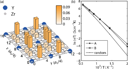
Figure 4: (color) (a) Vacancy distribution in structure B at $T=500$ K - blue and gray circles indicate Y and Zr, respectively. Darker color in the orange columns corresponds to higher vacancy concentration. (b) Temperature dependence of the conductivity at different Y distributions. Random Y distribution corresponds to a doping concentration of 8mol%.

In summary, we have developed an ab-initio based kMC model of the vacancy diffusion in bulk YSZ that accurately accounts for the ionic interactions. The predicted ionic conductivity shows much better agreement with experiments regarding the temperature dependence than the non-interacting model. The model predicts strong dependence of ionic conductivity on the spatial distribution of dopant cations. The maximum conductivity is reached when Y cations are arranged into a rectangular superlattice of [100] lines. Fabrication of this structure is challenging, but may be feasible with novel deposition techniques. The method presented here can be easily applied to other solid electrolytes, in which the optimal dopant microstructure may be different from that in YSZ and may be easier to synthesize.

This work is partly supported by the DOE/SciDAC project on Quantum Simulations of Materials and Nanostructures. E. Lee acknowledges support from the Samsung Scholarship Foundation. F. B. Prinz acknowledges support from the DOE-EFRC: CNEEC (Award No. DE-SC0001060)

References

- (1) R. O’Hayre, S.-W. Cha, W. Colella, and F. B. Prinz Fuel Cell Fundamentals, (Wiley, New York, 2006), Ch. 7.
- (2) S. Hui et al., J. Power Sources, 172, 493 (2007).
- (3) B. Steele and A. Heinzel, Nature 414, 345 (2001).
- (4) G. Knöner et al., Proc. Nat’l. Acad. Sci. USA 100, 3870 (2003).
- (5) R. Souza et al., Phys. Chem. Chem. Phys. 10, 2067 (2008).
- (6) N. Sata et al., Nature 408, 946 (2000).
- (7) I. Kosaki et al., Solid State Ionics 176, 1319 (2005).
- (8) J. Garcia-Barriocanal et al., Science 321, 676 (2008).
- (9) N. Schichtel et al., Phys. Chem. Chem. Phys. 11, 3043 (2009).
- (10) G. Stapper et al., Phys. Rev. B 59, 797 (1999).
- (11) F. Pietrucci et al., Phys. Rev. B 78, 094301 (2008).
- (12) C. Chao, Y. Kim, and F. Prinz, Nano Lett. 9, 3626 (2009).
- (13) T. Sayle, S. Parker, and D. Sayle, J. Mater. Chem. 16, 1067 (2006).
- (14) T. Pennycook et al., Phys. Rev. Lett. 104, 115901 (2010).
- (15) E. Lee, F. Prinz, and W. Cai, Electrochemistry Comm. 12, 223 (2010).
- (16) R. Krishnamurthy et al., J. Am. Ceram. Soc. 87, 1821 (2004).
- (17) R. Pornprasertsuk et al., J. Appl. Phys. 98, 103513 (2005).
- (18) A. Predith et al., Phys. Rev. B 77, 144104 (2008).
- (19) A. B. Bortz, M. H. Kalos, and J. L. Lebowitz, J. Comput. Phys. 17, 10 (1975).
- (20) A. Van der Ven et al., Phys. Rev. B 64, 184307 (2001).
- (21) A. Van der Ven and G. Ceder, Phys. Rev. Lett. 94, 045901 (2005).
- (22) P. D. Tepesch, G. D. Garbulsky, and G. Ceder, Phys. Rev. Lett. 74, 2272 (1995).
- (23) G. Kresse and J. Furthmüller, Phys. Rev. B 54, 11169 (1996)
- (24) J. Rosen et al., Comput. Optim. Appl. 17, 329 (2000)
- (25) A. I. Ioffe, D. Rutman, and S. Karpachov, Electrochim. Acta. 23, 141 (1978).
- (26) S. Ikeda et al., J. Mater. Sci. 20, 4593 (1985).
- (27) See supplementary materials.