INSTITUT NATIONAL DE RECHERCHE EN INFORMATIQUE ET EN AUTOMATIQUE

Efficient Bayesian Inference for Generalized Bradley-Terry Models
François Caron — Arnaud DoucetN° 7445
November 2010

Abstract: The Bradley-Terry model is a popular approach to describe probabilities of the possible outcomes when elements of a set are repeatedly compared with one another in pairs. It has found many applications including animal behaviour, chess ranking and multiclass classification. Numerous extensions of the basic model have also been proposed in the literature including models with ties, multiple comparisons, group comparisons and random graphs. From a computational point of view, Hunter, (2004) has proposed efficient iterative MM (minorization-maximization) algorithms to perform maximum likelihood estimation for these generalized Bradley-Terry models whereas Bayesian inference is typically performed using MCMC (Markov chain Monte Carlo) algorithms based on tailored Metropolis-Hastings (M-H) proposals. We show here that these MM algorithms can be reinterpreted as special instances of Expectation-Maximization (EM) algorithms associated to suitable sets of latent variables and propose some original extensions. These latent variables allow us to derive simple Gibbs samplers for Bayesian inference. We demonstrate experimentally the efficiency of these algorithms on a variety of applications.

Key-words: Bradley–Terry model, data augmentation, EM algorithm, Gibbs sampler, maximum likelihood estimation, MCMC algorithms, MM algorithm, Plackett–Luce model

Inférence bayésienne pour les modèles de Bradley-Terry généralisés

Résumé : Le modèle de Bradley-Terry est une approche populaire pour décrire les résultats possibles lorsque des éléments d’un ensemble sont mis en comparaison par paire. Il a trouvé de nombreuses applications incluant le comportement animal, le classement de joueurs d’échecs et la classification multi-classes. Plusieurs extensions du modèle classique ont été proposées dans la littérature afin de prendre en compte des matchs nuls, des comparaisons multiples et des comparaisons entre groupes. D’un point de vue computationel, Hunter, (2004) a proposé des algorithmes MM (minorization-maximization) itératifs efficaces pour l’estimation du maximum de vraisemblance dans les modèles de Bradley-Terry généralisés, tandis que l’inférence bayésienne est réalisée à l’aide d’algorithmes MCMC (Markov chain Monte Carlo) basées sur des lois de proposition Metropolis-Hastings (M-H) adaptées. Nous montrons que ces algorithmes MM peuvent être réinterprétés comme des instances d’algorithmes EM (Expectation-Maximization) associés à des ensembles de variables latentes. Ces variables latentes nous permettent de dériver des algorithmes de Gibbs simples pour l’inférence bayésiennes. Nous démontrons expérimentalement l’efficacité de ces algorithmes sur plusieurs applications.

Mots-clés : Modèle de Bradley-Terry, Algorithme EM, Echantillonneur de Gibbs, Estimation par maximum de vraisemblance, algorithmes MCMC, algorithme MM, Modèle de Plackett-Luce

1 Introduction

Consider a set of $K$ elements. These elements are repeatedly compared with one another in pairs. For two elements $i$ and $j$ of this set, Bradley and Terry, (1952) suggested the following model

$$\Pr(i\text{ beats }j)=\frac{\lambda_{i}}{\lambda_{i}+\lambda_{j}}$$ (1)

where $\lambda_{l}>0$ is a parameter associated to element $l\in\left\{1,2,\ldots,K\right\}$ that represents its skill rating and we denote $\lambda:=\left\{\lambda_{i}\right\}_{i=1}^{K}$.

This model has found numerous applications. As mentioned in (Hunter, , 2004), as early as 1976, a published bibliography on paired comparisons includes several hundred entries (Davidson and Farquhar, , 1976). For example, it has been adopted by the World Chess Federation and the European Go Federation to rank players and it is a standard approach to build multiclass classifiers based on the output of binary classifiers (Hastie and Tibshirani, , 1998). Various extensions have been proposed to handle home advantage (Agresti, , 1990), draws (Rao and Kupper, , 1967), multiple (Plackett, , 1975; Luce, , 1959) and team comparisons (Huang et al., , 2006). In particular, the popular extension to multiple comparisons, named the Plackett-Luce model (Plackett, , 1975; Luce, , 1959), defines a prior distribution over permutations and has been used for ranking of multiple individuals and for choice models (Luce, , 1977). The monographs of David, (1988) and Diaconis, (1988, Chap. 9) provide detailed discussions on the statistical foundations of these models.

For the basic Bradley-Terry model (1), it is possible to find the maximum likelihood (ML) estimate of the skill ratings $\lambda$ using a simple iterative procedure (Zermelo, , 1929; Hunter, , 2004). Lange et al., (2000) established that this procedure is a specific case of the general class of algorithms referred to as MM algorithms. Generally speaking, MM algorithms use surrogate minimizing functions of the log-likelihood to define an iterative procedure converging to a local maximum. EM algorithms are thus just a special case of MM algorithms. An excellent survey of the MM approach and its applications can be found in (Lange et al., , 2000). Hunter, (2004) further derived MM algorithms for generalized Bradley-Terry models and established sufficient conditions under which these algorithms are guaranteed to converge towards the ML estimate.

Recently several authors have proposed to perform Bayesian inference for (generalized) Bradley-Terry models (Adams, , 2005; Gormley and Murphy, , 2009; Görür et al., , 2006; Guiver and Snelson, , 2009). The resulting posterior density is typically not tractable and needs to be approximated. An Expectation-Propagation method is developed in (Guiver and Snelson, , 2009); this yields an approximation of the posterior which can be computed quickly and might be suitable for very large scale applications. However, it relies on a functional approximation of the posterior and the convergence properties of this algorithm are not well-understood. M-H algorithms have been proposed in (Adams, , 2005; Gormley and Murphy, , 2009; Görür et al., , 2006). Gormley and Murphy, (2009) suggested a carefully designed proposal distribution, though it can perform poorly in some scenarios as demonstrated in section 6.

Our contribution here is three-fold. First, we show that by introducing suitable sets of latent variables, the MM algorithms proposed by Hunter, (2004) for the basic Bradley-Terry model and its generalizations to take into account home advantage, ties and multiple comparisons can be reinterpreted as standard EM algorithms. We believe that this non-trivial reinterpretation is potentially fruitful for statisticians who usually like thinking in terms of latent variables. Note that the latent variables introduced here differ from the ones introduced in the standard Thurstonian interpretation of the Bradley-Terry model (Diaconis, , 1988, Chap. 9) and lead to more efficient algorithms as discussed in section 2. Second, using similar ideas, we propose original EM algorithms for some recent generalizations of the Bradley-Terry model including group comparisons and random graphs. Third, based on the sets of latent variables introduced to derive these EM algorithms, we propose Gibbs samplers to perform Bayesian inference in this important class of models. To the best of our knowledge, no Gibbs sampler has ever been proposed in this context. These algorithms have the great advantage of allowing us to bypass the design of proposal distributions for M-H updates and we demonstrate experimentally that they perform very well.

The rest of this paper is organized as follows. In section 2, we consider the basic Bradley-Terry model (1). Based on the introduction of a suitable set of latent variables, we present an EM reinterpretation of the MM algorithm presented by Hunter, (2004) for Maximum a Posteriori (MAP) parameter estimation and an original data augmentation algorithm to sample from the posterior. In section 3, various standard extensions of the Bradley-Terry model allowing for home advantage, ties and competition between teams are described. EM algorithms and original Gibbs sampling schemes are proposed. The Plackett-Luce model (Plackett, , 1975; Luce, , 1959), a very popular generalization of the Bradley-Terry model for multiple comparisons, is presented in section 4. Algorithms applicable to further extensions of the Bradley-Terry model to choice models, random graphs and classification are presented in section 5. In section 6, these algorithms are applied to the NASCAR 2002 dataset and to chess competition data.

2 Bradley-Terry model

Suppose we have observed a number of statistically independent pairwise comparisons among $K$ individuals. We denote by $D$ the associated data. Let also $w_{ij}$ denote the number of comparisons where $i$ beats $j$ and $n_{ij}=w_{ij}+w_{ji}$ the total number of comparisons between $i$ and $j$. Based on the Bradley-Terry model (1), the log-likelihood function is given by

$$\ell(\lambda) =\sum_{1\leq i\neq j\leq K}\text{ }w_{ij}\log\lambda_{i}-w_{ij}\log(\lambda_{i}+\lambda_{j})$$

$$=\sum_{1\leq i\neq j\leq K}\text{ }w_{ij}\log\lambda_{i}-\sum_{1\leq i<j\leq K}\text{ }n_{ij}\log(\lambda_{i}+\lambda_{j})$$

where the notation $1\leq i\neq j\leq K$ is an abusive notation to denote the set $\left\{\left(i,j\right)\in\left\{1,...,K\right\}^{2}\right.$ $\left.\text{ such that }i\neq j\right\}$ and $1\leq i<j\leq K$ stands for $\left\{\left(i,j\right)\in\left\{1,...,K\right\}^{2}\text{ such that }i<j\right\}$.

We seek to introduce latent variables which are such that the resulting complete log-likelihood admits a simple form. It is well-known that the Bradley-Terry model enjoys the following Thurstonian interpretation (Diaconis, , 1988, Chap. 9): for each pair $1\leq i<j\leq K$ and for each associated pair comparison $k=1,\ldots,n_{ij}$, let $Y_{ki}\sim\mathcal{E}(\lambda_{i})$ and $Y_{kj}\sim\mathcal{E}(\lambda_{j})$ where $\mathcal{E}\left(\varsigma\right)$ is the exponential distribution of rate parameter $\varsigma$ then

$$\Pr(Y_{ki}<Y_{kj})=\frac{\lambda_{i}}{\lambda_{i}+\lambda_{j}}.$$

These latent variables can be interpreted as arrival times and the individual with the lowest arrival time wins. These latent variables would allow us to define EM and data augmentation algorithms. However, if we only introduce for each pair $i,j$ the sum of the lowest arrival times

$$Z_{ij}=\sum_{k=1}^{n_{ij}}\min(Y_{kj},Y_{ki})\sim\mathcal{G(}n_{ij},\lambda_{i}+\lambda_{j})$$

instead of $\left\{Y_{ki},Y_{kj}\right\}$ for $k=1,\ldots,n_{ij}$, then the resulting complete log-likelihood remains simple. Here $\mathcal{G}\left(\alpha,\beta\right)$ denote the Gamma distribution of shape $\alpha$ and inverse scale $\beta$. As the fraction of missing information is reduced, this leads to faster rates of convergence for the resulting EM and data augmentation algorithms (Liu, , 2001, Chap. 6). We will essentially proceed similarly to introduce latent variables for generalized Bradley-Terry models.

To summarize, for $1\leq i<j\leq K$ such that $n_{ij}>0$, we introduce the latent variables $Z=\left\{Z_{ij}\right\}$ which are such that

$$p\left(\left.z\right|D,\lambda\right)={\displaystyle\prod\limits_{1\leq i<j\leq K|n_{ij}>0}}\mathcal{G}(z_{ij};n_{ij},\lambda_{i}+\lambda_{j})$$ (2)

The resulting complete data log-likelihood is given by

$$\ell(\lambda,z)=\sum_{1\leq i\neq j\leq K|w_{ij}>0}w_{ij}\log\lambda_{i}-\sum_{1\leq i<j\leq K|n_{ij}>0}(\lambda_{i}+\lambda_{j})z_{ij}+(n_{ij}-1)\log z_{ij}-\log\Gamma(n_{ij})$$ (3)

where $\Gamma$ is the Gamma function.

If we assign additionally a prior to $\lambda$ such that

$$p\left(\lambda\right)={\displaystyle\prod\limits_{i=1}^{K}}\mathcal{G}(\lambda_{i};a,b)$$ (4)

as in (Gormley and Murphy, , 2009; Guiver and Snelson, , 2009) then we can maximize the resulting log-posterior using the EM algorithm which proceeds as follows at iteration $t$:

$$\lambda^{(t)}=\underset{\lambda}{\arg\max}\text{ }Q(\lambda,\lambda^{\left(t-1\right)}).$$ (5)

We have

$$Q(\lambda,\lambda^{\ast}) =\mathbb{E}_{\left.Z\right|D,\lambda^{\ast}}\left[\ell(\lambda,Z)\right]+\log\text{ }p\left(\lambda\right)$$ (6)

$$\equiv\sum_{i=1}^{K}\left(a-1+w_{i}\right)\log\lambda_{i}-b\lambda_{i}-\sum_{1\leq i<j\leq K}(\lambda_{i}+\lambda_{j})\frac{n_{ij}}{\lambda_{i}^{\ast}+\lambda_{j}^{\ast}}$$

with “$\equiv$” meaning “equal up to terms independent of the first argument of the $Q$ function” and $w_{i}=\sum_{j=1,j\neq i}^{K}w_{ij}$ is the number of wins of element $i$. Using (5), it follows that

$$\lambda_{i}^{(t)}=\frac{a-1+w_{i}}{b+\sum_{j\neq i}\frac{n_{ij}}{\lambda_{i}^{(t-1)}+\lambda_{j}^{(t-1)}}}.$$ (7)

For $a=1$ and $b=0$, the MAP and ML estimates coincide. In this case (6) is exactly the minorizing function of the MM algorithm proposed in (Hunter, , 2004, Eq. (10)) and thus the MM algorithm is given by (7).

Based on the same latent variables, we present a simple data augmentation algorithm for sampling from the posterior distribution $p\left(\left.\lambda,z\right|D\right)\propto p\left(\lambda\right)\exp\left(\ell(\lambda,z)\right)$. By construction, we can update $Z$ conditional upon $\lambda$ using (2) and the conditional for $\lambda$ given $Z$ can be expressed easily so that the data augmentation sampler at iteration $t$ proceeds as follows:

• For $1\leq i<j\leq K$ s.t. $n_{ij}>0$, sample

  $$Z_{ij}^{(t)}|D,\lambda^{(t-1)}\sim\mathcal{G}(n_{ij},\lambda_{i}^{(t-1)}+\lambda_{j}^{(t-1)}).$$

• For $i=1,\ldots,K,$ sample

  $$\lambda_{i}^{(t)}|D,Z^{(t)}\sim\mathcal{G(}a+w_{i},b+\sum_{i<j|n_{ij}>0}Z_{ij}^{(t)}+\sum_{i>j|n_{ij}>0}Z_{ji}^{(t)}).$$

3 Generalized Bradley-Terry models

3.1 Home advantage

Consider now that the pairwise comparisons are modeled using the Bradley-Terry model with “home-field advantage” (Agresti, , 1990) where

$$\Pr(i\text{ beats }j)=\left\{\begin{array}[c]{ll}\frac{\theta\lambda_{i}}{\theta\lambda_{i}+\lambda_{j}}&\text{if }i\text{ is home,}\\ \frac{\lambda_{i}}{\lambda_{i}+\theta\lambda_{j}}&\text{if }j\text{ is home.}\end{array}\right.$$

The parameter $\theta$, $\theta>0$, measures the strength of the home-field advantage ($\theta>1$) or disadvantage ($\theta<1$). Let $a_{ij}$ be the number of times that $i$ is at home and beats $j$ and $b_{ij}$ is the number of times that $i$ is at home and loses to $j$.

The log-likelihood of the skill ratings $\lambda$ and $\theta$ is given by

$$\ell(\lambda,\theta)=c\log\theta+\sum_{i=1}^{K}w_{i}\log\lambda_{i}-\sum_{1\leq i\neq j\leq K}n_{ij}\log(\theta\lambda_{i}+\lambda_{j})$$

where $n_{ij}=a_{ij}+b_{ij}$ is the number of times $i$ plays at home against $j$, $c=\sum_{1\leq i\neq j\leq K}a_{ij}$ is the total number of home-field wins and $w_{i}$ is the total number of wins of element $i$.

For $1\leq i\neq j\leq K$ such that $n_{ij}>0$, let us introduce the latent variables $Z=\left\{Z_{ij}\right\}$ which are such that

$$p\left(\left.z\right|D,\lambda\right)={\displaystyle\prod\limits_{1\leq i\neq j\leq K|n_{ij}>0}}\mathcal{G}(z_{ij};n_{ij},\theta\lambda_{i}+\lambda_{j}).$$ (8)

The associated complete data log-likelihood is given by

$$\ell(\lambda,\theta,z)=c\log\theta+\sum_{i=1}^{K}w_{i}\log\lambda_{i}-\sum_{1\leq i\neq j\leq K|n_{ij}>0}(\theta\lambda_{i}+\lambda_{j})z_{ij}+\log\Gamma\left(n_{ij}\right).$$

Using independent priors for $\lambda$ and $\theta$, i.e. $p\left(\lambda,\theta\right)=p\left(\lambda\right)p\left(\theta\right)$, where $p\left(\lambda\right)$ is defined as (4) and

$$\theta\sim\mathcal{G}(a_{\theta},b_{\theta}),$$ (9)

then we can maximize the resulting posterior using the EM algorithm

$$\left(\lambda^{(t)},\theta^{\left(t\right)}\right)=\text{ }\underset{\left(\lambda,\theta\right)}{\arg\max}\text{ }Q(\left(\lambda,\theta\right),\left(\lambda^{\left(t-1\right)},\theta^{\left(t-1\right)}\right))$$

where we have

$$Q(\left(\lambda,\theta\right),\left(\lambda^{\ast},\theta^{\ast}\right)) =\mathbb{E}_{Z|D,\lambda^{\ast},\theta^{\ast}}\left[\ell(\lambda,\theta,Z)\right]+\log\text{ }p\left(\lambda,\theta\right)$$

$$\equiv\left(a_{\theta}-1+c\right)\log\theta-b_{\theta}\theta+\sum_{i=1}^{K}\left(a-1+w_{i}\right)\log\lambda_{i}-b\sum_{i=1}^{K}\lambda_{i}-\sum_{1\leq i\neq j\leq K}n_{ij}\frac{\theta\lambda_{i}+\lambda_{j}}{\theta^{\ast}\lambda_{i}^{\ast}+\lambda_{j}^{\ast}}.$$

We obtain

$$\lambda_{i}^{(t)} =\frac{a-1+w_{i}}{b+\sum_{1\leq i\neq j\leq K}\text{ }\left\{\frac{\theta^{(t-1)}n_{ij}}{\theta^{(t-1)}\lambda_{i}^{(t-1)}+\lambda_{j}^{(t-1)}}+\frac{n_{ji}}{\theta^{(t-1)}\lambda_{j}^{(t-1)}+\lambda_{i}^{(t-1)}}\right\}}\text{ for }i=1,\ldots,K,$$

$$\theta^{(t)} =\frac{a_{\theta}-1+c}{b_{\theta}+\sum_{1\leq i\neq j\leq K}\frac{n_{ij}\text{ }\lambda_{i}^{(t)}}{\theta^{(t-1)}\lambda_{i}^{(t-1)}+\lambda_{j}^{(t-1)}}}.$$

For $a=a_{\theta}=1$ and $b=b_{\theta}=0$, i.e. if we use flat priors, this EM algorithm is similar to the MM algorithm proposed in (Hunter, , 2004, pp. 389).

Using the same latent variables, we can sample from the posterior distribution of $\left(\lambda,\theta,Z\right)$ using the Gibbs sampler which updates iteratively $Z,$ $\lambda$ and $\theta$ as follows at iteration $t$:

• For $1\leq i\neq j\leq K$ s.t. $n_{ij}>0$, sample

  $$Z_{ij}^{(t)}|D,\lambda^{(t-1)},\theta^{(t-1)}\sim\mathcal{G}\left(n_{ij},\theta^{(t-1)}\lambda_{i}^{(t-1)}+\lambda_{j}^{(t-1)}\right).$$

• For $i=1,\ldots,K,$ sample

  $$\lambda_{i}^{(t)}|D,\theta^{(t-1)},Z^{(t)}\sim\mathcal{G}\left(a+w_{i},b+\theta^{\left(t-1\right)}\sum_{j\neq i|n_{ij}>0}Z_{ij}^{(t)}+\sum_{j\neq i|n_{ij}>0}Z_{ji}^{\left(t\right)}\right).$$

• Sample

  $$\theta^{\left(t\right)}|D,\lambda^{(t)},Z^{(t)}\sim\mathcal{G}\left(a_{\theta}+c,b_{\theta}+\sum_{i=1}^{K}\lambda_{i}^{\left(t\right)}\sum_{j\neq i|n_{ij}>0}Z_{ij}^{\left(t\right)}\right).$$

3.2 Model with ties

If we now want to allow for ties in pairwise comparisons, we can use the following model proposed by Rao and Kupper, (1967)

$$\Pr(i\text{ beats }j) =\frac{\lambda_{i}}{\lambda_{i}+\theta\lambda_{j}},$$

$$\Pr(i\text{ ties }j) =\frac{(\theta^{2}-1)\lambda_{i}\lambda_{j}}{(\lambda_{i}+\theta\lambda_{j})(\theta\lambda_{i}+\lambda_{j})}$$

where $\theta>1$. The log-likelihood function for $\left(\lambda,\theta\right)$ is given by

$$\ell(\lambda,\theta) =\sum_{1\leq i\neq j\leq K}w_{ij}\log\frac{\lambda_{i}}{\lambda_{i}+\theta\lambda_{j}}+\frac{t_{ij}}{2}\log\frac{(\theta^{2}-1)\lambda_{i}\lambda_{j}}{(\theta\lambda_{i}+\lambda_{j})(\lambda_{i}+\theta\lambda_{j})}$$

$$=\sum_{1\leq i\neq j\leq K}s_{ij}\log\frac{\lambda_{i}}{\lambda_{i}+\theta\lambda_{j}}+\frac{t_{ij}}{2}\log(\theta^{2}-1)$$

where $t_{ij}=t_{ji}$ is the number of ties between $i$ and $j$ and $s_{ij}=w_{ij}+t_{ij}$.

For $1\leq i\neq j\leq K$ such that $s_{ij}>0$, let us introduce the latent variables $Z=\left\{Z_{ij}\right\}$ which are such that

$$p\left(\left.z\right|D,\lambda\right)={\displaystyle\prod\limits_{1\leq i\neq j\leq K|s_{ij}>0}}\mathcal{G}(z_{ij};s_{ij},\lambda_{i}+\theta\lambda_{j})$$

which yields the following complete log-likelihood

$$\ell(\lambda,\theta,z)=T\log(\theta^{2}-1)+\sum_{1\leq i\neq j\leq K|s_{ij}>0}s_{ij}\log\lambda_{i}-(\lambda_{i}+\theta\lambda_{j})z_{ij}+(s_{ij}-1)\log z_{ij}-\log\Gamma(s_{ij})$$

where $T=\frac{1}{2}\sum_{1\leq i\neq j\leq K}t_{ij}$ is the total number of ties. If we adopt for $\theta$ a flat improper prior on $\left[1,\infty\right)$ and we select $p\left(\lambda\right)$ as (4) then we obtain

$$Q(\left(\lambda,\theta\right),\left(\lambda^{\ast},\theta^{\ast}\right)) =\mathbb{E}_{Z|D,\lambda^{\ast},\theta^{\ast}}\left[\ell(\lambda,\theta,Z)\right]+\log\text{ }p\left(\lambda,\theta\right)$$

$$\equiv T\log(\theta^{2}-1)+\sum_{1\leq i\neq j\leq K}s_{ij}\left(\log\lambda_{i}-\frac{\lambda_{i}+\theta\lambda_{j}}{\lambda_{i}^{\ast}+\theta^{\ast}\lambda_{j}^{\ast}}\right)+\sum_{i=1}^{K}\left(a-1\right)\log\lambda_{i}-b\lambda_{i}$$

and we recover once again the minorizing function in (Hunter, , 2004, pp. 389-390) for $a=1$ and $b=0$. This can be maximized using the following procedure

• For $i=1,\ldots,K,$ set

  $$\lambda_{i}^{(t)}=\left(a-1+\sum_{j\neq i}s_{ij}\right)\left[b+\sum_{j\neq i}\frac{s_{ij}}{\lambda_{i}^{(t-1)}+\theta^{(t-1)}\lambda_{j}^{(t-1)}}+\frac{\theta^{(t-1)}s_{ji}}{\theta^{(t-1)}\lambda_{i}^{(t-1)}+\lambda_{j}^{(t-1)}}\right]^{-1}\text{.}$$

• Set

  $$\theta^{(t)}=\frac{1}{2c^{(t)}}+\sqrt{1+\frac{1}{4c^{(t)\text{ }2}}}$$

  where

  $$c^{(t)}=\sum_{1\leq i\neq j\leq K}\frac{s_{ij}\lambda_{j}^{(t)}}{\lambda_{i}^{(t-1)}+\theta^{(t-1)}\lambda_{j}^{(t-1)}}\text{.}$$

Using the same latent variables, we can sample from the posterior distribution of $\left(\lambda,\theta,Z\right)$ using the following Gibbs sampler which updates iteratively $Z,$ $\lambda$ and $\theta$ as follows at iteration $t$:

• For $1\leq i\neq j\leq K$ s.t. $s_{ij}>0$, sample

  $$Z_{ij}^{\left(t\right)}|D,\lambda^{(t-1)},\theta^{(t-1)}\sim\mathcal{G}\left(s_{ij},\lambda_{i}^{\left(t-1\right)}+\theta^{(t-1)}\lambda_{j}^{\left(t-1\right)}\right).$$

• For $i=1,\ldots,K$, sample

  $$\lambda_{i}^{(t)}|D,\theta^{(t-1)},Z^{(t)}\sim\mathcal{G}\left(a+\sum_{j\neq i}s_{ij},b+\sum_{j\neq i|s_{ij}>0}Z_{ij}^{\left(t\right)}+\theta^{(t-1)}\sum_{j\neq i|s_{ij}>0}Z_{ji}^{\left(t\right)}\right).$$

• Sample

  $$\theta^{\left(t\right)}|D,\lambda^{(t)},Z^{(t)}\sim p(\theta|D,\lambda^{(t)},Z^{\left(t\right)})$$

  where

  $$p(\theta|D,Z,\lambda)\propto(\theta^{2}-1)^{T}\exp\left(-\sum_{1\leq i\neq j\leq K|s_{ij}>0}Z_{ij}\text{ \ }\theta\right)1_{\theta>1}.$$ (10)

It is possible to sample from (10) exactly. By performing a change of variable $\overline{\theta}=\theta-1$, we obtain

$$p(\overline{\theta}|D,Z,\lambda)\propto(\overline{\theta}^{2}+2\overline{\theta})^{T}\exp\left(-\sum_{1\leq i\neq j\leq K|s_{ij}>0}Z_{ij}\text{ \ }\overline{\theta}\right)$$

which is a mixture of Gamma distributions.

3.3 Group comparisons

Consider now that we have $n$ pairwise comparisons betweem teams. For each comparison $i=1,\ldots,n$, let $T_{i}^{+}\subset\{1,\ldots,K\}$ be the winning team and $T_{i}^{-}\subset\{1,\ldots,K\}$ the losing team where $T_{i}^{+}\cap T_{i}^{-}=\varnothing$ and $T_{i}=T_{i}^{+}\cup T_{i}^{-}$. Recently Huang et al., (2006) have proposed the following model

$$\Pr(T_{i}^{+}\text{ beats }T_{i}^{-})=\frac{\sum_{j\in T_{i}^{+}}\lambda_{j}}{\sum_{j\in T_{i}}\lambda_{j}}\text{.}$$ (11)

The log-likelihood function for $\lambda$ is thus given by

$$\ell(\lambda)=\sum_{i=1}^{n}\log\left(\sum_{j\in T_{i}^{+}}\lambda_{j}\right)-\log\left(\sum_{j\in T_{i}}\lambda_{j}\right)\text{.}$$

For $i=1,...,n$ we introduce the latent variables $Z=\left\{Z_{i}\right\}$ and $C=\left\{C_{i}\right\}$ such that

$$p\left(\left.z,c\right|D,\lambda\right)=p\left(\left.z\right|D,\lambda\right)P\left(\left.c\right|D,\lambda\right)$$

with

$$p\left(\left.z\right|D,\lambda\right) ={\displaystyle\prod\limits_{i=1}^{n}}\mathcal{E}\left(z_{i};\sum_{j\in T_{i}}\lambda_{j}\right),$$

$$\Pr\left(\left.c\right|D,\lambda\right) ={\displaystyle\prod\limits_{i=1}^{n}}\frac{\lambda_{c_{i}}}{\sum_{j\in T_{i}^{+}}\lambda_{j}}\text{ with }c_{i}\in T_{i}^{+}$$

where $\mathcal{E}\left(x;\alpha\right)$ is the exponential density of argument $x$ and parameter $\alpha$. It follows that the complete log-likelihood is given by

$$\ell(\lambda,z,c)=\sum_{i=1}^{n}\log\lambda_{c_{i}}-\left(\sum_{j\in T_{i}}\lambda_{j}\right)z_{i}.$$

The $Q$ function associated to the EM algorithm is given by

$$Q(\lambda,\lambda^{\ast}) =\mathbb{E}_{Z,C|D,\lambda^{\ast}}\left[\ell(\lambda,Z,C)\right]+\log\text{ }p\left(\lambda\right)$$

$$\equiv\sum_{i=1}^{n}\sum_{j\in T_{i}^{+}}\log\lambda_{j}\frac{\lambda_{j}^{\ast}}{\sum_{k\in T_{i}^{+}}\lambda_{k}^{\ast}}-\frac{\sum_{j\in T_{i}}\lambda_{j}}{\sum_{j\in T_{i}}\lambda_{j}^{\ast}}+\sum_{k=1}^{K}\left(a-1\right)\log\lambda_{k}-b\lambda_{k}$$

$$\equiv\sum_{k=1}^{K}\left(a-1+\lambda_{k}^{\ast}\sum_{i=1}^{n}\frac{\alpha_{ik}}{\sum_{j\in T_{i}^{+}}\lambda_{j}^{\ast}}\right)\log\lambda_{k}-\lambda_{k}\left(b+\sum_{i=1}^{n}\frac{\gamma_{ik}}{\sum_{j\in T_{i}}\lambda_{j}^{\ast}}\right)$$

where $\alpha_{ik}=1$ if $k\in T_{i}^{+}$ and $0$ otherwise and $\gamma_{ik}=1$ if $k\in T_{i}$ and $0$ otherwise. It follows that the EM update is given by

$$\lambda_{k}^{\left(t\right)}=\frac{a-1+\lambda_{k}^{\ast}\sum_{i=1}^{n}\frac{\alpha_{ik}}{\sum_{j\in T_{i}^{+}}\lambda_{j}^{\left(t-1\right)}}}{b+\sum_{i=1}^{n}\frac{\gamma_{ik}}{\sum_{j\in T_{i}}\lambda_{j}^{\left(t-1\right)}}}.$$

Using the same latent variables, we obtain a data augmentation sampler to sample from $p\left(\left.\lambda,z,c\right|D\right)$ by iteratively sampling $\left(Z,C\right)$ and $\lambda.$ This proceeds as follows at iteration $t$:

• For $i=1,...,n$, sample

  $$Z_{i}^{\left(t\right)}|D,\lambda^{(t-1)}\sim\mathcal{E}\left(\sum_{j\in T_{i}}\lambda_{j}^{\left(t-1\right)}\right),$$

      

• For $k=1,\ldots,K$, sample

  $$\lambda_{k}^{(t)}|D,Z^{(t)},C^{(t)}\sim\mathcal{G}\left(a+\sum_{i=1}^{n}\delta_{k,C_{i}^{\left(t\right)}},b+\sum_{i=1}^{n}\gamma_{ik}Z_{i}^{\left(t\right)}\right)$$

  where $\delta_{u,v}=1$ if $u=v$ and $0$ otherwise.

4 Multiple comparisons

We now consider the popular Plackett-Luce model (Luce, , 1959; Plackett, , 1975) which is an extension of the Bradley-Terry model to comparisons involving more than two elements. Assume that $p_{i}\leq K$ individuals are ranked for comparison $i$ where $i=1,...,n$. We write $\rho_{i}=(\rho_{i1},\ldots,\rho_{ip_{i}})$ where $\rho_{i1}$ is the first individual, $\rho_{i2}$, the second, etc. The Plackett-Luce model assumes

$$\Pr(\rho_{i}|\lambda)=\prod_{j=1}^{p_{i}}\frac{\lambda_{\rho_{ij}}}{\sum_{k=j}^{p_{i}}\lambda_{\rho_{ik}}}=\prod_{j=1}^{p_{i}-1}\frac{\lambda_{\rho_{ij}}}{\sum_{k=j}^{p_{i}}\lambda_{\rho_{ik}}}.$$ (12)

For $i=1,\ldots,n$ and $j=1,\ldots,p_{i}-1$, we introduce the following latent variables $Z=\left\{Z_{ij}\right\}$

$$p\left(\left.z\right|D,\lambda\right)=\prod_{i=1}^{n}\prod_{j=1}^{p_{i}-1}\mathcal{E(}z_{ij};\sum_{k=j}^{p_{i}}\lambda_{\rho_{ik}})$$

which leads to the complete log-likelihood

$$\ell(\lambda,z)=\sum_{i=1}^{n}\sum_{j=1}^{p_{i}-1}\text{ }\log\lambda_{\rho_{ij}}-\left(\sum_{k=j}^{p_{i}}\lambda_{\rho_{ik}}\right)z_{ij}.$$

The $Q$ function associated to the EM algorithm is given by

$$Q(\lambda,\lambda^{\ast}) =\mathbb{E}_{Z|D,\lambda^{\ast}}\left[\ell(\lambda,Z)\right]+\log\text{ }p\left(\lambda\right)$$

$$\equiv\sum_{i=1}^{n}\sum_{j=1}^{p_{i}-1}\log\lambda_{\rho_{ij}}-\frac{\sum_{k=j}^{p_{i}}\lambda_{\rho_{ik}}}{\sum_{k=j}^{p_{i}}\lambda_{\rho_{ik}}^{\ast}}+\sum_{k=1}^{K}\text{ }\left(a-1\right)\log\lambda_{k}-b\lambda_{k}$$

which is once again equivalent to the majorizing function in (Hunter, , 2004, pp. 398) for $a=1,$ $b=0$. It follows that the EM algorithm is given at iteration $t$ by

$$\lambda_{k}^{(t)}=(a-1+w_{k})\left[b+\sum_{i=1}^{n}\left(\sum_{j=1}^{p_{i}-1}\frac{\delta_{ijk}}{\sum_{k=j}^{p_{i}}\lambda_{\rho_{ik}}^{(t-1)}}\right)\right]^{-1}$$

where $w_{k}$ is the number of rankings where the $k^{\text{th}}$ individual is not in the last ranking position and $\delta_{ijk}$ is defined as

$$\delta_{ijk}=\left\{\begin{array}[c]{ll}1&\text{if }k\in\{\rho_{ij},\ldots,\rho_{ip_{j}}\}\\ 0&\text{otherwise}\end{array}\right.$$

i.e. $\delta_{ijk}$ is the indicator of the event that individual $k$ receives a rank no better than $j$ in the $i^{\text{th}}$ ranking.

To sample from $p\left(\left.\lambda,z\right|D\right)$, we can use the following data augmentation sampler. At iteration $t$, this proceeds as follows:

• For $i=1,...,n$, for $j=1,\ldots,p_{i}-1$, sample

  $$Z_{ij}^{\left(t\right)}|D,\lambda^{\left(t-1\right)}\sim\mathcal{E}(\sum_{k=j}^{p_{i}}\lambda_{\rho_{ik}}^{\left(t-1\right)}).$$

• For $k=1,\ldots,K$, sample

  $$\lambda_{k}^{\left(t\right)}|D,Z^{\left(t\right)}\sim\mathcal{G}(a+w_{k},b+\sum_{i=1}^{n}\sum_{j=1}^{p_{i}-1}\delta_{ijk}Z_{ij}^{\left(t\right)}).$$

Using exactly the same augmentation, EM and Gibbs samplers can be defined for further extensions of these models such as mixtures of Plackett-Luce models (Gormley and Murphy, , 2008).

5 Discussion

5.1 Identifiability

Consider the basic Bradley-Terry model and its extensions to group comparisons and multiple comparisons. Let us define

$$\Lambda=\sum_{i=1}^{K}\lambda_{i}\text{ \ and }\pi_{i}=\frac{\lambda_{i}}{\Lambda}$$

and write $\pi:=\left\{\pi_{i}\right\}_{i=1}^{K}$. The likelihood is invariant to a rescaling of the vector $\lambda$ so the parameter $\Lambda$ is not likelihood-identifiable and

$$p(\pi,\Lambda|D)=p(\left.\pi\right|D)p(\Lambda).$$

From (4), it follows that $\pi\sim\mathcal{D}(a,\ldots,a)$ where $\mathcal{D}$ is the Dirichlet distribution and $\Lambda\sim\mathcal{G}(Ka,b)$, hence

$$\Lambda^{MAP}=\frac{aK-1}{b}.$$

To improve the mixing of the MCMC algorithms in this context, an additional sampling step can be added where we normalize the current parameter estimate $\lambda^{\left(t\right)}$ and then rescale them randomly using a prior draw for $\Lambda$.

• For $i=1,\ldots,K$, set $\lambda_{i}^{\ast(t)}=\frac{\lambda_{i}^{(t)}}{\sum_{j=1}^{K}\lambda_{j}^{(t)}}\Lambda^{(t)}$ where $\Lambda^{(t)}\sim\mathcal{G}(Ka,b)$.

This step can drastically improve the mixing of the Markov chain. However, if we are only interested in the normalized values $\pi$ of $\lambda$ then this additional step is useless.

As an alternative, it is also possible to consider an EM algorithm for the basic Bradley-Terry model which does not require the introduction of a scale parameter. Assume $\pi\sim\mathcal{D}(a,\ldots,a)$ and let us introduce latent variables $M_{ij}$, $C_{ij}=(C_{ij1},\ldots,C_{ijM_{ij}})$ for $1\leq i\neq j\leq K$ such that $n_{ij}>0$

$$M_{ij} \sim NB(n_{ij},\pi_{i}+\pi_{j}),$$

$$\Pr\left(C_{ijk}=l\right) =\frac{\pi_{l}}{\sum_{n\neq i,j}\pi_{n}}\text{ for }k=1,\ldots M_{ij}\text{ and }l\neq i,j$$

where $NB(r,p)$ is the negative binomial distribution. The complete log-likelihood is given by

$$\ell(\pi,m,c)=\sum_{i=1}^{K}\sum_{j=1,j\neq i}^{K}w_{ij}\log\pi_{i}+\sum_{i=1}^{K}\sum_{j=1,j\neq i}^{K}\sum_{k\neq i,j}\left[\log\binom{n_{ij}+m_{ij}-1}{n_{ij}-1}+r_{ijk}\log\pi_{k}\right]$$

where $r_{ijk}$ is the number of $c_{ijl},l=1,\ldots,m_{ij}$ that take value $k$. Omitting the terms independent of $\pi$, the $Q$ function is given by

$$Q(\pi,\pi^{\ast}) =\mathbb{E}_{M|D,\pi^{\ast}}\left[\mathbb{E}_{C|D,M,\pi^{\ast}}\left[\ell(\pi,M,C)\right]\right]+\log\text{ }p\left(\pi\right)$$

$$\equiv\mathbb{E}_{M|D,\pi^{\ast}}\left[\sum_{i=1}^{K}\sum_{j=1,j\neq i}^{K}w_{ij}\log\pi_{i}+\sum_{i=1}^{K}\sum_{j=1,j\neq i}^{K}\sum_{k\neq i,j}\log\binom{n_{ij}+M_{ij}-1}{n_{ij}-1}+M_{ij}\frac{\pi_{k}^{\ast}}{\sum_{l\neq i,j}\pi_{l}^{\ast}}\log\pi_{k}\right]$$

$$+\log\text{ }p\left(\pi\right)$$

$$\equiv\sum_{i=1}^{K}\sum_{j=1,j\neq i}^{K}w_{ij}\log\pi_{i}+\sum_{i=1}^{K}\sum_{j=1,j\neq i}^{K}\sum_{k\neq i,j}n_{ij}\frac{\pi_{k}^{\ast}}{\pi_{i}^{\ast}+\pi_{j}^{\ast}}\log\pi_{k}+\left(a-1\right)\sum_{i=1}^{K}\log\pi_{k}+C$$

$$\equiv\sum_{k=1}^{K}(w_{k}+\pi_{k}^{\ast}\sum_{i=1,i\neq k}^{K}\sum_{j=1,j\neq i,k}^{K}\frac{n_{ij}}{\pi_{i}^{\ast}+\pi_{j}^{\ast}}\log\pi_{k})+\left(a-1\right)\sum_{i=1}^{K}\log\pi_{k}+C$$

where $C$ is a term independent of $\pi$. It follows that the EM update is given by

$$\pi_{k}^{(t)}\propto a-1+w_{k}+\pi_{k}^{(t-1)}\sum_{i=1,i\neq k}^{K}\sum_{j=1,j\neq i,k}^{K}\frac{n_{ij}}{\pi_{i}^{(t-1)}+\pi_{j}^{(t-1)}}$$

with $\sum_{k=1}^{K}\pi_{k}^{\left(t\right)}=1.$ Although the above EM algorithm does not rely on unidentifiable scaling parameters, it suffers from a slow convergence rate. When $\pi_{k}$ takes small values, $\sum_{i\neq k}\sum_{j\neq k}\frac{n_{ij}}{\pi_{i}+\pi_{j}}$ is large and it slows down the convergence of the EM algorithm. The same augmentation can be used to define a Gibbs sampler, but the same slow mixing issues arise for the Markov chain.

5.2 Hyperparameter estimation

The prior (4) is specified by the hyperparameters $a$ and $b$. However, the inverse scale parameter $b$ is not likelihood identifiable so there is no point assigning a prior to it. However it might be interesting to set a prior $p(a)$ on $a$ and estimate it from the data. Given $\lambda$, we have

$$p\left(\left.a\right|\lambda\right)\propto p\left(a\right)\underset{l_{1}\left(a\right)}{\underbrace{\left(b^{K}\prod_{i=1}^{K}\lambda_{i}\right)^{a}\text{\ }}}\text{ }\underset{l_{2}(a)}{\underbrace{\Gamma^{-K}(a)}}.$$

It is possible to sample from this density using auxiliary variables $U_{1},U_{2}$ defined on $\left(0,\infty\right)$ as described in (Damien et al., , 1999). We introduce

$$p\left(\left.a,u_{1},u_{2}\right|\lambda\right)\propto p\left(a\right)\mathbb{I}\left\{u_{1}<l_{1}\left(a\right)\right\}\mathbb{I}\left\{u_{2}<l_{2}\left(a\right)\right\}.$$

A Gibbs sampler can now be implemented to sample from $p\left(\left.a,u_{1},u_{2}\right|\lambda\right)$. We can directly sample from the full conditionals of $U_{1}$ and $U_{2}$

$$\left.U_{1}\right|\lambda\sim\mathcal{U}\left(0,l_{1}\left(a\right)\right),\text{ \ }\left.U_{2}\right|\lambda\sim\mathcal{U}\left(0,l_{2}\left(a\right)\right)$$

where $\mathcal{U}\left(\alpha,\beta\right)$ is the uniform distribution on $\left(\alpha,\beta\right)$. The full conditional of $a$ given $u_{1},u_{2}$ is given by

$$p\left(\left.a\right|\lambda,u_{1},u_{2}\right)\propto p\left(a\right)\mathbb{I}_{A_{1}\cap A_{2}}\left(a\right)$$

where

$$A_{i}=\left\{a:l_{i}\left(a\right)>u_{i}\right\}.$$

Alternatively we can update $a$ using a M-H random walk on $\log(a)$. We can propose $a^{\star}=\exp(\sigma_{a}^{2}z)a$ where $z\sim\mathcal{N}(0,1)$ and $a^{\star}$ is accepted with probability

$$\min\left\{1,\frac{p(a^{\star})}{p(a)}\left(\frac{\Gamma(a)}{\Gamma(a^{\star})}\right)^{K}\left(b^{K}\prod_{i=1}^{K}\lambda_{i}\right)^{a^{\star}-a}\right\}.$$

5.3 Further extensions

5.3.1 Random graphs with a given degree sequence

A model closely related to Bradley-Terry has been proposed for undirected random graphs with $K$ vertices (Holland and Leinhardt, , 1981; Chatterjee et al., , 2010; Park and Newman, , 2004). In this model, the degree sequence $(d_{1},\ldots,d_{K})$ of a given graph, where $d_{i}$ is the degree of node $i$, is supposed to capture all the information in the graph. It can be formalized by saying that the degree sequence is a sufficient statistic for a probability distribution on graphs (Chatterjee et al., , 2010).

In this model an edge is inserted between vertices $i$ and $j$ for $1\leq i<j\leq K$ with probability

$$\frac{\lambda_{i}\lambda_{j}}{1+\lambda_{i}\lambda_{j}}$$

where $\lambda_{k}>0$ for $k\in\{1,\ldots,K\}$. Let $r_{ij}=1$ if there is an edge between $i$ and $j$ and $0$ otherwise. Given the observations $D=\left\{r_{ij}\right\}_{1\leq i<j\leq K}$, the log-likelihood function for $\lambda$ is given by

$$\ell(\lambda)=\sum_{1\leq i<j\leq K}r_{ij}\log\left(\lambda_{i}\lambda_{j}\right)-\log\left(1+\lambda_{i}\lambda_{j}\right).$$

We introduce the following latent variables $Z=\left\{Z_{ij}\right\}_{1\leq i<j\leq K}$ such that

$$p\left(\left.z\right|D,\lambda\right)={\displaystyle\prod\limits_{1\leq i<j\leq K}}\mathcal{E}(z_{ij};\lambda_{i}+\frac{1}{\lambda_{j}})\text{.}$$

The complete log-likelihood is given by

$$\ell(\lambda,z)=\sum_{1\leq i<j\leq K}r_{ij}\log\lambda_{i}-(1-r_{ij})\log\lambda_{j}-(\lambda_{i}+\frac{1}{\lambda_{j}})z_{ij}$$

The $Q$ function associated to the EM algorithm is given by

$$Q(\lambda,\lambda^{\ast}) =\mathbb{E}_{Z|D,\lambda^{\ast}}\left[\ell(\lambda,Z)\right]+\log\text{ }p\left(\lambda\right)$$

$$\equiv\sum_{i=1}^{K}\log\lambda_{i}\left[\left(a-1\right)+\sum_{j>i}r_{ij}-\sum_{j<i}(1-r_{ij})\right]-\lambda_{i}\left(b+\sum_{j>i}\frac{1}{\lambda_{i}^{\ast}+\frac{1}{\lambda_{j}^{\ast}}}\right)-\frac{1}{\lambda_{i}}\sum_{j<i}\frac{1}{\lambda_{j}^{\ast}+\frac{1}{\lambda_{i}^{\ast}}}.$$

Solving $\partial Q(\lambda,\lambda^{\ast})/\partial\lambda_{i}=0$ requires solving a quadratic equation. For sake of brevity, we do not present these details here.

Once again, we can define a data augmentation sampler to sample from $p\left(\left.\lambda,z\right|D\right)$ by iteratively sampling $Z$ and $\lambda.$ This proceeds as follows at iteration $t$:

• For $1\leq i<j\leq K$, sample

  $$\left.Z_{ij}^{\left(t\right)}\right|D,\lambda^{(t-1)}\sim\mathcal{E(}\lambda_{i}^{\left(t-1\right)}+\frac{1}{\lambda_{j}^{\left(t-1\right)}}).$$

• For $i=1,...,K$, sample

  $$\lambda_{i}^{\left(t\right)}|D,Z^{\left(t\right)}\sim\mathcal{GIG}\left(2(\sum_{j>i}Z_{ij}^{\left(t\right)}+b),2\sum_{j<i}Z_{ij}^{\left(t\right)},a+\sum_{j>i}r_{ij}-\sum_{j<i}(1-r_{ij})\right).$$

Here $\mathcal{GIG}\left(\alpha,\beta,\gamma\right)$ denotes the generalized inverse Gaussian distribution (see e.g. (Barndorff-Nielsen and Shephard, , 2001)) whose density for an argument $x$ is proportional to

$$x^{\gamma-1}\exp\left\{-\left(\alpha x+\beta/x\right)/2\right\}.$$

Algorithms to sample exactly from this distribution are available.

5.3.2 Choice models

Other extensions of the Bradley-Terry model are the choice models introduced by Restle, (1961) and Tversky, 1972a ; Tversky, 1972b in psychology; see also (Wickelmaier and Shmidt, , 2004; Görür et al., , 2006). In these models, we are given a set of $n$ elements. To each element $i$ is associated a set of $K$ features represented by a binary vector $f_{i}\in\{0,1\}^{K}$. The probability that element $i$ is chosen over element $j$ is given by

$$\pi_{ij}=\frac{\sum_{k=1}^{K}\lambda_{k}f_{ik}(1-f_{jk})}{\sum_{k=1}^{K}\lambda_{k}f_{ik}(1-f_{jk})+\sum_{k=1}^{K}\lambda_{k}f_{jk}(1-f_{ik})}$$

where $\lambda_{k}>0$ is a weight representing the importance of feature $k$. The term $\sum_{k=1}^{K}\lambda_{k}f_{ik}(1-f_{jk})$ corresponds to the sum of the weights of features possessed by object $i$ but not object $j$. EM and Gibbs algorithms can be derived by following the same construction as with group comparisons.

5.3.3 Classification model

Let consider the following original model for categorical data analysis

$$\Pr(Y_{i}=k) =\frac{\sum_{j=1}^{p}\exp(X_{ij})\lambda_{kj}}{\sum_{l=1}^{K}\sum_{j=1}^{p}\exp(X_{ij})\lambda_{lj}}$$

$$=\frac{\exp(X_{i})^{T}\lambda_{k}}{\sum_{l=1}^{K}\exp(X_{i})^{T}\lambda_{l}}$$ (13)

where $X_{i}\in\mathbb{R}^{p}$ is a vector of covariates and $\lambda_{k}\in\mathbb{R}_{+}^{p}$ for $k=1,\ldots,K$. This model could be used as an alternative to the multinomial logit model (Agresti, , 1990). By introducing latent variables $Z_{i}\sim\mathcal{E}\left(\sum_{l=1}^{K}\exp(X_{i})^{T}\lambda_{l}\right)$, we can define EM and Gibbs algorithms resp. to maximize the posterior distribution of the parameters $\lambda_{k}$ and sample from it when the prior is given by (4).

6 Experimental results

In all the above models, the parameter $b$ is just a scaling parameter on $\lambda_{k}$. As the likelihood is invariant to a rescaling of the $\lambda_{k}$, this parameter does not have any influence on inference. Hence to ensure that the MAP estimate satisfies $\sum_{k=1}^{K}\widehat{\lambda}_{k}=1$, we set $b=Ka-1$ henceforth as explained in section 5. We demonstrate our algorithms on one synthetic and two real-world data sets.

6.1 Synthetic Data

We first study the Plackett-Luce model, comparing experimentally the mixing properties of the Gibbs sampler relative to a slightly modified version of the M-H algorithm proposed by Gormley and Murphy, (2009). In this latter paper, the authors propose to update the skill parameters simultaneously using the following proposal distribution at iteration $t$

$$\text{for }i=1,\ldots,K\text{, }\lambda_{i}^{\star}\sim\mathcal{G}\left(a+w_{k},b+\sum_{i=1}^{n}\left(\sum_{j=1}^{p_{i}-1}\frac{\delta_{ijk}}{\sum_{k=j}^{p}\lambda_{\rho_{ik}}^{(t-1)}}\right)\right)$$

We simulated $500$ dataset of $n$ rankings of $K=4$ individuals, for various values of $n$ with $a=5$. For each dataset, 10,000 iterations of the Gibbs sampler presented in section 4 were run. The sample lag-1 autocorrelation was then computed for the four skill parameters. For a given sample size $n$, the mean value over skill parameters and simulated data is reported on Figure 1 together with 90% confidence bounds. The algorithm of Gormley and Murphy, (2009) performs reasonably well when the sample size is large, which is the case for the voting data they considered, but poorly for small sample sizes.

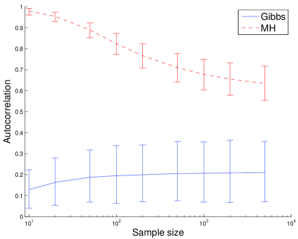
Figure 1: Sample lag-1 autocorrelation as a function of the sample size $n$ for the Gibbs sampler and a modified version of the M-H algorithm of Gormley and Murphy (2009).

6.2 Nascar 2002 dataset

NASCAR is the primary sanctioning body for stock car auto racing in the United States. Each race involves 43 drivers. During the 2002 season, 87 different drivers participated in 36 races. Some drivers participated in all of the races while others participated in only one. We propose to apply the Plackett-Luce model with gamma prior on the parameters. The NASCAR dataset has been studied by Hunter, (2004), who noted that the MLE cannot be found for the original data set as four drivers placed last in each race they entered, and therefore had to be removed. This does not need to be done if we follow a Bayesian approach. We focus here on predicting the outcome of the next race based on the previous ones, starting from race 5; i.e. we predict the results of race 6 based on the MAP estimates obtained with the first 5 races, then the results of race 7 based on the MAP estimated obtained with the first 6 races, etc. For each race, we compute the test log-likelihood using the MAP estimates. The mean value and 90% confidence bounds are represented in Figure 2 w.r.t. the value of $a$. The EM algorithm was initialized using $(\lambda_{1}^{\left(0\right)},\ldots,\lambda_{83}^{\left(0\right)})=(\frac{1}{83},\ldots,\frac{1}{83})$.

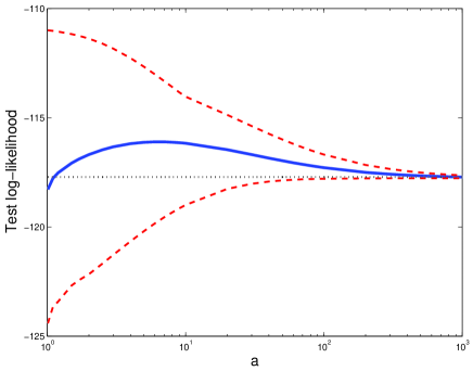
Figure 2: Test log-likelihood on the Nascar 2002 dataset. From race 5 to 35, we compute the log-likelihood of the next race based on the MAP estimates. Mean and 90% interval of the log-likelihood is represented w.r.t. to the parameter $a$. The straight line represents the test log-likelihood obtained with a uniform prior.

The Gibbs sampler was also applied to the same dataset. The skill parameters were initialized at the same value, and the parameter $a$ was assigned a flat improper prior and sampled as described in section 5. We ran 50,000 iterations with 2,000 burn-in. As detailed in Section 5, only the normalized weights $\pi_{i}$ are likelihood identifiable. Skill ratings are usually represented on the real line, and we use the following one-to-one mapping $\beta_{i}=\log\pi_{i}-\log 1/83$. The marginal posterior densities of the reparameterized skill ratings for the first four drivers according to their average place are reported in Figure 3. The Bayesian approach can effectively capture the uncertainty in the skill ratings of the drivers. ML and MMSE (minimum mean squared error) estimates together with standard deviations are reported in Table 1 for the first ten and last ten drivers according to average place.

Table 1: Top ten and bottom ten drivers according to average place, along with ML and MMSE estimates of the skill parameters in $\beta$ space. Standard deviations are also provided.

		Average	MLE	MMSE	Standard
Driver	Races	place	estimate	estimate	Deviation
P. Jones	1	4.00	2.74	0.11	0.48
S. Pruett	1	6.00	2.21	0.10	0.48
M. Martin	36	12.17	0.67	0.79	0.17
T. Stewart	36	12.61	0.42	0.60	0.17
R. Wallace	36	13.17	0.65	0.78	0.17
J. Johnson	36	13.50	0.53	0.68	0.17
S. Marlin	29	13.86	0.33	0.49	0.19
M. Bliss	1	14.00	0.82	0.04	0.48
J. Gordon	36	14.06	0.33	0.53	0.17
K. Busch	36	14.06	0.24	0.46	0.17
…
C. Long	2	40.50	-1.73	-0.67	0.46
C. Fittipaldi	1	41.00	-1.85	-0.51	0.50
H. Fukuyama	2	41.00	-2.17	-0.81	0.50
J. Small	1	41.00	-1.94	-0.60	0.51
M. Shepherd	5	41.20	-1.86	-1.05	0.39
K. Shelmerdine	2	41.50	-1.73	-0.72	0.46
A. Cameron	1	42.00	-1.41	-0.44	0.49
D. Marcis	1	42.00	-1.38	-0.43	0.49
D. Trickle	3	42.00	-1.72	-0.87	0.42
J. Varde	1	42.00	-1.55	-0.48	0.50

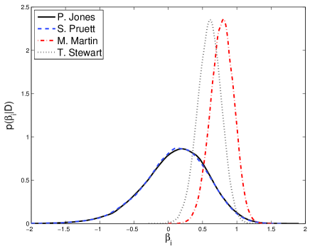
Figure 3: Marginal posterior distribution for the modified skill ratings $\beta_{i}$ of the first 4 drivers according to their average place. P. Jones and S. Pruett only participated in 1 race each, while M. Martin and T. Stewart participated in 36 races.

6.3 Chess data

Rating the skills of chess players is of major practical interest. It allows organizers of a tournament to avoid having strong players playing against each other at early stages, or to restrict the tournament to players with skills above a given threshold. The international chess federation adopted the so-called “Elo” system which is based on the Bradley-Terry model (Elo, , 1978). For historical considerations about the rating system in chess, the reader should refer to Glickman, (1995).

We consider here game-by-game chess results over 100 months, consisting of 65,053 matches between 8631 players. The outcome of each game is either win (+1), tie (+0.5) or loss (0). We estimate the parameters of the Bradley-Terry model with ties presented in section 3.2 on the first 95 months and then predict the outcome of the games of the last 5 months. The hyperparameters for the tie parameter $\theta$ are set to $a_{\theta}=1,$ $b_{\theta}=0$. Given the large sample size, it is not possible to sample from Eq. (10) as the number of elements in the mixture is very large. We therefore use a M-H step with a normal random walk proposal of standard deviation $0.1$. The mean squared error is reported for predictions based on MAP estimates and full Bayesian predictive based on the Gibbs sampler outcomes, for different values of the hyperparameter $a$. EM and Gibbs samplers were initialized at $(\lambda_{1}^{\left(0\right)},\ldots,\lambda_{8631}^{\left(0\right)})=(\frac{1}{8631},\ldots,\frac{1}{8631})$ and $\theta^{\left(0\right)}=1,5$. The Gibbs samplers were run with 10,000 iterations and 1,000 burn-in iterations. The results are reported in Figure 4. The results demonstrate the benefit of penalizing the skill rating parameters and the improvement brought up by a full Bayesian analysis. In Figure 5 we also report the autocorrelation function associated to the parameter $\theta$ and the skill parameters with largest mean values. The Markov chain displays good mixing properties.

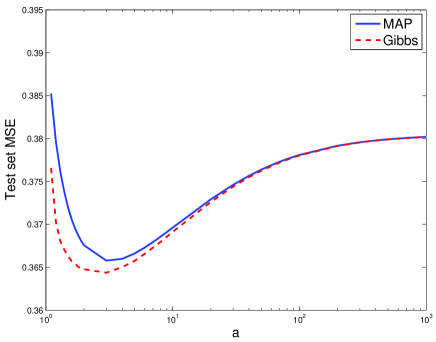
Figure 4: Test mean square error on the chess dataset for different values of the parameter $a$. Based on an history of 95 months, we predict the outcome of the games of the last 5 months.

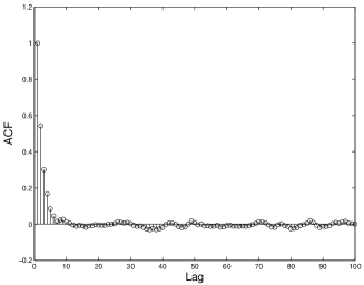
(a) Skill parameter with largest mean value

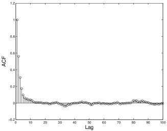
(b) Skill parameter with second largest mean value

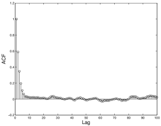
(c) Skill parameter with third largest mean value

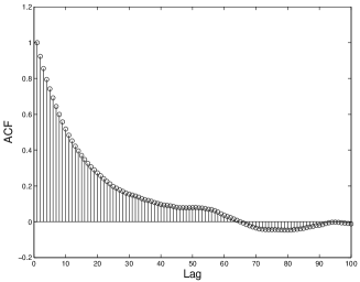
(d) Tie parameter $\theta$

Figure 5: Autocorrelation functions for (a-c) the three skill parameters with largest mean values and for (d) the parameter $\theta$. The fast decrease indicates that the Markov chain mixes well. The parameter $\theta$ is updated with a Metropolis-Hastings step which explains its relatively low mixing.

7 Conclusion

The Bradley-Terry model and its generalizations arise in numerous applications. We have shown here that most of the MM algorithms proposed in Hunter, (2004) can be reinterpreted as special cases of EM algorithms. Additionally we have proposed original EM algorithms for some recent generalizations of the Bradley-Terry models. Finally we have shown how the latent variables introduced to derive these EM algorithms lead straightforwardly to Gibbs sampling algorithms. These elegant MCMC algorithms mix experimentally well and outperform a recently proposed M-H algorithm.

Acknowledgment. The authors are grateful to Persi Diaconis for helpful discussions and pointers to references on the Plackett-Luce and random graph models and to Luke Bornn for helpful comments.

References

- Adams, (2005) Adams, E. (2005). Bayesian analysis of linear dominance hierarchies. Animal Behaviour, 69:1191–1201.
- Agresti, (1990) Agresti, A. (1990). Categorical Data Analysis. Wiley.
- Barndorff-Nielsen and Shephard, (2001) Barndorff-Nielsen, O. and Shephard, N. (2001). Non-Gaussian Ornstein-Uhlenbeck-based models and some of their uses in financial economics. Journal of the Royal Statistical Society B, 63:167–241.
- Bradley and Terry, (1952) Bradley, R. and Terry, M. (1952). Rank analysis of incomplete block designs. I. the method of paired comparisons. Biometrika, 39:324–345.
- Chatterjee et al., (2010) Chatterjee, S., Diaconis, P., and Sly, A. (2010). Random graphs with a given degree sequence. Technical report, Stanford University.
- Damien et al., (1999) Damien, P., Wakefield, J., and Walker, S. (1999). Gibbs sampling for Bayesian non-conjugate and hierarchical models by using auxiliary variables. Journal of the Royal Statistical Society B, 61:331–344.
- David, (1988) David, H. (1988). The method of paired comparisons. Oxford University Press.
- Davidson and Farquhar, (1976) Davidson, R. and Farquhar, P. (1976). A bibliography on the method of paired comparisons. Biometrics, 32:241–252.
- Diaconis, (1988) Diaconis, P. (1988). Group representations in probability and statistics, IMS Lecture Notes, volume 11. Institute of Mathematical Statistics.
- Elo, (1978) Elo, A. (1978). The rating of Chess Players, Past and present. Arco Pub.
- Glickman, (1995) Glickman, M. (1995). A comprehensive guide to chess ratings. Technical report, Department of Statistics, Boston University.
- Gormley and Murphy, (2008) Gormley, I. and Murphy, T. (2008). Exploring voting blocs with the Irish electorate: a mixture modeling approach. Journal of the American Statistical Association, 103:1014–1027.
- Gormley and Murphy, (2009) Gormley, I. and Murphy, T. (2009). A grade of membership model for rank data. Bayesian Analysis, 4:265–296.
- Görür et al., (2006) Görür, D., Jäkel, F., and Rasmussen, C. (2006). A choice model with infinitely many latent features. In International Conference on Machine Learning.
- Guiver and Snelson, (2009) Guiver, J. and Snelson, E. (2009). Bayesian inference for Plackett-Luce ranking models. In International Conference on Machine Learning.
- Hastie and Tibshirani, (1998) Hastie, T. and Tibshirani, R. (1998). Classification by pairwise coupling. Annals of Statistics, 26:451–471.
- Holland and Leinhardt, (1981) Holland, P. and Leinhardt, S. (1981). An exponential family of probability distributions for directed graphs. Journal of the American Statistical Association, 76:33–65.
- Huang et al., (2006) Huang, T.-K., Weng, R., and Lin, C.-J. (2006). Generalized Bradley-Terry models and multi-class probability estimates. Journal of Machine Learning Research, 7:85–115.
- Hunter, (2004) Hunter, D. (2004). MM algorithms for generalized Bradley-Terry models. The Annals of Statistics, 32:384–406.
- Lange et al., (2000) Lange, K., Hunter, D., and Yang, I. (2000). Optimization transfer using surrogate objective functions (with discussion). Journal of Computational and Graphical Statistics, 9:1–59.
- Liu, (2001) Liu, J. (2001). Monte Carlo Methods for Scientific Computing. Springer-Verlag: New York.
- Luce, (1959) Luce, R. (1959). Individual choice behavior: A theoretical analysis. Wiley.
- Luce, (1977) Luce, R. (1977). The choice axiom after twenty years. Journal of Mathematical Psychology, 15:215–233.
- Park and Newman, (2004) Park, J. and Newman, M. (2004). The statistical mechanics of networks. Physical Review E, 70:066117.
- Plackett, (1975) Plackett, R. (1975). The analysis of permutations. Applied Statistics, 24:193–202.
- Rao and Kupper, (1967) Rao, P. and Kupper, L. (1967). Ties in paired-comparison experiments: A generalization of the Bradley-Terry model. Journal of the American Statistical Association, 62:194–204.
- Restle, (1961) Restle, F. (1961). Psychology of judgement and choice. New-York: Wiley.
- (28) Tversky, A. (1972a). Choice by elimination. Journal of Mathematical Psychology, 9:341–367.
- (29) Tversky, A. (1972b). Elimination by aspects: a theory of choice. Psychological Review, 79:281–299.
- Wickelmaier and Shmidt, (2004) Wickelmaier, F. and Shmidt, C. (2004). A Matlab function to estimate choice model parameters from paired-comparison data. Behavior Research Methods, Instruments and Computers, 36:29–40.
- Zermelo, (1929) Zermelo, E. (1929). Die berechnung der turnier-ergebnisse als ein maximumproblem der wahrscheinlichkeitsrechnung. Math. Z., 29:436–460.