Online Expectation-Maximisation

Before entering into any more details about the methodological aspects, let’s discuss the motivations behind the association of the two phrases “online (estimation)” and “Expectation-Maximisation (algorithm)” as well as their pertinence in the context of mixtures and more general models involving latent variables.

The adjective online refers to the idea of computing estimates of model parameters on-the-fly, without storing the data and by continuously updating the estimates as more observations become available. In the machine learning literature, the phrase online learning has been mostly used recently to refer to a specific way of analysing the performance of algorithms that incorporate observations progressively (Césa-Bianchi and Lugosi,, 2006). We dot not refer here to this approach and will only consider the more traditional setup in which the objective is to estimate fixed parameters of a statistical model and the performance is quantified by the proximity between the estimates and the parameter to be estimated. In signal processing and control, the sort of algorithms considered in the following is often referred to as adaptive or recursive (Ljung and Söderström,, 1983, Benveniste et al.,, 1990). The word recursive is so ubiquitous in computer science that its use may be somewhat ambiguous and is not recommended. The term adaptive may refer to the type of algorithms considered in this chapter but is also often used in contexts where the focus is on the ability to track slow drifts or abrupt changes in the model parameters, which will not be our primary concerns.

Traditional applications of online algorithms involve situations in which the data cannot be stored, due to its volume and rate of sampling as in real-time signal processing or stream mining. The wide availability of very large datasets involving thousands or millions of examples is also at the origin of the current renewed interest in online algorithms. In this context, online algorithms are often more efficient —i.e., converging faster towards the target parameter value— and need fewer computer resource, in terms of memory or disk access, than their batch counterparts (Neal and Hinton,, 1999). In this chapter, we are interested in both contexts: when the online algorithm is used to process on-the-fly a potentially unlimited amount of data or when it is applied to a fixed but large dataset. We will refer to the latter context as the batch estimation mode.

Our main interest is maximum likelihood estimation and although we may consider adding a penalty term (i.e., Maximum A Posteriori estimation), we will not consider “fully Bayesian” methods which aim at sequentially simulating from the parameter posterior. The main motivation for this restriction is to stick to computationally simple iterations which is an essential requirement of successful online methods. In particular, when online algorithms are used for batch estimation, it is required that each parameter update can be carried out very efficiently for the method to be computationally competitive with traditional batch estimation algorithms. Fully Bayesian approaches —see, e.g., (Chopin,, 2002)— typically require Monte Carlo simulations even in simple models and raise some challenging stability issues when used on very long data records (Kantas et al.,, 2009).

This quest for simplicity of each of the parameter update is also the reason for focussing on the EM (Expectation-Maximisation) algorithm. Ever since its introduction by Dempster et al., (1977), the EM algorithm has been criticised for its often sub-optimal convergence behaviour and many variants have been proposed by, among others, Lange, (1995), Meng and Van Dyk, (1997). This being said, thirty years after the seminal paper by Dempster and his coauthors, the EM algorithm still is, by far, the most widely used inference tool for latent variable models due to its numerical stability and ease of implementation. Our main point here is not to argue that the EM algorithm is always preferable to other options. But the EM algorithm which does not rely on fine numerical tunings involving, for instance, line-searches, re-projections or pre-conditioning is a perfect candidate for developing online versions with very simple updates. We hope to convince the reader in the rest of this chapter that the online version of EM that is described here shares many of the attractive properties of the original proposal of Dempster et al., (1977) and provides an easy to implement and robust solution for online estimation in latent variable models.

Quite obviously, guaranteeing the strict likelihood ascent property of the original EM algorithm is hardly feasible in an online context. On the other hand, a remarkable property of the online EM algorithm is that it can reach asymptotic Fisher efficiency by converging towards the actual parameter value at a rate which is equivalent to that of the Maximum Likelihood Estimator (MLE). Hence, when the number of observations is sufficiently large, the online EM algorithm does becomes highly competitive and it not necessary to consider potentially faster-converging alternatives. When used for batch estimation, i.e., on a fixed large dataset, the situation is more contrasted but we will nonetheless show that the online algorithm does converge towards the maximum likelihood parameter estimate corresponding to the whole data. To achieve this result, one typically needs to scan the data set repeatedly. In terms of computing time, the advantages of using an online algorithm in this situation will typically depend on the size of the problem. For long data records however, this approach is certainly more recommendable than the use of the traditional batch EM algorithm and preferable to other alternatives considered in the literature.

The rest of this chapter is organised as follows. The first section is devoted to the modelling assumptions that are adopted throughout the chapter. In Section 2, we consider the large-sample behaviour of the traditional EM algorithm, insisting on the concept of the limiting EM recursion which is instrumental in the design of the online algorithm. The various aspects of the online EM algorithm are then examined in Sections 3 and 4.

Although the chapter is intended to be self-contained, we will nonetheless assume that the reader is familiar with the fundamental concepts of classical statistical inference and, in particular, with Fisher information, exponential families of distributions and maximum likelihood estimation, at the level of Lehmann and Casella, (1998), Bickel and Doksum, (2000) or equivalent texts.

1 Model and Assumptions

We assume that we are able to observe an independent sequence of identically distributed data $(Y_{t})_{t\geq 1}$, with marginal distribution $\pi$. An important remark is that we do not necessarily assume that $\pi$ corresponds to a distribution that is reachable by the statistical model that is used to fit the data. As discussed in Section 3.4 below, this distinction is important to analyse the use of the online algorithm for batch maximum-likelihood estimation.

The statistical models that we consider are of the missing-data type, with an unobservable random variable $X_{t}$ associated to each observation $Y_{t}$. The latent variable $X_{t}$ may be continuous or vector-valued and we will not be restricting ourselves to finite mixture models. Following the terminology introduced by Dempster et al., (1977), we will refer to the pair $(X_{t},Y_{t})$ as the complete data. The likelihood function $f_{\theta_{\star}}$ is thus defined as the marginal

$$f_{\theta}(y_{t})=\int p_{\theta}(x_{t},y_{t})dx_{t}\,,$$

where $\theta\in\Theta$ is the parameter of interest to be estimated. If the actual marginal distribution of the data belongs to the family of the model distributions, i.e., if $\pi=f_{\theta_{\star}}$ for some parameter value $\theta_{\star}$, the model is said to be well-specified; but, as mentioned above, we dot not restrict ourselves to this case. In the following, the statistical model $(p_{\theta})_{\theta\in\Theta}$ is assumed to verify the following key requirements.

Assumption 1.

Modelling Assumptions

1. The model belongs to a (curved) exponential family

   $$p_{\theta}(x_{t},y_{t})=h(x_{t},y_{t})\exp\left(\langle s(x_{t},y_{t}),\psi(\theta)\rangle-A(\theta)\right)\,,$$ (1)

   where $s(x_{t},y_{t})$ is a vector of complete-data sufficient statistics belonging to a convex set $\mathcal{S}$, $\langle\cdot,\cdot\rangle$ denotes the dot product and $A$ is the log-partition function.

2. The complete-data maximum-likelihood is explicit, in the sense that the function $\bar{\theta}$ defined by

   $$\bar{\theta}:\mathcal{S}\to\Theta$$

   $$S\mapsto\bar{\theta}(S)=\arg\max_{\theta\in\Theta}\,\langle S,\psi(\theta)\rangle-A(\theta)$$

   is available in closed-form.

Assumption 1 defines the context where the EM algorithm may be used directly (see, in particular, the discussion of Dempster et al.,, 1977). Note that (1) is not restricted to the specific case of exponential family distributions in canonical (or natural) parameterisation. The latter correspond to the situation where $\psi$ is the identity function, which is particular in that $p_{\theta}$ is then log-concave with the complete-data Fisher information matrix $I_{p}(\theta)$ being given by the Hessian $\nabla^{2}_{\theta}A(\theta)$ of the log-partition function. Of course, if $\psi$ is an invertible function, one could use the reparameterisation $\eta=\psi(\theta)$ to recover the natural parameterisation but it is important to recognise that for many models of interest, $\psi$ is a function that maps low-dimensional parameters to higher-dimensional statistics. To illustrate this situation, we will use the following simple running example.

Example 2 (Probabilistic PCA Model).

Consider the probabilistic Principal Component Analysis (PCA) model of Tipping and Bishop, (1999). The model postulates that a $d$-dimensional observation vector $Y_{t}$ can be represented as

$$Y_{t}=uX_{t}+\lambda^{1/2}N_{t}\,,$$ (2)

where $N_{t}$ is a centred unit-covariance $d$-dimensional multivariate Gaussian vector, while the latent variable $X_{t}$ also is such a vector but of much lower-dimension. Hence, $u$ is a $d\times r$ matrix with $r\ll d$.

Eq. (2) is thus fully equivalent to assuming that $Y_{t}$ is a centred $d$-dimensional Gaussian variable with a structured covariance matrix given by $\Sigma(\theta)=uu^{\prime}+\lambda I_{d}$, where the prime denotes transposition and $I_{d}$ is the $d$-dimensional identity matrix. Clearly, there are in this model many ways to estimate $u$ and $\lambda$ that do not rely on the probabilistic model of (2); the standard PCA being probably the most well-known. Tipping and Bishop, (1999) discuss several reasons for using the probabilistic approach that include the use of priors on the parameters, the ability to deal with missing or censored coordinates of the observations but also the access to quantitative diagnostics based on the likelihood that are helpful, in particular, for determining the number of relevant factors.

To cast the model of (2) in the form given by (1), the complete-data model

$$\begin{pmatrix}X_{t}\\ \ldots\\ Y_{t}\end{pmatrix}\sim{\operatorname{\mathcal{N}}}\left(\begin{pmatrix}0\\ \ldots\\ 0\end{pmatrix},\begin{pmatrix}I_{r}&\vdots&u^{\prime}\\ {3}\\ u&\vdots&uu^{\prime}+\lambda I_{d}\end{pmatrix}\right)$$

must be reparameterised by the precision matrix $\Sigma^{-1}(\theta)$, yielding

$$p_{\theta}(x_{t},y_{t})=(2\pi)^{-d/2}\exp\left[\operatorname{trace}\left\{\Sigma^{-1}(\theta)s(x_{t},y_{t})\right\}-\frac{1}{2}\log|\Sigma(\theta)|\right]\,,$$

where $s(x_{t},y_{t})$ is the rank one matrix

$$s(x_{t},y_{t})=-\frac{1}{2}\begin{pmatrix}X_{t}\\ \ldots\\ Y_{t}\end{pmatrix}\begin{pmatrix}X_{t}\\ \ldots\\ Y_{t}\end{pmatrix}^{\prime}\,.$$

Hence in the probabilistic PCA model, the $\psi$ function in this case maps the pair $(u,\lambda)$ to the $(d+1)$-dimensional symmetric positive definite matrix $\Sigma^{-1}(\theta)$. Yet, Assumption 1-(ii) holds in this case and the EM algorithm can be used —see the general formulas given in (Tipping and Bishop,, 1999) as well as the details of the particular case where $r=1$ below.

In the following, we will more specifically look at the particular case where $r=1$ and $u$ is thus a $d$-dimensional vector. This very simple case also provides a nice and concise illustration of more complex situations, such as the Direction Of Arrival (DOA) model considered by Cappé et al., (2006). The case of of a single factor PCA is also interesting as most required calculations can be done explicitly. In particular, it is possible to provide the following expression for $\Sigma^{-1}(\theta)$ using the block matrix inversion and Sherman-Morrison formulas:

$$\Sigma^{-1}(\theta)=\begin{pmatrix}1+\|u\|^{2}/\lambda&\vdots&-u^{\prime}/\lambda\\ {3}\\ -u/\lambda&\vdots&\lambda^{-1}I_{d}\end{pmatrix}\,.$$

The above expression shows that one may redefine the sufficient statistics $s(x_{t},y_{t})$ as consisting solely of the scalars $s^{(0)}(y_{t})=\|y_{t}\|^{2}$, $s^{(2)}(x_{t})=x_{t}^{2}$ and of the $d$-dimensional vector $s^{(1)}(x_{t},y_{t})=x_{t}y_{t}$. The complete-data log-likelihood is then given by

$$\log p_{\theta}(x_{t},y_{t})=C^{st}-\frac{1}{2}\left\{nd\log\lambda+\frac{s^{(0)}(y_{t})-2u^{\prime}s^{(1)}(x_{t},y_{t})+s^{(2)}(x_{t})\|u\|^{2}}{\lambda}\right\}\,,$$ (3)

ignoring constant terms that do not depend on the parameters $u$ and $\lambda$.

Note that developing an online algorithm for (2) in this particular case is equivalent to recursively estimating the largest eigenvalue of a covariance matrix from a series of multivariate Gaussian observations. We return to this example shortly below.

2 The EM Algorithm and the Limiting EM Recursion

In this section, we first review core elements regarding the EM algorithm that will be needed in the following. Next, we introduce the key concept of the limiting EM recursion which corresponds to the limiting deterministic iterative algorithm obtained when the number of observations grows to infinity. This limiting EM recursion is important both to understand the behaviour of classic batch EM when used with many observations and for motivating the form of the online EM algorithm.

2.1 The Batch EM Algorithm

In light of Assumption 1 and in particular of the assumed form of the likelihood in (1), the classic EM algorithm of Dempster et al., (1977) takes the following form.

Algorithm 3 (Batch EM Algorithm).

Given $n$ observations, $Y_{1},\dots,Y_{n}$ and an initial parameter guess $\theta_{0}$, do, for $k\geq 1$,

E-Step

$$S_{n,k}=\frac{1}{n}\sum_{t=1}^{n}{\operatorname{E}}_{\theta_{k-1}}\left[\left.s(X_{t},Y_{t})\right|Y_{t}\right]\,,$$ (4)

M-Step

$$\theta_{k}=\bar{\theta}\left(S_{n,k}\right)\,.$$ (5)

Returning to the single factor PCA model of Example 2, it is easy to check from the expression of the complete-data log-likelihood in (3) and the definition of the sufficient statistics that the E-step reduces to the computation of

$$s^{(0)}(Y_{t})=\|Y_{t}\|^{2}\,,$$

$${\operatorname{E}}_{\theta}\left[\left.s^{(1)}(X_{t},Y_{t})\right|Y_{t}\right]=\frac{Y_{t}Y_{t}^{\prime}u}{\lambda+\|u\|^{2}}\,,$$

$${\operatorname{E}}_{\theta}\left[\left.s^{(2)}(X_{t})\right|Y_{t}\right]=\frac{\lambda}{\lambda+\|u\|^{2}}+\frac{(Y_{t}^{\prime}u)^{2}}{(\lambda+\|u\|^{2})^{2}}\,,$$ (6)

with the corresponding empirical averages

$$S_{n,k}^{(0)}=\frac{1}{n}\sum_{t=1}^{n}s^{(0)}(Y_{t})\,,$$

$$S_{n,k}^{(1)}=\frac{1}{n}\sum_{t=1}^{n}{\operatorname{E}}_{\theta_{k-1}}\left[\left.s^{(1)}(X_{t},Y_{t})\right|Y_{t}\right]\,,$$

$$S_{n,k}^{(2)}=\frac{1}{n}\sum_{t=1}^{n}{\operatorname{E}}_{\theta_{k-1}}\left[\left.s^{(2)}(X_{t})\right|Y_{t}\right]\,.$$

The M-step equations which define the function $\bar{\theta}$ are given by

$$u_{k}=\bar{\theta}^{(u)}(S_{n,k})=S_{n,k}^{(1)}/S_{n,k}^{(2)}\,,$$

$$\lambda_{k}=\bar{\theta}^{(\lambda)}(S_{n,k})=\frac{1}{d}\left\{S_{n,k}^{(0)}-\|S_{n,k}^{(1)}\|^{2}/S_{n,k}^{(2)}\right\}\,.$$ (7)

2.2 The Limiting EM Recursion

Returning to the general case, a very important remark is that Algorithm 3 can be fully reparameterised in the domain of sufficient statistics, reducing to the recursion

$$S_{n,k}=\frac{1}{n}\sum_{t=1}^{n}{\operatorname{E}}_{\bar{\theta}(S_{n,k-1})}\left[\left.s(X_{t},Y_{t})\right|Y_{t}\right]$$

with the convention that $S_{n,0}$ is such that $\theta_{0}=\bar{\theta}(S_{n,0})$. Clearly, if an uniform (wrt. $S\in\mathcal{S}$) law of large numbers holds for the empirical averages of ${\operatorname{E}}_{\bar{\theta}(S)}\left[\left.s(X_{t},Y_{t})\right|Y_{t}\right]$, the EM update tends, as the number of observations $n$ tends to infinity, to the deterministic mapping $T_{\mathcal{S}}$ on $\mathcal{S}$ defined by

$$T_{\mathcal{S}}(S)={\operatorname{E}}_{\pi}\left({\operatorname{E}}_{\bar{\theta}(S)}\left[\left.s(X_{1},Y_{1})\right|Y_{1}\right]\right)\,.$$ (8)

Hence, the sequence of EM iterates $(S_{n,k})_{k\geq 1}$ converges to the sequence $(T^{k}_{\mathcal{S}}(S_{0}))_{k\geq 1}$, which is deterministic except for the choice of $S_{0}$. We refer to the limiting mapping $T_{\mathcal{S}}$ defined in (8), as the limiting EM recursion. Of course, this mapping on $\mathcal{S}$ also induces a mapping $T_{\Theta}$ on $\Theta$ by considering the values of $\theta$ associated to values of $S$ by the function $\bar{\theta}$. This second mapping is defined as

$$T_{\Theta}(\theta)=\bar{\theta}\left\{{\operatorname{E}}_{\pi}\left({\operatorname{E}}_{\theta}\left[\left.s(X_{1},Y_{1})\right|Y_{1}\right]\right)\right\}\,.$$ (9)

Using exactly the same arguments as those of Dempster et al., (1977) for the classic EM algorithm, it is straightforward to check that under suitable regularity assumptions, $T_{\Theta}$ is such that

1. The Kullback-Leibler divergence $D(\pi|f_{\theta})=\int\log\frac{\pi(x)}{f_{\theta}(x)}\pi(x){\operatorname{d}}x$ is a Lyapunov function for the mapping $T_{\Theta}$, that is,

   $$D\left(\pi|f_{T_{\Theta}(\theta)}\right)\leq D\left(\pi|f_{\theta}\right)\,.$$

2. The set of fixed points of $T_{\Theta}$, i.e., such that $T_{\Theta}(\theta)=\theta$, is given by

   $$\{\theta:\nabla_{\theta}D(\pi|f_{\theta})=0\}\,,$$

   where $\nabla_{\theta}$ denotes the gradient.

Obviously, (9) is not directly exploitable in a statistical context as it involves integrating under the unknown distribution of the observations. This limiting EM recursion can however be used in the context of adaptive Monte Carlo methods (Cappé et al.,, 2008) and is known in machine learning as part of the information bottleneck framework (Slonim and Weiss,, 2003).

2.3 Limitations of Batch EM for Long Data Records

But the main interest of (9) is to provide a clear understanding of the behaviour of the EM algorithm when used with very long data records, justifying much of the intuition of Neal and Hinton, (1999). Note that a large part of the post 1980’s literature on the EM algorithm focusses on accelerating convergence towards the MLE for a fixed data size. Here, we consider the related but very different issue of understanding the behaviour of the EM algorithm when the data size increases.

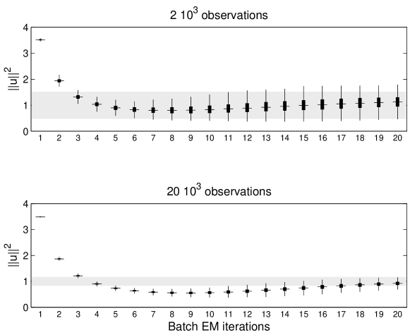
Figure 1: Convergence of batch EM estimates of $\|u\|^{2}$ as a function of the number of EM iterations for 2,000 (top) and 20,000 (bottom) observations. The box-and-whisker plots (outliers plotting suppressed) are computed from 1,000 independent replications of the simulated data. The grey region corresponds to $\pm 2$ interquartile range (approx. $99.3$% coverage) under the asymptotic Gaussian approximation of the MLE.

Figure 1 displays the results obtained with the batch EM algorithm for the single component PCA model estimated from data simulated under the model with $u$ being a 20-dimensional vector of unit norm and $\lambda=5$. Both $u$ and $\lambda$ are treated as unknown parameters but only the estimated squared norm of $u$ is displayed on Figure 1, as a function of the number of EM iterations and for two different data sizes. Note that in this very simple model, the observation likelihood being given the ${\operatorname{\mathcal{N}}}(0,uu^{\prime}+\lambda I_{d})$ density, it is straightforward to check that the Fisher information for the parameter $\|u\|^{2}$ equals $\{2(\lambda+\|u\|^{2})^{2}\}^{-1}$, which has been used to represent the asymptotic confidence interval in grey. The width of this interval is meant to be directly comparable to that of the whiskers in the box-and-whisker plots. Boxplots are used to summarise the results obtained from one thousand independent runs of the method.

Comparing the top and bottom plots clearly shows that when the number of iterations increases, the trajectories of the EM algorithm converge to a fixed deterministic trajectory which is that of the limiting EM recursion $(T^{k}_{\Theta}(\theta_{0}))_{k\geq 1}$. Of course, this trajectory depends on the choice of the initial point $\theta_{0}$ which was fixed throughout this experiment. It is also observed that the monotone increase in the likelihood guaranteed by the EM algorithm does not necessarily imply a monotone convergence of all parameters towards the MLE. Hence, if the number of EM iterations is kept fixed, the estimates returned by the batch EM algorithm with the larger number of observations (bottom plot) are not significantly improved despite the ten-fold increase in computation time (the E step computations must be done for all observations and hence the complexity of the E-step scales proportionally to the number $n$ of observations). From a statistical perspective, the situation is even less satisfying as estimation errors that were not statistically significant for 2,000 observations can become significant when the number of observations increases. In the upper plot, interrupting the EM algorithm after 3 or 4 iterations does produce estimates that are statistically acceptable (comparable to the exact MLE) but in the lower plot, about 20 iterations are needed to achieve the desired precision. As suggested by Neal and Hinton, (1999), this paradoxical situation can to some extent be avoided by updating the parameter (that is, applying the M-step) more often, without waiting for a complete scan of the data record.

3 Online Expectation-Maximisation

3.1 The Algorithm

The limiting-EM argument developed in the following section shows that when the number of observations tends to infinity, the EM algorithm is trying to locate the fixed points of the mapping $T_{\mathcal{S}}$ defined in (8), that is, the roots of the equation

$${\operatorname{E}}_{\pi}\left({\operatorname{E}}_{\bar{\theta}(S)}\left[\left.s(X_{1},Y_{1})\right|Y_{1}\right]\right)-S=0\,.$$ (10)

Although we cannot compute the required expectation wrt. the unknown distribution $\pi$ of the data, each new observation provides us with an unbiased noisy observation of this quantity through ${\operatorname{E}}_{\bar{\theta}(S)}\left[\left.s(X_{n},Y_{n})\right|Y_{n}\right]$. Solving (10) is thus an instance of the most basic case where the Stochastic Approximation (or Robbins-Monro) method can be used. The literature on Stochastic Approximation is huge but we recommend the textbooks by Benveniste et al., (1990), Kushner and Yin, (2003) for more details and examples as well as the review paper by Lai, (2003) for a historical perspective. The standard stochastic approximation approach to approximate the solution of (10) is to compute

$$S_{n}=S_{n-1}+\gamma_{n}\left({\operatorname{E}}_{\bar{\theta}(S_{n-1})}\left[\left.s(X_{n},Y_{n})\right|Y_{n}\right]-S_{n-1}\right)\,,$$ (11)

for $n\geq 1$, $S_{0}$ being arbitrary and $(\gamma_{n})_{n\geq 1}$ denoting a sequence of positive stepsizes that decrease to zero. This equation, rewritten in an equivalent form below, is the main ingredient of the online EM algorithm.

Algorithm 4 (Online EM Algorithm).

Given $S_{0},\theta_{0}$ and a sequence of stepsizes $(\gamma_{n})_{n\geq 1}$, do, for $n\geq 1$,

Stochastic E-Step

$$S_{n}=(1-\gamma_{n})S_{n-1}+\gamma_{n}{\operatorname{E}}_{\theta_{n-1}}\left[\left.s(X_{n},Y_{n})\right|Y_{n}\right]\,,$$ (12)

M-Step

$$\theta_{n}=\bar{\theta}(S_{n})\,.$$ (13)

Rewriting (10) under the form displayed in (12) is very enlightening as it shows that the new statistic $S_{n}$ is obtained as a convex combination of the previous statistic $S_{n-1}$ and of an update that depends on the new observation $Y_{n}$. In particular it shows that the stepsizes $\gamma_{n}$ have a natural scale as their highest admissible value is equal to one. This means that one can safely take $\gamma_{1}=1$ and that only the rate at which the stepsize decreases needs to be selected carefully (see below). It is also observed that if $\gamma_{1}$ is set to one, the initial value of $S_{0}$ is never used and it suffices to select the initial parameter guess $\theta_{0}$; this is the approach used in the following simulations.

The only adjustment to Algorithm 4 that is necessary in practice is to omit the M-step of (13) for the first observations. It typically takes a few observations before the complete-data maximum likelihood solution is well-defined and the parameter update should be inhibited during this early phase of training (Cappé and Moulines,, 2009). In the simulations presented below in Sections 3.2 and 3.4, the M-step was omitted for the first five observations only but in most complex scenarios a longer initial parameter freezing phase may be necessary.

When $\gamma_{1}<1$, it is tempting to interpret the value of $S_{0}$ as being associated to a prior on the parameters. Indeed, the choice of a conjugate prior for $\theta$ in the exponential family defined by (1) does result in a complete-data Maximum A Posteriori (MAP) estimate of $\bar{\theta}$ given by $\bar{\theta}(S_{n,k}+S_{0}/n)$ (instead of $\bar{\theta}(S_{n,k})$ for the MLE), where $S_{0}$ is the hyper-parameter of the prior (Robert,, 2001). However, it is easily checked that the influence of $S_{0}$ in $S_{n}$ decreases as $\prod_{k=1}^{n}(1-\gamma_{k})$, which for the suitable stepsize decrease schemes (see beginning of Section 3.2 below), decreases faster than $1/n$. Hence, the value of $S_{0}$ has a rather limited impact on the convergence of the online EM algorithm. To achieve MAP estimation (assuming a conjugate prior on $\theta$) it is thus recommend to replace (13) by $\theta_{n}=\bar{\theta}(S_{n}+S_{0}/n)$, where $S_{0}$ is the hyperparameter of the prior on $\theta$.

A last remark of importance is that Algorithm 4 can most naturally be interpreted as a stochastic approximation recursion on the sufficient statistics rather than on the parameters. There does not exists a similar algorithm that operates directly on the parameters because unbiased approximations of the rhs. of (9) based on the observations $Y_{t}$ are not easily available. As we will see below, Algorithm 4 is asymptotically equivalent to a gradient recursion on $\theta_{n}$ that involves an additional matrix weighting which is not necessary in (12).

3.2 Convergence Properties

Under the assumption that the stepsize sequence satisfies $\sum_{n}\gamma_{n}=\infty$, $\sum_{n}\gamma_{n}^{2}<\infty$ and other regularity hypotheses that are omitted here (see Cappé and Moulines,, 2009 for details) the following properties characterise the asymptotic behaviour of the online EM algorithm.

1. The estimates $\theta_{n}$ converge to the set of roots of the equation $\nabla_{\theta}D(\pi|f_{\theta})=0$.

2. The algorithm is asymptotically equivalent to a gradient algorithm

   $$\theta_{n}=\theta_{n-1}+\gamma_{n}J^{-1}(\theta_{n-1})\nabla_{\theta}\log f_{\theta_{n-1}}(Y_{n})\,,$$ (14)

   where $J(\theta)=-{\operatorname{E}}_{\pi}\left({\operatorname{E}}_{\theta}\left[\nabla_{\theta}^{2}\log p_{\theta}(X_{1},Y_{1})\big{|}Y_{1}\right]\right)$.

3. For a well specified model (i.e., if $\pi=f_{\theta_{\star}}$) and under Polyak-Ruppert averaging, $\theta_{n}$ is Fisher efficient: sequences that do converge to $\theta_{\star}$ are such that $\sqrt{n}(\theta_{n}-\theta_{\star})$ converges in distribution to a centred multivariate Gaussian variable with covariance matrix $I_{\pi}(\theta_{\star})$, where $I_{\pi}(\theta)=-{\operatorname{E}}_{\pi}[\nabla^{2}_{\theta}\log f_{\theta}(Y_{1})]$ is the Fisher information matrix corresponding to the observed data.

Polyak-Ruppert averaging refers to a postprocessing step which simply consists in replacing the estimated parameter values $\theta_{n}$ produced by the algorithm by their average

$$\tilde{\theta}_{n}=\frac{1}{n-n_{0}}\sum_{t=n_{0}+1}^{n}\theta_{n}\,,$$

where $n_{0}$ is a positive index at which averaging is started (Polyak and Juditsky,, 1992, Ruppert,, 1988). Regarding the statements (i) and (ii) above, it is important to understand that the limiting estimating equation $\nabla_{\theta}D(\pi|f_{\theta})=0$ may have multiple solutions, even in well-specified models. In practice, the most important factor that influences the convergence to one of the stationary points of the Kullback-Leibler divergence $D(\pi|f_{\theta})$ rather than the other is the choice of the initial value $\theta_{0}$. An additional important remark about (i)–(iii) is the fact that the asymptotic equivalent gradient algorithm in (14) is not a practical algorithm as the matrix $J(\theta)$ depends on $\pi$ and hence cannot be computed. Note also that $J(\theta)$ is (in general) neither equal to the complete-data information matrix $I_{p}(\theta)$ nor to the actual Fisher information in the observed model $I_{\pi}(\theta)$. The form of $J(\theta)$ as well as its role to approximate the convergence behaviour of the EM algorithm follows the idea of Lange, (1995).

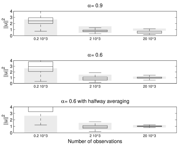
Figure 2: Online EM estimates of $\|u\|^{2}$ for various data sizes (200, 2,000 and 20,000 observations, from left to right) and algorithm settings ($\alpha=0.9$, $\alpha=0.6$ and $\alpha=0.6$ with Polyak-Ruppert averaging, from top to bottom). The box-and-whisker plots (outliers plotting suppressed) are computed from 1,000 independent replications of the simulated data. The grey regions corresponds to $\pm 2$ interquartile range (approx. $99.3$% coverage) under the asymptotic Gaussian approximation of the MLE.

From our experience, it is generally sufficient to consider stepsize sequences of the form $\gamma_{n}=1/n^{\alpha}$ where the useful range of values for $\alpha$ is from 0.6 to 0.9. The most robust setting is obtained when taking $\alpha$ close to $0.5$ and using Polyak-Ruppert averaging. The latter however requires to chose an index $n_{0}$ that is sufficiently large and, hence, some idea of the convergence time is necessary. To illustrate these observations, Figure 2 displays the results of online EM estimation for the single component PCA model, exactly in the same conditions as those considered previously for batch EM estimation in Section 2.3.

From a computational point of view, the main difference between the online EM algorithm and the batch EM algorithm of Section 2.1 is that the online algorithm performs the M-step update in (7) after each observation, according to (13), while the batch EM algorithm only applies the M-step update after a complete scan of all available observations. Both algorithms however require the computation of the E-step statistics following (6) for each observation. In batch EM, these local E-step computation are accumulated, following (4), while the online algorithm recursively averages these according to (12). Hence, as the computational complexity of the E and M steps are, in this case, comparable, the computational complexity of the online estimation is equivalent to that of one or two batch EM iterations. With this in mind, it is obvious that the results of Figure 2 compare very favourably to those of Figure 1 with an estimation performance that is compatible with the statistical uncertainty for observation lengths of 2,000 and larger (last two boxplots on the right in each display).

Regarding the choice of the stepsize decrease exponent $\alpha$, it is observed that while the choice of $\alpha=0.6$ (middle plot) does result in more variability than the choice of $\alpha=0.9$ (top plot), especially for smaller observation sizes, the long-run performance is somewhat better with the former. In particular, when Polyak-Ruppert averaging is used (bottom plot), the performance for the longest data size (20,000 observations) is clearly compatible with the claim that online EM is Fisher-efficient in this case. A practical concern associated with averaging is the choice of the initial instant $n_{0}$ where averaging starts. In the case of Figure 2, we choose $n_{0}$ to be equal to half the length of each data record, hence averaging is used only on the second half of the data. While it produces refined estimates for the longer data sizes, one can observe that the performance is rather degraded for the smallest observation size (200 observations) due to the fact that the algorithm is still very far from having converged after just 100 observations. Hence, averaging is efficient but does require to chose a value of $n_{0}$ that is sufficiently large so as to avoid introducing a bias due to the lack of convergence.

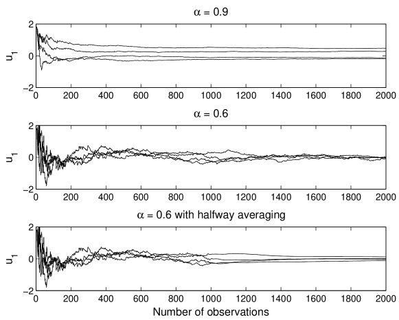
Figure 3: Four superimposed trajectories of the estimate of $u_{1}$ (first component of $u$) for various algorithm settings ($\alpha=0.9$, $\alpha=0.6$ and $\alpha=0.6$ with Polyak-Ruppert averaging, from top to bottom). The actual value of $u_{1}$ is equal to zero.

In our experience, the fact that choices of $\alpha$ close to 0.5 are more reliable than values closer to the upper limit of 1 is a very constant observation. It may come to some surprise for readers familiar with the gradient descent algorithm as used in numerical optimisation, which shares some similarity with (12). In this case, it is known that the optimal stepsize choice is of the form $\gamma_{n}=a(n+b)^{-1}$ for a broad class of functions (Nesterov,, 2003). However, the situation here is very different as we do not observe exact gradient or expectations but only noisy version of them. Figure 3 shows that while the trajectory of the parameter estimates appears to be much rougher and variable with $\alpha=0.6$ than with $\alpha=0.9$, the bias caused by the initialisation is also forgotten much more rapidly. It is also observed that the use of averaging (bottom display) makes it possible to achieve the best of both worlds (rapid forgetting of the initial condition and smooth trajectories).

Liang and Klein, (2009) considered the performance of the online EM algorithm for large-scale natural language processing applications. This domain of application is characterised by the use of very large-dimensional models, most often related to the multinomial distribution, involving tens of thousands of different words and tens to hundreds of semantic tags. As a consequence, each observation, be it a sentence or a whole document, is poorly informative about the model parameters (typically a given text contains only a very limited portion of the whole available vocabulary). In this context, Liang and Klein, (2009) found that the algorithm was highly competitive with other approaches but only when combined with mini-batch blocking: rather than applying Algorithm 4 at the observation scale, the algorithm is used on mini-batches consisting of $m$ consecutive observations $(Y_{m(k-1)+1},Y_{mk+2}\dots,Y_{mk})_{k\geq 1}$. For the models and data considered by Liang and Klein, (2009), values of $m$ of up to a few thousands yielded optimal performance. More generally, mini-batch blocking can be useful in dealing with mixture-like models with rarely active components.

3.3 Application to Finite Mixtures

Although we considered so far only the simple case of Example 2 which allows for the computation of the Fisher information matrix and hence for quantitative assessment of the asymptotic performance, the online EM algorithm is easy to implement in models involving finite mixture of distributions.

Figure 4 displays the Bayesian network representation corresponding to a mixture model: for each observation $Y_{t}$ there is an unobservable mixture indicator or allocation variable $X_{t}$ that takes its value in the set $\{1,\dots,m\}$. A typical parameterisation for this model is to have a separate sets of parameters $\omega$ and $\beta$ for, respectively, the parameters of the prior on $X_{t}$ and of the conditional distribution of $Y_{t}$ given $X_{t}$. Usually, $\omega=(\omega^{(1)},\dots,\omega^{(m)})$ is chosen to be the collection of component frequencies, $\omega^{(i)}={\operatorname{P}}_{\theta}(X_{t}=i)$, and hence $\omega$ is constrained to the probability simplex ($\omega^{(i)}\geq 0$ and $\sum_{i=1}^{m}\omega^{(i)}=1$). The observation pdf is most often parameterised as

$$f_{\theta}(y_{t})=\sum_{i=1}^{m}\omega^{(i)}g_{\beta^{(i)}}(y_{t})\,,$$

where $(g_{\lambda})_{\lambda\in\Lambda}$ is a parametric family of probability densities and $\beta=(\beta^{(1)},\dots,\beta^{(m)})$ are the component-specific parameters. We assume that $g_{\lambda}(y_{t})$ has an exponential family representation similar to that of (1) with sufficient statistic $s(y_{t})$ and maximum likelihood function $\bar{\lambda}:\mathcal{S}\mapsto\Lambda$, which is such that $\bar{\lambda}(\frac{1}{n}\sum_{t=1}^{n}s(Y_{t}))=\arg\max_{\lambda\in\Lambda}\frac{1}{n}\sum_{t=1}^{n}\log g_{\lambda}(Y_{t})$. It is then easily checked that the complete-data likelihood $p_{\theta}$ belongs to an exponential family with sufficient statistics

$$s^{(\omega,i)}(X_{t})={\mathbbm{1}}\{X_{t}=i\}\,,$$

$$s^{(\beta,i)}(X_{t},Y_{t})={\mathbbm{1}}\{X_{t}=i\}s(Y_{t})\,,\quad\text{for $i=1,\dots,m$.}$$

And the function $\bar{\theta}(S)$ can then be decomposed as

$$\omega^{(i)}=S^{(\omega,i)}\,,$$

$$\beta^{(i)}=\bar{\lambda}\left(S^{(\lambda,i)}/S^{(\omega,i)}\right)\,,\quad\text{for $i=1,\dots,m$.}.$$

Hence the online EM algorithm takes the following specific form.

Figure 4: Bayesian network representation of a mixture model.

Algorithm 5 (Online EM Algorithm for Finite Mixtures).

Given $S_{0},\theta_{0}$ and a sequence of stepsizes $(\gamma_{n})_{n\geq 1}$, do, for $n\geq 1$,

Stochastic E-Step

Compute

$$P_{\theta_{n-1}}(X_{t}=i|Y_{t})=\frac{\omega_{n-1}^{(i)}\,g_{\beta_{n-1}^{(i)}}(Y_{t})}{\sum_{j=1}^{m}\omega_{n-1}^{(j)}\,g_{\beta_{n-1}^{(j)}}(Y_{t})}\,,$$

and

$$S_{n}^{(\omega,i)}=(1-\gamma_{n})S_{n-1}^{(\omega,i)}+\gamma_{n}P_{\theta_{n-1}}(X_{t}=i|Y_{t})\,,$$

$$S_{n}^{(\beta,i)}=(1-\gamma_{n})S_{n-1}^{(\beta,i)}+\gamma_{n}s(Y_{t})P_{\theta_{n-1}}(X_{t}=i|Y_{t})\,,$$ (15)

for $i=1,\dots,m$.

M-Step

$$\omega_{n}^{(i)}=S_{n}^{(\omega,i)}\,,$$

$$\beta_{n}^{(i)}=\bar{\lambda}\left(S^{(\lambda,i)}_{n}/S^{(\omega,i)}_{n}\right)\,.$$ (16)

Example 6 (Online EM for Mixtures of Poisson).

We consider a simplistic instance of Algorithm 5 corresponding to the mixture of Poisson distribution (see also Section 2.4 of Cappé and Moulines,, 2009). In the case of the Poisson distribution, $g_{\lambda}(y_{t})=\frac{1}{y_{t}!}{\mathrm{e}}^{-\lambda}\lambda^{y}_{t}$, the sufficient statistic reduces to $s(y_{t})=y_{t}$ and the MLE function $\bar{\lambda}$ also is the identity $\bar{\lambda}(S)=S$. Hence, the online EM recursion for this case simply consists in instantiating (15)–(16) as

$$S_{n}^{(\omega,i)}=(1-\gamma_{n})S_{n-1}^{(\omega,i)}+\gamma_{n}P_{\theta_{n-1}}(X_{t}=i|Y_{t})\,,$$

$$S_{n}^{(\beta,i)}=(1-\gamma_{n})S_{n-1}^{(\beta,i)}+\gamma_{n}Y_{t}P_{\theta_{n-1}}(X_{t}=i|Y_{t})\,,$$

and

$$\omega_{n}^{(i)}=S_{n}^{(\omega,i)}\,,$$

$$\beta_{n}^{(i)}=S^{(\lambda,i)}_{n}/S^{(\omega,i)}_{n}\,.$$

3.4 Use for Batch Maximum-Likelihood Estimation

An interesting issue that deserves some more comments is the use of the online EM algorithm for batch estimation from a fixed data record $Y_{1},\dots,Y_{N}$. In this case, the objective is to save on computational effort compared to the use of the batch EM algorithm.

The analysis of the convergence behaviour of online EM in this context is made easy by the following observation: Properties (i) and (ii) stated at the beginning of Section 3.2 do not rely on the assumption that the model is well-specified (i.e., that $\pi=f_{\theta_{\star}}$) and can thus be applied with $\pi$ being the empirical distribution $\hat{\pi}_{N}(dy)=\frac{1}{N}\sum_{t=1}^{N}\delta_{Y_{t}}(dy)$ associated to the observed sample. Hence, if the online EM algorithm is applied by randomly drawing (with replacement) subsequent “pseudo-observations” from the finite set $\{Y_{1},\dots,Y_{N}\}$, it converges to points such that

$$\nabla_{\theta}D(\hat{\pi}_{N}|f_{\theta})=-\frac{1}{N}\nabla_{\theta}\sum_{t=1}^{N}\log f_{\theta}(Y_{t})=0\,,$$

that is, stationary points of the log-likelihood of the observations $Y_{1},\dots,Y_{N}$. Property (ii) also provides an asymptotic equivalent of the online EM update, where the index $n$ in (14) should be understood as the number of online EM steps rather than the number of actual observation, which is here fixed to $N$.

In practice, it doesn’t appear that drawing randomly the pseudo-observations make any real difference when the observations $Y_{1},\dots,Y_{N}$ are themselves already independent, except for very short data records. Hence, it is more convenient to scan the observation systematically in tours of length $N$ in which each observation is visited in a predetermined order. At the end of each tour, $k=n/N$ is equal to the number of batch tours completed since the start of the online EM algorithm.

To compare the numerical efficiency of this approach with that of the usual batch EM it is interesting to bring together two results. For online EM, based on (14), it is possible to show that $\sqrt{n}(\theta_{n}-\theta_{\infty})$ converges in distribution to a multivariate Gaussian distribution, where $\theta_{\infty}$ denotes the limit of $\theta_{n}$. In contrast, the batch EM algorithm achieves so-called linear convergence which means that for sufficiently large $k$’s, there exists $\rho<1$ such that $\|\theta_{k}-\theta_{\infty}\|\leq\rho^{k}$, where $\theta_{k}$ denotes the parameter estimated after $k$ batch EM iterations (Dempster et al.,, 1977, Lange,, 1995). In terms of computing effort, the number $k$ of batch EM iterations is comparable to the number $k=n/N$ of batch tours in the online EM algorithm. Hence the previous theoretical results suggest that

• If the number of available observations $N$ is small, batch EM can be way faster than the online EM algorithm, especially if one wants to obtain a very accurate numerical approximation of the MLE. Note that from a statistical viewpoint, this may be unnecessary as the MLE itself is only a proxy for the actual parameter value, with an error that is of order $1/\sqrt{N}$ in regular statistical models.

• When $N$ increases, the online EM algorithm becomes preferable and, indeed, arbitrary so if $N$ is sufficient large. Recall in particular from Section 3.2 that when $N$ increases, the online EM estimate obtained after a single batch tour is asymptotically equivalent to the MLE whereas the estimate obtained after a single batch EM iteration converges to the deterministic limit $T_{\Theta}(\theta_{0})$.

In their pioneering work on this topic, Neal and Hinton, (1999) suggested an algorithm called incremental EM as an alternative to the batch EM algorithm. The incremental EM algorithm turns out to be exactly equivalent to Algorithm 4 used with $\gamma_{n}=1/n$ up to the end of the batch tour only. After this initial batch scan, the incremental EM proceeds a bit differently by replacing one by one the previously computed values of ${\operatorname{E}}_{\theta_{t-1}}\left[\left.s(X_{t},Y_{t})\right|Y_{t}\right]$ with ${\operatorname{E}}_{\theta_{t-1}+(k-1)N}\left[\left.s(X_{t},Y_{t})\right|Y_{t}\right]$ when processing the observation at position $t$ for the $k$-th time. This incremental EM algorithm is indeed more efficient than batch EM, although they do not necessarily have the same complexity —a point that will be further discussed in the next section. For large values of $N$ however, incremental EM becomes impractical (due to the use of a storage space that increases proportionally to $N$) and less recommendable than the online EM algorithm as shown by the following example (see also the experiments of Liang and Klein,, 2009 for similar conclusions).

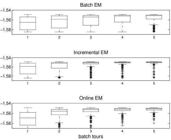
Figure 5: Normalised log-likelihood of the estimates obtained with, from top to bottom, batch EM, incremental EM and online EM as a function of the number of batch tours (or iterations, for batch EM). The data is of length $N=100$ and the box an whiskers plots summarise the results of 500 independent runs of the algorithms started from randomised starting points $\theta_{0}$.

Figure 6: Same display as in Figure 5 for a data record of length $N=\text{1,000}$.

Figure 5 displays the normalised log-likelihood values corresponding to the three estimation algorithms (batch EM, incremental EM and online EM) used to estimate the parameters of a mixture of two Poisson distributions (see Example 6 for implementation details). All data is simulated from a mixture model with parameters $\omega^{(1)}=0.8$, $\beta^{(1)}=1$ and $\beta^{(2)}=3$. In this setting, where the sample size is fixed, it is more difficult to come up with a faithful illustration of the merits of each approach as the convergence behaviour of the algorithms depend very much on the data record and on the initialisation. In Figures 5 and 6, the two data sets were kept fixed throughout the simulations but the initialisation of both Poisson means was randomly chosen from the interval [0.5,5]. This randomisation avoids focussing on particular algorithm trajectories and gives a good idea of the general situation, although some variations can still be observed when varying the observation records.

Figure 5 corresponds to the case of an observation sequence of length $N=100$. In this case it is observed that the performance of incremental EM dominates that of the other two algorithms, while the online EM algorithm only becomes preferable to batch EM after the second batch tour. For the data record of length $N=\text{1,000}$ (Figure 6), online EM now dominates the other two algorithms, with incremental still being preferable to batch EM. Notice that it is also the case after the first batch tour, illustrating our claim that the choice of $\gamma_{n}=n^{-0.6}$ used here for the online EM algorithm is indeed preferable to the value of $\gamma_{n}=n^{-1}$, which coincides with the update used by the incremental EM algorithm during the first batch tour. Finally, one can observe on Figure 6 that even after five EM iterations there are a few starting values for which batch EM or incremental EM gets stuck in regions of low normalised log-likelihood (around -1.6). These indeed correspond to local maxima of the log-likelihood and some trajectories of batch EM converge to these regions, depending on the value of initialisation. The online EM with the above choice of step-size appears to be less affected by this issue, although we have seen that in general only convergence to a stationary point of the log-likelihood is guaranteed.

4 Discussion

We conclude this chapter by a discussion of the online EM algorithm.

First, the approach presented here is not the only option for online parameter estimation in latent variable models. One of the earliest and most widely used (see, e.g., Liu et al.,, 2006) algorithm is that of Titterington, (1984) consisting of the following gradient update:

$$\theta_{n}=\theta_{n-1}+\gamma_{n}I^{-1}_{p}(\theta_{n-1})\nabla_{\theta}\log f_{\theta_{n-1}}(Y_{n})\,,$$ (17)

where the matrix $I_{p}$ refers to the complete-data Fisher information matrix. For complete-data models in natural parameterisation —with $\psi\equiv 1$ in (1), $I_{p}(\theta)$ coincides with $\nabla_{\theta}^{2}A(\theta)$ and, as it does not depend on $X_{t}$ or $Y_{t}$, is also equal to the matrix $J(\theta)$ that appears in (14). Thus, Titterington’s algorithm is in this case asymptotically equivalent to online EM. In other cases, where $I_{p}$ and $J$ differs, the recursion of (17) converges at the same rate as the online EM algorithm but is not Fisher-efficient. Another difference is the way Algorithm 4 deals with parameter constraints. Assumption 1 implies that the M-step update, taking into account the possible parameter constraints, is explicit. Hence, $\theta_{n}=\bar{\theta}(S_{n})$ does satisfy the parameter constraint by definition of the function $\bar{\theta}$. In the case of Example 6 for instance, the proposed update does guarantee that the mixture weight vector $\omega$ stays in the probability simplex. This is not the case with the update of (17) which requires reparameterisation or reprojection to handle possible parameter constraints.

As discussed in Section 3.4, the online EM algorithm is inspired by the work of Neal and Hinton, (1999) but distinct from their incremental EM approach. To the best of our knowledge, the online EM algorithm was first proposed by Sato, (2000) and Sato and Ishii, (2000) who described the algorithm and provided some analysis of convergence in the case of exponential families in natural parameterisation and for the case of mixtures of Gaussians.

In Section 3.4, we have seen that the online EM algorithm is preferable to batch EM, in terms of computational effort, when the observation size is sufficiently large. To operate in batch mode, the online EM needs to be used repeatedly by scanning the data record several times so as to converge toward the maximum likelihood estimate. It is important to note however that one iteration of batch EM operating on $N$ observations requires $N$ individual E-step computations but only one application of the M-step update; whereas online EM applies the M-step update at each observation and, hence, requires $N$ M-step updates per complete batch scan. Thus, the comparison between both approaches also depends on the respective numerical complexities of the E and M steps. The online approach is more attractive for models in which the M-step update is relatively simple. The availability of parallel computing resources would be most favourable to batch EM for which the E-step computations pertaining to each observation may be done independently. In contrast, in the online approach the computations are necessarily sequential as the parameter is updated when processing each observation.

As indicated in the beginning of this chapter, the main strength of the online EM algorithm is its simplicity and ease of implementation. As discussed above, this is particularly true in the presence of constraints on the parameter values. We have also seen in Section 3.2, that Algorithm 4 is very robust with respect to the choice of the stepsize $\gamma_{n}$. In particular, the absolute scale of the stepsize is fixed due to the use of a convex combination in (12) and it is generally sufficient to consider stepsizes of the form $\gamma_{n}=n^{-\alpha}$. We have shown that values of $\alpha$ of the order of 0.6 (i.e., closer to the lower limit of 0.5 than to the upper one of 1) yield more robust convergence. In addition, Polyak-Ruppert averaging can be used to smooth the parameter estimates and reach the optimal asymptotic rate of convergence that makes the online estimate equivalent to the actual MLE.

As illustrated by Figure 2, the online EM algorithm is not optimal for short data records of, say, less than 100 to 1,000 observations and in this case performing batch mode estimation by repeatedly scanning the data is recommended (see Figure 5 for the typical improvement to expect from this procedure). The main limitation of the online EM algorithm is to require that the M-step update $\bar{\theta}$ be available in closed-form. In particular, it would be interesting to extend the approach to cases where $\bar{\theta}$ needs to be determined numerically, thus making it possible to handle mixtures of Generalised Linear Models for instance (and not only mixtures of linear regressions as in Cappé and Moulines,, 2009).

We finally mention two more directions in which recent works have proposed to extend the online EM framework. The first one concerns the case of non-independent observations and, in particular, of observations that follows a Hidden Markov Model (HMM) with Markov dependencies between successive states. Mongillo and Denève, (2008) and Cappé, (2009) have proposed an algorithm for HMMs that appears to be very reminiscent of Algorithm 4, although not directly interpretable as a stochastic approximation recursion on the expected sufficient statistics. The other topic of importance is motivated by the many cases where the E-step computation of ${\operatorname{E}}_{\theta_{n-1}}\left[\left.s(X_{n},Y_{n})\right|Y_{n}\right]$ is not feasible. This typically occurs when the hidden variable $X_{n}$ is a continuous variable. For such cases, a promising solution consists in approximating the E-step using some form of Monte Carlo simulations (see, e.g., Cappé,, 2009, Del Moral et al.,, 2009 for methods that use sequential Monte Carlo approaches). However much conceptual and theoretical work remains to be done, as the consistency result summarised in Section 3.2 only extends straightforwardly to the —rather limited— case of independent Monte Carlo draws $X_{n}^{(\theta_{n-1})}$ from the conditionals $p_{\theta_{n-1}}(x_{n}|Y_{n})$. In that case, $s(X_{n}^{(\theta_{n-1})},Y_{n})$ still provides an unbiased estimate of the limiting EM mapping in $\theta_{n-1}$ and the theory is very similar. In the more general case where Markov chain or sequential Monte Carlo simulations are used to produce the draws $X_{n}^{(\theta_{n-1})}$, the convergence of the online estimation procedure needs to be investigated with care.

References

- Benveniste et al., (1990) Benveniste, A., Métivier, M., and Priouret, P. (1990). Adaptive Algorithms and Stochastic Approximations, volume 22. Springer, Berlin. Translated from the French by Stephen S. S. Wilson.
- Bickel and Doksum, (2000) Bickel, P. J. and Doksum, K. A. (2000). Mathematical Statistics. Basic Ideas and Selected Topics. Prentice-Hall, 2nd edition.
- Cappé, (2009) Cappé, O. (2009). Online EM algorithm for hidden Markov models. Preprint.
- Cappé, (2009) Cappé, O. (2009). Online sequential Monte Carlo EM algorithm. In IEEE Workshop Statist. Signal Process. (SSP), Cardiff, Wales, UK.
- Cappé et al., (2006) Cappé, O., Charbit, M., and Moulines, E. (2006). Recursive EM algorithm with applications to DOA estimation. In Proc. IEEE Int. Conf. Acoust., Speech, Signal Process., Toulouse, France.
- Cappé et al., (2008) Cappé, O., Douc, R., Guillin, A., Marin, J.-M., and Robert, C. P. (2008). Adaptive importance sampling in general mixture classes. Statistics and Computing, 18(4):447–459.
- Cappé and Moulines, (2009) Cappé, O. and Moulines, E. (2009). On-line expectation-maximization algorithm for latent data models. J. Roy. Statist. Soc. B, 71(3):593–613.
- Césa-Bianchi and Lugosi, (2006) Césa-Bianchi, N. and Lugosi, G. (2006). Prediction, learning, and games. Cambridge Univ. Press.
- Chopin, (2002) Chopin, N. (2002). A sequential particle filter method for static models. Biometrika, 89:539–552.
- Del Moral et al., (2009) Del Moral, P., Doucet, A., and Singh, S. S. (2009). Forward smoothing using sequential Monte Carlo. Technical Report CUED/F-INFENG/TR 638, Cambridge University Engineering Department.
- Dempster et al., (1977) Dempster, A. P., Laird, N. M., and Rubin, D. B. (1977). Maximum likelihood from incomplete data via the EM algorithm. J. Roy. Statist. Soc. B, 39(1):1–38 (with discussion).
- Kantas et al., (2009) Kantas, N., Doucet, A., Singh, S., and Maciejowski, J. (2009). An overview of sequential Monte Carlo methods for parameter estimation in general state-space models. In Proc. IFAC Symposium on System Identification (SYSID).
- Kushner and Yin, (2003) Kushner, H. J. and Yin, G. G. (2003). Stochastic Approximation and Recursive Algorithms and Applications, volume 35. Springer, New York, 2nd edition.
- Lai, (2003) Lai, T. L. (2003). Stochastic approximation. Ann. Statist., 31(2):391–406.
- Lange, (1995) Lange, K. (1995). A gradient algorithm locally equivalent to the EM algorithm. J. Roy. Statist. Soc. B, 57(2):425–437.
- Lehmann and Casella, (1998) Lehmann, E. L. and Casella, G. (1998). Theory of Point Estimation. Springer, New-York, 2nd edition.
- Liang and Klein, (2009) Liang, P. and Klein, D. (2009). Online EM for unsupervised models. In Conference of the North American Chapter of the Association for Computational Linguistics (NAACL), pages 611–619, Boulder, Colorado. Association for Computational Linguistics.
- Liu et al., (2006) Liu, Z., Almhana, J., Choulakian, V., and McGorman, R. (2006). Online EM algorithm for mixture with application to internet traffic modeling. Comput. Statist. Data Anal., 50(4):1052–1071.
- Ljung and Söderström, (1983) Ljung, L. and Söderström, T. (1983). Theory and Practice of Recursive Identification. MIT Press.
- Meng and Van Dyk, (1997) Meng, X.-L. and Van Dyk, D. (1997). The EM algorithm — an old folk song sung to a fast new tune. J. Roy. Statist. Soc. B, 59(3):511–567.
- Mongillo and Denève, (2008) Mongillo, G. and Denève, S. (2008). Online learning with hidden Markov models. Neural Computation, 20(7):1706–1716.
- Neal and Hinton, (1999) Neal, R. M. and Hinton, G. E. (1999). A view of the EM algorithm that justifies incremental, sparse, and other variants. In Jordan, M. I., editor, Learning in graphical models, pages 355–368. MIT Press, Cambridge, MA, USA.
- Nesterov, (2003) Nesterov, Y. (2003). Introductory lectures on convex optimization: A basic course. Kluwer.
- Polyak and Juditsky, (1992) Polyak, B. T. and Juditsky, A. B. (1992). Acceleration of stochastic approximation by averaging. SIAM J. Control Optim., 30(4):838–855.
- Robert, (2001) Robert, C. P. (2001). The Bayesian Choice. Springer, New York, 2nd edition.
- Ruppert, (1988) Ruppert, D. (1988). Efficient estimation from a slowly convergent Robbins-Monro process. Technical Report 781, Cornell University, School of Operations Research and Industrial Engineering.
- Sato, (2000) Sato, M. (2000). Convergence of on-line EM algorithm. In prooceedings of the International Conference on Neural Information Processing, volume 1, pages 476–481.
- Sato and Ishii, (2000) Sato, M. and Ishii, S. (2000). On-line EM algorithm for the normalized Gaussian network. Neural Computation, 12:407–432.
- Slonim and Weiss, (2003) Slonim, N. and Weiss, Y. (2003). Maximum likelihood and the information bottleneck. In Advances in Neural Information Processing Systems (NIPS), volume 15, pages 335–342.
- Tipping and Bishop, (1999) Tipping, M. and Bishop, C. (1999). Probabilistic principal component analysis. J. Roy. Statist. Soc. B, 6(3):611–622.
- Titterington, (1984) Titterington, D. M. (1984). Recursive parameter estimation using incomplete data. J. Roy. Statist. Soc. B, 46(2):257–267.