Bidifferential calculus, matrix SIT
and sine-Gordon equations

Abstract

We express a matrix version of the self-induced transparency (SIT) equations in the bidifferential calculus framework. An infinite family of exact solutions is then obtained by application of a general result that generates exact solutions from solutions of a linear system of arbitrary matrix size. A side result is a solution formula for the sine-Gordon equation.

1. Introduction.

The bidifferential calculus approach (see [1] and the references therein) aims to extract the essence of integrability aspects of integrable partial differential or difference equations (PDDEs) and to express them, and relations between them, in a universal way, i.e. resolved from specific examples. A powerful, though simple to prove, result [1, 2, 3] (see section 6) generates families of exact solutions from a matrix linear system. In the following we briefly recall the basic framework and then apply the latter result to a matrix generalization of the SIT equations.

2. Bidifferential calculus.

A graded algebra is an associative algebra $\Omega$ over $\mathbb{C}$ with a direct sum decomposition $\Omega=\bigoplus_{r\geq 0}\Omega^{r}$ into a subalgebra $\mathcal{A}:=\Omega^{0}$ and $\mathcal{A}$-bimodules $\Omega^{r}$, such that $\Omega^{r}\,\Omega^{s}\subseteq\Omega^{r+s}$. A bidifferential calculus (or bidifferential graded algebra) is a unital graded algebra $\Omega$ equipped with two ($\mathbb{C}$-linear) graded derivations $\mathrm{d},\bar{\mathrm{d}}:\Omega\rightarrow\Omega$ of degree one (hence $\mathrm{d}\Omega^{r}\subseteq\Omega^{r+1}$, $\bar{\mathrm{d}}\Omega^{r}\subseteq\Omega^{r+1}$), with the properties

$$\mathrm{d}_{z}^{2}=0\qquad\forall z\in\mathbb{C}\,,\qquad\mbox{where}\quad\mathrm{d}_{z}:=\bar{\mathrm{d}}-z\,\mathrm{d}\,,$$ (1)

and the graded Leibniz rule $\mathrm{d}_{z}(\chi\,\chi^{\prime})=(\mathrm{d}_{z}\chi)\,\chi^{\prime}+(-1)^{r}\,\chi\,\mathrm{d}_{z}\chi^{\prime}$, for all $\chi\in\Omega^{r}$ and $\chi^{\prime}\in\Omega$.

3. Dressing a bidifferential calculus.

Let $(\Omega,\mathrm{d},\bar{\mathrm{d}})$ be a bidifferential calculus. Replacing $\mathrm{d}_{z}$ in (1) by $\mathrm{D}_{z}:=\bar{\mathrm{d}}-A-z\,\mathrm{d}$ with a 1-form $A\in\Omega^{1}$ (in the expression for $\mathrm{D}_{z}$ to be regarded as a multiplication operator), the resulting condition $\mathrm{D}_{z}^{2}=0$ (for all $z\in\mathbb{C}$) can be expressed as

$$\mathrm{d}A=0=\bar{\mathrm{d}}A-A\,A\;.$$ (2)

If (2) is equivalent to a PDDE, we have a bidifferential calculus formulation for it. This requires that $A$ depends on independent variables and the derivations $\mathrm{d},\bar{\mathrm{d}}$ involve differential or difference operators. Several ways exist to reduce the two equations (2) to a single one:
(1) We can solve the first of (2) by setting $A=\mathrm{d}\phi$. This converts the second of (2) into

$$\bar{\mathrm{d}}\,\mathrm{d}\,\phi=\mathrm{d}\phi\;\mathrm{d}\phi\;.$$ (3)

(2) The second of (2) can be solved by setting $A=(\bar{\mathrm{d}}g)\,g^{-1}$. The first equation then reads

$$\mathrm{d}\,\Big{(}(\bar{\mathrm{d}}g)\,g^{-1}\Big{)}=0\;.$$ (4)

(3) More generally, setting $A=[\bar{\mathrm{d}}g-(\mathrm{d}g)\Delta]\;g^{-1}$, with some $\Delta\in\mathcal{A}$, we have $\bar{\mathrm{d}}A-A\,A=(\mathrm{d}A)\,g\Delta g^{-1}+(\mathrm{d}g)\,(\bar{\mathrm{d}}\Delta-(\mathrm{d}\Delta)\,\Delta)\,g^{-1}$. As a consequence, if $\Delta$ is chosen such that $\bar{\mathrm{d}}\Delta=(\mathrm{d}\Delta)\,\Delta$, then the two equations (2) reduce to

$$\mathrm{d}\Big{(}[\bar{\mathrm{d}}g-(\mathrm{d}g)\Delta]\;g^{-1}\Big{)}=0\;.$$ (5)

With the choice of a suitable bidifferential calculus, (3) and (4), or more generally (5), have been shown to reproduce quite a number of integrable PDDEs. This includes the self-dual Yang-Mills equation, in which case (3) and (4) correspond to well-known potential forms [1]. Having found a bidifferential calculus in terms of which e.g. (3) is equivalent to a certain PDDE, it is not in general guaranteed that also (4) represents a decent PDDE. Then the generalization (5) has a chance to work (cf. [1]). In such a case, the Miura transformation

$$[\bar{\mathrm{d}}g-(\mathrm{d}g)\Delta]\;g^{-1}=\mathrm{d}\phi$$ (6)

is a hetero-Bäcklund transformation relating solutions of the two PDDEs.

Bäcklund, Darboux and binary Darboux transformations can be understood in this general framework [1], and there is a construction of an infinite set of (generalized) conservation laws. Exchanging $\mathrm{d}$ and $\bar{\mathrm{d}}$ leads to what is known in the literature as ‘negative flows’ [3].

4. A matrix generalization of SIT equations and its Miura-dual.

$\mathcal{A}=\mathrm{Mat}(n,n,C^{\infty}(\mathbb{R}^{2}))$ denotes the algebra of $n\times n$ matrices of smooth functions on $\mathbb{R}^{2}$. Let $\Omega=\mathcal{A}\otimes\bigwedge(\mathbb{C}^{2})$ with the exterior algebra $\bigwedge(\mathbb{C}^{2})$ of $\mathbb{C}^{2}$. In terms of coordinates $x,y$ of $\mathbb{R}^{2}$, a basis $\zeta_{1},\zeta_{2}$ of $\bigwedge^{1}(\mathbb{C}^{2})$, and a constant $n\times n$ matrix $J$, maps $\mathrm{d}$ and $\bar{\mathrm{d}}$ are defined as follows on $\mathcal{A}$,

$$\mathrm{d}f=\tfrac{1}{2}[J,f]\otimes\zeta_{1}+f_{y}\otimes\zeta_{2}\,,\qquad\bar{\mathrm{d}}f=f_{x}\otimes\zeta_{1}+\tfrac{1}{2}[J,f]\otimes\zeta_{2}$$

(see also [4]). They extend in an obvious way (with $\mathrm{d}\zeta_{i}=\bar{\mathrm{d}}\zeta_{i}=0$) to $\Omega$ such that $(\Omega,\mathrm{d},\bar{\mathrm{d}})$ becomes a bidifferential calculus. We find that (3) is equivalent to

$$\phi_{xy}=\tfrac{1}{2}\left[[J,\phi],\phi_{y}-\tfrac{1}{2}J\right]\;.$$ (7)

Let $n=2m$ and $J=\mbox{\rm block-diag}(I,-I)$, where $I=I_{m}$ denotes the $m\times m$ identity matrix. Decomposing $\phi$ into $m\times m$ blocks, and constraining it as follows,

$$\phi=\begin{pmatrix}p&q\\ q&-p\\ \end{pmatrix}\,,$$ (8)

(7) splits into the two equations

$$\begin{split}p_{xy}=(q^{2})_{y}\,,\qquad q_{xy}=q-p_{y}q-qp_{y}\;.\end{split}$$ (9)

We refer to them as matrix-SIT equations (see section 5), not purporting that they have a similar physical relevance as in the scalar case. The Miura transformation (6) (with $\Delta=0$) now reads

$$\begin{split}g_{x}\,g^{-1}=\tfrac{1}{2}\,[J,\phi]\,,\qquad\tfrac{1}{2}\,[J,g]\,g^{-1}=\phi_{y}\;.\end{split}$$ (10)

Writing

$$g=\begin{pmatrix}a&b\\ c&d\\ \end{pmatrix}\,,$$

with $m\times m$ matrices $a,b,c,d$, and assuming that $a$ and its Schur complement $\mathcal{S}(a)=d-c\,a^{-1}b$ is invertible (which implies that $g$ is invertible), (10) with (8) requires

$$b=-c\,a^{-1}d\,,\qquad a_{x}=-c_{x}\,a^{-1}c\,,\qquad d_{x}=-c_{x}\,a^{-1}c\,a^{-1}d\;.$$ (11)

The last equation can be replaced by $d_{x}\,d^{-1}=a_{x}\,a^{-1}$. Invertibility of $\mathcal{S}(a)$ implies that $d$ and $I+r^{2}$ are invertible, where $r:=c\,a^{-1}$. The conditions (11) are necessary in order that the Miura transformation relates solutions of (9) to solutions of its ‘dual’

$$(g_{x}\,g^{-1})_{y}=\tfrac{1}{4}\,[gJg^{-1},J]\,,$$ (12)

obtained from (4). Taking (11) into account, the Miura transformation reads

$$q=-c_{x}\,a^{-1}=-r_{x}-r\,a_{x}\,a^{-1}\,,\quad q_{y}=-r\,(I+r^{2})^{-1}\,,\quad p_{y}=I-(I+r^{2})^{-1}\;.$$ (13)

As a consequence, we have

$${q_{y}}^{2}+{p_{y}}^{2}=p_{y}\;.$$ (14)

Furthermore, the second of (11) and the first of (13) imply $a_{x}a^{-1}=qr$. Hence we obtain the system

$$r_{x}=-q-r\,q\,r\,,\qquad q_{y}=-r\,(I+r^{2})^{-1}\,,$$ (15)

which may be regarded as a matrix or ‘noncommutative’ generalization of the sine-Gordon equation. There are various such generalizations in the literature. The first equation has the solution $q=-\sum_{k=0}^{\infty}(-1)^{k}\,r^{k}\,r_{x}\,r^{k}$, if the sum exists. Alternatively, we can express this as $q=-(I+r_{L}r_{R})^{-1}(r_{x})$, where $r_{L}$ ($r_{R}$) denotes the map of left (right) multiplication by $r$. This can be used to eliminate $q$ from the second equation, resulting in

$$\left((I+r_{L}r_{R})^{-1}(r_{x})\right)_{y}=r\,(I+r^{2})^{-1}\;.$$ (16)

If $r=\tan(\theta/2)\,\boldsymbol{\pi}$ with a constant projection $\boldsymbol{\pi}$ (i.e. $\boldsymbol{\pi}^{2}=\boldsymbol{\pi}$) and a function $\theta$, then (16) reduces to the sine-Gordon equation

$$\theta_{xy}=\sin\theta\;.$$ (17)

(15) can be obtained directly from (12) as follows, by setting

$$g=\begin{pmatrix}a&-c\\ c&a\\ \end{pmatrix}=\begin{pmatrix}I&-r\\ r&I\\ \end{pmatrix}\,a\,,\quad\mbox{hence}\quad g^{-1}=a^{-1}\,\begin{pmatrix}I&r\\ -r&I\\ \end{pmatrix}\,(I+r^{2})^{-1}\;.$$

This leads to

$$\left((r_{x}\,r+r\rho\,r+\rho)(I+r^{2})^{-1}\right)_{y}=0\,,\quad\left((r_{x}+r\rho-\rho\,r)(I+r^{2})^{-1}\right)_{y}=r(I+r^{2})^{-1}\,,$$

where $\rho:=a_{x}a^{-1}$. Setting an integration ‘constant’ to zero, the first equation integrates to $\rho=-r_{x}r-r\rho\,r$. With its help, the second can be written as $(r_{x}+r\rho)_{y}=r(I+r^{2})^{-1}$. Since $q=-(ra)_{x}\,a^{-1}=-r_{x}-r\,\rho$, this is the second of (15). The first follows noting that $qr=\rho$.

5. Sharp line SIT equations and sine-Gordon.

We consider the scalar case, i.e. $m=1$. Introducing $\mathcal{E}=2\sqrt{\alpha}q$ with a positive constant $\alpha$, $\mathcal{P}=2q_{y}$, $\mathcal{N}=2p_{y}-1$, and new coordinates $z,t$ via $x=\sqrt{\alpha}(z-t)$ and $y=\sqrt{\alpha}z$, the system (9) is transformed into

$$\mathcal{P}_{t}=\mathcal{E}\,\mathcal{N}\,,\quad\mathcal{N}_{t}=-\mathcal{E}\,\mathcal{P}\,,$$

and the relation between $\mathcal{E}$ and $\mathcal{P}$ takes the form

$$\mathcal{E}_{z}+\mathcal{E}_{t}=\alpha\,\mathcal{P}\;.$$

These are the sharp line self-induced transparency (SIT) equations [5, 6, 7]. We note that $\mathcal{P}^{2}+\mathcal{N}^{2}$ is conserved. Indeed, as a consequence of (14), we have $\mathcal{P}^{2}+\mathcal{N}^{2}=1$. Writing $\mathcal{P}=-\sin\theta$ and $\mathcal{N}=-\cos\theta$, reduces the first two equations to $\mathcal{E}=\theta_{t}$. Expressed in the coordinates $x,y$, the third then becomes the sine-Gordon equation (17) (cf. [6]). As a consequence of the above relations, $q$ and $p$ depend as follows on $\theta$,

$$q=-\tfrac{1}{2}\theta_{x}\,,\qquad q_{y}=-\tfrac{1}{2}\sin\theta\,,\qquad p_{y}=\tfrac{1}{2}(1-\cos\theta)\;.$$ (18)

These are precisely the equations that result from the Miura transformation (10) (or from (13)), choosing

$$g=\begin{pmatrix}\cos{\tfrac{\theta}{2}}&-\sin{\tfrac{\theta}{2}}\\ \vskip 6.0pt plus 2.0pt minus 2.0pt\cr\sin{\tfrac{\theta}{2}}&\cos{\tfrac{\theta}{2}}\end{pmatrix}\,,$$

and (12) becomes the sine-Gordon equation (17). The conditions (11) are identically satisfied as a consequence of the form of $g$.

6. A universal method of generating solutions from a matrix linear system.

Theorem 1.

Let $(\Omega,\mathrm{d},\bar{\mathrm{d}})$ be a bidifferential calculus with $\Omega=\mathcal{A}\otimes\bigwedge(\mathbb{C}^{2})$, where $\mathcal{A}$ is the algebra of matrices with entries in some algebra $\mathcal{B}$ (where the product of two matrices is defined to be zero if the sizes of the two matrices do not match). For fixed $N,N^{\prime}$, let $\boldsymbol{X}\in\mathrm{Mat}(N,N,\mathcal{B})$ and $\boldsymbol{Y}\in\mathrm{Mat}(N^{\prime},N,\mathcal{B})$ be solutions of the linear equations

$$\bar{\mathrm{d}}\boldsymbol{X}=(\mathrm{d}\boldsymbol{X})\,\boldsymbol{P}\,,\qquad\bar{\mathrm{d}}\boldsymbol{Y}=(\mathrm{d}\boldsymbol{Y})\,\boldsymbol{P}\,,\qquad\boldsymbol{R}\,\boldsymbol{X}-\boldsymbol{X}\,\boldsymbol{P}=-\boldsymbol{Q}\,\boldsymbol{Y}\,,$$

with $\mathrm{d}$- and $\bar{\mathrm{d}}$-constant matrices $\boldsymbol{P},\boldsymbol{R}\in\mathrm{Mat}(N,N,\mathcal{B})$, and $\boldsymbol{Q}=\tilde{\boldsymbol{V}}\,\tilde{\boldsymbol{U}}$, where $\tilde{\boldsymbol{U}}\in\mathrm{Mat}(n,N^{\prime},\mathcal{B})$ and $\tilde{\boldsymbol{V}}\in\mathrm{Mat}(N,n,\mathcal{B})$ are $\mathrm{d}$- and $\bar{\mathrm{d}}$-constant. If $\boldsymbol{X}$ is invertible, the $n\times n$ matrix variable

$$\phi=\tilde{\boldsymbol{U}}\boldsymbol{Y}\boldsymbol{X}^{-1}\tilde{\boldsymbol{V}}\in\mathrm{Mat}(n,n,\mathcal{B})$$

solves $\bar{\mathrm{d}}\phi=(\mathrm{d}\phi)\,\phi+\mathrm{d}\vartheta$ with $\vartheta=\tilde{\boldsymbol{U}}\boldsymbol{Y}\boldsymbol{X}^{-1}\boldsymbol{R}\tilde{\boldsymbol{V}}$, hence (by application of $\mathrm{d}$) also (3). $\square$

There is a similar result for (5) [3]. The Miura transformation is a corresponding bridge.

7. Solutions of the matrix SIT equations.

From Theorem 1 we can deduce the following result, using straightforward calculations [8], analogous to those in [2] (see also [3]).

Proposition 2.

Let $\boldsymbol{S}\in\mathrm{Mat}(M,M,\mathbb{C})$ be invertible, $\boldsymbol{U}\in\mathrm{Mat}(m,M,\mathbb{C})$, $\boldsymbol{V}\in\mathrm{Mat}(M,m,\mathbb{C})$, and $\boldsymbol{K}\in\mathrm{Mat}(M,M,\mathbb{C})$ a solution of the Sylvester equation

$$\boldsymbol{S}\boldsymbol{K}+\boldsymbol{K}\boldsymbol{S}=\boldsymbol{V}\boldsymbol{U}\;.$$ (19)

Then, with $\boldsymbol{\Xi}=e^{-\boldsymbol{S}x-\boldsymbol{S}^{-1}y}$ and any $p_{0}\in\mathrm{Mat}(m,m,\mathbb{C})$ (more generally $x$-dependent),

$$\begin{split}q=\boldsymbol{U}\boldsymbol{\Xi}\,(\boldsymbol{I}_{M}+(\boldsymbol{K}\boldsymbol{\Xi})^{2})^{-1}\boldsymbol{V}\,,\qquad p=p_{0}-\boldsymbol{U}\boldsymbol{\Xi}\boldsymbol{K}\boldsymbol{\Xi}\,(\boldsymbol{I}_{M}+(\boldsymbol{K}\boldsymbol{\Xi})^{2})^{-1}\boldsymbol{V}\end{split}$$ (20)

(assuming the inverse exists) is a solution of (9). $\square$

If the matrix $\boldsymbol{S}$ satisfies the spectrum condition

$$\sigma(\boldsymbol{S})\cap\sigma(-\boldsymbol{S})=\emptyset$$ (21)

(where $\sigma(\boldsymbol{S})$ denotes the set of eigenvalues of $\boldsymbol{S}$), then the Sylvester equation (19) has a unique solution $\boldsymbol{K}$ (for any choice of the matrices $\boldsymbol{U},\boldsymbol{V}$), see e.g. [9].

By a lengthy calculation [8] one can verify directly that the solutions in Proposition 2 satisfy (14). Alternatively, one can show that these solutions actually determine solutions of the Miura transformation (cf. [3]), and we have seen that (14) is a consequence.

There is a certain redundancy in the matrix data that determine the solutions (20) of (9). This can be narrowed down by observing that the following transformations leave (19) and (20) invariant (see also the NLS case treated in [2]).
(1) Similarity transformation with an invertible $\boldsymbol{M}\in\mathrm{Mat}(M,M,\mathbb{C})$ :

$$\boldsymbol{S}\mapsto\boldsymbol{M}\boldsymbol{S}\boldsymbol{M}^{-1}\,,\quad\boldsymbol{K}\mapsto\boldsymbol{M}\boldsymbol{K}\boldsymbol{M}^{-1}\,,\quad\boldsymbol{V}\mapsto\boldsymbol{M}\boldsymbol{V}\,,\quad\boldsymbol{U}\mapsto\boldsymbol{U}\boldsymbol{M}^{-1}\;.$$

As a consequence, we can choose $\boldsymbol{S}$ in Jordan normal form without restriction of generality.
(2) Reparametrization transformation with invertible $\boldsymbol{A},\boldsymbol{B}\in\mathrm{Mat}(M,M,\mathbb{C})$ :

$$\boldsymbol{S}\mapsto\boldsymbol{S}\,,\quad\boldsymbol{K}\mapsto\boldsymbol{B}^{-1}\boldsymbol{K}\boldsymbol{A}^{-1}\,,\quad\boldsymbol{V}\mapsto\boldsymbol{B}^{-1}\boldsymbol{V}\,,\quad\boldsymbol{U}\mapsto\boldsymbol{U}\boldsymbol{A}^{-1}\,,\quad\boldsymbol{\Xi}\mapsto\boldsymbol{A}\boldsymbol{B}\boldsymbol{\Xi}\;.$$

(3) Reflexion symmetry:

$$\boldsymbol{S}\mapsto-\boldsymbol{S}\,,\quad\boldsymbol{K}\mapsto-\boldsymbol{K}^{-1}\,,\quad\boldsymbol{V}\mapsto\boldsymbol{K}^{-1}\boldsymbol{V}\,,\quad\boldsymbol{U}\mapsto\boldsymbol{U}\boldsymbol{K}^{-1}\,,\quad p_{0}\mapsto p_{0}-\boldsymbol{U}\boldsymbol{K}^{-1}\boldsymbol{V}\;.$$

This requires that $\boldsymbol{K}$ is invertible. More generally, such a reflexion can be applied to any Jordan block of $\boldsymbol{S}$ and then changes the sign of its eigenvalue [8] (see also [10, 2]). The Jordan normal form can be restored afterwards via a similarity transformation.

The following result is easily verified [8].

Proposition 3.

Let $\boldsymbol{S},\boldsymbol{U},\boldsymbol{V}$ be as in Proposition 2 and $\boldsymbol{T}\in\mathrm{Mat}(M,M,\mathbb{C})$ invertible.
(1) Let $\boldsymbol{T}$ be Hermitian (i.e. $\boldsymbol{T}^{\dagger}=\boldsymbol{T}$) and such that $\boldsymbol{S}^{\dagger}=\boldsymbol{T}\boldsymbol{S}\boldsymbol{T}^{-1}$, $\boldsymbol{U}=\boldsymbol{V}^{\dagger}\boldsymbol{T}$. Let $\boldsymbol{K}$ be a solution of (19), which can then be chosen such that $\boldsymbol{K}^{\dagger}=\boldsymbol{T}\boldsymbol{K}\boldsymbol{T}^{-1}$. Then $q$ and $p$ given by (20) with $p_{0}^{\dagger}=p_{0}$ are both Hermitian and thus solve the Hermitian reduction of (9).
(2) Let $\bar{\boldsymbol{T}}=\boldsymbol{T}^{-1}$ (where the bar means complex conjugation) and $\bar{\boldsymbol{S}}=\boldsymbol{T}\boldsymbol{S}\boldsymbol{T}^{-1}$, $\bar{\boldsymbol{U}}=\boldsymbol{U}\boldsymbol{T}^{-1}$ and $\bar{\boldsymbol{V}}=\boldsymbol{T}\boldsymbol{V}$. Let $\boldsymbol{K}$ be a solution of (19), which can then be chosen such that $\bar{\boldsymbol{K}}=\boldsymbol{T}\boldsymbol{K}\boldsymbol{T}^{-1}$. Then $q$ and $p$ given by (20) with $\bar{p}_{0}=p_{0}$ satisfy $\bar{q}=q$ and $\bar{p}=p$, and thus solve the complex conjugation reduction of (9). $\square$

8. Rank one solutions.

Let $M=1$. We write $\boldsymbol{S}=s$, $\boldsymbol{U}=\boldsymbol{u}$, $\boldsymbol{V}=\boldsymbol{v}^{\intercal}$, $\boldsymbol{K}=k$ (where ^⊺ means the transpose) and $\boldsymbol{\Xi}=\xi=e^{-sx-s^{-1}y}$. Then (19) yields $k=(\boldsymbol{v}^{\intercal}\boldsymbol{u})/(2s)$. From (20) we obtain

$$q=\frac{2\,s\,k\,\xi}{1+(k\xi)^{2}}\,\boldsymbol{\pi}\,,\quad p=\tilde{p}_{0}+\frac{2\,s}{1+(k\xi)^{2}}\,\boldsymbol{\pi}\,,\quad\tilde{p}_{0}:=p_{0}-2s\,\boldsymbol{\pi}\,,\quad\boldsymbol{\pi}:=\frac{\boldsymbol{u}\boldsymbol{v}^{\intercal}}{\boldsymbol{v}^{\intercal}\boldsymbol{u}}\;.$$

The Miura transformation (13) implies $r=-q_{y}\,(I-p_{y})^{-1}$, and we obtain

$$r=-\frac{2\,k\xi}{1-(k\xi)^{2}}\,\boldsymbol{\pi}\,,$$

which is singular. But $\theta=-2\arctan(2k\xi/[1-(k\xi)^{2}])$ is the single kink solution of the sine-Gordon equation (17).

9. Solutions of the scalar (sharp line) SIT equations.

We rewrite $p$ in (20), where now $m=1$, as follows,

$$p =p_{0}-\mathrm{tr}\left((\boldsymbol{S}\boldsymbol{K}+\boldsymbol{K}\boldsymbol{S})\,\boldsymbol{\Xi}\boldsymbol{K}\boldsymbol{\Xi}\,(\boldsymbol{I}_{M}+(\boldsymbol{K}\boldsymbol{\Xi})^{2})^{-1}\right)$$

$$=p_{0}+\mathrm{tr}\left((\boldsymbol{I}_{M}+(\boldsymbol{K}\boldsymbol{\Xi})^{2})_{x}\,(\boldsymbol{I}_{M}+(\boldsymbol{K}\boldsymbol{\Xi})^{2})^{-1}\right)$$

$$=p_{0}+\left(\log\det\left(\boldsymbol{I}_{M}+(\boldsymbol{K}\boldsymbol{\Xi})^{2}\right)\right)_{x}\,,$$ (22)

using (19) and the identity $(\det\boldsymbol{M})_{x}=\mathrm{tr}(\boldsymbol{M}_{x}\boldsymbol{M}^{-1})\,\det\boldsymbol{M}$ for an invertible matrix function $\boldsymbol{M}$. $q$ in (20) can be expressed as

$$q=2\,\mathrm{tr}\left(\boldsymbol{S}\boldsymbol{K}\boldsymbol{\Xi}\,(\boldsymbol{I}_{M}+(\boldsymbol{K}\boldsymbol{\Xi})^{2})^{-1}\right)\;.$$

In particular, if $\boldsymbol{S}$ is diagonal with eigenvalues $s_{i}$, $i=1,\ldots,M$, and satisfies (21), then the solution $\boldsymbol{K}$ of the Sylvester equation (19), which now amounts to $\mathrm{rank}(\boldsymbol{S}\boldsymbol{K}+\boldsymbol{K}\boldsymbol{S})=1$, is the Cauchy-type matrix with components $K_{ij}=v_{i}\,u_{j}/(s_{i}+s_{j})$, where $u_{i},v_{i}\in\mathbb{C}$. Figs. 1 and 2 show plots of two examples from the above family of solutions.

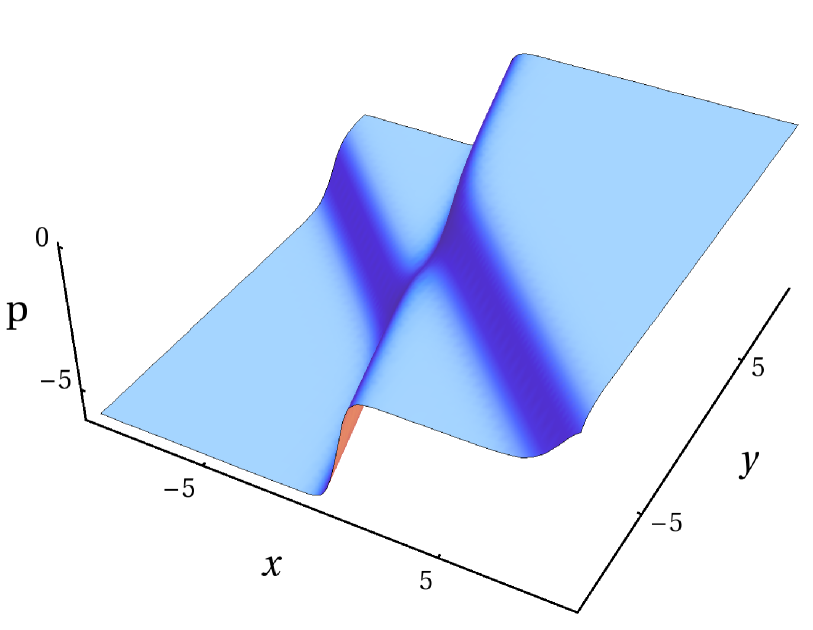
Figure 1: A scalar 2-soliton solution with $\boldsymbol{S}=\mathrm{diag}(1,2)$ and $u_{i}=v_{i}=1$.

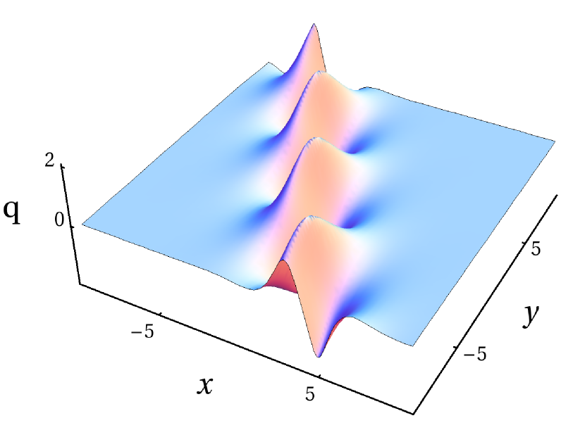
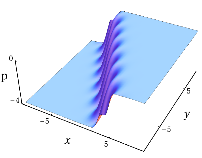
Figure 2: A scalar breather solution with $\boldsymbol{S}=\mathrm{diag}(1+\mathrm{i},1-\mathrm{i})$ and $u_{i}=v_{i}=1$.

10. A family of solutions of the real sine-Gordon equation.

Via the Miura transformation (18), Proposition 2 determines a family of sine-Gordon solutions (see also e.g. [6, 11, 12, 13, 14, 15, 16] for related results obtained by different methods).

Proposition 4.

Let $\boldsymbol{S}\in\mathrm{Mat}(M,M,\mathbb{C})$ be invertible and $\boldsymbol{K}\in\mathrm{Mat}(M,M,\mathbb{C})$ such that $\mathrm{rank}(\boldsymbol{S}\boldsymbol{K}+\boldsymbol{K}\boldsymbol{S})=1$, $\det(\boldsymbol{I}_{M}+(\boldsymbol{K}\boldsymbol{\Xi})^{2})\in\mathbb{R}$ with $\boldsymbol{\Xi}=e^{-\boldsymbol{S}x-\boldsymbol{S}^{-1}y}$, and $\mathrm{tr}(\boldsymbol{S}\boldsymbol{K}\boldsymbol{\Xi}\,(\boldsymbol{I}_{M}+(\boldsymbol{K}\boldsymbol{\Xi})^{2})^{-1})\not\in\mathrm{i}\mathbb{R}$ (where $\mathrm{i}$ is the imaginary unit). Then

$$\theta=4\arctan\Big{(}\frac{\sqrt{\beta}}{1+\sqrt{1-\beta}}\Big{)}\quad\mbox{with}\quad\beta:=\left(\log|\det(\boldsymbol{I}_{M}+(\boldsymbol{K}\boldsymbol{\Xi})^{2})|\right)_{xy}$$ (23)

solves the sine-Gordon equation $\theta_{xy}=\sin\theta$ in any open set of $\mathbb{R}^{2}$ where $\det(\boldsymbol{I}_{M}+(\boldsymbol{K}\boldsymbol{\Xi})^{2})\neq 0$.

Proof: Let $p$ be given by (22). Due to the assumption $\det(\boldsymbol{I}_{M}+(\boldsymbol{K}\boldsymbol{\Xi})^{2})\in\mathbb{R}$, $p_{y}$ is real, hence (14) implies $|1-2p_{y}|^{2}=1-4{q_{y}}^{2}$. It follows that ${q_{y}}^{2}$ is real. Since another of our assumptions excludes that $q_{y}$ is imaginary, it follows that $|1-2p_{y}|\leq 1$. Hence the equation $\cos\theta=1-2p_{y}$ (second of (18)) has a real solution $\theta$. Inserting the expression (22) for $p$, we arrive at $\cos\theta=1-2\left(\log\det(\boldsymbol{I}_{M}+(\boldsymbol{K}\boldsymbol{\Xi})^{2})\right)_{xy}$. Moreover, (14) shows that $p_{y}\geq 0$ and thus $0\leq p_{y}\leq 1$. Using identities for the inverse trigonometric functions, we find (23), where $\beta=p_{y}$. $\square$

Proposition 3 yields sufficient conditions on the matrix data for which the last two assumptions in Proposition 4 are satisfied.

References

- [1] Dimakis, A., Müller-Hoissen, F.: Bidifferential graded algebras and integrable systems. Discr. Cont. Dyn. Systems Suppl., 2009, 2009, p. 208–219.
- [2] Dimakis, A., Müller-Hoissen, F.: Solutions of matrix NLS systems and their discretizations: a unified treatment. Inverse Problems, 26, 2010, 095007.
- [3] Dimakis, A., Müller-Hoissen, F.: Bidifferential calculus approach to AKNS hierarchies and their solutions. SIGMA, 6, 2010, 2010055.
- [4] Grisaru, M., Penati, S.: An integrable noncommutative version of the sine-Gordon system. Nucl. Phys. B, 655, 2003, p. 250–276.
- [5] Lamb, G.: Analytical descriptions of ultrashort optical pulse propagation in a resonant medium. Rev. Mod. Phys., 43, 1971, p. 99–124.
- [6] Caudrey, P., Gibbon, J., Eilbeck, J., Bullough, R.: Exact multi-soliton solutions of the self-induced transparency and sine-Gordon equations. Phys. Rev. Lett., 30, 1973, p. 237–238.
- [7] Bullough, R., Caudrey, P., Eilbeck, J., Gibbon, J.: A general theory of self-induced transparency. Opto-electronics, 6, 1974, p. 121–140.
- [8] Kanning, N.: Integrable Systeme in der Allgemeinen Relativitätstheorie: ein Bidifferentialkalkül-Zugang. Diploma thesis. Göttingen: University of Göttingen, 2010.
- [9] Horn, R., Johnson, C.: Topics in Matrix Analysis. Cambridge: Cambridge Univ. Press, 1991.
- [10] Aktosun, T., Busse, T., Demontis, F., van der Mee, C.: Symmetries for exact solutions to the nonlinear Schrödinger equation. J. Phys. A: Theor. Math., 43, 2010, 025202.
- [11] Hirota, R.: Exact solution of the sine-Gordon equation for multiple collisions of solitons. J. Phys. Soc. Japan, 33, 1972, p. 1459–1463.
- [12] Ablowitz, M., Kaup, D., Newell, A., Segur, H.: Method for solving the sine-Gordon equation. Phys. Rev. Lett., 30, 1973, p. 1262–1264.
- [13] Pöppe, C.: Construction of solutions of the sine-Gordon equation by means of Fredholm determinants. Physica D, 9, 1983, p. 103–139.
- [14] Zheng, W.: The sine-Gordon equation and the trace method. J. Phys. A: Math. Gen., 19, 1986, p. L485–L489.
- [15] Schiebold, C.: Noncommutative AKNS system and multisoliton solutions to the matrix sine-Gordon equation. Discr. Cont. Dyn. Systems Suppl., 2009, 2009, p. 678–690.
- [16] Aktosun, T., Demontis, F., van der Mee, C.: Exact solutions to the sine-Gordon equation. arXiv:1003.2453, 2010.