Separation of time-scales and model reduction for stochastic reaction networks

Abstract

A stochastic model for a chemical reaction network is embedded in a one-parameter family of models with species numbers and rate constants scaled by powers of the parameter. A systematic approach is developed for determining appropriate choices of the exponents that can be applied to large complex networks. When the scaling implies subnetworks have different time-scales, the subnetworks can be approximated separately providing insight into the behavior of the full network through the analysis of these lower dimensional approximations.

MSC 2000 subject classifications: 60J27, 60J80, 60F17, 92C45, 80A30

Keywords: Reaction networks, chemical reactions, cellular processes, multiple time scales, Markov chains, averaging, scaling limits, quasi-steady state assumption

1 Introduction

Chemical reaction networks in biological cells involve chemical species with vastly differing numbers of molecules and reactions with rate constants that also vary over several orders of magnitude. This wide variation in number and rate yield phenomena that evolve on very different time-scales. As in many other areas of application, these differing time-scales can be exploited to obtain simplifications of complex models. Papers by Rao and Arkin (2003) and Haseltine and Rawlings (2002) stimulated considerable interest in this approach and notable contributions by Cao, Gillespie, and Petzold (2005), Goutsias (2005), E, Liu, and Vanden-Eijnden (2007), Mastny, Haseltine, and Rawlings (2007), Crudu, Debussche, and Radulescu (2009), and others. All of the cited work considers models of chemical reaction networks given by continuous time Markov chains where the state of the chain is an integer vector whose components give the numbers of molecules of each of the chemical species involved in the reaction. Most of the analysis carried out in this previous work is based on the chemical master equation (the Kolmogorov forward equation) determining the one-dimensional distributions of the process and is focused on simplifying simulation methods for the process. In contrast, the analysis in Ball, Kurtz, Popovic, and Rempala (2006), is based primarily on stochastic equations determining the process and focuses on the derivation of simplified models obtained as limits of rescaled versions of the original model.

The present paper gives a systematic development of many of the ideas introduced in Ball et al. (2006). First, recognizing that the variation in time-scales is due both to variation in species number and to variation in rate constants, we normalize species numbers and rate constants by powers of a fixed constant $N_{0}$ which we assume to be “large.”

Second, we replace $N_{0}$ by a parameter $N$ to obtain a one-parameter family of models and obtain our approximate models as rigorous limits as $N\rightarrow\infty$. It is natural to compare this approach to singular perturbation analysis of deterministic models (cf. Segel and Slemrod (1989)) and many of the same ideas and problems arise. This kind of analysis is implicit in some of the earlier work and is the basis for the work in Ball et al. (2006).

Third, as in Ball, Kurtz, Popovic, and Rempala (2006), the different time-scales are identified with powers $N_{0}^{\gamma}$, and making a change of time variable (replacing $t$ by $tN^{\gamma}$) we get different limiting/approximate models involving different subsets of the chemical species. As observed in Cao, Gillespie, and Petzold (2005) and E, Liu, and Vanden-Eijnden (2007), the variables in the approximate models may correspond to linear combinations of species numbers. We identify the time-scale of a species or a reaction with the exponent $\gamma$ for which the asymptotic behavior is nondegenerate, that is, the quantity has a nonconstant, well-behaved limit. The time-scale of a reaction is determined by the scaling of its rate constant and by the scaling of the species numbers of the species that determine the intensity/propensity function for the reaction. The time-scale of a species will depend both on the scaling of the intensity/propensity functions (the reaction time-scales) and on the scaling of the species number. It can happen that the scaling of a species number will need to be different for different time scales, and a species may appear in the limiting model for more than one of the time scales.

Fourth, the limiting models may be stochastic, deterministic or “hybrid” involving stochastically driven differential equations, that is, piecewise deterministic Markov processes (see Davis (1993)). Haseltine and Rawlings (2002) obtain hybrid models and hybrid models have been used elsewhere in reaction network modeling (for example, Hensel, Rawlings, and Yin (2009), Zeiser, Franz, and Liebscher (2010) ) and are a primary focus of Crudu, Debussche, and Radulescu (2009).

Finally, as in Ball et al. (2006), we carry out our analysis using stochastic equations of the form

$$X(t)=X(0)+\sum_{k}Y_{k}(\int_{0}^{t}\lambda_{k}(X(s))ds)\zeta_{k}$$

that determine the continuous time Markov chain model. Here the $Y_{k}$ are independent unit Poisson processes and the $\zeta_{k}$ are vectors in ${\mathbb{Z}}^{d}$. These equations are rescaled and the analysis carried out exploiting the law of large numbers and martingale properties of the $Y_{k}$. (For more information, see Kurtz (1977/78) and Ethier and Kurtz (1986), Chapter 11.) The other critical component of the analysis is averaging methods that date back at least to Khas^′minskiĭ (1966a, b). (We follow Kurtz (1992). See that paper for additional references.)

If $N_{0}$ is large but not large enough, the limiting model obtained by the procedure outlined above may have components that exhibit no fluctuation but corresponding to components in the original model that exhibit substantial fluctuation. This observation suggests the possibility of some kind of diffusion/Langevin approximation. Under what we will call the classical scaling (see Section 2), diffusion/Langevin approximations can be determined simply by replacing the rescaled Poisson processes by their appropriate Brownian approximations. In systems with multiple time-scales that involve averaging fast components, fluctuations around averaged quantities may also contribute to the diffusion terms, and identifying an appropriate diffusion approximation becomes more delicate. These “higher order” corrections will be discussed in a later paper, Kang, Kurtz, and Popovic (2010).

Section 2 introduces the general class of models to be considered and defines the scaling parameters used in our approach. For comparison purposes, we will also describe the “classical scaling” that leads to the deterministic law of mass action. Section 3 describes systematic approaches to the selection of the scaling parameters. Unfortunately, even with these methods there may be as much art as science in their selection, although perhaps we should claim that this is a “feature” (flexibility) rather than a “bug” (ambiguity). Section 4 discusses identification of principal time-scales and derivation of the limiting models. Section 5 reviews general averaging methods, and Section 6 gives additional examples. We believe that these methods provide tools for the systematic reduction of highly complex models. Further evidence for that claim is provided in Kang (2009) in which the methods are applied to obtain a three time-scale reduction of a model of the heat shock response in E. coli given by Srivastava, Peterson, and Bentley (2001).

1.1 Terminology

This paper relies on work in both the stochastic processes and the chemical physics and biochemical literature. Since the two communities use different terminology, we offer a brief translation table.

Chemistry		Probability
propensity		intensity
master equation		forward equation
Langevin approximation		diffusion approximation
Van Kampen approximation		central limit theorem
quasi steady state/partial equilibrium analysis		averaging

The terminology in the last line is less settled on both sides, and the methods we will discuss in Section 5 may not yield “averages” at all, although when they don’t they still correspond well to the quasi-steady state assumption in the chemical literature.

1.2 Acknowledgments

The authors thank the other members of the NSF sponsored Focused Research Group on Intracellular Reaction Networks, David Anderson, George Craciun, Lea Popovic, Greg Rempala and John Yin, for many helpful conversations during the long gestation period of the ideas presented here. They provided many valuable insights and much encouragement. This work was completed while the first author held a postdoctoral appointment under Hans Othmer at the University of Minnesota and the second author was a Visiting Fellow at the Isaac Newton Institute in Cambridge, UK. The hospitality and support provided by these appointments is gratefully acknowledged.

2 Equations for the system state

The standard notation for a chemical reaction

$$A+B\rightharpoonup C$$

is interpreted as “a molecule of $A$ combines with a molecule of $B$ to give a molecule of $C$.”

$$A+B\rightleftharpoons C$$

means that the reaction can go in either direction, that is, in addition to the previous reaction, a molecule of $C$ can dissociate into a molecule of $A$ and a molecule of $B$. We consider a network of reactions involving $s_{0}$ chemical species, $S_{1},\ldots,S_{s_{0}}$, and $r_{0}$ chemical reactions

$$\sum_{i=1}^{s_{0}}\nu_{ik}S_{i}\rightharpoonup\sum_{i=1}^{s_{0}}\nu_{ik}^{\prime}S_{i},\quad k=1,\ldots,r_{0},$$

where the $\nu_{ik}$ and $\nu_{ik}^{\prime}$ are nonnegative integers. If the $k$th reaction occurs, then for $i=1,\ldots,s_{0}$, $\nu_{ik}$ molecules of $S_{i}$ are consumed and $\nu^{\prime}_{ik}$ molecules are produced. We write reversible reactions as two separate reactions.

Let $X(t)\in{\mathbb{N}}^{s_{0}}$ be the vector whose components give the numbers of molecules of each species in the system at time $t$. Let $\nu_{k}$ be the vector with components $\nu_{ik}$ and $\nu_{k}^{\prime}$ the vector with components $\nu_{ik}^{\prime}$. If the $k$th reaction occurs at time $t$, then the state satisfies

$$X(t)=X(t-)+\nu^{\prime}_{k}-\nu_{k}.$$

If $R_{k}(t)$ is the number of times that the $k$th reaction occurs by time $t$, then

$$X(t) = X(0)+\sum_{k}R_{k}(t)(\nu^{\prime}_{k}-\nu_{k})=X(0)+(\nu^{\prime}-\nu)R(t),$$

where $\nu^{\prime}$ is the $s_{0}\times r_{0}$-matrix with columns given by the $\nu^{\prime}_{k}$, $\nu$ is the matrix with columns given by the $\nu_{k}$, and $R(t)\in{\mathbb{N}}^{r_{0}}$ is the vector with components $R_{k}(t)$.

Modeling $X$ as a continuous time Markov chain, we can write

$$R_{k}(t)=Y_{k}(\int_{0}^{t}\lambda_{k}(X(s))ds),$$ (2.1)

where the $Y_{k}$ are independent unit Poisson processes and $\lambda_{k}(x)$ is the rate at which the $k$th reaction occurs if the chain is in state $x$, that is, $\lambda_{k}(X(t))$ gives the intensity (propensity in the chemical literature) for the $k$th reaction. Then $X$ is the solution of

$$\\ X(t)=X(0)+\sum_{k}Y_{k}(\int_{0}^{t}\lambda_{k}(X(s))ds)(\nu^{\prime}_{k}-\nu_{k}).$$ (2.2)

Define $\zeta_{k}=\nu^{\prime}_{k}-\nu_{k}$. The generator of the process has the form

$${\mathbb{B}}f(x)=\sum_{k}\lambda_{k}(x)(f(x+\zeta_{k})-f(x)).$$

Assuming that the solution of (2.2) exists for all time, that is, $X$ jumps only finitely often in a finite time interval,

$$f(X(t))-f(X(0))-\int_{0}^{t}{\mathbb{B}}f(X(s))ds$$ (2.3)

is at least a local martingale for all functions on the state space of the process $X$.

If (2.3) is a martingale, then its expectation is zero and

$$\sum_{x}f(x)p(x,t)=\sum_{x}f(x)p(x,0)+\int_{0}^{t}{\mathbb{B}}f(x)p(x,s)ds,$$ (2.4)

where $p(x,t)=P\{X(t)=x\}$. Taking $f(x)={\bf 1}_{\{y\}}(x)$, (2.4) gives the Kolmogorov forward equations (or master equation in the chemical literature)

$$\dot{p}(y,t)=\sum_{k}\lambda_{k}(y-\zeta_{k})p(y-\zeta_{k},t)-\sum_{k}\lambda_{k}(y)p(y,t).$$ (2.5)

The stochastic equation (2.2), the martingales (2.3), and the forward equation (2.5) provide three different ways of specifying the same model. This paper focuses primarily on the stochastic equation which seems to be the simplest approach to identifying and analyzing the rescaled families of models that we will introduce.

In what follows, we will focus on reactions that are at most binary (that is, consume at most two molecules), so $\lambda_{k}(x)$ must have one of the following forms:

$\lambda_{k}$	Reaction	$\nu_{k}$
$\kappa_{k}^{\prime}$	$\emptyset\rightarrow\mbox{\rm stuff}$	0
$\kappa_{k}^{\prime}x_{i}$	$S_{i}\rightarrow\mbox{\rm stuff}$	$e_{i}$
$\kappa_{k}^{\prime}V^{-1}x_{i}(x_{i}-1)$	$2S_{i}\rightarrow\mbox{\rm stuff}$	$2e_{i}$
$\kappa_{k}^{\prime}V^{-1}x_{i}x_{j}$	$S_{i}+S_{j}\rightarrow\mbox{\rm stuff}$	$e_{i}+e_{j}$

Here $V$ denotes some measure of the volume of the system, and the form of the rates reflects the fact that the rate of a binary reaction in a well-stirred system should vary inversely with the volume of the system. Note that if $\zeta_{ik}<0$, then $\lambda_{k}(x)$ must have $x_{i}$ as a factor. Higher order reactions can be included at the cost of more complicated expressions for the $\lambda_{k}$.

Our intent is to embed the model of primary interest $X$ into a family of models $X^{N}$ indexed by a large parameter $N$. The model $X$ corresponds to a particular value of the parameter $N=N_{0}$, that is $X=X^{N_{0}}$.

For each species $i$, let $\alpha_{i}\geq 0$ and define the normalized abundance (or simply, the abundance) for the $N$th model by

$$Z_{i}^{N}(t)=N^{-\alpha_{i}}X_{i}^{N}(t).$$

Note that the abundance may be the species number ($\alpha_{i}=0$), the species concentration, or something else. The exponent $\alpha_{i}$ should be selected so that $Z_{i}^{N}=O(1)$. To be precise, we want $\{Z_{i}^{N}(t)\}$ to be stochastically bounded, that is, for each $\epsilon>0$, there exists $K_{\epsilon,t}<\infty$ such that

$$\inf_{N}P\{\sup_{s\leq t}Z_{i}^{N}(s)\leq K_{\epsilon,t}\}\geq 1-\epsilon.$$

In other words, we want $\alpha_{i}$ to be “large enough.” On the other hand, we do not want $\alpha_{i}$ to be so large that $Z_{i}^{N}$ converges to zero as $N\rightarrow\infty$. For example, the existence of $\delta_{\epsilon}$ such that

$$\inf_{N}P\{\inf_{s\leq t}Z_{i}^{N}(s)\geq\delta_{\epsilon,t}\}\geq 1-\epsilon$$

would suffice; however, there are natural situations in which $\alpha_{i}=0$ and $Z_{i}^{N}$ is occasionally or even frequently zero, so this requirement would in general be too restrictive. For the moment, we just keep in mind that $\alpha_{i}$ cannot be “too big.”

The rate constants may also vary over several orders of magnitude, so we define $\kappa_{k}$ by setting $\kappa_{k}^{\prime}=\kappa_{k}N_{0}^{\beta_{k}}$ for unary reactions and $\kappa_{k}^{\prime}V^{-1}=\kappa_{k}N_{0}^{\beta_{k}}$ for binary reactions. The $\beta_{k}$ should be selected so that the $\kappa_{k}$ are of order one, although we again avoid being too precise regarding the meaning of “order one.” For a unary reaction, the intensity for the model of primary interest becomes

$$\kappa_{k}^{\prime}x_{i}=N_{0}^{\beta_{k}+\alpha_{i}}z_{i}=N_{0}^{\beta_{k}+\nu_{k}\cdot\alpha}z_{i},$$

and for binary reactions,

$$\kappa_{k}^{\prime}V^{-1}x_{i}x_{j}=N_{0}^{\beta_{k}+\alpha_{i}+\alpha_{j}}\kappa_{k}z_{i}z_{j}=N_{0}^{\beta_{k}+\nu_{k}\cdot\alpha}\kappa_{k}z_{i}z_{j}$$

and

$$\kappa_{k}^{\prime}V^{-1}x_{i}(x_{i}-1)=N_{0}^{\beta_{k}+2\alpha_{i}}\kappa_{k}z_{i}(z_{i}-N_{0}^{-\alpha_{i}})=N_{0}^{\beta_{k}+\nu_{k}\cdot\alpha}\kappa_{k}z_{i}(z_{i}-N_{0}^{-\alpha_{i}}).$$ (2.6)

The $N$th model in the scaled family is given by the system

$$Z^{N}_{i}(t)=Z^{N}_{i}(0)+\sum_{k}N^{-\alpha_{i}}Y_{k}(\int_{0}^{t}N^{\beta_{k}+\nu_{k}\cdot\alpha}\lambda_{k}(Z^{N}(s))ds)(\nu_{ik}^{\prime}-\nu_{ik}).$$

For binary reactions of the form $2S_{i}\rightarrow\mbox{\rm stuff}$ with $\alpha_{i}>0$, $\lambda_{k}(z)=\kappa_{k}z_{i}(z_{i}-N^{-\alpha_{i}})$ depends on $N$, but to simplify notation we still write $\lambda_{k}$ rather than $\lambda_{k}^{N}$.

Let $\Lambda_{N}=\mbox{\rm diag}(N^{-\alpha_{1}},\ldots,N^{-\alpha_{s_{0}}})$, $\rho_{k}=\beta_{k}+\nu_{k}\cdot\alpha$, and $\zeta_{k}=\nu_{k}^{\prime}-\nu_{k}$. The generator for $Z^{N}$ is

$${\mathbb{B}}_{N}f(z)=\sum_{k}N^{\rho_{k}}\lambda_{k}(z)(f(z+\Lambda_{N}\zeta_{k})-f(z)).$$

Even after the $\beta_{k}$ and $\alpha_{i}$ are selected, we still have the choice of time-scale on which to study the model, that is, we can consider

$$Z^{N,\gamma}_{i}(t)=Z^{N}_{i}(tN^{\gamma})=Z^{N}_{i}(0)+\sum_{k}N^{-\alpha_{i}}Y_{k}(\int_{0}^{t}N^{\gamma+\beta_{k}+\nu_{k}\cdot\alpha}\lambda_{k}(Z^{N,\gamma}(s))ds)(\nu_{ik}^{\prime}-\nu_{ik})$$ (2.7)

for any $\gamma\in{\mathbb{R}}$. Different choices of $\gamma$ may give interesting approximations for different subsets of species. To identify that approximation, note that if $\lim_{N\rightarrow\infty}Z^{N,\gamma}_{i}=Z^{\gamma}_{i}$ and $N_{0}$ is “large”, then we should have

$$X_{i}(t)\equiv X^{N_{0}}_{i}(t)\approx N_{0}^{\alpha_{i}}Z^{\gamma}_{i}(tN^{-\gamma}_{0}).$$

In what we will call the classical scaling (see, for example, Kurtz (1972, 1977/78)) $N_{0}$ has the interpretation of volume times Avogadro’s number and $\alpha_{i}=1$, for all $i$, so $Z_{i}^{N_{0}}$ is the concentration of $S_{i}$. Taking $\beta_{k}=0$ for a unary reaction and $\beta_{k}=-1$ for a binary reaction, the intensities are all of the form $N\lambda_{k}(z)$, and hence taking $\gamma=0$, $Z^{N}=Z^{N,0}$ converges to the solution of

$$Z_{i}(t)=Z_{i}(0)+\sum_{k}\int_{0}^{t}Z(s)^{\nu_{k}}ds(\nu_{ik}^{\prime}-\nu_{ik}),$$ (2.8)

where $z^{\nu_{k}}=\prod_{i}z_{i}^{\nu_{ik}}$. Note that (2.8) is just the usual law of mass action model for the network.

3 Determining the scaling exponents

For systems with a diversity of scales because of wide variations in species numbers or rate constants or both, the challenge is to select the $\alpha_{i}$ and the $\beta_{k}$ in ways that capture this variation and produce interesting approximate models. Once the exponents and $N_{0}$ are selected,

$$X_{i}^{N}(0)=\lfloor\left(\frac{N}{N_{0}}\right)^{\alpha_{i}}X_{i}(0)\rfloor,$$

and the family of models to be studied is determined.

Suppose

$$\kappa_{1}^{\prime}\geq\kappa_{2}^{\prime}\geq\cdots\geq\kappa^{\prime}_{r_{0}}.$$

Then it is reasonable to select the $\beta_{i}$ so that $\beta_{1}\geq\cdots\geq\beta_{r_{0}}$, although it may be natural to impose this order separately for unary and binary reactions. (See the “classical” scaling.)

Typically, we want to select the $\alpha_{i}$ so that $Z_{i}^{N}(t)=N^{-\alpha_{i}}X_{i}^{N}(t)=O(1)$, or more precisely, assuming $\lim_{N\rightarrow\infty}Z_{i}^{N}(0)=Z_{i}(0)>0$, for all $i$, we want to avoid $\alpha$, $\beta$, and $\gamma$ for which $\lim_{N\rightarrow\infty}Z^{N}_{i}(tN^{\gamma})=0,$ for all $t>0$ or $\lim_{N\rightarrow\infty}Z^{N}_{i}(tN^{\gamma})=\infty$, for all $t>0$. This goal places constraints on $\alpha$, $\beta$, and possibly $\gamma$.

3.1 Species balance

Consider the reaction system

$$S_{1}+S_{2} \rightharpoonup S_{3}+S_{4}$$

$$S_{3}+S_{5} \rightharpoonup S_{6}.$$

Then the equation for $Z_{3}^{N,\gamma}$ is

$$Z_{3}^{N,\gamma}(t)=Z_{3}^{N}(0)+N^{-\alpha_{3}}Y_{1}(N^{\gamma+\beta_{1}+\alpha_{1}+\alpha_{2}}\int_{0}^{t}\kappa_{1}Z_{1}^{N,\gamma}(s)Z_{2}^{N,\gamma}(s)ds)$$

$$-N^{-\alpha_{3}}Y_{2}(N^{\gamma+\beta_{2}+\alpha_{3}+\alpha_{5}}\int_{0}^{t}\kappa_{2}Z_{3}^{N,\gamma}(s)Z_{5}^{N,\gamma}(s)ds)\;.$$

Assuming that $Z_{i}^{N,\gamma}=O(1)$ for $i\neq 3$ and $Z_{3}^{N}(0)=O(1)$, $Z_{3}^{N,\gamma}=O(1)$ if

$$(\beta_{1}+\alpha_{1}+\alpha_{2}+\gamma)\vee(\beta_{2}+\alpha_{3}+\alpha_{5}+\gamma)\leq\alpha_{3}$$

(the power of $N$ outside the Poisson processes dominates the power inside) or if

$$\beta_{1}+\alpha_{1}+\alpha_{2}=\beta_{2}+\alpha_{3}+\alpha_{5}.$$ (3.1)

Assuming (3.1), if $Z_{3}^{N,\gamma}>\frac{\kappa_{1}Z_{1}^{N,\gamma}(s)Z_{2}^{N,\gamma}(s)ds}{\kappa_{2}Z_{5}^{N,\gamma}(s)}$, the rate of consumption of $S_{3}$ exceeds the rate of production, and if the inequality is reversed, the rate of production exceeds the rate of consumption ensuring that $Z_{3}^{N}$ neither explodes nor is driven to zero.

In general, let $\Gamma_{i}^{+}=\{k:\nu_{ik}^{\prime}>\nu_{ik}\}$, that is, $\Gamma_{i}^{+}$ gives the set of reactions that result in an increase in the $i$th species, and let $\Gamma_{i}^{-}=\{k:\nu_{ik}^{\prime}<\nu_{ik}\}$. Then for each $i$, we want either

$$\max_{k\in\Gamma_{i}^{-}}(\beta_{k}+\nu_{k}\cdot\alpha)=\max_{k\in\Gamma^{+}_{i}}(\beta_{k}+\nu_{k}\cdot\alpha).$$ (3.2)

or

$$\max_{k\in\Gamma^{+}_{i}\cup\Gamma_{i}^{-}}(\beta_{k}+\nu_{k}\cdot\alpha)+\gamma\leq\alpha_{i}.$$ (3.3)

We will refer to (3.2) as the balance equation for species $i$ and to (3.3) as a time-scale constraint since it is equivalent to

$$\gamma\leq\alpha_{i}-\max_{k\in\Gamma^{+}_{i}\cup\Gamma_{i}^{-}}(\beta_{k}+\nu_{k}\cdot\alpha).$$

The requirement that either a species be balanced or the time-scale constraint be satisfied will be called the species balance condition.

Equation (3.2) is the requirement that the maximum rate at which a species is produced is of the same order of magnitude as the rate at which it is consumed. Since consumption rates are proportional to the normalized species state $Z_{i}$, $Z_{i}$ should remain $O(1)$ provided the same is true for the other $Z_{j}$ even if the normalized reaction numbers blow up. If (3.2) fails to hold, then (3.3) ensures that $Z_{i}(t)=O(1)$, again provided the other $Z_{j}$ remain $O(1)$.

Note that if $\zeta_{ik}\neq 0$, then

$$\gamma=\gamma_{ik}=\alpha_{i}-(\beta_{k}+\nu_{k}\cdot\alpha)$$ (3.4)

is in some sense the natural time-scale for the normalized reaction number

$$N^{-\alpha_{i}}R_{k}^{N,\gamma}(t)=N^{-\alpha_{i}}Y_{k}(N^{\gamma+\beta_{k}+\nu_{k}\cdot k}\int_{0}^{t}\lambda_{k}(Z^{N,\gamma}(s))ds).$$

Then, regardless of whether (3.2) or (3.3) holds,

$$\gamma_{i}=\min_{k\in\Gamma^{+}_{i}\cup\Gamma_{i}^{-}}\gamma_{ik}=\alpha_{i}-\max_{k\in\Gamma^{+}_{i}\cup\Gamma_{i}^{-}}(\beta_{k}+\nu_{k}\cdot\alpha)$$ (3.5)

is the natural time-scale for species $S_{i}$. With reference to (2.7), if $\gamma<\gamma_{i}$, we expect $Z_{i}^{N,\gamma}(t)$ to converge to $\lim_{N\rightarrow\infty}Z_{i}^{N}(0)$. If $\gamma=\gamma_{i}$ and $\alpha_{i}>0$, then we expect

$$\lim_{N\rightarrow\infty}Z_{i}^{N,\gamma_{i}}(t)=\lim_{N\rightarrow\infty}(Z_{i}^{N}(0)+\sum_{k\in\Gamma_{i,0}}\int_{0}^{t}\lambda_{k}(Z^{N,\gamma_{i}}(s))ds(\nu_{ik}^{\prime}-\nu_{ik})),$$

where

$$\Gamma_{i,0}=\{l:\beta_{l}+\nu_{l}\cdot\alpha=\max_{k\in\Gamma^{+}_{i}\cup\Gamma_{i}^{-}}(\beta_{k}+\nu_{k}\cdot\alpha)\}$$

and each integral on the right side is nonconstant but well behaved. If $\alpha_{i}=0$, we expect

$$\lim_{N\rightarrow\infty}Z_{i}^{N,\gamma_{i}}(t)=\lim_{N\rightarrow\infty}(Z_{i}^{N}(0)+\sum_{k\in\Gamma_{i,0}}Y_{k}(\int_{0}^{t}\lambda_{k}(Z^{N,\gamma_{i}}(s))ds)(\nu_{ik}^{\prime}-\nu_{ik})).$$

It is important to notice that we associate “time-scales” with species (and as we will see below, with collections of species) and that one reaction may determine different time-scales associated with different species.

3.2 Collective species balance

The species balance condition, however, does not by itself ensure that the normalized species numbers are asymptotically all $O(1)$. There may also be subsets of species such that the collective rate of production is of a different order of magnitude than the collective rate of consumption. Consider the following simple network:

$$\emptyset\mathop{\rightharpoonup}^{\kappa_{1}}S_{1}\mathop{\rightleftharpoons}^{\kappa_{2}}_{\kappa_{3}}S_{2}\mathop{\rightharpoonup}^{\kappa_{4}}\emptyset.$$

If $0<\beta_{4}<\beta_{1}<\beta_{2}=\beta_{3}$ and $\alpha_{1}=\alpha_{2}=0$, then

$$Z_{1}^{N}(t) = Z_{1}^{N}(0)+Y_{1}(\kappa_{1}N^{\beta_{1}}t)+Y_{3}(\kappa_{3}N^{\beta_{3}}\int_{0}^{t}Z_{2}^{N}(s)ds)-Y_{2}(\kappa_{2}N^{\beta_{2}}\int_{0}^{t}Z^{N}_{1}(s)ds)$$

$$Z_{2}^{N}(t) = Z^{N}_{2}(0)+Y_{2}(\kappa_{2}N^{\beta_{2}}\int_{0}^{t}Z^{N}_{1}(s)ds)-Y_{3}(\kappa_{3}N^{\beta_{3}}\int_{0}^{t}Z_{2}^{N}(s)ds)$$

$$\qquad\qquad\qquad\qquad\qquad\qquad\qquad-Y_{4}(\kappa_{4}N^{\beta_{4}}\int_{0}^{t}Z^{N}_{2}(s)ds)\;.$$

Since $\beta_{2}=\beta_{3}\vee\beta_{1}$ and $\beta_{2}=\beta_{3}\vee\beta_{4}$, the species balance condition is satisfied for all species, but noting that

$$Z_{1}^{N}(t)+Z_{2}^{N}(t)=Z_{1}^{N}(0)+Z_{2}^{N}(0)+Y_{1}(\kappa_{1}N^{\beta_{1}}t)-Y_{4}(\kappa_{4}N^{\beta_{4}}\int_{0}^{t}Z^{N}_{2}(s)ds),$$

the species numbers still go to infinity as $N\rightarrow\infty$. This example suggests the need to consider linear combinations of species. These linear combinations may, in fact, play the role of “virtual” species or auxiliary variables needed in the specification of the reduced models (cf. Cao, Gillespie, and Petzold (2005) and E, Liu, and Vanden-Eijnden (2005, 2007)).

To simplify notation, define

$$\rho_{k}=\beta_{k}+\nu_{k}\cdot\alpha,$$

so the scaled model satisfies

$$Z^{N,\gamma}(t)=Z^{N,\gamma}(0)+\Lambda_{N}\sum_{k}Y_{k}(N^{\beta_{k}+\nu_{k}\cdot\alpha+\gamma}\int_{0}^{t}\lambda_{k}(Z^{N,\gamma}(s))ds)\zeta_{k}$$

$$=Z^{N,\gamma}(0)+\Lambda_{N}\sum_{k}Y_{k}(N^{\rho_{k}+\gamma}\int_{0}^{t}\lambda_{k}(Z^{N,\gamma}(s))ds)\zeta_{k},$$

where $\Lambda_{N}$ is the diagonal matrix with entries $N^{-\alpha_{i}}$.

Definition 3.1

For $\theta\in[0,\infty)^{s_{0}}$, define $\Gamma_{\theta}^{+}=\{k:\theta\cdot\zeta_{k}>0\}$ and $\Gamma^{-}_{\theta}=\{k:\theta\cdot\zeta_{k}<0\}$.

Then, noting that

$$\theta^{T}\Lambda_{N}^{-1}Z^{N,\gamma}(t)=\sum_{i=1}^{s_{0}}\theta_{i}N^{\alpha_{i}}Z_{i}^{N,\gamma}(t)=\sum_{i=1}^{s_{0}}\theta_{i}X^{N}_{i}(N^{\gamma}t),$$

$$\theta^{T}\Lambda_{N}^{-1}Z^{N,\gamma}(t) = \theta^{T}\Lambda_{N}^{-1}Z^{N,\gamma}(0)+\sum_{k}(\theta\cdot\zeta_{k})Y_{k}(N^{\rho_{k}+\gamma}\int_{0}^{t}\lambda_{k}(Z^{N,\gamma}(s))ds)$$

$$= \theta^{T}\Lambda_{N}^{-1}Z^{N,\gamma}(0)+\sum_{k\in\Gamma^{+}_{\theta}}(\theta\cdot\zeta_{k})R_{k}^{N,\gamma}(t)-\sum_{k\in\Gamma^{-}_{\theta}}|(\theta\cdot\zeta_{k})|R_{k}^{N,\gamma}(t).$$

To avoid some kind of degeneracy in the limit, either the positive and negative sums must cancel, or they must grow no faster than $N^{\alpha_{i}}$ for some $i$ with $\theta_{i}>0$. Consequently, we extend the species balance condition to linear combinations of species. For each $\theta\in[0,\infty)^{s_{0}}$, the following condition must hold.

Condition 3.2

$$\max_{k\in\Gamma_{\theta}^{-}}(\beta_{k}+\nu_{k}\cdot\alpha)=\max_{k\in\Gamma^{+}_{\theta}}(\beta_{k}+\nu_{k}\cdot\alpha)$$ (3.7)

or

$$\gamma\leq\gamma_{\theta}\equiv\max_{i:\theta_{i}>0}\alpha_{i}-\max_{k\in\Gamma^{+}_{\theta}\cup\Gamma_{\theta}^{-}}(\beta_{k}+\nu_{k}\cdot\alpha).$$ (3.8)

Of course, if $\theta_{i}>0$ for only a single species, then this requirement is just the species balance condition, so Condition 3.2 includes that condition. Again, we will refer to (3.7) as the balance equation for the linear combination $\theta\cdot X=\sum_{i}\theta_{i}X_{i}$. In the special case of $\theta=e_{i}$, the vector with $i$th component $1$ and other components $0$, we say that $X_{i}$ is balanced or that the species $S_{i}$ is balanced. If (3.7) fails for $\theta$, we say that $\theta\cdot X$ is unbalanced. The inequalities given by (3.8) are again called time-scale constraints as they imply

$$\gamma\leq\min_{\theta\cdot X\mbox{\rm\ unbalanced}}\gamma_{\theta}.$$ (3.9)

For example, consider the network

$$\emptyset\mathop{\rightharpoonup}^{\kappa_{1}}S_{1}\mathop{\rightleftharpoons}^{\kappa_{2}}_{\kappa_{3}}S_{2},$$

and assume that $\kappa_{k}^{\prime}=\kappa_{k}N_{0}^{\beta_{k}}$, where $\beta_{1}=\beta_{2}>\beta_{3}$. For $S_{2}$ to be balanced, we must have $\beta_{2}+\alpha_{1}=\beta_{3}+\alpha_{2}$ and for $S_{1}$ to be balanced, we must have

$$\beta_{1}\vee(\beta_{3}+\alpha_{2})=\beta_{2}+\alpha_{1}.$$

Let $\alpha_{1}=0$ and $\alpha_{2}=\beta_{2}-\beta_{3}$ so $S_{1}$ and $S_{2}$ are balanced. For $\theta=(1,1)$, $\Gamma_{\theta}^{+}=\{1\}$, and $\Gamma^{-}_{\theta}=\emptyset$. Consequently, (3.7) fails, so we require

$$\gamma\leq\alpha_{1}\vee\alpha_{2}-\beta_{1}=-\beta_{3}.$$ (3.10)

There are two time-scales of interest in this model, $\gamma=-\beta_{1}$, the natural time-scale of $S_{1}$ and $\gamma=-\beta_{3}$, the natural time-scale of $S_{2}$. The system of equations is

$$Z^{N,\gamma}_{1}(t) = Z_{1}^{N}(0)+Y_{1}(\kappa_{1}N^{\gamma+\beta_{1}}t)-Y_{2}(\kappa_{2}N^{\gamma+\beta_{2}}\int_{0}^{t}Z_{1}^{N,\gamma}(s)ds)$$

$$\qquad+Y_{3}(\kappa_{3}N^{\gamma+\beta_{3}+\alpha_{2}}\int_{0}^{t}Z_{2}^{N,\gamma}(s)$$

$$Z_{2}^{N,\gamma}(t) = Z_{2}^{N}(0)+N^{-\alpha_{2}}Y_{2}(\kappa_{2}N^{\gamma+\beta_{2}}\int_{0}^{t}Z_{1}^{N,\gamma}(s)ds)$$

$$\qquad-N^{-\alpha_{2}}Y_{3}(\kappa_{3}N^{\gamma+\beta_{3}+\alpha_{2}}\int_{0}^{t}Z_{2}^{N,\gamma}(s).$$

For $\gamma=-\beta_{1}$, since $\beta_{1}=\beta_{2}=\beta_{3}+\alpha_{2}$, the limit of $Z^{N,\gamma}$ satisfies

$$Z_{1}(t) = Z_{1}(0)+Y_{1}(\kappa_{1}t)-Y_{2}(\kappa_{2}\int_{0}^{t}Z_{1}(s)ds)+Y_{3}(\kappa_{3}\int_{0}^{t}Z_{2}(s))$$

$$= Z_{1}(0)+Y_{1}(\kappa_{1}t)-Y_{2}(\kappa_{2}\int_{0}^{t}Z_{1}(s)ds)+Y_{3}(\kappa_{3}Z_{2}(0)t)$$

$$Z_{2}(t) = Z_{2}(0).$$

For $\gamma=-\beta_{3}$, if we divide the equation for $Z_{1}^{N,\gamma}$ by $N^{\alpha_{2}}=N^{\beta_{1}-\beta_{3}}$, we see that

$$0 = \lim_{N\rightarrow\infty}N^{-\alpha_{2}}Z^{N,\gamma}_{1}(t)$$

$$= \lim_{N\rightarrow\infty}N^{-\alpha_{2}}Z_{1}^{N}(0)+N^{-\alpha_{2}}Y_{1}(\kappa_{1}N^{\gamma+\beta_{1}}t)-N^{-\alpha_{2}}Y_{2}(\kappa_{2}N^{\gamma+\beta_{2}}\int_{0}^{t}Z_{1}^{N,\gamma}(s)ds)$$

$$\qquad\qquad\qquad\qquad\qquad+N^{-\alpha_{2}}Y_{3}(\kappa_{3}N^{\gamma+\beta_{3}+\alpha_{2}}\int_{0}^{t}Z_{2}^{N,\gamma}(s)$$

$$= \lim_{N\rightarrow\infty}\left(\kappa_{1}t+\kappa_{3}\int_{0}^{t}Z^{N,\gamma}_{2}(s)ds-\kappa_{2}\int_{0}^{t}Z_{1}^{N,\gamma}(s)ds\right)$$

and $Z_{2}^{N,\gamma}$ converges to

$$Z_{2}(t)=Z_{2}(0)+\kappa_{1}t.$$

With reference to (3.10), if $\gamma>-\beta_{3}$, then $Z_{2}^{N,\gamma}(t)\rightarrow\infty$, for each $t>0$, demonstrating the significance of the time-scale constraints.

For $\gamma=-\beta_{3}$, $Z_{1}^{N,\gamma}$ fluctuates rapidly and does not converge in a functional sense. Its behavior is captured, at least to some extent, by its occupation measure

$$V_{1}^{N,\gamma}(C\times[0,t])=\int_{0}^{t}{\bf 1}_{C}(Z_{1}^{N,\gamma}(s))ds.$$

Applying the generator to functions of $z_{1}$ and using the fact that $\beta_{1}-\beta_{3}=\beta_{2}-\beta_{3}=\alpha_{2}$, ${\mathbb{B}}^{N,\gamma}f(z_{1},z_{2})=N^{\alpha_{2}}{\mathbb{C}}_{z_{2}}f(z_{1})$, where

$${\mathbb{C}}_{z_{2}}f(z_{1})=(\kappa_{1}+\kappa_{3}z_{2})(f(z_{1}+1)-f(z_{1}))+\kappa_{2}z_{1}(f(z_{1}-1)-f(z_{1})).$$

Then

$$f(Z_{1}^{N,\gamma}(t))-f(Z_{1}^{N,\gamma}(0))-N^{\alpha_{2}}\int_{{\mathbb{N}}\times[0,t]}{\mathbb{C}}_{Z_{2}^{N,\gamma}(s)}f(z_{1})V_{1}^{N,\gamma}(dz_{1}\times ds)$$

is a martingale, and dividing by $N^{\alpha_{2}}$ and passing to the limit, it is not difficult to see that $V_{1}^{N,\gamma}$ converges to a measure satisfying

$$\int_{{\mathbb{N}}\times[0,t]}{\mathbb{C}}_{Z_{2}(s)}f(z_{1})V_{1}(dz_{1}\times ds)=0.$$

(See Section 5.) Writing $V_{1}(dz_{1}\times ds)=v_{s}(dz_{1})ds$, it follows that $v_{s}$ is the Poisson distribution with mean $\frac{\kappa_{1}+\kappa_{3}Z_{2}(s)}{\kappa_{2}}$. We will refer to $v_{s}$ as the conditional-equilibrium or local-averaging distribution.

3.3 Auxiliary variables

While (3.5) gives the natural time-scale for individual species, it is clear from examples considered by E, Liu, and Vanden-Eijnden (2005), that the species time-scales may not be the only time-scales of interest. For example, they consider the network

$$S_{1}\mathop{\rightleftharpoons}^{\kappa^{\prime}_{1}}_{\kappa^{\prime}_{2}}S_{2}\mathop{\rightleftharpoons}^{\kappa^{\prime}_{3}}_{\kappa^{\prime}_{4}}S_{3}\mathop{\rightleftharpoons}^{\kappa^{\prime}_{5}}_{\kappa^{\prime}_{6}}S_{4}$$

with $\kappa^{\prime}_{1},\kappa^{\prime}_{2},\kappa^{\prime}_{5},\kappa^{\prime}_{6}>>\kappa^{\prime}_{3},\kappa^{\prime}_{4}$. The scaled model is given by

$$Z_{1}^{N}(t) = Z_{1}^{N}(0)+N^{-\alpha_{1}}Y_{2}(\kappa_{2}N^{\beta_{2}+\alpha_{2}}\int_{0}^{t}Z^{N}_{2}(s)ds)-N^{-\alpha_{1}}Y_{1}(\kappa_{1}N^{\beta_{1}+\alpha_{1}}\int_{0}^{t}Z^{N}_{1}(s)ds)$$

$$Z_{2}^{N}(t) = Z_{2}^{N}(0)+N^{-\alpha_{2}}Y_{1}(\kappa_{1}N^{\beta_{1}+\alpha_{1}}\int_{0}^{t}Z^{N}_{1}(s)ds)-N^{-\alpha_{2}}Y_{2}(\kappa_{2}N^{\beta_{2}+\alpha_{2}}\int_{0}^{t}Z^{N}_{2}(s)ds)$$

$$\qquad\qquad+N^{-\alpha_{2}}Y_{4}(\kappa_{4}N^{\beta_{4}+\alpha_{3}}\int_{0}^{t}Z^{N}_{3}(s)ds)-N^{-\alpha_{2}}Y_{3}(\kappa_{3}N^{\beta_{3}+\alpha_{2}}\int_{0}^{t}Z^{N}_{2}(s)ds)$$

$$Z_{3}^{N}(t) = Z_{3}^{N}(0)+N^{-\alpha_{3}}Y_{6}(\kappa_{6}N^{\beta_{6}+\alpha_{4}}\int_{0}^{t}Z^{N}_{4}(s)ds)-N^{-\alpha_{3}}Y_{5}(\kappa_{5}N^{\beta_{5}+\alpha_{3}}\int_{0}^{t}Z^{N}_{3}(s)ds)$$

$$\qquad\qquad+N^{-\alpha_{3}}Y_{3}(\kappa_{3}N^{\beta_{3}+\alpha_{2}}\int_{0}^{t}Z^{N}_{2}(s)ds)-N^{-\alpha_{3}}Y_{4}(\kappa_{4}N^{\beta_{4}+\alpha_{3}}\int_{0}^{t}Z^{N}_{3}(s)ds)$$

$$Z_{4}^{N}(t) = Z_{4}^{N}(0)+N^{-\alpha_{4}}Y_{5}(\kappa_{5}N^{{}_{\beta_{5}+\alpha_{3}}}\int_{0}^{t}Z^{N}_{3}(s)ds)-N^{-\alpha_{4}}Y_{6}(\kappa_{6}N^{\beta_{6}+\alpha_{4}}\int_{0}^{t}Z^{N}_{4}(s)ds).$$

Assume that $\beta_{1}=\beta_{2}>\beta_{5}=\beta_{6}>\beta_{3}>\beta_{4}$. Then if we look for a scaling under which all $\theta\cdot X$ are balanced, $\alpha_{1}=\alpha_{2}$, $\alpha_{3}=\alpha_{4}$, and $\alpha_{2}+\beta_{3}=\alpha_{3}+\beta_{4}$, so $\alpha_{3}=\alpha_{2}+\beta_{3}-\beta_{4}$. For definiteness, take $\alpha_{1}=\alpha_{2}=0$.

The natural time-scale for $S_{1}$ and $S_{2}$ is $-\beta_{1}$, and the natural time-scale for $S_{3}$ and $S_{4}$ is $-\beta_{5}$, but on either of these time-scales $Z_{1}+Z_{2}$ and $Z_{3}+Z_{4}$ are constant. In particular,

$$U_{1}^{N,\gamma}(t) \equiv Z_{1}^{N,\gamma}(t)+Z_{2}^{N,\gamma}(t)=Z_{1}^{N}(0)+Z_{1}^{N}(0)+Y_{4}(\kappa_{4}N^{\gamma+\beta_{4}+\alpha_{3}}\int_{0}^{t}Z_{3}^{N,\gamma}(s)ds)$$

$$\qquad-Y_{3}(\kappa_{3}N^{\gamma+\beta_{3}}\int_{0}^{t}Z_{2}^{N,\gamma}(s)ds)$$

$$U_{2}^{N,\gamma}(t) \equiv Z_{3}^{N,\gamma}(t)+Z_{4}^{N,\gamma}(t)=Z_{3}^{N}(0)+Z_{4}^{N}(0)-N^{-\alpha_{3}}Y_{4}(\kappa_{4}N^{\gamma+\beta_{4}+\alpha_{3}}\int_{0}^{t}Z_{3}^{N,\gamma}(s)ds)$$

$$\qquad+N^{-\alpha_{3}}Y_{3}(\kappa_{3}N^{\gamma+\beta_{3}}\int_{0}^{t}Z_{2}^{N,\gamma}(s)ds).$$

For $\gamma_{1}=\gamma_{2}=-\beta_{1}=-\beta_{2}$, $(Z_{1}^{N,\gamma_{1}},Z_{2}^{N,\gamma_{1}})$ converges to

$$Z_{1}^{\gamma_{1}}(t) = Z_{1}(0)+Y_{2}(\kappa_{2}\int_{0}^{t}Z^{\gamma_{1}}_{2}(s)ds)-Y_{1}(\kappa_{1}\int_{0}^{t}Z^{\gamma_{1}}_{1}(s)ds)$$

$$Z_{2}^{\gamma_{1}}(t) = Z_{2}(0)+Y_{1}(\kappa_{1}\int_{0}^{t}Z^{\gamma_{1}}_{1}(s)ds)-Y_{2}(\kappa_{2}\int_{0}^{t}Z^{\gamma_{1}}_{2}(s)ds),$$

and for $\gamma_{3}=\gamma_{4}=-\beta_{5}=-\beta_{6}$,

$$Z_{3}^{\gamma_{3}}(t) = Z_{3}(0)+\kappa_{6}\int_{0}^{t}Z^{\gamma_{3}}_{4}(s)ds-\kappa_{5}\int_{0}^{t}Z^{\gamma_{3}}_{3}(s)ds$$

$$Z_{4}^{\gamma_{3}}(t) = Z_{4}(0)+\kappa_{5}\int_{0}^{t}Z^{\gamma_{3}}_{3}(s)ds-\kappa_{6}\int_{0}^{t}Z^{\gamma_{3}}_{4}(s)ds.$$

Taking $\gamma_{12}=-\beta_{3}=-(\alpha_{3}+\beta_{4})$ and dividing the equation for $Z_{4}^{N,\gamma_{12}}$ by $N^{\beta_{5}-\beta_{3}}$, we see that

$$\kappa_{5}\int_{0}^{t}Z_{3}^{N,\gamma_{12}}(s)ds-\kappa_{6}\int_{0}^{t}Z_{4}^{N,\gamma_{12}}(s)ds\rightarrow 0$$ (3.12)

and hence

$$\int_{0}^{t}Z_{3}^{N,\gamma_{12}}(s)ds-\frac{\kappa_{6}}{\kappa_{5}+\kappa_{6}}\int_{0}^{t}U_{2}^{N,\gamma_{12}}(s)ds\rightarrow 0.$$ (3.13)

Similarly, dividing the equation for $Z_{1}^{N,\gamma_{12}}$ by $N^{\beta_{2}-\beta_{3}}$,

$$\int_{0}^{t}Z_{2}^{N,\gamma_{12}}(s)ds-\frac{\kappa_{1}}{\kappa_{1}+\kappa_{2}}\int_{0}^{t}U_{1}^{N,\gamma_{12}}(s)ds\rightarrow 0.$$

Since $U_{2}^{N,\gamma_{12}}$ converges to $U_{2}(0)$ uniformly on bounded time intervals, $U_{1}^{N,\gamma_{12}}$ converges to the solution of

$$U_{1}^{\gamma_{12}}(t)=U_{1}(0)+Y_{4}(\frac{\kappa_{4}\kappa_{6}}{\kappa_{5}+\kappa_{6}}U_{2}(0)t)-Y_{3}(\frac{\kappa_{3}\kappa_{1}}{\kappa_{1}+\kappa_{2}}\int_{0}^{t}U_{1}^{{}_{12}}(s)ds).$$

Finally, taking $\gamma_{34}=-\beta_{4}$, as in (3.13),

$$\int_{0}^{t}Z_{3}^{N,\gamma_{34}}(s)ds-\frac{\kappa_{6}}{\kappa_{5}+\kappa_{6}}\int_{0}^{t}U_{2}^{N,\gamma_{34}}(s)ds\rightarrow 0,$$

and dividing the equation for $U_{1}^{N,\gamma_{23}}$ by $N^{\beta_{3}-\beta_{4}}$,

$$\int_{0}^{t}Z_{2}^{N,\gamma_{34}}(s)ds-\frac{\kappa_{4}}{\kappa_{3}}\int_{0}^{t}Z_{3}^{N,\gamma_{34}}(s)ds\rightarrow 0.$$

Consequently, even on this faster time-scale, $U_{2}^{N,\gamma_{34}}$ converges to $U_{2}(0)$ uniformly on bounded time intervals.

3.4 Checking the balance conditions

Condition 3.2 only depends on the support of $\theta$, $\mbox{\rm supp}(\theta)=\{i:\theta_{i}\neq 0\}$, and on the signs of $\theta\cdot\zeta_{k}$, so the condition needs to be checked for only finitely many $\theta$. For $k\in\{1,\ldots,r_{0}\}$, define

$$\Lambda_{k}^{+}=\{\theta\in[0,\infty)^{s_{0}}:\theta\cdot\zeta_{k}>0\},\quad\Lambda_{k}^{-}=\{\theta\in[0,\infty)^{s_{0}}:\theta\cdot\zeta_{k}<0\},\quad\Lambda_{k}^{0}=\{\theta\in[0,\infty)^{s_{0}}:\theta\cdot\zeta_{k}=0\},$$

and for disjoint $\Gamma_{-}$, $\Gamma_{+}$, $\Gamma_{0}$ satisfying $\Gamma_{-}\cup\Gamma_{+}\cup\Gamma_{0}=\{1,\cdots,r_{0}\}$, define

$$\Lambda_{\Gamma_{-},\Gamma_{+},\Gamma_{0}}=(\cap_{k\in\Gamma_{-}}\Lambda_{k}^{-})\cap(\cap_{k\in\Gamma_{+}}\Lambda_{k}^{+})\cap(\cap_{k\in\Gamma_{0}}\Lambda_{k}^{0}).$$

The following lemma is immediate.

Lemma 3.3

Fix $\gamma$. Condition 3.2 holds for all $\theta\in[0,\infty)^{s_{0}}$ provided

$$\max_{k\in\Gamma_{-}}(\beta_{k}+\nu_{k}\cdot\alpha)=\max_{k\in\Gamma_{+}}(\beta_{k}+\nu_{k}\cdot\alpha)$$ (3.14)

or

$$\gamma\leq\min_{\theta\in\Lambda_{\Gamma_{-},\Gamma_{+},\Gamma_{0}}}\max_{i:\theta_{i}>0}\alpha_{i}-\max_{k\in\Gamma_{+}\cup\Gamma_{-}}(\beta_{k}+\nu_{k}\cdot\alpha)$$ (3.15)

for all partitions $\{\Gamma_{-},\Gamma_{+},\Gamma_{0}\}$ for which $\Lambda_{\Gamma_{-},\Gamma_{+},\Gamma_{0}}\neq\emptyset$.

Checking the conditions of Lemma 3.3 could still be a formidable task. The next lemmas significantly reduce the effort required. Observe that for $\theta^{1},\theta^{2}\in[0,\infty)^{s_{0}}$ and $c_{1},c_{2}>0$, $k\in\Gamma^{+}_{c_{1}\theta^{1}+c_{2}\theta^{2}}$ implies $k\in\Gamma^{+}_{\theta^{1}}\cup\Gamma^{+}_{\theta^{2}}$ and similarly for $\Gamma^{-}_{c_{1}\theta^{1}+c_{2}\theta^{2}}$, so

$$\max_{k\in\Gamma^{+}_{c_{1}\theta^{1}+c_{2}\theta^{2}}}\rho_{k}\leq\max_{k\in\Gamma^{+}_{\theta^{1}}}\rho_{k}\vee\max_{k\in\Gamma^{+}_{\theta^{2}}}\rho_{k}$$ (3.16)

and

$$\max_{k\in\Gamma^{-}_{c_{1}\theta^{1}+c_{2}\theta^{2}}}\rho_{k}\leq\max_{k\in\Gamma^{-}_{\theta^{1}}}\rho_{k}\vee\max_{k\in\Gamma^{-}_{\theta^{2}}}\rho_{k}.$$ (3.17)

Let $G$ be a directed graph in which the nodes are identified with the species and a directed edge is drawn from $S_{i}$ to $S_{j}$ if there is a reaction that consumes $S_{i}$ and produces $S_{j}$. A subgraph $G_{0}\subset G$ is strongly connected if and only if for each pair $S_{i},S_{j}\in G_{0}$, there is a directed path in $G_{0}$ beginning at $S_{i}$ and ending at $S_{j}$. Single nodes are understood to form strongly connected subgraphs. Recall that $G$ has a unique decomposition $G=\cup_{j}G_{j}$ into maximal strongly connected subgraphs.

The following lemma may significantly reduce the work needed to verify Condition 3.2.

Lemma 3.4

Let $\theta\in[0,\infty)^{s_{0}}$, and fix $\gamma$. Write

$$\theta=\sum_{j=1}^{m}\theta^{j},$$ (3.18)

where $\mbox{\rm supp}(\theta^{j})\subset G_{j}$ for some maximal strongly connected subgraph $G_{j}$ and $G_{j}\neq G_{i}$ for $i\neq j$. If Condition 3.2 holds for each $\theta^{j}$, then it holds for $\theta$. More specifically, if the balance equation (3.7) holds for each $\theta^{j}$, then the balance equation holds for $\theta$, and if (3.8) holds for each $\theta^{j}$, then (3.8) holds for $\theta$.

Consequently, if Condition 3.2 holds for each $\theta\in[0,\infty)^{s_{0}}$ with support in some strongly connected subgraph, then Condition 3.2 holds for all $\theta\in[0,\infty)^{s_{0}}$; if (3.7) holds for each $\theta\in[0,\infty)^{s_{0}}$ with support in some strongly connected subgraph, then (3.7) holds for all $\theta\in[0,\infty)^{s_{0}}$; and if (3.8) holds for each $\theta\in[0,\infty)^{s_{0}}$ with support in some strongly connected subgraph, then (3.8) holds for all $\theta\in[0,\infty)^{s_{0}}$.

Proof. Assume that Condition 3.2 holds for each $\theta^{j}$, $j=1,\ldots,m$. First, assume that $\Gamma^{+}_{\theta}\neq\emptyset$. Select $l_{1}\in\Gamma_{\theta}^{+}$ satisfying

$$\rho_{l_{1}}=\max_{k\in\Gamma_{\theta}^{+}}\rho_{k}.$$ (3.19)

Since $\Gamma^{+}_{\theta}\subset\cup_{j}\Gamma^{+}_{\theta^{j}}$, there exists $j_{1}$ such that $l_{1}\in\Gamma^{+}_{\theta^{j_{1}}}$, and using (3.19), we have

$$\max_{k\in\Gamma^{+}_{\theta}}\rho_{k}=\rho_{l_{1}}\leq\max_{k\in\Gamma^{+}_{\theta^{j_{1}}}}\rho_{k}.$$ (3.20)

We have three possible cases. First, if $\max_{k\in\Gamma_{\theta^{j_{1}}}^{+}}\rho_{k}\neq\max_{k\in\Gamma_{\theta^{j_{1}}}^{-}}\rho_{k}$, then by (3.8), there exists $i_{1}\in\mbox{\rm supp}(\theta^{j_{1}})$ such that

$$\gamma+\max_{k\in\Gamma^{+}_{\theta^{j_{1}}}\cup\Gamma^{-}_{\theta^{j_{1}}}}\rho_{k}\leq\alpha_{i_{1}},$$ (3.21)

and by (3.20),

$$\gamma+\max_{k\in\Gamma^{+}_{\theta}}\rho_{k}\leq\alpha_{i_{1}}\leq\max_{i\in\mbox{\rm supp}(\theta)}\alpha_{i}.$$ (3.22)

Second, if $\max_{k\in\Gamma_{\theta^{j_{1}}}^{+}}\rho_{k}=\max_{k\in\Gamma_{\theta^{j_{1}}}^{-}}\rho_{k}\leq\max_{k\in\Gamma_{\theta}^{-}}\rho_{k}$, then by (3.20), we obtain

$$\max_{k\in\Gamma^{+}_{\theta}}\rho_{k}\leq\max_{k\in\Gamma^{+}_{\theta^{j_{1}}}}\rho_{k}=\max_{k\in\Gamma^{-}_{\theta^{j_{1}}}}\rho_{k}\leq\max_{k\in\Gamma_{\theta}^{-}}\rho_{k}.$$ (3.23)

Finally, if

$$\max_{k\in\Gamma_{\theta^{j_{1}}}^{+}}\rho_{k}=\max_{k\in\Gamma_{\theta^{j_{1}}}^{-}}\rho_{k}>\max_{k\in\Gamma_{\theta}^{-}}\rho_{k}$$ (3.24)

we select $l_{2}$ in $\Gamma_{\theta^{j_{1}}}^{-}$ with $\rho_{l_{2}}=\max_{k\in\Gamma_{\theta^{j_{1}}}^{-}}\rho_{k}$. The fact that $\rho_{l_{2}}>\max_{k\in\Gamma_{\theta}^{-}}\rho_{k}$ ensures the existence of $j_{2}$ such that $l_{2}\in\Gamma_{\theta^{j_{2}}}^{+}$. Then we have

$$\max_{k\in\Gamma_{\theta^{j_{1}}}^{+}}\rho_{k}=\max_{k\in\Gamma_{\theta^{j_{1}}}^{-}}\rho_{k}=\rho_{l_{2}}\leq\max_{k\in\Gamma_{\theta^{j_{2}}}^{+}}\rho_{k}.$$ (3.25)

We recursively select $l_{n}$ and $j_{n}$ with $l_{n}\in\Gamma^{+}_{\theta^{j_{n}}}$ such that

$$\max_{k\in\Gamma_{\theta^{j_{n-1}}}^{+}}\rho_{k}=\max_{k\in\Gamma_{\theta^{j_{n-1}}}^{-}}\rho_{k}=\rho_{l_{n}}\leq\max_{k\in\Gamma_{\theta^{j_{n}}}^{+}}\rho_{k}$$

until we find $l_{n}$ for which this is no longer possible. Since the $G_{j}$ are maximal strongly connected subgraphs, there is no possibility that the same $\theta^{j}$ is selected more than once. Thus, the process will terminate for some $n$ and when it does $\max_{k\in\Gamma_{\theta^{j_{n}}}^{+}}\rho_{k}\neq\max_{k\in\Gamma_{\theta^{j_{n}}}^{-}}\rho_{k}$ and

$$\gamma+\max_{k\in\Gamma^{+}_{\theta}}\rho_{k}\leq\gamma+\max_{k\in\Gamma_{\theta^{j_{n}}}^{+}}\rho_{k}\leq\max_{i\in\mbox{\rm supp}(\theta^{j_{n}})}\alpha_{i}\leq\max_{i\in\mbox{\rm supp}(\theta)}\alpha_{i}.$$ (3.26)

Consequently, we always have either

$$\gamma+\max_{k\in\Gamma_{\theta}^{+}}\rho_{k}\leq\max_{i\in\mbox{\rm supp}(\theta)}\alpha_{i}$$ (3.27)

or

$$\max_{k\in\Gamma_{\theta}^{+}}\rho_{k}\leq\max_{k\in\Gamma_{\theta}^{-}}\rho_{k}.$$ (3.28)

If $\Gamma^{-}_{\theta}\neq\emptyset$, interchanging $-$ and $+$, we see that either

$$\gamma+\max_{k\in\Gamma_{\theta}^{-}}\rho_{k}\leq\max_{i\in\mbox{\rm supp}(\theta)}\alpha_{i}$$ (3.29)

or

$$\max_{k\in\Gamma_{\theta}^{-}}\rho_{k}\leq\max_{k\in\Gamma_{\theta}^{+}}\rho_{k}.$$ (3.30)

Assume that both $\Gamma^{+}_{\theta}$ and $\Gamma^{-}_{\theta}$ are nonempty. If both (3.28) and (3.30) hold, then (3.7) is satisfied. If (3.27) and (3.29) hold, then taking the maximum of the left and right sides, (3.8) holds. If (3.27) and (3.30) hold, then (3.8) holds and similarly for (3.28) and (3.29).

If (3.7) holds for all $\theta^{j}$, then the first and third cases above cannot hold so (3.23) must hold giving (3.28) and by the same argument (3.30). Consequently, (3.7) must hold for $\theta$. If (3.8) holds for all $\theta^{j}$, then the first case above holds giving (3.27) and by the same argument (3.29), so (3.8) must hold for $\theta$.

If $\Gamma^{+}_{\theta}=\emptyset$ and $\Gamma^{-}_{\theta}\neq\emptyset$, then (3.29) must hold and (3.8) holds for $\theta$ and similarly with the $+$ and $-$ interchanged.

If both $\Gamma^{+}_{\theta}$ and $\Gamma^{-}_{\theta}$ are empty, then (3.7) holds ($-\infty=-\infty$). In particular, $\theta\cdot\zeta_{k}=0$ for all $\zeta_{k}$. $\Box$

The remaining lemmas in this section may be useful in verifying Condition 3.2 for the cases that remain, that is, for $\theta$ with support in some strongly connected subgraph.

Lemma 3.5

Fix $\gamma\in{\mathbb{R}}$, and suppose (3.8) holds for $\theta^{1},\ldots,\theta^{m}\in[0,\infty)^{s_{0}}$. Then for $c_{j}>0$, $j=1,\ldots,m$, (3.8) holds for $\theta=\sum_{j=1}^{m}c_{j}\theta^{j}$.

Proof. Since $\theta\cdot\zeta_{k}>0$ implies $c_{j}\theta^{j}\cdot\zeta_{k}>0$ for some $j$ and $\theta\cdot\zeta_{k}<0$ implies $c_{j}\theta^{j}\cdot\zeta_{k}<0$ for some $j$,

$$\max_{k\in\Gamma^{+}_{\theta}\cup\Gamma_{\theta}^{-}}\rho_{k}\leq\max_{1\leq j\leq m}\max_{k\in\Gamma^{+}_{\theta^{j}}\cup\Gamma_{\theta^{j}}^{-}}\rho_{k}$$

and there exists $j$ such that

$$\gamma\leq\max_{i:\theta_{i}^{j}>0}\alpha_{i}-\max_{k\in\Gamma^{+}_{\theta^{j}}\cup\Gamma_{\theta^{j}}^{-}}\rho_{k}\leq\max_{i:\theta_{i}>0}\alpha_{i}-\max_{k\in\Gamma^{+}_{\theta}\cup\Gamma_{\theta}^{-}}\rho_{k}.$$

$\Box$

Lemma 3.6

For $\theta^{1},\theta^{2}\in[0,\infty)^{s_{0}}$, suppose that

$$\max_{k\in\Gamma^{-}_{\theta^{1}}}\rho_{k}=\max_{k\in\Gamma^{+}_{\theta^{1}}}\rho_{k}>\max_{k\in\Gamma^{+}_{\theta^{2}}\cup\Gamma_{\theta^{2}}^{-}}\rho_{k}.$$ (3.31)

Then for $c_{1},c_{2}>0$, (3.7) holds for $c_{1}\theta^{1}+c_{2}\theta^{2}$.

Proof. If $l\in\Gamma^{+}_{\theta^{1}}$ and $\rho_{l}=\max_{k\in\Gamma^{+}_{\theta^{1}}}\rho_{k}$, then by (3.31), $l\notin\Gamma^{-}_{\theta^{2}}$. Consequently, $l\in\Gamma^{+}_{c_{1}\theta^{1}+c_{2}\theta^{2}}$ and by (3.16), we must have

$$\max_{k\in\Gamma^{+}_{c_{1}\theta^{1}+c_{2}\theta^{2}}}\rho_{k}=\max_{k\in\Gamma^{+}_{\theta^{1}}}\rho_{k}.$$

By the same argument,

$$\max_{k\in\Gamma^{-}_{c_{1}\theta^{1}+c_{2}\theta^{2}}}\rho_{k}=\max_{k\in\Gamma^{-}_{\theta^{1}}}\rho_{k},$$

and it follows that (3.7) holds for $c_{1}\theta^{1}+c_{2}\theta^{2}$. $\Box$

Lemma 3.7

Fix $\gamma$, and suppose that (3.7) holds for $\theta^{1}$ and (3.8) for $\theta^{2}$. Then for $c_{1},c_{2}>0$, Condition 3.2 holds for $c_{1}\theta^{1}+c_{2}\theta^{2}$.

Proof. If

$$\max_{k\in\Gamma_{\theta^{1}}^{-}}\rho_{k}=\max_{k\in\Gamma_{\theta^{1}}^{+}}\rho_{k}>\max_{k\in\Gamma_{\theta^{2}}^{-}}\rho_{k}\vee\max_{k\in\Gamma^{+}_{\theta^{2}}}\rho_{k},$$ (3.32)

then Lemma 3.6 implies $c_{1}\theta^{1}+c_{2}\theta^{2}$ satisfies (3.7), so assume that

$$\max_{k\in\Gamma_{\theta^{1}}^{-}}\rho_{k}=\max_{k\in\Gamma_{\theta^{1}}^{+}}\rho_{k}\leq\max_{k\in\Gamma_{\theta^{2}}^{-}}\rho_{k}\vee\max_{k\in\Gamma^{+}_{\theta^{2}}}\rho_{k}.$$ (3.33)

Then

$$\max_{k\in\Gamma^{-}_{c_{1}\theta^{1}+c_{2}\theta^{2}}}\rho_{k}\leq\max_{k\in\Gamma_{\theta^{1}}^{-}}\rho_{k}\vee\max_{k\in\Gamma_{\theta^{2}}^{-}}\rho_{k}\leq\max_{k\in\Gamma_{\theta^{2}}^{-}}\rho_{k}\vee\max_{k\in\Gamma^{+}_{\theta^{2}}}\rho_{k}$$

and

$$\max_{k\in\Gamma^{+}_{c_{1}\theta^{1}+c_{2}\theta^{2}}}\rho_{k}\leq\max_{k\in\Gamma_{\theta^{1}}^{+}}\rho_{k}\vee\max_{k\in\Gamma_{\theta^{2}}^{+}}\rho_{k}\leq\max_{k\in\Gamma_{\theta^{2}}^{-}}\rho_{k}\vee\max_{k\in\Gamma^{+}_{\theta^{2}}}\rho_{k},$$

so

$$\max_{k\in\Gamma^{-}_{c_{1}\theta^{1}+c_{2}\theta^{2}}}\rho_{k}\vee\max_{k\in\Gamma^{+}_{c_{1}\theta^{1}+c_{2}\theta^{2}}}\rho_{k}\leq\max_{k\in\Gamma_{\theta^{2}}^{-}}\rho_{k}\vee\max_{k\in\Gamma^{+}_{\theta^{2}}}\rho_{k},$$

and since $\mbox{\rm supp}(c_{1}\theta^{1}+c_{2}\theta^{2})\supset\mbox{\rm supp}(\theta^{2})$, (3.8) for $\theta^{2}$ implies (3.8) for $c_{1}\theta^{1}+c_{2}\theta^{2}$. $\Box$

If Condition 3.2 holds for $\theta^{1}$ and $\theta^{2}$ and $c_{1},c_{2}>0$, then the previous lemmas imply Condition 3.2 holds for $c_{1}\theta^{1}+c_{2}\theta^{2}$ except in one possible situation, that is,

$$\max_{k\in\Gamma_{\theta^{1}}^{-}}\rho_{k}=\max_{k\in\Gamma_{\theta^{1}}^{+}}\rho_{k}=\max_{k\in\Gamma_{\theta^{2}}^{-}}\rho_{k}=\max_{k\in\Gamma_{\theta^{2}}^{+}}\rho_{k}.$$ (3.34)

Since the species balance condition does not imply Condition 3.2 for $\theta=(1,1)$ for the system $(Z_{1}^{N},Z_{2}^{N})$ given by (3.2), some additional condition must be required to be able to conclude Condition 3.2 holds for $c_{1}\theta^{1}+c_{2}\theta^{2}$ when (3.34) holds. The following lemmas give such conditions.

Lemma 3.8

Fix $\gamma\in{\mathbb{R}}$, and suppose that Condition 3.2 holds for $\theta^{1},\theta^{2}\in[0,\infty)^{s_{0}}$. If $\Gamma_{\theta^{1}}^{+}\cap\Gamma_{\theta^{2}}^{-}=\emptyset$ or $\Gamma_{\theta^{1}}^{-}\cap\Gamma_{\theta^{2}}^{+}=\emptyset$ and $c_{1},c_{2}>0$, then Condition 3.2 holds for $c_{1}\theta^{1}+c_{2}\theta^{2}$.

If Condition 3.7 holds for $\theta_{1}$ and $\theta_{2}$, $\Gamma_{\theta^{1}}^{+}\cap\Gamma_{\theta^{2}}^{-}=\emptyset$ or $\Gamma_{\theta^{1}}^{-}\cap\Gamma_{\theta^{2}}^{+}=\emptyset$, and $c_{1},c_{2}>0$, then Condition 3.7 holds for $c_{1}\theta^{1}+c_{2}\theta^{2}$.

Remark 3.9

If no reaction that consumes a species in the support of $\theta^{1}$ produces a species in the support of $\theta^{2}$, then $\Gamma_{\theta^{1}}^{-}\cap\Gamma_{\theta^{2}}^{+}=\emptyset$. That condition is, of course, equivalent to the requirement that a reaction that produces a species in the support of $\theta^{2}$ does not consume a species in the support of $\theta^{1}$.

Proof. As noted, the previous lemmas cover all possible situations except in the case that (3.34) holds. Suppose $\Gamma_{\theta^{1}}^{-}\cap\Gamma_{\theta^{2}}^{+}=\emptyset$. If $\theta^{1}\cdot\zeta_{k}<0$, then $\theta^{2}\cdot\zeta_{k}\leq 0$ and $(c_{1}\theta^{1}+c_{2}\theta^{2})\cdot\zeta_{k}<0$, and if $(c_{1}\theta^{1}+c_{2}\theta^{2})\cdot\zeta_{k}<0$, then either $\theta^{1}\cdot\zeta_{k}<0$ or $\theta^{2}\cdot\zeta_{k}<0$, so

$$\max_{k\in\Gamma_{\theta^{1}}^{-}}\rho_{k}\leq\max_{k\in\Gamma^{-}_{c_{1}\theta^{1}+c_{2}\theta^{2}}}\rho_{k}\leq\max_{k\in\Gamma_{\theta^{1}}^{-}}\rho_{k}\vee\max_{k\in\Gamma_{\theta^{2}}^{-}}\rho_{k}.$$ (3.35)

Similarly, noting that $\theta^{2}\cdot\zeta_{k}>0$ implies $\theta^{1}\cdot\zeta_{k}\geq 0$,

$$\max_{k\in\Gamma_{\theta^{2}}^{+}}\rho_{k}\leq\max_{k\in\Gamma^{+}_{c_{1}\theta^{1}+c_{2}\theta^{2}}}\rho_{k}\leq\max_{k\in\Gamma_{\theta^{1}}^{+}}\rho_{k}\vee\max_{k\in\Gamma_{\theta^{2}}^{+}}\rho_{k}.$$ (3.36)

But (3.34) implies equality holds throughout (3.35) and (3.36) and (3.7) holds for $c_{1}\theta^{1}+c_{2}\theta^{2}$. $\Box$

Lemma 3.10

Suppose (3.7) holds for $\theta^{1}$ and $\theta^{2}$ and for $\theta^{1}-\frac{\theta^{1}\cdot\zeta_{k}}{\theta^{2}\cdot\zeta_{k}}\theta^{2}$ for all $k\in(\Gamma_{\theta^{1}}^{+}\cap\Gamma_{\theta^{2}}^{-})\cup(\Gamma_{\theta^{1}}^{-}\cap\Gamma_{\theta^{2}}^{+})$. (Note that $-\frac{\theta^{1}\cdot\zeta_{k}}{\theta^{2}\cdot\zeta_{k}}>0$.) Then (3.7) holds for $c_{1}\theta^{1}+c_{2}\theta^{2}$ for all $c_{1},c_{2}>0$.

Proof. By Lemma 3.6, we can restrict our attention to the case (3.34), and it is enough to consider $\theta^{1}+c\theta^{2}$ for $c>0$. Note that for $c$ sufficiently small, $\Gamma_{\theta^{1}+c\theta^{2}}^{+}\supset\Gamma_{\theta^{1}}^{+}$ and $\Gamma_{\theta^{1}+c\theta^{2}}^{-}\supset\Gamma_{\theta^{1}}^{-}$ and

$$\max_{k\in\Gamma_{\theta^{1}+c\theta^{2}}^{+}}\rho_{k}=\max_{k\in\Gamma_{\theta^{1}}^{+}}\rho_{k}=\max_{k\in\Gamma_{\theta^{1}+c\theta^{2}}^{-}}\rho_{k}=\max_{k\in\Gamma_{\theta^{1}}^{-}}\rho_{k}.$$

Let

$$c_{0}=\inf\{c:\max_{k\in\Gamma_{\theta^{1}+c\theta^{2}}^{+}}\rho_{k}\neq\max_{k\in\Gamma_{\theta^{1}}^{+}}\rho_{k}\mbox{\rm\ or }\max_{k\in\Gamma_{\theta^{1}+c\theta^{2}}^{-}}\rho_{k}\neq\max_{k\in\Gamma_{\theta^{1}}^{-}}\rho_{k}\},$$

and note that for $0<c<c_{0}$, (3.7) holds. If $c_{0}<\infty$, then $c_{0}=-\frac{\theta^{1}\cdot\zeta_{k}}{\theta^{2}\cdot\zeta_{k}}>0$ for some $k$, and by the assumptions of the lemma

$$\max_{k\in\Gamma_{\theta^{1}+c_{0}\theta^{2}}^{+}}\rho_{k}=\max_{k\in\Gamma_{\theta^{1}+c_{0}\theta^{2}}^{-}}\rho_{k}<\max_{k\in\Gamma_{\theta^{1}}^{+}}\rho_{k}=\max_{k\in\Gamma_{\theta^{1}}^{-}}\rho_{k}.$$ (3.37)

But (3.37) can hold only if there exists $l^{+}\in\Gamma^{+}_{\theta_{1}}$ such that $\rho_{l^{+}}=\max_{k\in\Gamma_{\theta^{1}}^{+}}\rho_{k}$ and $c_{0}=-\frac{\theta^{1}\cdot\zeta_{l^{+}}}{\theta^{2}\cdot\zeta_{l^{+}}}$ and $l^{-}\in\Gamma^{-}_{\theta_{1}}$ such that $\rho_{l^{-}}=\max_{k\in\Gamma_{\theta^{1}}^{-}}\rho_{k}$ and $c_{0}=-\frac{\theta^{1}\cdot\zeta_{l^{-}}}{\theta^{2}\cdot\zeta_{l^{-}}}$. Then, for $c>c_{0}$, $l^{+}\in\Gamma^{-}_{\theta^{1}+c\theta^{2}}$ and $l^{-}\in\Gamma^{-}_{\theta^{1}+c\theta^{2}}$, and the lemma follows. $\Box$

4 Derivation of limiting models

As can be seen from the examples, derivation of the limiting models can frequently be carried out by straightforward analysis of the stochastic equations. The results of this section may be harder to apply than direct analysis, but they should give added confidence that the limits hold in great generality for complex models.

We assume throughout this section that $\lim_{N\rightarrow\infty}Z^{N,\gamma}_{i}(0)$ exists and is positive for all $i$. If

$$\gamma=r_{1}\equiv\min_{i}\gamma_{i}=\min_{i}(\alpha_{i}-\max_{k\in\Gamma^{+}_{i}\cup\Gamma_{i}^{-}}(\beta_{k}+\nu_{k}\cdot\alpha)),$$ (4.1)

then $\lim_{N\rightarrow\infty}Z^{N,\gamma}$ exists, at least on some interval $[0,\tau_{\infty})$ with $\tau_{\infty}>0$, and is easy to calculate since on any time interval over which $\sup_{t\leq T}|Z^{N,\gamma}(t)|<\infty$, each term

$$N^{-\alpha_{i}}Y_{k}(\int_{0}^{t}N^{\gamma+\rho_{k}}\lambda_{k}(Z^{N,\gamma}(s))ds)$$

either converges to zero (if $\alpha_{i}>\gamma+\rho_{k}$), is dependent on $N$ only through $Z^{N,\gamma}$ (if $\alpha_{i}=\gamma+\rho_{k}=0$), or is asymptotic to

$$\int_{0}^{t}\lambda_{k}(Z^{N,\gamma}(s))ds$$

(if $\alpha_{i}=\gamma+\rho_{k}>0$), since

$$\lim_{N\rightarrow\infty}\sup_{u\leq u_{0}}\left|N^{-\alpha_{i}}Y_{k}(N^{\alpha_{i}}u)-u\right|=0,\quad u_{0}>0.$$

The caveat regarding the interval $[0,\tau_{\infty})$ reflects the fact that we have not ruled out “reaction” networks of the form $2S_{1}\rightarrow 3S_{1}$, $S_{1}\rightarrow\emptyset$ which would be modeled by

$$X_{1}(t)=X_{1}(0)+Y_{1}(\kappa_{1}\int_{0}^{t}X_{1}(s)(X_{1}(s)-1)ds)-Y_{2}(\kappa_{2}\int_{0}^{t}X_{1}(s)ds)$$

and has positive probability of exploding in finite time, if $X_{1}(0)>1$.

Theorem 4.1

Let $\Gamma_{i}^{\gamma}=\{k:\gamma+\rho_{k}=\alpha_{i}\}$. For $r_{1}$ defined by (4.1), $Z^{N,r_{1}}\Rightarrow Z^{r_{1}}$ on $[0,\tau_{\infty})$, where if $\alpha_{i}>0$,

$$Z^{r_{1}}_{i}(t)=Z_{i}(0)+\sum_{k\in\Gamma_{i}^{r_{1}}}\int_{0}^{t}\lambda_{k}(Z^{r_{1}}(s))ds(\nu^{\prime}_{ik}-\nu_{ik}),$$

if $\alpha_{i}=0$,

$$Z^{r_{1}}_{i}(t)=Z_{i}(0)+\sum_{k\in\Gamma_{i}^{r_{1}}}Y_{k}(\int_{0}^{t}\lambda_{k}(Z^{r_{1}}(s))ds)(\nu^{\prime}_{ik}-\nu_{ik}),$$

and

$$\tau_{\infty}=\lim_{c\rightarrow\infty}\tau_{c}\equiv\inf\{t:\sup_{s\leq t}|Z^{r_{1}}(s)|\geq c\}.$$

Remark 4.2

By $Z^{N,r_{1}}\Rightarrow Z^{r_{1}}$ on $[0,\tau_{\infty})$, we mean that there exist $\tau^{N,n}$ and $\tau^{n}$ such that $(Z^{N,r_{1}}(\cdot\wedge\tau^{N,n}),\tau^{N,n})\Rightarrow(Z^{r_{1}}(\cdot\wedge\tau^{n}),\tau^{n})$ and $\lim_{n\rightarrow\infty}\tau^{n}=\tau_{\infty}$.

Proof. Let $\tau_{N,c}=\inf\{t:\sup_{s\leq t}|Z^{N,r_{1}}(s)|\geq c\}$. The relative compactness of $\{Z^{N,r_{1}}(\cdot\wedge\tau_{N,c})\}$ follows from the uniform boundedness of $\lambda_{k}(Z^{N,r_{1}}(\cdot\wedge\tau_{N,c}))$. Then $(Z^{N,r_{1}}(\cdot\wedge\tau_{N,c}),\tau_{N,c})\Rightarrow(Z^{r_{1}}(\cdot\wedge\tau_{c}),\tau_{c})$ at least for all but countably many $c$. $\Box$

Note that $\gamma_{\theta}\geq\min_{i:\theta_{i}>0}\gamma_{i}$, so $r_{1}=\min_{\theta\in[0,\infty)^{s_{0}}}\gamma_{\theta}$, and Condition 3.2 always holds for $\gamma=r_{1}$. If Condition 3.2 holds for some $\gamma>r_{1}$, then the balance equality (3.7) must hold for all $\theta\in[0,\infty)^{s_{0}}$ with $\gamma_{\theta}=r_{1}$.

Let $\alpha_{\theta}=\max_{i:\theta_{i}>0}\alpha_{i}$, and define

$$Z_{\theta}^{N,\gamma}(t)=N^{-\alpha_{\theta}}\theta\cdot\Lambda_{N}^{-1}Z^{N,\gamma}(t)=N^{-\alpha_{\theta}}\sum_{i=1}^{s_{0}}\theta_{i}X^{N}_{i}(N^{\gamma}t).$$

As noted earlier, the natural time scale for $Z_{\theta}^{N,\gamma}$ is

$$\gamma_{\theta}=\alpha_{\theta}-\max_{k\in\Gamma^{+}_{\theta}\cup\Gamma^{-}_{\theta}}\rho_{k}.$$

Let ${\mathbb{L}}_{1}$ be the space spanned by ${\mathbb{S}}_{1}=\{e_{i}:\Gamma_{i}^{r_{1}}\neq\emptyset\}$, and let $\Pi_{1}$ be the projection of ${\mathbb{R}}^{s_{0}}$ onto ${\mathbb{L}}_{1}$. Let

$${\mathbb{K}}_{2}=\{\theta\in[0,\infty)^{s_{0}}:\theta\cdot\Pi_{1}\zeta_{k}=0\forall k\in\cup_{i}\Gamma_{i}^{r_{1}}\}$$

and ${\mathbb{L}}_{2}=\mbox{\rm span}\,{\mathbb{K}}_{2}$, and let $\Pi_{2}$ be the projection onto ${\mathbb{L}}_{2}$. Of course, ${\mathbb{K}}_{2}$ contains ${\mathbb{S}}_{2}=\{e_{i}:\Gamma_{i}^{r_{1}}=\emptyset\}$, but as in the example of Section 3.3, it may be larger. The projections $\Pi_{1}$ and $\Pi_{2}$ are not necessarily orthogonal, but for any $x\in{\mathbb{R}}^{s_{0}}$, $x-\Pi_{2}x\in{\mathbb{L}}_{1}$.

Lemma 4.3

For each $x\in{\mathbb{R}}^{s_{0}}$, $x-\Pi_{2}x\in{\mathbb{L}}_{1}$.

Proof. Note that ${\mathbb{L}}_{1}=\{x\in{\mathbb{R}}^{s_{0}}:e_{i}\cdot x=0,\forall e_{i}\in{\mathbb{S}}_{2}\}$ and that for $e_{i}\in{\mathbb{S}}_{2}$, $e_{i}\cdot\Pi_{2}x=e_{i}\cdot x$. Consequently, for $e_{i}\in{\mathbb{S}}_{2}$, $e_{i}\cdot(x-\Pi_{2}x)=0$ and $x-\Pi_{2}x\in{\mathbb{L}}_{1}$. $\Box$

Lemma 4.4

If $\theta\in{\mathbb{K}}_{2}$ and $\theta\cdot\zeta_{l}\neq 0$ for some $l\in\Gamma_{i}^{r_{1}}$, then $\alpha_{\theta}>\alpha_{i}$.

Let

$$r_{2}=\min_{\theta\in{\mathbb{K}}_{2}}\gamma_{\theta}=\min_{\theta\in{\mathbb{K}}_{2}}\{\alpha_{\theta}-\max_{k\in\Gamma^{+}_{\theta}\cup\Gamma_{\theta}^{-}}\rho_{k}\}.$$

Then $r_{2}>r_{1}$.

Proof. For $\theta\in{\mathbb{K}}_{2}$, if $\theta\cdot\zeta_{l}\neq 0$, then $\theta_{j}>0$ for some $j$ such that $e_{j}\notin{\mathbb{L}}_{1}$. Since

$$r_{1}\leq\alpha_{j}-\max_{k\in\Gamma^{+}_{j}\cup\Gamma_{j}^{-}}\rho_{k}\leq\alpha_{j}-\rho_{l}$$

and $\Gamma_{j}^{r_{1}}=\{k:\alpha_{j}-\rho_{k}=r_{1}\}=\emptyset$,

$$r_{1}=\alpha_{i}-\rho_{l}<\alpha_{j}-\rho_{l},$$

and $\alpha_{\theta}\geq\alpha_{j}>\alpha_{i}$.

Let $\theta\in{\mathbb{K}}_{2}$ satisfy $\gamma_{\theta}=r_{2}$. Then there exists

$$l\in\Gamma^{+}_{\theta}\cup\Gamma_{\theta}^{-}\subset\cup_{j:\theta_{j}>0}\Gamma^{+}_{j}\cup\Gamma_{j}^{-}$$

and $\theta_{j}>0$ such that $l\in\Gamma^{+}_{j}\cup\Gamma_{j}^{-}$ and

$$r_{2}=\alpha_{\theta}-\rho_{l}\geq\alpha_{j}-\rho_{l}\geq\gamma_{j}\geq r_{1}.$$

If $\alpha_{j}-\rho_{l}>\gamma_{j}$ or $\gamma_{j}>r_{1}$, then $r_{2}>r_{1}$. If $\alpha_{j}-\rho_{l}=\gamma_{j}=r_{1}$, then $l\in\Gamma^{r_{1}}_{j}$ and since $\theta\cdot\zeta_{l}\neq 0$, $\alpha_{\theta}>\alpha_{j}$ and $r_{2}>r_{1}$. $\Box$

Unfortunately, while $r_{2}$ can naturally be viewed as the second time scale, we cannot guarantee a priori that the system will converge to a nondegenerate model on that time scale. For example, consider the network

$$\emptyset\rightarrow S_{1}\quad\emptyset\rightarrow S_{2}\quad\emptyset\rightarrow S_{3}$$

$$S_{1}+S_{2}\rightarrow\emptyset\qquad S_{1}+S_{3}\rightarrow\emptyset$$

and assume that the parameters scale so that

$$X_{1}(t) = X_{1}(0)+Y_{1}(\kappa_{1}t)-Y_{2}(\kappa_{2}\int_{0}^{t}X_{1}(s)X_{2}(s))ds)-Y_{5}(\kappa_{5}N^{-1}\int_{0}^{t}X_{1}(s)X_{3}(s)ds)$$

$$X_{2}(t) = X_{2}(0)+Y_{3}(\kappa_{3}t)-Y_{2}(\kappa_{2}\int_{0}^{t}X_{1}(s)X_{2}(s))ds)$$

$$X_{3}(t) = X_{3}(0)+Y_{4}(\kappa_{4}N^{-1}t)-Y_{5}(\kappa_{5}N^{-1}\int_{0}^{t}X_{1}(s)X_{3}(s)ds).$$

Then Condition 3.7 is satisfied for all $\theta$, $r_{1}=0$, and $r_{2}=1$. But if $\kappa_{1}>\kappa_{3}$, $X_{1}(Nt)\rightarrow\infty$ and $X_{3}(Nt)\rightarrow 0$ for all $t>0$.

The problem is that even though the balance equations are satisfied for the fast subnetwork $(X_{1},X_{2})$, the subnetwork is not stable. Consequently, to guarantee convergence on the second time scale, we need some additional condition to ensure stability for the fast subnetwork so that the influence of the fast components can be averaged in the system on the second time scale.

Of course, with reference to (3.2) and (3.12), it is frequently possible to verify convergence without any special techniques, but we will outline a more systematic approach.

We assume the following condition on the scaling.

Condition 4.5

For each $N$, $\Lambda_{N}\Pi_{2}\Lambda_{N}^{-1}=\Pi_{2}$.

Let ${\mathbb{L}}^{\alpha}$ be the span of $\{e_{i}:\alpha_{i}=\alpha\}$. Then Condition 4.5  is equivalent to the requirement that $\Pi_{2}:{\mathbb{L}}^{\alpha}\rightarrow{\mathbb{L}}^{\alpha}$.

Define the occupation measure on ${\mathbb{L}}_{1}\times[0,\infty)$ by

$$V^{N,r_{2}}_{1}(C\times[0,t])=\int_{0}^{t}{\bf 1}_{C}((I-\Pi_{2})Z^{N,r_{2}}(s))ds.$$

Assume that

$$V^{N,r_{2}}_{1}\Rightarrow V_{1}$$ (4.2)

in the sense that

$$\int_{{\mathbb{L}}_{1}\times[0,t]}f(x)V_{1}^{N,r_{2}}(dx\times ds)\Rightarrow\int_{{\mathbb{L}}_{1}\times[0,t]}f(x)V_{1}(dx\times ds)$$

for all $f\in C_{b}({\mathbb{L}}_{1})$ and all $t>0$. This requirement is essentially an ergodicity assumption on the fast subsystem.

Define $\tau_{q}^{N}=\inf\{t:|\Pi_{2}Z^{N,r_{2}}(t)|\geq q\}$. For $\theta\in{\mathbb{K}}_{2}$, define $\Gamma^{r_{2}}_{\theta}=\{k:r_{2}+\rho_{k}=\alpha_{\theta}\}$ and

$$h_{q,\theta}(y)=\sup_{x\in{\mathbb{L}}_{2},|x|\leq q}\sum_{k\in\Gamma_{\theta}^{r_{2}}}|\theta\cdot\zeta_{k}|\lambda_{k}(x+y),$$

and assume that for $q>0$, $\psi_{q,\theta}:[0,\infty)\rightarrow[0,\infty)$ satisfies $\lim_{r\rightarrow\infty}r^{-1}\psi_{q,\theta}(r)=\infty$ and

$$\{\int_{{\mathbb{L}}_{1}\times[0,t\wedge\tau_{q}^{N}]}\psi_{q,\theta}(h_{q,\theta}(y))V_{1}^{N,r_{2}}(dy\times ds)\}$$ (4.3)

is stochastically bounded. In addition, assume

$$\sum_{k:r_{2}+\rho_{k}<\alpha_{\theta}}|\theta\cdot\zeta_{k}|N^{r_{2}+\rho_{k}-\alpha_{\theta}}\int_{{\mathbb{L}}_{1}\times[0,t\wedge\tau_{q}^{N}]}\lambda_{k}(\Pi_{2}Z^{N,r_{2}}(s)+y)V^{N,r_{2}}_{1}(dy\times ds)\rightarrow 0.$$

Then for all but countably many $q$, at least along a subsequence, $\Pi_{2}Z^{N,r_{2}}(\cdot\wedge\tau^{N}_{q})$ converges in distribution to a process $Z^{r_{2}}_{2}(\cdot\wedge\tau_{q})$, and if $\rho_{k}+r_{2}=\alpha_{\theta}$, by Lemma A.6,

$$\int_{0}^{t\wedge\tau^{N}_{q}}\lambda_{k}(Z^{N,r_{2}}(s))ds\Rightarrow\int_{{\mathbb{L}}_{1}\times[0,t\wedge\tau_{q}]}\lambda_{k}(Z^{r_{2}}_{2}(s)+y)V_{1}(dy\times ds).$$ (4.4)

Theorem 4.6

Define $D^{\alpha}=\mbox{\rm diag}(\ldots{\bf 1}_{\{\alpha_{i}=\alpha\}}\ldots)$. Under the above assumptions, there exists a ${\mathbb{L}}_{2}$-valued process $Z_{2}^{r_{2}}$ and a random variable $\tau_{\infty}>0$ such $\Pi_{2}Z^{N,r_{2}}$ converges in distribution to $Z_{2}^{r_{2}}$ on $[0,\tau_{\infty})$. For $\theta\in{\mathbb{K}}_{2}$ with $\alpha_{\theta}=0$,

$$\theta\cdot Z_{2}^{r_{2}}(t)=\theta\cdot Z_{2}^{r_{2}}(0)+\sum_{k\in\Gamma^{r_{2}}_{\theta}}(\theta\cdot\zeta_{k})Y_{k}(\int_{{\mathbb{L}}_{1}\times[0,t]}\lambda_{k}(Z_{2}^{r_{2}}(s)+y)V_{1}(dy\times ds))$$

and for $\theta\in{\mathbb{K}}_{2}$ with $\alpha_{\theta}>0$,

$$\theta\cdot D^{\alpha_{\theta}}Z_{2}^{r_{2}}(t)=\theta\cdot D^{\alpha_{\theta}}Z_{2}^{r_{2}}(0)+\sum_{k\in\Gamma^{r_{2}}_{\theta}}(\theta\cdot D^{\alpha_{\theta}}\zeta_{k})\int_{{\mathbb{L}}_{1}\times[0,t]}\lambda_{k}(Z_{2}^{r_{2}}(s)+y)V_{1}(dy\times ds),$$

for $t\in[0,\tau_{\infty})$.

In particular, $Z_{\theta}^{N,r_{2}}\Rightarrow\theta\cdot D^{\alpha_{\theta}}Z_{2}^{r_{2}}$.

Remark 4.7

The statement of this theorem is somewhat misleading. Given $V_{1}$, $Z_{2}^{r_{2}}$ is uniquely determined. However, as we will see in the next section, typically $V_{1}$ depends on $Z_{2}^{r_{2}}$. There we will give conditions under which the sequence of pairs $\{(V_{1}^{N,r_{2}},Z^{N,r_{2}})\}$ is relatively compact. Then any limit point $(V_{1},Z^{r_{2}}_{2})$ will satisfy the equations given by the present theorem, but it will still be necessary to show that the pair is uniquely determined.

Proof. As for the first time-scale, stopping the process at

$$\tau_{q}^{N}=\inf\{t:|\Pi_{2}Z^{N,r_{2}}(t)|\geq q\}$$

ensures that $\{\Pi_{2}Z^{N,r_{2}}(\cdot\wedge\tau_{q}^{N})\}$ is relatively compact, and (4.4) ensures that any limit process satisfies the stochastic equations. Uniqueness for the limiting system then follows by the smoothness of the $\lambda_{k}$. $\Box$

5 Averaging

Stochastic averaging methods go back at least to Khas^′minskiĭ (1966a, b). In this section we summarize the approach taken in Kurtz (1992). See that article for additional detail and references.

Recall that $\Lambda_{N}=\mbox{\rm diag}(N^{-\alpha_{1}},\ldots,N^{-\alpha_{s_{0}}})$, $\rho_{k}=\beta_{k}+\nu_{k}\cdot\alpha$, and $\zeta_{k}=\nu_{k}^{\prime}-\nu_{k}$. The generator for $Z^{N,0}$ is

$${\mathbb{B}}_{N}f(z)=\sum_{k}N^{\rho_{k}}\lambda_{k}(z)(f(z+\Lambda_{N}\zeta_{k})-f(z)).$$

Another way of characterizing $r_{1}$ is as the largest $\gamma$ (possibly negative) such that $\lim_{N\rightarrow\infty}N^{\gamma}{\mathbb{B}}_{N}f(z)$ exists for each $f\in C^{2}_{c}({\mathbb{R}}^{m})$ and $z\in{\mathbb{R}}^{m}$. Define $\Gamma_{\alpha}^{r_{1}}=\{k:r_{1}+\rho_{k}=\alpha\}$ and set $D^{\alpha}=\mbox{\rm diag}(\ldots{\bf 1}_{\{\alpha_{i}=\alpha\}}\ldots)$. Then

$${\mathbb{C}}_{0}f(z) \equiv \lim_{N\rightarrow\infty}N^{r_{1}}{\mathbb{B}}_{N}f(z)$$

$$= \sum_{k\in\Gamma^{r_{1}}_{0}}\lambda_{k}(z)(f(z+\Lambda^{0}\zeta_{k})-f(z))+(\sum_{\alpha>0}\sum_{k\in\Gamma^{r_{1}}_{\alpha}}\lambda_{k}(z)D^{\alpha}\zeta_{k})\cdot\nabla f(z),$$

which is the generator for the limit of the system on the first time scale. The state space for the limit process is ${\mathbb{E}}=\prod_{i=1}^{s_{0}}{\mathbb{E}}_{i}$, where ${\mathbb{E}}_{i}={\mathbb{N}}$ if $\alpha_{i}=0$ and ${\mathbb{E}}_{i}=[0,\infty)$ if $\alpha_{i}>0$.

Note that if $k\in\Gamma_{\alpha}^{r_{1}}$, then $D^{\alpha}\zeta_{k}=\Pi_{1}\zeta_{k}$, and by the definition of ${\mathbb{L}}_{2}$, $\Pi_{2}\Pi_{1}\zeta_{k}=0$. Consequently, for $z\in\Pi_{2}{\mathbb{E}}$ and

$${\mathbb{E}}_{z}=\{y\in{\mathbb{L}}_{1}:y=(I-\Pi_{2})x,\Pi_{2}x=z,x\in{\mathbb{E}}\},$$

$${\mathbb{C}}^{z}f(y)\equiv{\mathbb{C}}_{0}f(z+y)$$

defines a generator with state space ${\mathbb{E}}_{z}$.

As before, define

$$V^{N,r_{2}}_{1}(C\times[0,t])=\int_{0}^{t}{\bf 1}_{C}((I-\Pi_{2})Z^{N,r_{2}}(s))ds,$$

and observe that

$$M_{f}^{N}(t) = f(Z^{N,r_{2}}(t))-f(Z^{N,r_{2}}(0))-\int_{0}^{t}N^{r_{2}}{\mathbb{B}}_{N}f(Z^{N,r_{2}}(s))ds$$

$$= f(Z^{N,r_{2}}(t))-f(Z^{N,r_{2}}(0))-\int_{{\mathbb{L}}_{1}\times[0,t]}N^{r_{2}}{\mathbb{B}}_{N}f(\Pi_{2}Z^{N,r_{2}}(s)+y)V_{1}^{N,r_{2}}(dy\times ds)$$

is a martingale. Since $f$ and $N^{r_{1}}{\mathbb{B}}_{N}f$ are bounded by constants, $N^{r_{1}-r_{2}}M_{f}^{N}$ is bounded by a constant on any bounded time interval. It follows that $\{N^{r_{1}-r_{2}}M_{f}^{N}\}$ is relatively compact, any limit point is a martingale with initial value zero, and any limit point is Lipschitz continuous with Lipschitz constant $\sup_{z}|{\mathbb{C}}_{0}f(z)|$. Since any continuous martingale with finite variation paths is constant, it follows that the limit must be zero. Combining these observations with those of the previous section, we have the following theorem.

Theorem 5.1

Assume Condition 4.5. Suppose (4.2) holds and that (4.3) is stochastically bounded. Let $Z^{r_{2}}_{2}$ and $\tau_{\infty}$ be as in the conclusion of Theorem 4.6. Then for all $f\in C^{2}_{c}({\mathbb{R}}^{s_{0}})$,

$$\int_{{\mathbb{L}}_{1}\times[0,\tau_{\infty})}{\mathbb{C}}_{0}f(Z_{2}^{r_{2}}(s)+y)V_{1}(dy\times ds)=\int_{{\mathbb{L}}_{1}\times[0,\tau_{\infty})}{\mathbb{C}}^{Z_{2}^{r_{2}}(s)}f(y)V_{1}(dy\times ds)=0.$$

If for each $z\in\Pi_{2}{\mathbb{E}}$, $\pi_{z}$ is the unique stationary distribution for ${\mathbb{C}}^{z}$, then

$$V_{1}(dy\times ds)=\pi_{Z_{2}^{r_{2}}(s)}(dy)ds,$$

and the system of equations in Theorem 4.6 becomes

$$\theta\cdot Z_{2}^{r_{2}}(t)=\theta\cdot Z_{2}^{r_{2}}(0)+\sum_{k\in\Gamma^{r_{2}}_{\theta}}(\theta\cdot\zeta_{k})Y_{k}(\int_{0}^{t}\int_{{\mathbb{L}}_{1}}\lambda_{k}(Z_{2}^{r_{2}}(s)+y)\pi^{Z_{2}^{r_{2}}(s)}(dy)ds),$$

for $\theta\in{\mathbb{K}}_{2}$ with $\alpha_{\theta}=0$, and

$$\theta\cdot D^{\alpha_{\theta}}Z_{2}^{r_{2}}(t)=\theta\cdot D^{\alpha_{\theta}}Z_{2}^{r_{2}}(0)+\sum_{k\in\Gamma^{r_{2}}_{\theta}}(\theta\cdot D^{\alpha_{\theta}}\zeta_{k})\int_{0}^{t}\int_{{\mathbb{L}}_{1}}\lambda_{k}(Z_{2}^{r_{2}}(s)+y)\pi^{Z_{2}^{r_{2}}(s)}(dy)ds,$$

for $\theta\in{\mathbb{K}}_{2}$ with $\alpha_{\theta}>0$, with the equations holding for $t\in[0,\tau_{\infty})$.

Remark 5.2

Assuming uniqueness, the system determines a piecewise deterministic Markov process in the sense of Davis (1993). If one defines

$$\beta_{k}(z)=\int_{{\mathbb{L}}_{1}}\lambda_{k}(z+y)\pi^{z}(dy),\quad z\in\Pi_{2}{\mathbb{E}},$$

the description of the system will simplify.

We still need to address conditions for the relative compactness of the sequence of occupation measures. If $(I-\Pi_{2}){\mathbb{E}}$ is compact, relative compactness is immediate. Otherwise, it is natural to look for some kind of Lyapunov function. Note that if $\gamma_{c}^{N}=\inf\{t:|Z^{N,r_{2}}(t)|\geq c\}$, then

$$f(Z^{N,r_{2}}(t\wedge\gamma_{c}^{N})-f(Z^{N,r_{2}}(0))-\int_{0}^{t\wedge\gamma_{c}^{N}}N^{r_{2}}{\mathbb{B}}_{N}f(Z^{N,r_{2}}(s))ds$$

is a martingale for all locally bounded $f$.

Lemma 5.3

Let $h_{q,\theta}$ and $\psi_{q,\theta}$ be as in (4.3). Suppose $f^{{}_{N}}_{q,\theta}$ are nonnegative functions and there exist positive constants $c_{1}$, $c_{2}$ such that

$$\sup_{N}N^{r_{2}}{\mathbb{B}}_{N}f^{N}_{q,\theta}(z)<c_{1}-c_{2}\psi_{q,\theta}(h_{q,\theta}((I-\Pi_{2})z))$$

for all $z$ satisfying $|\Pi_{2}z|\leq q$ and for each $c\in{\mathbb{R}}$,

$$\sup\{|(I-\Pi_{2})z|:|\Pi_{2}z|\mbox{\rm\ and }\sup_{N}N^{r_{2}}{\mathbb{B}}_{N}f^{N}_{q,\theta}(z)\geq c\}<\infty.$$

Then for each $t>0$, $\{V_{1}^{N,r_{2}}\}$ is relatively compact and (4.3) is stochastically bounded.

6 Examples

We give some additional examples that demonstrate how identifying exponents satisfying the balance condition leads to reasonable approximations to the original model. For a “production level” example, see the analysis of an E-coli heat shock model in Kang (2009).

6.1 Goutsias’s model of regulated transcription

We consider the following model of transcription regulation introduced in Goutsias (2005) and studied further in Macnamara, Burrage, and Sidje (2007). The model involves six species

$$\begin{array}[]{rcll}X_{1}&=&\mbox{\rm\ \# of M}&\quad\mbox{\rm Protein monomer}\\ X_{2}&=&\mbox{\rm\ \# of D}&\quad\mbox{\rm Transcription factor}\\ X_{3}&=&\mbox{\rm\ \# of RNA}&\quad\mbox{\rm mRNA}\\ X_{4}&=&\mbox{\rm\ \# of DNA}&\quad\mbox{\rm Unbound DNA}\\ X_{5}&=&\mbox{\rm\ \# of DNA$\cdot$D}&\quad\mbox{\rm DNA bound at one site}\\ X_{6}&=&\mbox{\rm\ \# of DNA$\cdot$2D}&\quad\mbox{\rm DNA bound at two sites}\end{array}$$

and ten reactions:

$$\begin{array}[]{rcl}RNA&\rightarrow&RNA+M\\ M&\rightarrow&\emptyset\\ DNA\cdot D&\rightarrow&RNA+DNA\cdot D\\ RNA&\rightarrow&\emptyset\\ DNA+D&\rightarrow&DNA\cdot D\\ DNA\cdot D&\rightarrow&DNA+D\\ DNA\cdot D+D&\rightarrow&DNA\cdot 2D\\ DNA\cdot 2D&\rightarrow&DNA\cdot D+D\\ M+M&\rightarrow&D\\ D&\rightarrow&2M\;.\end{array}$$

Taking the volume $V=1$, the corresponding system of equations becomes

$$X_{1}(t) = X_{1}(0)+Y_{1}(\kappa^{\prime}_{1}\int_{0}^{t}X_{3}(s)ds))+2Y_{10}(\kappa^{\prime}_{10}\int_{0}^{t}X_{2}(s)ds)$$

$$\qquad-Y_{2}(\kappa_{2}^{\prime}\int_{0}^{t}X_{1}(s)ds)-2Y_{9}(\kappa^{\prime}_{9}\int_{0}^{t}X_{1}(s)(X_{1}(s)-1)ds$$

$$X_{2}(t) = X_{2}(0)+Y_{6}(\kappa^{\prime}_{6}\int_{0}^{t}X_{5}(s)ds)+Y_{8}(\kappa^{\prime}_{8}\int_{0}^{t}X_{6}(s)ds)+Y_{9}(\kappa^{\prime}_{9}\int_{0}^{t}X_{1}(s)(X_{1}(s)-1)ds$$

$$\qquad-Y_{5}(\kappa_{5}^{\prime}\int_{0}^{t}X_{2}(s)X_{4}(s)ds)-Y_{7}(\kappa^{\prime}_{7}\int_{0}^{t}X_{2}(s)X_{5}(s)ds)-Y_{10}(\kappa^{\prime}_{10}\int_{0}^{t}X_{2}(s)ds)$$

$$X_{3}(t) = X_{3}(0)+Y_{3}(\kappa^{\prime}_{3}\int_{0}^{t}X_{5}(s)ds)-Y_{4}(\kappa^{\prime}_{4}\int_{0}^{t}X_{3}(s)ds)$$

$$X_{4}(t) = X_{4}(0)+Y_{6}(\kappa^{\prime}_{6}\int_{0}^{t}X_{5}(s)ds)-Y_{5}(\kappa^{\prime}_{5}\int_{0}^{t}X_{2}(s)X_{4}(s)ds)$$

$$X_{5}(t) = X_{5}(0)+Y_{5}(\kappa^{\prime}_{5}\int_{0}^{t}X_{2}(s)X_{4}(s)ds)+Y_{8}(\kappa^{\prime}_{8}\int_{0}^{t}X_{6}(s)ds)$$

$$\qquad-Y_{6}(\kappa^{\prime}_{6}\int_{0}^{t}X_{5}(s)ds)-Y_{7}(\kappa^{\prime}_{7}\int_{0}^{t}X_{2}(s)X_{5}(s)ds)$$

$$X_{6}(t) = X_{6}(0)+Y_{7}(\kappa^{\prime}_{7}\int_{0}^{t}X_{2}(s)X_{5}(s)ds)-Y_{8}(\kappa^{\prime}_{8}\int_{0}^{t}X_{6}(s)ds)\;.$$

6.2 A scaling with two fast reactions

In his analysis of the model, Goutsias assumes two time-scales and identifies reactions 9 and 10 as “fast” reactions. In our approach, that is the same as assuming $\beta_{9}=\beta_{10}>\beta_{1}=\cdots=\beta_{8}$, so we take $N_{0}=100$, $\beta_{9}=\beta_{10}=0$ and $\beta_{1}=\cdots=\beta_{8}=-1$. Recall the relationships $\kappa_{k}^{\prime}=\kappa_{k}N_{0}^{\beta_{k}}$ (we are assuming the volume $V=1$) and $\rho_{k}=\beta_{k}+\nu_{k}\cdot\alpha$. Employing the rate constants from Goutsias (2005), and taking $\alpha_{i}=0$ for all $i$, we have

Table 1: Scaling exponents for reaction rates

Rates		Scaled Rates		$\rho$
$\kappa^{\prime}_{1}$	$4.30\times 10^{-2}$	$\kappa_{1}$	$4.30$	$\rho_{1}$	$-1$
$\kappa^{\prime}_{2}$	$7.00\times 10^{-4}$	$\kappa_{2}$	$0.07$	$\rho_{2}$	$-1$
$\kappa^{\prime}_{3}$	$7.15\times 10^{-2}$	$\kappa_{3}$	$7.15$	$\rho_{3}$	$-1$
$\kappa^{\prime}_{4}$	$3.90\times 10^{-3}$	$\kappa_{4}$	$0.390$	$\rho_{4}$	$-1$
$\kappa^{\prime}_{5}$	$1.99\times 10^{-2}$	$\kappa_{5}$	$1.99$	$\rho_{5}$	$-1$
$\kappa^{\prime}_{6}$	$4.79\times 10^{-1}$	$\kappa_{6}$	$47.9$	$\rho_{6}$	$-1$
$\kappa^{\prime}_{7}$	$1.99\times 10^{-4}$	$\kappa_{7}$	$0.0199$	$\rho_{7}$	$-1$
$\kappa^{\prime}_{8}$	$8.77\times 10^{-12}$	$\kappa_{8}$	$8.77\times 10^{-10}$	$\rho_{8}$	$-1$
$\kappa^{\prime}_{9}$	$8.30\times 10^{-2}$	$\kappa_{9}$	$0.0830$	$\rho_{9}$	$0$
$\kappa^{\prime}_{10}$	$5.00\times 10^{-1}$	$\kappa_{10}$	$0.500$	$\rho_{10}$	$0$

Then, for $\gamma=0$, $(Z_{1}^{N,0},Z_{2}^{N,0})$ converges to the solution of

$$Z_{1}^{0}(t) = X_{1}(0)+2Y_{10}(\kappa_{10}\int_{0}^{t}Z^{0}_{2}(s)ds)-2Y_{9}(\kappa_{9}\int_{0}^{t}Z^{0}_{1}(s)(Z^{0}_{1}(s)-1)ds$$

$$Z^{0}_{2}(t) = X_{2}(0)+Y_{9}(\kappa_{9}\int_{0}^{t}Z^{0}_{1}(s)(Z^{0}_{1}(s)-1)ds-Y_{10}(\kappa_{10}\int_{0}^{t}Z^{0}_{2}(s)ds),$$

and for $k>2$, $Z_{k}^{N,0}$ converges to $X_{k}(0)$.

For $\gamma=1$, the kind of argument employed in (3.12) implies

$$\kappa_{9}\int_{0}^{t}Z_{1}^{N,1}(s)(Z_{1}^{N,1}(s)-1)ds-\int_{0}^{t}\kappa_{10}Z_{2}^{N,1}(s)ds\rightarrow 0$$ (6.1)

but does not lead to a closed system for the limit of $(Z_{3}^{N,1},\ldots,Z_{6}^{N,1})$. To obtain a closed limiting system, we introduce the following auxiliary variable:

$$Z^{N,1}_{12}(t) = Z^{N,1}_{1}(t)+2Z^{N,1}_{2}(t)$$

$$= Z^{N,1}_{12}(0)+Y_{1}(\kappa_{1}\int_{0}^{t}Z^{N,1}_{3}(s)ds))+2Y_{6}(\kappa_{6}\int_{0}^{t}Z^{N,1}_{5}(s)ds)+2Y_{8}(\kappa_{8}\int_{0}^{t}Z^{N,1}_{6}(s)ds)$$

$$\qquad-2Y_{5}(\kappa_{5}\int_{0}^{t}Z^{N,1}_{2}(s)Z^{N,1}_{4}(s)ds)-2Y_{7}(\kappa_{7}\int_{0}^{t}Z^{N,1}_{2}(s)Z^{N,1}_{5}(s)ds)-Y_{2}(\kappa_{2}\int_{0}^{t}Z^{N,1}_{1}(s)ds),$$

and observe that the conditional equilibrium distribution satisfies

$$\kappa_{9}(z_{1}+2)(z_{1}+1)\mu_{s}(z_{1}+2,z_{2}-1)+\kappa_{10}(z_{2}+1)\mu_{s}(z_{1}-2,z_{2}+1)$$

$$=(\kappa_{9}z_{1}(z_{1}-1)+\kappa_{10}z_{2})\mu_{s}(z_{1},z_{2})$$

and is uniquely determined by the requirement that

$$z_{1}+2z_{2}=Z_{12}^{1}(s),$$

where $Z_{12}^{1}$ is the limit of $Z_{12}^{N,1}$. For $m=z_{1}+2z_{2}$, the conditional equilibrium distribution is

$$\mu_{m}(z_{1},z_{2})=M_{m}\frac{(\kappa_{10}/\kappa_{9})^{z_{1}+z_{2}}}{z_{1}!z_{2}!},$$ (6.2)

where $M_{m}$ is a normalizing constant making $\mu_{m}$ a probability distribution on the collection of $(z_{1},z_{2})$ such that $z_{1}$ and $z_{2}$ are nonnegative integers satisfying $z_{1}+2z_{2}=m$. Define

$$\alpha(m)=\int z_{2}\mu_{m}(dz_{1},dz_{2})=M_{m}\sum_{1\leq z_{2}\leq m/2}\frac{(\kappa_{10}/\kappa_{9})^{(m-z_{2})}}{(m-2z_{2})!(z_{2}-1)!},$$ (6.3)

and observe that $m-2\alpha(m)=\int z_{1}\mu_{m}(dz_{1},dz_{2})$. Then $(Z_{12}^{N,1},Z_{3}^{N,1},\ldots,Z_{6}^{N,1})$ converges to the solution of

$$Z^{1}_{12}(t) = Z^{1}_{12}(0)+Y_{1}(\kappa_{1}\int_{0}^{t}Z^{1}_{3}(s)ds))+2Y_{6}(\kappa_{6}\int_{0}^{t}Z^{1}_{5}(s)ds)+2Y_{8}(\kappa_{8}\int_{0}^{t}Z^{1}_{6}(s)ds)$$

$$\qquad-2Y_{5}(\kappa_{5}\int_{0}^{t}\alpha(Z^{1}_{12}(s))Z^{1}_{4}(s)ds)-2Y_{7}(\kappa_{7}\int_{0}^{t}\alpha(Z^{1}_{12}(s))Z^{1}_{5}(s)ds)$$

$$\qquad-Y_{2}(\kappa_{2}\int_{0}^{t}(Z^{1}_{12}(s)-2\alpha(Z^{1}_{12}(s)))ds)$$

$$Z^{1}_{3}(t) = Z^{1}_{3}(0)+Y_{3}(\kappa_{3}\int_{0}^{t}Z^{1}_{5}(s)ds)-Y_{4}(\kappa_{4}\int_{0}^{t}Z^{1}_{3}(s)ds)$$

$$Z^{1}_{4}(t) = Z^{1}_{4}(0)+Y_{6}(\kappa_{6}\int_{0}^{t}Z^{1}_{5}(s)ds)-Y_{5}(\kappa_{5}\int_{0}^{t}\alpha(Z^{1}_{12}(s))Z^{1}_{4}(s)ds)$$

$$Z^{1}_{5}(t) = Z^{1}_{5}(0)+Y_{5}(\kappa_{5}\int_{0}^{t}\alpha(Z^{1}_{12}(s))Z^{1}_{4}(s)ds)+Y_{8}(\kappa_{8}\int_{0}^{t}Z^{1}_{6}(s)ds)$$

$$\qquad-Y_{6}(\kappa_{6}\int_{0}^{t}Z^{1}_{5}(s)ds)-Y_{7}(\kappa_{7}\int_{0}^{t}\alpha(Z^{1}_{12}(s))Z^{1}_{5}(s)ds)$$

$$Z^{1}_{6}(t) = Z^{1}_{6}(0)+Y_{7}(\kappa_{7}\int_{0}^{t}\alpha(Z^{1}_{12}(s))Z^{1}_{5}(s)ds)-Y_{8}(\kappa_{8}\int_{0}^{t}Z^{1}_{6}(s)ds)\;,$$

which is essentially the approximation obtained by Goutsias. Note that the “fast” reactions, reactions 9 and 10, have been eliminated from the model.

This system is not entirely satisfactory as $\alpha(m)$ is not computable analytically. For simulations, values of $\alpha(m)$ could be precomputed using (6.3). E, Liu, and Vanden-Eijnden (2007) suggest a Monte Carlo approach for computing $\alpha(m)$ as needed. Goutsias suggests a way of approximating the transition rates which is equivalent to the following: The limit in (6.1) implies

$$\kappa_{10}\alpha(m)=\kappa_{9}\int z_{1}(z_{1}-1)\mu_{m}(dz_{1},dz_{2})$$ (6.4)

as can be verified directly from the definition of $\mu_{m}$. A moment closure argument suggests replacing (6.4) by

$$\kappa_{10}\alpha(m) = \kappa_{9}\int z_{1}\mu_{m}(dz_{1},dz_{2})\int(z_{1}-1)\mu_{m}(dz_{1},dz_{2})$$

$$= \kappa_{9}(m-2\alpha(m))(m-2\alpha(m)-1),$$

which gives a quadratic equation for the approximation for $\alpha(m)$.

6.3 Alternative scaling

Observe that $\kappa_{9}^{\prime}<\kappa_{6}^{\prime}$, so reaction 6 is actually “faster” than reaction 9. Consequently, it is reasonable to look for a different solution of the balance conditions with $\beta_{10}=\beta_{6}>\beta_{9}$. Drop the assumption that $\alpha_{i}=0$, and consider a subset of the balance equations. Recall that $\rho_{k}=\beta_{k}+\nu_{k}\cdot\alpha$.

Table 2: Balance equations

Variable	Balance equation
$X_{1}$	$\rho_{1}\vee\rho_{10}=\rho_{2}\vee\rho_{9}$
$X_{2}$	$\rho_{6}\vee\rho_{8}\vee\rho_{9}=\rho_{5}\vee\rho_{7}\vee\rho_{10}$
$X_{3}$	$\rho_{3}=\rho_{4}$
$X_{4}$	$\rho_{5}=\rho_{6}$
$X_{5}$	$\rho_{5}\vee\rho_{8}=\rho_{6}\vee\rho_{7}$
$X_{6}$	$\rho_{7}=\rho_{8}$
$X_{1}+2X_{2}+2X_{5}+4X_{6}$	$\rho_{1}=\rho_{2}$
$X_{2}+X_{5}+2X_{6}$	$\rho_{9}=\rho_{10}$
$X_{5}+X_{6}$	$\rho_{5}=\rho_{6}$
$X_{4}+X_{5}+X_{6}$	$0=0$
$X_{4}+X_{5}$	$\rho_{8}=\rho_{7}$

We take $N_{0}=100$, $\alpha_{1}=\alpha_{2}=1$, and $\alpha_{i}=0$ for $3\leq i\leq 6$. We see that the following exponents satisfy the balance conditions and the additional requirement that $\kappa_{k}^{\prime}\geq\kappa_{l}^{\prime}$ imply $\beta_{k}\geq\beta_{l}$, except for $\beta_{8}$, the exponent associated with the extremely small rate constant $\kappa^{\prime}_{8}$. Recall that $\kappa_{k}$ is determined by the requirement $\kappa_{k}^{\prime}=\kappa_{k}N_{0}^{\beta_{k}}$.

Table 3: Scaling exponents for reaction rates

Rates		Exponents		Scaled Rates		$\rho$
$\kappa^{\prime}_{1}$	$4.30\times 10^{-2}$	$\beta_{1}$	$-1$	$\kappa_{1}$	$4.30$	$\rho_{1}$	$-1$
$\kappa^{\prime}_{2}$	$7.00\times 10^{-4}$	$\beta_{2}$	$-2$	$\kappa_{2}$	$7.00$	$\rho_{2}$	$-1$
$\kappa^{\prime}_{3}$	$7.15\times 10^{-2}$	$\beta_{3}$	$-1$	$\kappa_{3}$	$7.15$	$\rho_{3}$	$-1$
$\kappa^{\prime}_{4}$	$3.90\times 10^{-3}$	$\beta_{4}$	$-1$	$\kappa_{4}$	$0.390$	$\rho_{4}$	$-1$
$\kappa^{\prime}_{5}$	$1.99\times 10^{-2}$	$\beta_{5}$	$-1$	$\kappa_{5}$	$1.99$	$\rho_{5}$	$0$
$\kappa^{\prime}_{6}$	$4.79\times 10^{-1}$	$\beta_{6}$	$0$	$\kappa_{6}$	$.479$	$\rho_{6}$	$0$
$\kappa^{\prime}_{7}$	$1.99\times 10^{-4}$	$\beta_{7}$	$-3$	$\kappa_{7}$	$199$	$\rho_{7}$	$-2$
$\kappa^{\prime}_{8}$	$8.77\times 10^{-12}$	$\beta_{8}$	$-2$	$\kappa_{8}$	$8.77\times 10^{-8}$	$\rho_{8}$	$-2$
$\kappa^{\prime}_{9}$	$8.30\times 10^{-2}$	$\beta_{9}$	$-1$	$\kappa_{9}$	$8.30$	$\rho_{9}$	$1$
$\kappa^{\prime}_{10}$	$5.00\times 10^{-1}$	$\beta_{10}$	$0$	$\kappa_{10}$	$0.500$	$\rho_{10}$	$1$

Defining $Z^{N,\gamma}_{i}(t)=N^{-\alpha_{i}}X_{i}^{N}(N^{\gamma}t)$ and $\kappa_{k}=N^{-\beta_{k}}\kappa_{k}^{\prime}$,

$$Z_{1}^{N,\gamma}(t) = Z_{1}^{N,\gamma}(0)+N^{-1}Y_{1}(\int_{0}^{t}\kappa_{1}N^{\gamma-1}Z_{3}^{N,\gamma}(s)\,ds)+2N^{-1}Y_{10}(\int_{0}^{t}\kappa_{10}N^{\gamma+1}Z_{2}^{N,\gamma}(s)\,ds)$$

$$-N^{-1}Y_{2}(\int_{0}^{t}\kappa_{2}N^{\gamma-1}Z_{1}^{N,\gamma}(s)\,ds)-2N^{-1}Y_{9}(\int_{0}^{t}\kappa_{9}N^{\gamma+1}Z_{1}^{N,\gamma}(s)(Z_{1}^{N,\gamma}(s)-N^{-1})\,ds)$$

$$Z_{2}^{N,\gamma}(t) = Z_{2}^{N,\gamma}(0)+N^{-1}Y_{6}(\int_{0}^{t}\kappa_{6}N^{\gamma}Z_{5}^{N,\gamma}(s)\,ds)+N^{-1}Y_{8}(\int_{0}^{t}\kappa_{8}N^{\gamma-2}Z_{6}^{N,\gamma}(s)\,ds)$$

$$+N^{-1}Y_{9}(\int_{0}^{t}\kappa_{9}N^{\gamma+1}Z_{1}^{N,\gamma}(s)(Z_{1}^{N,\gamma}(s)-N^{-1})\,ds)-N^{-1}Y_{5}(\int_{0}^{t}\kappa_{5}N^{\gamma}Z_{2}^{N,\gamma}(s)Z_{4}^{N,\gamma}(s)\,ds)$$

$$-N^{-1}Y_{7}(\int_{0}^{t}\kappa_{7}N^{\gamma-2}Z_{2}^{N,\gamma}(s)Z_{5}^{N,\gamma}(s)\,ds)-N^{-1}Y_{10}(\int_{0}^{t}\kappa_{10}N^{\gamma+1}Z_{2}^{N,\gamma}(s)\,ds)$$

$$Z_{3}^{N,\gamma}(t) = Z_{3}^{N,\gamma}(0)+Y_{3}(\int_{0}^{t}\kappa_{3}N^{\gamma-1}Z_{5}^{N,\gamma}(s)\,ds)-Y_{4}(\int_{0}^{t}\kappa_{4}N^{\gamma-1}Z_{3}^{N,\gamma}(s)\,ds)$$

$$Z_{4}^{N,\gamma}(t) = Z_{4}^{N,\gamma}(0)+Y_{6}(\int_{0}^{t}\kappa_{6}N^{\gamma}Z_{5}^{N,\gamma}(s)\,ds)-Y_{5}(\int_{0}^{t}\kappa_{5}N^{\gamma}Z_{2}^{N,\gamma}(s)Z_{4}^{N,\gamma}(s)\,ds)$$

$$Z_{5}^{N,\gamma}(t) = Z_{5}^{N,\gamma}(0)+Y_{5}(\int_{0}^{t}\kappa_{5}N^{\gamma}Z_{2}^{N,\gamma}(s)Z_{4}^{N,\gamma}(s)\,ds)+Y_{8}(\int_{0}^{t}\kappa_{8}N^{\gamma-2}Z_{6}^{N,\gamma}(s)\,ds)$$

$$-Y_{6}(\int_{0}^{t}\kappa_{6}N^{\gamma}Z_{5}^{N,\gamma}(s)\,ds)-Y_{7}(\int_{0}^{t}\kappa_{7}N^{\gamma-2}Z_{2}^{N,\gamma}(s)Z_{5}^{N,\gamma}(s)\,ds)$$

$$Z_{6}^{N,\gamma}(t) = Z_{6}^{N,\gamma}(0)+Y_{7}(\int_{0}^{t}\kappa_{7}N^{\gamma-2}Z_{2}^{N,\gamma}(s)Z_{5}^{N,\gamma}(s)\,ds)-Y_{8}(\int_{0}^{t}\kappa_{8}N^{\gamma-2}Z_{6}^{N,\gamma}(s)\,ds).$$

Useful auxiliary variables include

$$NZ_{1}^{N,\gamma}(t)+2NZ_{2}^{N,\gamma}(t)+2Z_{5}^{N,\gamma}(t)+4Z_{6}^{N,\gamma}(t)=NZ_{1}^{N}(0)+2NZ_{2}^{N}(0)+2Z_{5}^{N}(0)+4Z_{6}^{N}(0)$$

$$\qquad+Y_{1}(\int_{0}^{t}\kappa_{1}N^{\gamma-1}Z_{3}^{N,\gamma}(s)\,ds)-Y_{2}(\int_{0}^{t}\kappa_{2}N^{\gamma-1}Z_{1}^{N,\gamma}(s)\,ds)$$

$$NZ_{2}^{N,\gamma}(t)+Z_{5}^{N,\gamma}(t)+2Z_{6}^{N,\gamma}(t)=NZ_{2}^{N}(0)+Z_{5}^{N}(0)+2Z_{6}^{N}(0)$$

$$\qquad+Y_{9}(\int_{0}^{t}\kappa_{9}N^{\gamma+1}Z_{1}^{N,\gamma}(s)(Z_{1}^{N,\gamma}(s)-N^{-1})\,ds)-Y_{10}(\int_{0}^{t}\kappa_{10}N^{\gamma+1}Z_{2}^{N,\gamma}(s)\,ds)$$

$$Z_{5}^{N,\gamma}(t)+Z_{6}^{N,\gamma}(t)=Z_{5}^{N}(0)+Z_{6}^{N}(0)+Y_{5}(\int_{0}^{t}\kappa_{5}N^{\gamma}Z_{2}^{N,\gamma}(s)Z_{4}^{N,\gamma}(s)\,ds)-Y_{6}(\int_{0}^{t}\kappa_{6}N^{\gamma}Z_{5}^{N,\gamma}(s)\,ds)$$

$$Z_{4}^{N,\gamma}(t)+Z_{5}^{N,\gamma}(t)+Z_{6}^{N,\gamma}(t)=Z_{4}^{N}(0)+Z_{5}^{N}(0)+Z_{6}^{N}(0)$$

$$Z_{4}^{N,\gamma}(t)+Z_{5}^{N,\gamma}(t)=Z_{4}^{N}(0)+Z_{5}^{N}(0)+Y_{8}(\int_{0}^{t}\kappa_{8}N^{\gamma-2}Z_{6}^{N,\gamma}(s)\,ds)-Y_{7}(\int_{0}^{t}\kappa_{7}N^{\gamma-2}Z_{2}^{N}(s)Z_{5}^{N,\gamma}(s)\,ds)$$

For $\gamma=0$, the limiting system is the piecewise deterministic model

$$Z^{0}_{1}(t) = Z_{1}(0)+\int_{0}^{t}\big{(}2\kappa_{10}Z^{0}_{2}(s)-2\kappa_{9}Z^{0}_{1}(s)^{2}\big{)}\,ds$$

$$Z^{0}_{2}(t) = Z_{2}(0)+\int_{0}^{t}\big{(}\kappa_{9}Z^{0}_{1}(s)^{2}-\kappa_{10}Z^{0}_{2}(s)\big{)}\,ds$$ (6.5)

$$Z^{0}_{4}(t) = Z_{4}(0)+Y_{6}(\int_{0}^{t}\kappa_{6}Z^{0}_{5}(s)\,ds)-Y_{5}(\int_{0}^{t}\kappa_{5}Z^{0}_{2}(s)Z^{0}_{4}(s)\,ds)$$

$$Z^{0}_{5}(t) = Z_{5}(0)+Y_{5}(\int_{0}^{t}\kappa_{5}Z^{0}_{2}(s)Z^{0}_{4}(s)\,ds)-Y_{6}(\int_{0}^{t}\kappa_{6}Z^{0}_{5}(s)\,ds),$$

with $Z_{3}^{0}(t)\equiv Z_{3}(0)$ and $Z_{6}^{0}(t)\equiv Z_{6}(0)$.

For $\gamma=1$, we introduce the auxiliary variables

$$Z_{12}^{N,1}(t) \equiv Z_{1}^{N,1}(t)+2Z_{2}^{N,1}(t)$$

$$Z_{45}^{N,1}(t) \equiv Z_{4}^{N,1}(t)+Z_{5}^{N,1}(t)$$

$$= Z_{4}^{N}(0)+Z_{5}^{N}(0)+Y_{8}(\int_{0}^{t}\kappa_{8}N^{-1}Z_{6}^{N,1}(s)\,ds)-Y_{7}(\int_{0}^{t}\kappa_{7}N^{-1}Z_{2}^{N,1}(s)Z_{5}^{N,1}(s)\,ds).$$

Observing that $Z_{12}^{N,1}$ is asymptotically the same as $Z_{1}^{N,1}+2Z_{2}^{N,1}+2N^{-1}Z_{5}^{N,1}+4N^{-1}Z_{6}^{N,1}$, $Z_{12}^{N,1}$ converges to $Z_{12}^{1}(t)\equiv Z_{12}(0)=\lim_{N\rightarrow\infty}(Z_{1}^{N}(0)+2Z_{2}^{N}(0))$. In particular, $Z_{12}^{1}$ is constant in time. We also have $Z_{45}^{1}(t)\equiv Z_{45}(0)=\lim_{N\rightarrow\infty}(Z_{4}^{N}(0)+Z_{5}^{N}(0))$.

Let $V^{N,1}$ denote the occupation measure for $(Z_{1}^{N,1},Z_{2}^{N,1},Z_{4}^{N,1},Z_{5}^{N,1})$. The stochastic boundedness of $Z_{12}^{N,1}$ and $Z_{45}^{N,1}$ ensures the relative compactness of $\{V^{N,1}\}$, and as in Section 5, $V^{N,1}$ converges to $V^{1}(dz,ds)=v_{s}(dz)ds$ where $v_{s}$ satisfies

$$\int{\mathbb{C}}fv_{s}(dz)=0$$

and

$${\mathbb{C}}f(z_{1},z_{2},z_{4},z_{5}) = (\kappa_{10}z_{2}-\kappa_{9}z_{1}^{2})(2\partial_{z_{1}}f(z)-\partial_{z_{2}}f(z))$$

$$\qquad+\kappa_{6}z_{5}(f(z+e_{4}-e_{5})-f(z))$$

$$\qquad+\kappa_{5}z_{2}z_{4}(f(z-e_{4}+e_{5})-f(z)).$$

Consequently, $v_{s}$ is uniquely determined for each $s$ by the requirement that $z_{1}+2z_{2}=Z^{1}_{12}(s)=Z_{12}(0)$ and $z_{4}+z_{5}=Z_{45}^{1}(s)=Z_{45}(0)$, and hence,

$$v_{s}(dz)=\delta_{\varphi_{1}(Z_{12}(0))}(dz_{1})\delta_{\varphi_{2}(Z_{12}(0))}(dz_{2})B(Z_{45}(0),\frac{\kappa_{6}}{\kappa_{6}+\kappa_{5}\varphi_{2}(Z_{12}(0))},dz_{4},dz_{5}),$$

where

$$\varphi_{1}(y) = \frac{\sqrt{\kappa_{10}^{2}+8\kappa_{9}\kappa_{10}y}-\kappa_{10}}{4\kappa_{9}}$$

$$\varphi_{2}(y) = \frac{4\kappa_{9}y+\kappa_{10}-\sqrt{\kappa_{10}^{2}+8\kappa_{9}\kappa_{10}y}}{8\kappa_{9}}$$

and $B(n,p,dz_{4},dz_{5})$ is given by the binomial distribution

$$P\{Z_{4}=k,Z_{5}=n-k\}={n\choose k}p^{k}(1-p)^{n-k}.$$

Averaging gives

$$Z^{1}_{3}(t)=Z_{3}(0)+Y_{3}(\int_{0}^{t}\frac{\kappa_{3}\kappa_{5}\varphi_{2}(Z_{12}(0))}{\kappa_{6}+\kappa_{5}\varphi_{2}(Z_{12}(0))}Z_{45}(0)\,ds)-Y_{4}(\int_{0}^{t}\kappa_{4}Z^{1}_{3}(s)\,ds).$$ (6.6)

Finally, for $\gamma=2$, dividing the equation for $Z_{3}^{N,2}$ by $N$, we see that

$$\int_{0}^{t}Z_{3}^{N,2}(s)ds\approx\frac{\kappa_{3}}{\kappa_{4}}\int_{0}^{t}Z_{5}^{N,2}(s)ds,$$

and $(Z_{12}^{N,2},Z^{N,2}_{45},Z_{6}^{N,2})$ converges to the solution of

$$Z_{12}^{2}(t) = Z_{12}(0)+\int_{0}^{t}\left(\frac{\kappa_{1}\kappa_{3}}{\kappa_{4}}\overline{Z}_{5}^{2}(s)-\kappa_{2}\varphi_{1}(Z_{12}^{2}(s))\right)ds$$

$$Z_{45}^{2}(t) = Z_{45}(0)+Y_{8}(\int_{0}^{t}\kappa_{8}Z_{6}^{2}(s)\,ds)-Y_{7}(\int_{0}^{t}\kappa_{7}\varphi_{2}(Z_{12}^{2}(s))\overline{Z}_{5}^{2}(s)\,ds)$$

$$Z^{2}_{6}(t) = Z_{6}(0)+Y_{7}(\int_{0}^{t}\kappa_{7}\varphi_{2}(Z_{12}^{2}(s))\overline{Z}_{5}^{2}(s)\,ds)-Y_{8}(\int_{0}^{t}\kappa_{8}Z_{6}^{2}(s)\,ds)$$

$$\overline{Z}^{2}_{5}(t) = \frac{\kappa_{5}\varphi_{2}(Z_{12}^{2}(t))}{\kappa_{6}+\kappa_{5}\varphi_{2}(Z_{12}^{2}(t))}Z_{45}^{2}(t)$$

6.3.1 Simulation results

We compare simulation results for the full model with the approximations given by the limiting systems. The mean and standard deviations of the number of molecules for each species or for the auxiliary variables of interest are given from $100$ simulations of the full model and from $1000$ simulations of the limiting systems. The evolution of the processes in the full model is approximated by the evolution of the processes in the limiting system using the relationship

$$X_{i}(t)\equiv X_{i}^{N_{0}}(t) \approx N_{0}^{\alpha_{i}}Z_{i}^{\gamma}(tN_{0}^{-\gamma}).$$

Following Goutsias (2005), initial values are taken as $X_{1}(0)=2$, $X_{2}(0)=6$, $X_{5}(0)=2$, and all other values equal to zero.

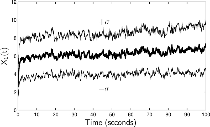
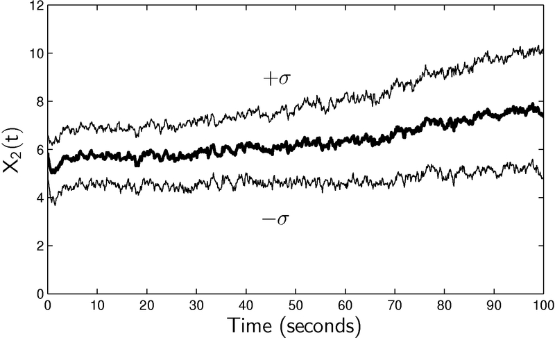
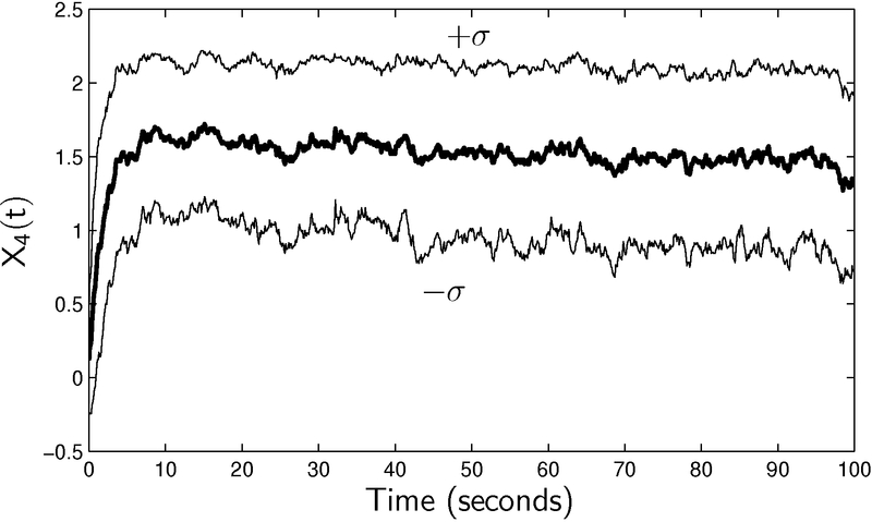
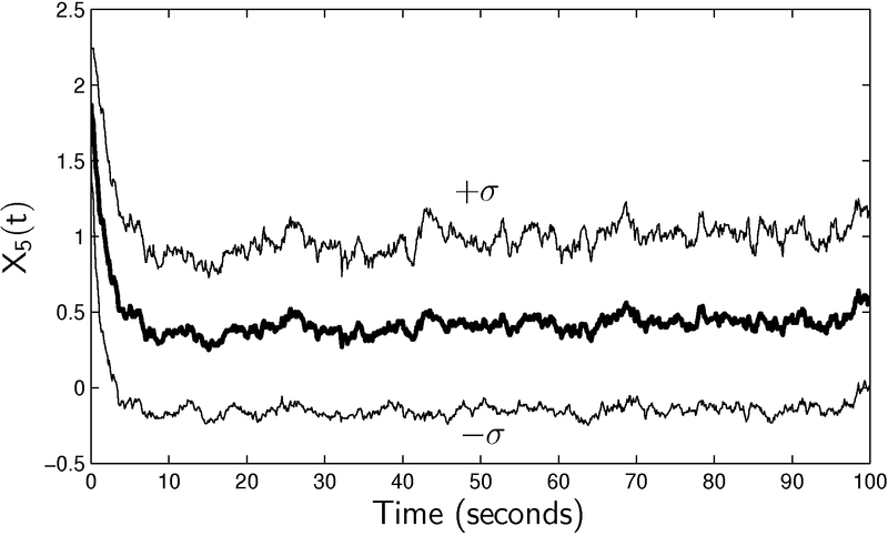
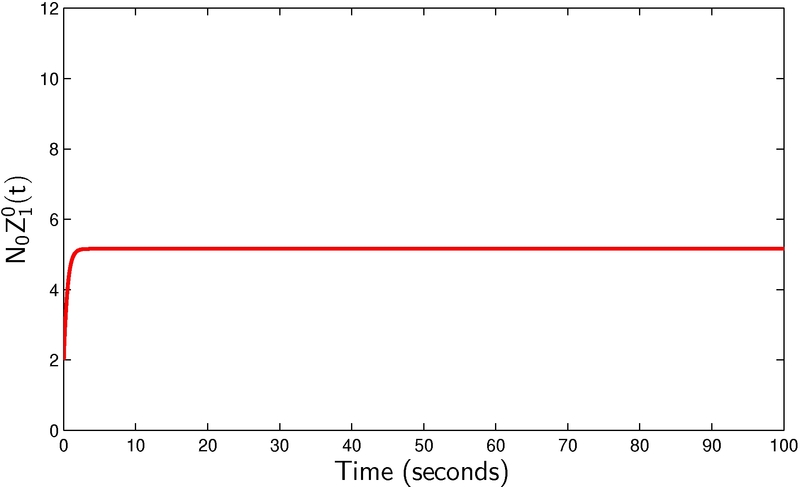
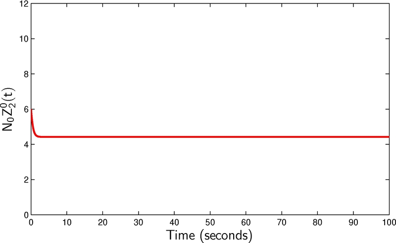
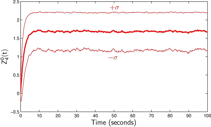
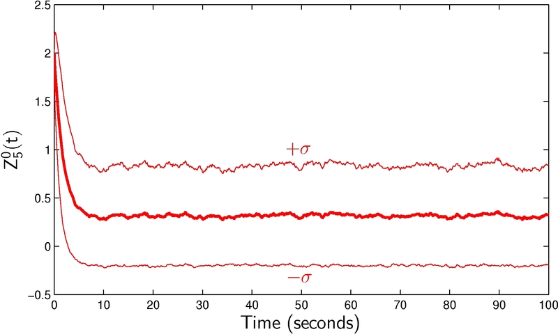
Figure 1: Simulation of the full model during $t=0$ to $t=100$

Figure 2: Approximation using the limiting model for $\gamma=0$ in the alternative scaling

For $\gamma=0$, we observe the evolution of the processes during the time interval $[0,100]$. The full model is reduced to the $4$-dimensional hybrid model (6.5) in which $Z_{1}^{0}$ and $Z_{2}^{0}$ are the solution of a pair of ordinary differential equations and $Z_{4}^{0}$ and $Z_{5}^{0}$ are discrete with transition intensities depending on $Z_{2}^{0}$. The evolution of $X_{1}$, $X_{2}$, $X_{4}$, and $X_{5}$ in the full model is given in Figure 2 and the evolution of the approximation is given in Figure 2. The exact simulations of the full model are done using Gillespie’s stochastic simulation algorithm (SSA) from Gillespie (1977). For the approximation, $Z_{1}^{0}$ and $Z_{2}^{0}$ are solved by the Matlab ODE solver, and $Z_{4}^{0}$ and $Z_{5}^{0}$ are computed by Gillespie’s SSA taking $Z_{2}^{0}$ from the solution of ODE. The evolution of $X_{1}$ and $X_{2}$ are well captured by $Z_{1}^{0}$ and $Z_{2}^{0}$ in Figure 2. These deterministic values approximate the evolution of the mean of $X_{1}$ and $X_{2}$ given in Figure 2 except for a slight increase over time in the simulation of the full model. Note that in the approximate model $Z_{1}^{0}(t)+2Z_{2}^{0}(t)$ is constant, but that is not the case in the full model.

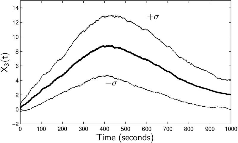
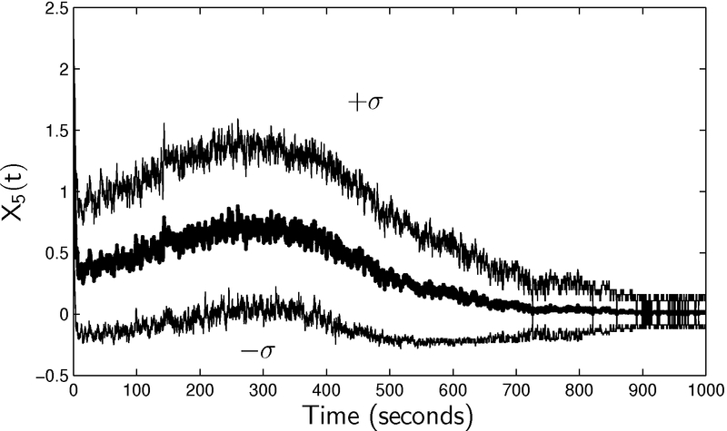
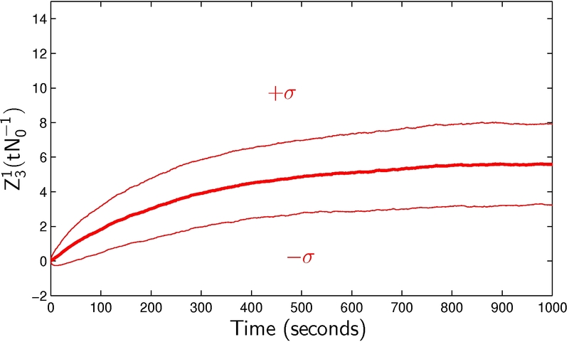
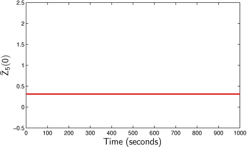
Figure 3: Simulation of the full model during $t=0$ to $t=1000$

Figure 4: Approximation using the limiting model for $\gamma=1$ in the alternative scaling

For $\gamma=1$, we consider the evolution of the processes on the time interval $[0,1000]$. The full model is reduced to the $1$-dimensional limiting system (6.6) with a single jump process $Z_{3}^{1}$. Comparing the governing equations for $Z_{3}^{N,1}$ and $Z_{3}^{1}$, the different behavior of the evolution of the two processes comes from the difference between $Z_{5}^{N,1}$ and $\overline{Z}_{5}^{1}(t)=\frac{\kappa_{5}\varphi_{2}(Z_{12}(0))}{\kappa_{6}+\kappa_{5}\varphi_{2}(Z_{12}(0))}Z_{45}(0)$. Therefore, plots of the evolution of both $X_{3}$ and $X_{5}$ in the exact simulation are given in Figure 4. In Figure 4, the evolution of $Z_{3}^{1}$ and of $\overline{Z}_{5}^{1}$ is given. For both exact and approximate simulations, we use Gillespie’s SSA. In Figure 4, $Z_{5}^{N,1}$ increases slightly and then decreases to zero. Since $\overline{Z}_{5}^{1}$ is approximated as constant in Figure 4, the increase during the early time and the decrease to zero of $X_{3}$ is not captured by the approximation.

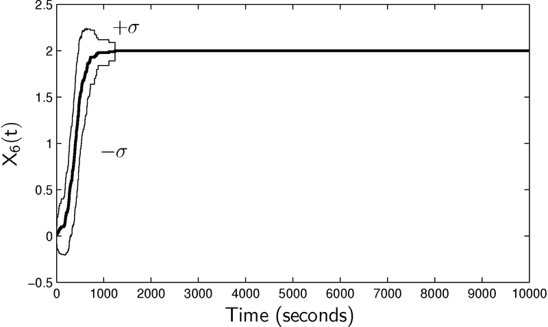
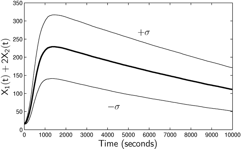
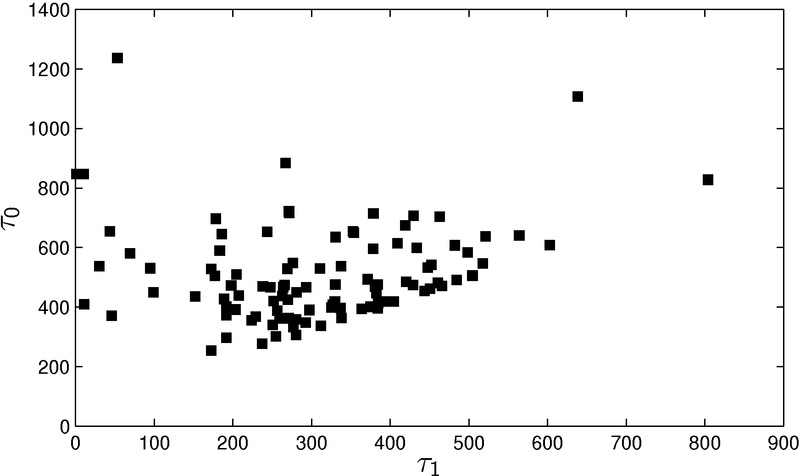
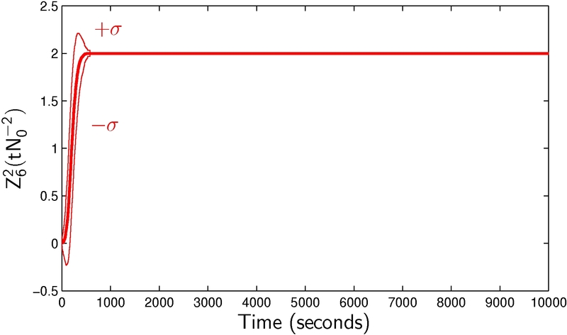
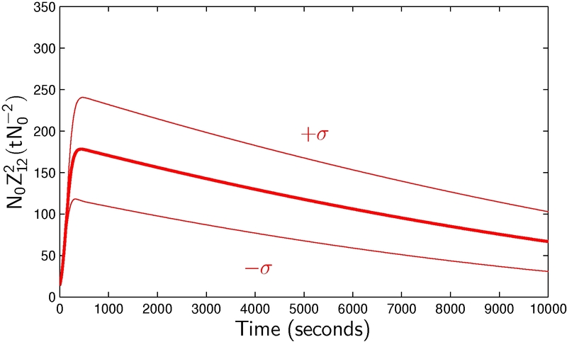
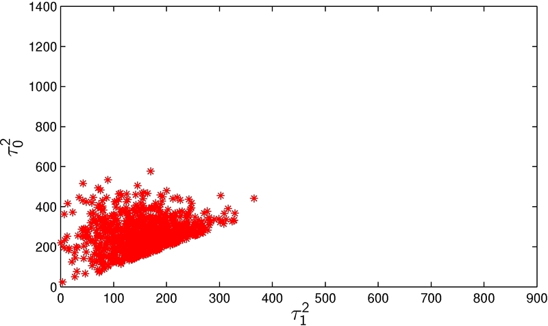
Figure 5: Simulation of the full model during $t=0$ to $t=10000$

Figure 6: Approximation using the limiting model for $\gamma=2$ in the alternative scaling

For $\gamma=2$, the simulation is carried out on the time interval $[0,10000]$. The $3$-dimensional limiting model (6.3) is piecewise deterministic and includes the auxiliary variables $Z_{12}^{2}$, $Z_{45}^{2}$, and the species abundance $Z_{6}^{2}$. $Z_{12}^{2}$ is governed by a random differential equation driven by a component of the jump process, $Z_{45}^{2}$. $Z_{45}^{2}$ and $Z_{6}^{2}$ are discrete with transition intensities that depend on $Z_{12}^{2}$. Since there is mutual dependence between the continuous and discrete components, we modify Gillespie’s SSA to simulate the limiting system. Here is a brief description of the simulation method for the limiting system.

1. Assume that the process has been simulated up to $t_{i}$, the $i$th jump time of the jump process. Simulate a unit exponential random variable $\Delta$ by simulating a uniform $[0,1]$ random number $r_{1}$ and setting $\Delta=\log\frac{1}{r_{1}}$.

2. Solve the differential equation for $Z_{12}^{2}$ starting at $Z_{12}^{2}(t_{i})$ holding $Z_{45}^{2}(t)=Z_{45}^{2}(t_{i})$ and $Z_{6}^{2}(t)=Z_{6}^{2}(t_{i})$ until time $t_{i+1}$ satisfying

   $$\int_{t_{i}}^{t_{i+1}}\big{(}\kappa_{7}\varphi_{2}(Z_{12}^{2}(s))\overline{Z}_{5}^{2}(s)+\kappa_{8}Z_{6}^{2}(s)\big{)}\,ds$$

   $$\qquad\qquad=Z_{45}^{2}(t_{i})\int_{t_{i}}^{t_{i+1}}\frac{\kappa_{5}\kappa_{7}\varphi_{2}(Z_{12}^{2}(s))^{2}}{\kappa_{6}+\kappa_{5}\varphi_{2}(Z_{12}^{2}(s))}ds+\kappa_{8}Z_{6}^{2}(t_{i})(t_{i+1}-t_{i})$$

   $$\qquad\qquad=\Delta.$$

   (We compute the integral by the trapezoid rule using the grid points from the ODE solver.)

3. Simulate a uniform $[0,1]$ random number $r_{2}$. If

   $$r_{2} \leq \frac{\kappa_{7}\varphi_{2}(Z_{12}^{2}(t_{i+1}))\overline{Z}_{5}^{2}(t_{i+1}-)}{\kappa_{7}\varphi_{2}(Z_{12}^{2}(t_{i+1}))\overline{Z}_{5}^{2}(t_{i+1}-)+\kappa_{8}Z_{6}^{2}(t_{i+1}-))}$$

   $$= \frac{\kappa_{5}\kappa_{7}\varphi_{2}(Z_{12}^{2}(t_{i+1}))^{2}Z_{45}^{2}(t_{i})}{\kappa_{5}\kappa_{7}\varphi_{2}(Z_{12}^{2}(t_{i+1}))^{2}Z^{2}_{45}(t_{i})+\kappa_{8}Z_{6}^{2}(t_{i})(\kappa_{6}+\kappa_{5}\varphi_{2}(Z_{12}^{2}(t_{i+1})))},$$

   set

   $$\left(\begin{array}[]{c}Z_{45}^{2}(t_{i+1})\\ Z^{2}_{6}(t_{i+1})\end{array}\right)=\left(\begin{array}[]{c}Z_{45}^{2}(t_{i})\\ Z^{2}_{6}(t_{i})\end{array}\right)+\left(\begin{array}[]{c}-1\\ 1\end{array}\right),$$

   and if the reverse inequality holds in (3), set

   $$\left(\begin{array}[]{c}Z_{45}^{2}(t_{i+1})\\ Z^{2}_{6}(t_{i+1})\end{array}\right)=\left(\begin{array}[]{c}Z_{45}^{2}(t_{i})\\ Z^{2}_{6}(t_{i})\end{array}\right)+\left(\begin{array}[]{c}1\\ -1\end{array}\right).$$

4. Go back to step $1$.

Comparing plots for $X_{1}(t)+2X_{2}(t)$ in Figure 6 and for $N_{0}Z_{12}^{2}(tN_{0}^{-2})$ in Figure 6, the plot in the approximation increases more rapidly at early times and starts to drop earlier than the plot in the exact simulation. Also, the peak level in the approximation is much lower than the peak level in the exact simulation.

Since $\kappa_{8}=8.77\times 10^{-8}$ is small compared to the time interval, Reaction 8 will rarely occur on the time scales we are considering. We retained this reaction in the limiting model only to emphasize that a long time after the model appears to equilibrate, action may restart after the dissociation

$$DNA\cdot 2D\rightharpoonup DNA\cdot D+D.$$

If Reaction 8 does not occur, the stochastic behavior of the limiting model just depends on the two jump times

$$\tau_{1}^{2}=\inf\{t:Z_{45}^{2}(t)=1\},\quad\tau_{0}^{2}=\inf\{t:Z_{45}^{2}(t)=0\},$$

so we compare these random variable to the corresponding variables

$$\tau_{1}=\inf\{t:X_{4}(t)+X_{5}(t)=1\},\quad\tau_{0}=\inf\{t:X_{4}(t)+X_{5}(t)=0\},$$

from the original model or more precisely, because of the change of time scale, we compare $(N_{0}^{2}\tau_{1}^{2},N_{0}^{2}\tau_{2}^{2})$ to $(\tau_{1},\tau_{2})$.

In Figure 6, plots for $\tau_{1}$ and $\tau_{0}$ for $100$ exact simulations are given. Taking the average, the mean of first hitting time of $X_{4}(t)+X_{5}(t)$ to $1$ is $305.44$ and the mean of the first hitting time of $X_{4}(t)+X_{5}(t)$ to $0$ is $512.45$. In Figure 6, plots for 1000 simulations of $\tau_{1}^{2}$ and $\tau_{0}^{2}$ are given. The mean of the first hitting time of $Z_{45}^{2}(tN_{0}^{-2})$ to $1$ is $155.95$ and the mean of the first hitting time of $Z_{45}^{2}(tN_{0}^{-2})$ to $0$ is $261.01$. Comparing the two stopping times in the simulations of the full model and of the approximation, the mean hitting time to $1$ and $0$ in the approximation is much faster than in the full model. Consequently, the quicker decrease of $Z_{45}^{2}$ to $0$ gives a discrepancy in the peak levels and the peak times in the full model and in the approximation.

6.4 Derivation of Michaelis-Menten equation

Darden (1979, 1982) derives the Michaelis-Menten equation from a stochastic reaction network model. His result can be obtained as a special case of the methods developed here.

Consider the reaction system

$$S_{1}+S_{2}\mathop{\rightleftharpoons}^{\kappa_{1}^{\prime}}_{\kappa_{2}^{\prime}}S_{3}\mathop{\rightharpoonup}^{\kappa_{3}^{\prime}}S_{4}+S_{2},$$

where $S_{1}$ is the substrate, $S_{2}$ the enzyme, $S_{3}$ the enzyme-substrate complex, and $S_{4}$ the product. Assume that the parameters scale so that

$$Z^{N}_{1}(t) = Z^{N}_{1}(0)-N^{-1}Y_{1}(N\int_{0}^{t}\kappa_{1}Z^{N}_{1}(s)Z^{N}_{2}(s)ds)+N^{-1}Y_{2}(N\int_{0}^{t}\kappa_{2}Z^{N}_{3}(s)ds)$$

$$Z^{N}_{2}(t) = Z^{N}_{2}(0)-Y_{1}(N\int_{0}^{t}\kappa_{1}Z^{N}_{1}(s)Z^{N}_{2}(s)ds)+Y_{2}(N\int_{0}^{t}\kappa_{2}Z^{N}_{3}(s)ds)$$

$$\qquad+Y_{3}(N\int_{0}^{t}\kappa_{3}Z^{N}_{3}(s)ds)$$

$$Z_{3}^{N}(t) = Z^{N}_{2}(0)+Y_{1}(N\int_{0}^{t}\kappa_{1}Z^{N}_{1}(s)Z^{N}_{2}(s)ds)-Y_{2}(N\int_{0}^{t}\kappa_{2}Z^{N}_{3}(s)ds)$$

$$\qquad-Y_{3}(N\int_{0}^{t}\kappa_{3}Z^{N}_{3}(s)ds)$$

$$Z^{N}_{4}(t) = N^{-1}Y_{3}(N\int_{0}^{t}\kappa_{3}Z^{N}_{3}(s)ds),$$

that is, $\alpha_{1}=\alpha_{4}=1$, $\alpha_{2}=\alpha_{3}=0$, $\beta_{1}=0$, and $\beta_{2}=\beta_{3}=1$.

Note that $M=Z^{N}_{3}(t)+Z^{N}_{2}(t)$ is constant, and define

$$V_{2}^{N}(t)=\int_{0}^{t}Z_{2}^{N}(s)ds.$$

Theorem 6.1

Assume that $Z^{N}_{1}(0)\rightarrow x_{A}(0)$. Then $(Z^{N}_{1},V^{N}_{2})$ converges to $(x_{1}(t),v_{2}(t))$ satisfying

$$x_{1}(t) = x_{1}(0)-\int_{0}^{t}\kappa_{1}x_{1}(s)\dot{v}_{2}(s)ds+\int_{0}^{t}\kappa_{2}(M-\dot{v}_{2}(s))ds$$ (6.8)

$$0 = -\int_{0}^{t}\kappa{}_{1}x_{1}(s)\dot{v}_{2}(s)ds+\int_{0}^{t}(\kappa_{2}+\kappa_{3})(M-\dot{v}_{2}(s))ds,$$

and hence $\dot{v}_{2}(s)=\frac{(\kappa_{2}+\kappa_{3})M}{\kappa_{2}+\kappa_{3}+\kappa_{1}x_{1}(s)}$ and

$$\dot{x}_{1}(t)=-\frac{M\kappa_{1}\kappa_{3}x_{1}(t)}{\kappa_{2}+\kappa_{3}+\kappa_{1}x_{1}(s)}.$$

Proof. Relative compactness of the sequence $(Z_{1}^{N},V_{2}^{N})$ is straightforward. Dividing the second equation by $N$ and passing to the limit, we see that any limit point $(x_{1},v_{2})$ of $(Z_{1}^{N},V_{2}^{N})$ must satisfy

$$0=-\int_{0}^{t}\kappa{}_{1}x_{1}(s)dv_{2}(s)+(\kappa_{2}+\kappa_{3})Mt-\int_{0}^{t}(\kappa_{2}+\kappa_{3})dv_{2}(s).$$ (6.9)

Since $v_{2}$ is Lipschitz, it is absolutely continuous, and rewriting (6.9) in terms of the derivative gives the second equation in (6.8). The first equation follows by a similar argument. $\Box$

6.5 Limiting models when the balance conditions fail

The balance condition, Condition 3.2, has as its goal ensuring that the normalized species numbers remain positive, at least on average, and bounded. Mastny, Haseltine, and Rawlings (2007) consider examples in which model reduction is achieved by eliminating species whose numbers are zero most of the time. We translate some of their examples into our notation and see how one can obtain reduced models even though the balance conditions fail.

Consider

$$S_{1}\mathop{\rightleftharpoons}^{\kappa^{\prime}_{1}}_{\kappa^{\prime}_{2}}2S_{2},\quad S_{2}\mathop{\rightharpoonup}^{\kappa^{\prime}_{3}}S_{3},$$

where we assume $\kappa_{2}^{\prime},\kappa_{3}^{\prime}>>\kappa_{1}^{\prime}$. We take the scaled system to be

$$Z_{1}^{N}(t) = Z_{1}(0)-Y_{1}(\int_{0}^{t}\kappa_{1}Z_{1}^{N}(s)ds)+Y_{2}(N\int_{0}^{t}\kappa_{2}Z_{2}^{N}(s)(Z_{2}^{N}(s)-1)ds)$$

$$Z_{2}^{N}(t) = Z_{2}(0)+2Y_{1}(\int_{0}^{t}\kappa_{1}Z_{1}^{N}(s)ds)-2Y_{2}(N\int_{0}^{t}\kappa_{2}Z_{2}^{N}(s)(Z_{2}^{N}(s)-1)ds)-Y_{3}(N\int_{0}^{t}\kappa_{3}Z_{2}^{N}(s)ds)$$

$$Z_{3}^{N}(t) = Z_{3}(0)+Y_{3}(N\int_{0}^{t}\kappa_{3}Z_{2}^{N}(s)ds).$$

Consequently, assuming $Z_{2}^{N}(0)=0$, for most $t>0$, $Z^{N}_{2}(t)=0$ and

$$2Y_{1}(\int_{0}^{t}\kappa_{1}Z_{1}^{N}(s)ds)=Y_{3}(N\int_{0}^{t}\kappa_{3}Z_{2}^{N}(s)ds)+2Y_{2}(N\int_{0}^{t}\kappa_{2}Z_{2}^{N}(s)(Z_{2}^{N}(s)-1)ds).$$

To be precise, letting $\varLambda$ denote Lebesgue measure and defining

$$\widehat{R}^{N}_{2}(t)=\int_{0}^{t}{\bf 1}_{\{Z_{2}^{N}(r-)=2\}}dR_{2}^{N}(r),\quad\widehat{R}_{3}^{N}(t)=\int_{0}^{t}{\bf 1}_{\{Z_{2}^{N}(r-)=2\}}dR_{3}^{N}(r),$$

for each $t>0$,

$$\lim_{N\rightarrow\infty}\varLambda\{0\leq s\leq t:Z^{N}_{2}(s)\neq 0\}\leq\lim_{N\rightarrow\infty}\int_{0}^{t}Z^{N}_{2}(s)ds = 0$$

$$\limsup_{N\rightarrow\infty}\sup_{s\leq t}Z_{2}^{N}(s) \leq 2$$

$$\lim_{N\rightarrow\infty}\int_{0}^{t}|R_{2}^{N}(s)-\widehat{R}_{2}^{N}(s)|ds = 0$$

$$\lim_{N\rightarrow\infty}\int_{0}^{t}|R_{3}^{N}(s)-2\widehat{R}_{3}^{N}(s)|ds = 0$$

so

$$\lim_{N\rightarrow\infty}\int_{0}^{t}|R_{1}^{N}(s)-\widehat{R}_{2}^{N}(s)-\widehat{R}_{3}^{N}(s)|ds=0.$$

Setting $Q^{N}(t)={\bf 1}_{\{Z_{2}^{N}(t)=2\}}$,

$$\widehat{R}_{2}^{N}(t)-\int_{0}^{t}NQ^{N}(s)\kappa_{2}2ds\mbox{\rm\ and }\widehat{R}_{3}^{N}(t)-\int_{0}^{t}NQ^{N}(s)\kappa_{3}2ds$$

are martingales. Working first with a subsequence satisfying (A.7), by Lemma A.13, $(\widehat{R}_{2}^{N},\widehat{R}_{3}^{N})$ converges to counting processes $(\widehat{R}_{2},\widehat{R}_{3})$ with intensities

$$\widehat{\lambda}_{2}(t)=\frac{\kappa_{1}\kappa_{2}}{\kappa_{2}+\kappa_{3}}Z_{1}(t),\quad\widehat{\lambda}_{3}(t)=\frac{\kappa_{1}\kappa_{3}}{\kappa_{2}+\kappa_{3}}Z_{1}(t),$$

where $Z_{1}(t)=Z_{1}(0)-\widehat{R}_{3}(t)$. It follows that the finite dimensional distributions of $(Z_{1}^{N},Z_{3}^{N})$ converge to those of a solution to

$$Z_{1}(t) = Z_{1}(0)-Y(\int_{0}^{t}\frac{\kappa_{1}\kappa_{3}}{\kappa_{2}+\kappa_{3}}Z_{1}(s)ds)$$

$$Z_{3}(t) = Z_{3}(0)+2Y(\int_{0}^{t}\frac{\kappa_{1}\kappa_{3}}{\kappa_{2}+\kappa_{3}}Z_{1}(s)ds),$$

which is the reduced model obtained in Mastny et al. (2007). More precisely, $(Z_{1}^{N},Z_{3}^{N})$ converges in the Jakubowski topology as described in Remark A.14

(Note the relationship between our rate constants and those of Mastny et al. (2007): $\kappa_{1}=k_{1}$, $\kappa_{2}=\frac{1}{2}k_{-1}$, and $\kappa_{3}=k_{2}$.)

Appendix A Appendix

A.1 Convergence of random measures

The material in this section is taken from Kurtz (1992). Proofs of the results can be found there.

Let $({\mathbb{L}},d)$ be a complete, separable metric space, and let ${\cal M}({\mathbb{L}})$ be the space of finite measures on ${\mathbb{L}}$ with the weak topology. The Prohorov metric on ${\cal M}({\mathbb{L}})$ is defined by

$$\rho(\mu,\nu)=\inf\{\epsilon>0:\mu(B)\leq\nu(B^{\epsilon})+\epsilon,\nu(B)\leq\mu(B^{\epsilon})+\epsilon,B\in{\cal B}({\mathbb{L}})\},$$ (A.1)

where $B^{\epsilon}=\{x\in{\mathbb{L}}:\inf_{y\in B}d(x,y)<\epsilon\}$. The following lemma is a simple consequence of Prohorov’s theorem.

Lemma A.1

Let $\{\Gamma_{n}\}$ be a sequence of ${\cal M}({\mathbb{L}})$-valued random variables. Then $\Gamma_{n}$ is relatively compact if and only if $\{\Gamma_{n}({\mathbb{L}})\}$ is relatively compact as a family of ${\mathbb{R}}$-valued random variables and for each $\epsilon>0$, there exists a compact $K\subset{\mathbb{L}}$ such that $\sup_{n}P\{\Gamma_{n}(K^{c})>\epsilon\}<\epsilon$.

Corollary A.2

Let $\{\Gamma_{n}\}$ be a sequence of ${\cal M}({\mathbb{L}})$-valued random variables. Suppose that $\sup_{n}E[\Gamma_{n}({\mathbb{L}})]<\infty$ and that for each $\epsilon>0$, there exists a compact $K\subset{\mathbb{L}}$ such that

$$\limsup_{n\rightarrow\infty}E[\Gamma_{n}(K^{c})]\leq\epsilon.$$

Then $\{\Gamma_{n}\}$ is relatively compact.

Let ${\cal L}({\mathbb{L}})$ be the space of measures on ${\mathbb{L}}\times[0,\infty)$ such that $\mu$$({\mathbb{L}}\times[0,t])<\infty$ for each $t>0$, and let ${\cal L}_{m}({\mathbb{L}})\subset{\cal L}({\mathbb{L}})$ be the subspace on which $\mu({\mathbb{L}}\times[0,t])=t$. For $\mu\in{\cal L}({\mathbb{L}})$, let $\mu^{t}$ denote the restriction of $\mu$ to ${\mathbb{L}}\times[0,t]$. Let $\rho_{t}$ denote the Prohorov metric on ${\cal M}({\mathbb{L}}\times[0,t])$, and define $\widehat{\rho}$ on ${\cal L}({\mathbb{L}})$ by

$$\widehat{\rho}(\mu,\nu)=\int_{0}^{\infty}e^{-t}1\wedge\rho_{t}(\mu^{t},\nu^{t})dt,$$

that is, $\{\mu_{n}\}$ converges in $\widehat{\rho}$ if and only if $\{\mu_{n}^{t}\}$ converges weakly for almost every $t$. In particular, if $\widehat{\rho}(\mu_{n},\mu)\rightarrow 0$, then $\rho_{t}(\mu_{n}^{t},\mu^{t})\rightarrow 0$ if and only if $\mu_{n}({\mathbb{L}}\times[0,t])\rightarrow\mu({\mathbb{L}}\times[0,t])$. The following lemma is an immediate consequence of Lemma A.1.

Lemma A.3

A sequence of $({\cal L}_{m}({\mathbb{L}}),\widehat{\rho})$-valued random variables $\{\Gamma_{n}\}$ is relatively compact if and only if for each $\epsilon>0$ and each $t>0$, there exists a compact $K\subset{\mathbb{L}}$ such that $\inf_{n}E[\Gamma_{n}(K\times[0,t])]\geq(1-\epsilon)t$.

Lemma A.4

Let $\Gamma$ be an $({\cal L}({\mathbb{L}}),\widehat{\rho})$-valued random variable adapted to a complete filtration $\{{\cal F}_{t}\}$ in the sense that for each $t\geq 0$ and $H\in{\cal B}({\mathbb{L}})$, $\Gamma(H\times[0,t])$ is ${\cal F}_{t}$-measurable. Let $\lambda(G)=\Gamma({\mathbb{L}}\times G)$. Then there exists an $\{{\cal F}_{t}\}$-optional, ${\cal P}({\mathbb{L}})$-valued process $\gamma$ such that

$$\int_{{\mathbb{L}}\times[0,t]}h(y,s)\Gamma(dy\times ds)=\int_{0}^{t}\int_{{\mathbb{L}}}h(y,s)\gamma_{s}(dy)\lambda(ds)$$ (A.2)

for all $h\in B({\mathbb{L}}\times[0,\infty))$ with probability one. If $\lambda([0,t])$ is continuous, then $\gamma$ can be taken to be $\{{\cal F}_{t}\}$-predictable.

Lemma A.5

Let $\{(x_{n},\mu_{n})\}\subset D_{{\mathbb{E}}}[0,\infty)\times{\cal L}({\mathbb{L}})$, and $(x_{n},\mu_{n})\rightarrow(x,\mu)$. Let $h\in C({\mathbb{E}}\times{\mathbb{L}})$ and $\psi$ be a nonnegative function on $[0,\infty)$ satisfying $\lim_{r\rightarrow\infty}\psi(r)/r=\infty$ such that

$$\sup_{n}\int_{{\mathbb{L}}\times[0,t]}\psi(|h(x_{n}(s),y)|)\mu_{n}(dy\times ds)<\infty$$ (A.3)

for each $t>0$.

Define

$$u_{n}(t)=\int_{{\mathbb{L}}\times[0,t]}h(x_{n}(s),y)\mu_{n}(dy\times ds),\quad u(t)=\int_{{\mathbb{L}}\times[0,t]}h(x(s),y)\mu(dy\times ds)$$

$z_{n}(t)=\mu_{n}({\mathbb{L}}\times[0,t])$, and $z(t)=\mu({\mathbb{L}}\times[0,t])$.

• If $x$ is continuous on $[0,t]$ and $\lim_{n\rightarrow\infty}z_{n}(t)=z(t)$, then $\lim_{n\rightarrow\infty}u_{n}(t)=u(t)$.

• If $(x_{n},z_{n},\mu_{n})\rightarrow(x,z,\mu)$ in $D_{{\mathbb{E}}\times{\mathbb{R}}}[0,\infty)\times{\cal L}({\mathbb{L}})$, then $(x_{n},z_{n},u_{n},\mu_{n})\rightarrow(x,z,u,\mu)$ in $D_{{\mathbb{E}}\times{\mathbb{R}}\times{\mathbb{R}}}[0,\infty)\times{\cal L}({\mathbb{L}})$. In particular, $\lim_{n\rightarrow\infty}u_{n}(t)=u(t)$ at all points of continuity of $z$.

• The continuity assumption on $h$ can be replaced by the assumption that $h$ is continuous a.e. $\nu_{t}$ for each $t$, where $\nu_{t}\in{\cal M}({\mathbb{E}}\times{\mathbb{L}})$ is the measure determined by $\nu_{t}(A\times B)=\mu\{(y,s):x(s)\in A,s\leq t,y\in B\}$.

The Lemma A.5 and the continuous mapping theorem give the following.

Lemma A.6

Suppose $(Z^{N},V^{N})\Rightarrow(Z,V)$ in $D_{{\mathbb{E}}}[0,\infty)\times{\cal L}_{m}({\mathbb{L}})$. Let $h\in C({\mathbb{E}}\times{\mathbb{L}})$ and $\psi$ be as in Lemma A.5. If $\{\int_{0}^{t}\psi(|h(Z^{N}(s),y)|)V^{N}(dy\times ds)\}$is stochastically bounded for all $t>0$, then

$$\int_{{\mathbb{L}}\times[0,\cdot]}h(Z^{N}(s),y)V^{N}(dy\times ds)\Rightarrow\int_{{\mathbb{L}}\times[0,\cdot]}h(Z(s),y))V(dy\times ds).$$

A.2 Martingale properties of counting processes

A cadlag stochastic process $R$ is a counting process if $R(0)=0$ and $R$ is constant except for jumps of plus one. If $R$ is adapted to a filtration $\{{\cal F}_{t}\}$, then a nonnegative $\{{\cal F}_{t}\}$-adapted process $\lambda$ is an $\{{\cal F}_{t}\}$-intensity for $R$ if

$$M(t)=R(t)-\int_{0}^{t}\lambda(s)ds$$

is an $\{{\cal F}_{t}\}$-local martingale. Specifically, letting $\tau_{l}$ denote the $l$th jump time of $R$,

$$M^{\tau_{l}}(t)\equiv M(t\wedge\tau_{l})=R(t\wedge\tau_{l})-\int_{0}^{t\wedge\tau_{l}}\lambda(s)ds$$

is an $\{{\cal F}_{t}\}$-martingale for each $l$.

For simplicity, we assume that $\lambda$ is cadlag.

Remark A.7

For $R_{k}$ defined in (2.1) and $\{{\cal F}_{t}\}=\sigma(R_{l}(s):s\leq t,l=1,\ldots,r_{0})$, the intensity for $R_{k}$ is $t\rightarrow\lambda_{k}(X(t))$.

Lemma A.8

For each $t\geq 0$ and each $l$,

$$l\geq E[R(t\wedge\tau_{l})]=E[\int_{0}^{t\wedge\tau_{l}}\lambda(s)ds]$$ (A.4)

and

$$E[R(t)]=E[\int_{0}^{t}\lambda(s)ds],$$

where we allow $\infty=\infty$. If $E[R(t)]<\infty$ for all $t>0$, then

$$R(t)-\int_{0}^{t}\lambda(s)ds$$

is an $\{{\cal F}_{t}\}$-martingale.

Two counting processes, $R_{1}$, $R_{2}$, are orthogonal if they have no simultaneous jumps.

Lemma A.9

Let $R_{1},\ldots,R_{m}$ be pairwise orthogonal $\{{\cal F}_{t}\}$-adapted counting processes with $\{{\cal F}_{t}\}$-intensities $\lambda_{k}$. Then, perhaps on a larger probability space, there exist independent unit Poisson processes $Y_{1},\ldots,Y_{m}$ such that

$$R_{k}(t)=Y_{k}(\int_{0}^{t}\lambda_{k}(s)ds),$$

and $R=\sum_{k=1}^{m}R_{k}$ is a counting process with intensity $\lambda=\sum_{k=1}^{m}\lambda_{k}$.

If $\tau_{l}$ is the $l$th jump time of $R$, then

$$P\{R_{k}(\tau_{l})-R_{k}(\tau_{l}-)=1|{\cal F}_{\tau_{l}}\}=\frac{\lambda_{k}(\tau_{l}-)}{\lambda(\tau_{l}-)}.$$ (A.5)

Remark A.10

Note that the right side of (A.5) involves the left limits of the intensities. If the intensities are not cadlag, then $\lambda_{k}(\tau_{l}-)$ should be replaced by

$$\limsup_{h\rightarrow 0+}h^{-1}\int_{\tau_{l}-h}^{\tau_{l}}\lambda_{k}(s)ds.$$

The intensity of a counting process does not necessarily uniquely determined its distribution. For example, consider the system

$$R_{1}(t) = Y_{1}(\int_{0}^{t}\lambda(R_{1}(s))ds)$$

$$R_{2}(t) = Y_{2}(\int_{0}^{t}\lambda(R_{1}(s))ds).$$

The intensity for each component is $\lambda(R_{1}(t))$, but the two components will not have the same distribution.

Proof. See Meyer (1971) and Kurtz (1980). $\Box$

Lemma A.11

Suppose that $R_{1}^{N},\ldots,R_{m}^{N}$ are pairwise orthogonal counting processes adapted to a filtration $\{{\cal F}_{t}^{N}\}$ with $\{{\cal F}_{t}^{N}\}$-intensities $\lambda_{1}^{N},\ldots,\lambda_{m}^{N}$. Let $\Lambda_{k}^{N}(t)=\int_{0}^{t}\lambda_{k}^{N}(s)ds$, and suppose that $(\Lambda_{1}^{N},\ldots,\Lambda_{m}^{N})\Rightarrow(\Lambda_{1},\ldots,\Lambda_{m})$ in the Skorohod topology on $D_{{\mathbb{R}}^{m}}[0,\infty)$. Then $\{(R_{1}^{N},\ldots,R_{m}^{N})\}$ is relatively compact in the Skorohod topology and any limit point $(R_{1},\ldots,R_{m})$ consists of pairwise orthogonal counting processes.

At least along a further subsequence,

$$(\Lambda_{1}^{N},\ldots,\Lambda_{m}^{N},R_{1}^{N},\ldots,R_{m}^{N})\Rightarrow(\Lambda_{1},\ldots,\Lambda_{m},R_{1},\ldots,R_{m}),$$

and letting $\{{\cal F}_{t}^{\Lambda,R}\}$ be the filtration generated by $(\Lambda_{1},\ldots,\Lambda_{m},R_{1},\ldots,R_{m})$, $R_{k}-\Lambda_{k}$ are $\{{\cal F}_{t}^{\Lambda,R}\}$-local martingales and there exist independent unit Poisson processes $(Y_{1},\ldots,Y_{m})$ such that

$$R_{k}(t)=Y_{k}(\Lambda_{k}(t)),\quad k=1,\ldots,m.$$ (A.6)

Remark A.12

If the $\Lambda_{k}$ are adapted to $\{{\cal F}_{t}^{R}\}$, then $R$ will be the unique solution of (A.6) and $R^{N}\Rightarrow R$ in the Skorohod topology.

Proof. See Kabanov, Liptser, and Shiryaev (1984). $\Box$

In Section 6.5, we consider an example for which the integrated intensities did not have a continuous limit. The next lemma covers that situation.

Lemma A.13

Suppose that $R_{0}^{N},R_{1}^{N},\ldots,R_{m}^{N}$ are counting processes adapted to a filtration $\{{\cal F}_{t}^{N}\}$, and $R_{1}^{N},\ldots,R_{m}^{N}$ are pairwise orthogonal. Suppose $R_{0}^{N}$ has $\{{\cal F}_{t}^{N}\}$-intensity $\lambda_{0}^{N}$, and $R_{1}^{N},\ldots,R_{m}^{N}$ have $\{{\cal F}_{t}^{N}\}$-intensities $\lambda_{k}^{N}=NQ^{N}\mu_{k}^{N}$, where $Q^{N}\geq 0$. Suppose

$$(\lambda_{0}^{N},\mu_{1}^{N},\ldots,\mu_{m}^{N})\Rightarrow(\lambda_{0},\mu_{1},\ldots,\mu_{m}),$$ (A.7)

and

$$\int_{0}^{t}|R_{0}^{N}(s)-\sum_{k=1}^{m}R_{k}^{N}(s)|ds\rightarrow 0,$$ (A.8)

for each $t>0$. Then $\{(R_{0}^{N},R_{1}^{N},\ldots,R_{m}^{N})\}$ is relatively compact in the Jakubowski topology and for any limit point $(R_{0},R_{1},\ldots,R_{m})$,

$$R_{0}=\sum_{k=1}^{m}R_{k},$$

and $R_{1},\ldots,R_{m}$ are pairwise orthogonal counting processes with intensities

$$\lambda_{k}(t)=\frac{\mu_{k}(t)}{\sum_{l=1}^{m}\mu_{l}(t)}\lambda_{0}(t).$$

Remark A.14

The sequence may not be relatively compact in the Skorohod topology since we have not ruled out the possibility that the sequence has discontinuities that coalesce. See the example in Section 6.5.

The Meyer-Zheng conditions (Meyer and Zheng (1984)) imply relative compactness in the Jakubowski topology (Jakubowski (1997)). A sequence of cadlag functions $\{x_{n}\}$ converges to a cadlag function $x$ in the Jakubowski topology if and only if there exists a sequence of time changes $\{\gamma_{n}\}$ such that $(x_{n}\circ\gamma_{n},\gamma_{n})\rightarrow(x\circ\gamma,\gamma)$ in the Skorohod topology. (See Kurtz (1991).) The time-changes are continuous, nondecreasing mappings from $[0,\infty)$ onto $[0,\infty)$ but are not necessarily strictly increasing. Convergence implies $\int_{0}^{t}|x_{n}(s)-x(s)|\wedge 1ds\rightarrow 0$. In contrast to the Skorohod topology, if $x_{n}\rightarrow x$ and $y_{n}\rightarrow y$ in the Jakubowski topology, then $(x_{n},y_{n})\rightarrow(x,y)$ in the Jakubowski topology on cadlag functions in the product space.

Proof. By Lemma A.11, $\{R_{0}^{N}\}$ is relatively compact in the Skorohod topology and hence in the Jakubowski topology. Let

$$\widehat{R}_{0}^{N}=\sum_{k=1}^{m}R_{k}^{N}.$$

The stochastic boundedness of $\{R_{0}^{N}(t)\}$ for each $t>0$ and (A.8) imply the stochastic boundedness of $\{\widehat{R}_{0}^{N}(t)\}$ for each $t>0$ which by (A.4) implies the stochastic boundedness of

$$\{\int_{0}^{t}NQ^{N}(s)\sum_{k=1}^{m}\mu_{k}^{N}(s)ds\}.$$

Let $\gamma_{N}$ be defined by

$$\int_{0}^{\gamma_{N}(t)}(1+NQ^{N}(s)\sum_{k=1}^{m}\mu_{k}^{N}(s))ds=t.$$

Since $|\gamma_{N}(s)-\gamma_{N}(t)|\leq|s-t|$, $\{\gamma_{N}\}$ is relatively compact. Define

$$\Lambda_{k}^{N}(t)=\int_{0}^{t}\lambda_{k}^{N}(s)ds,$$

and observe that

$$\Lambda_{l}^{N}\circ\gamma_{N}(t)=\int_{0}^{t}\frac{NQ^{N}\circ\gamma_{N}(s)\mu_{l}^{N}\circ\gamma_{N}(s)}{1+NQ^{N}\circ\gamma_{N}(s)\sum_{k}\mu_{k}^{N}\circ\gamma_{N}(s)}ds$$

is also Lipschitz with Lipschitz constant $1$. Since $\{\gamma_{N}(t),t\geq 0\}$ are stopping times,

$$R_{l}^{N}-\Lambda_{l}^{N}\circ\gamma_{N}$$

are martingales with respect to the filtration $\{{\cal F}_{\gamma_{N}(t)}^{N}\}$.

The Lipschitz properties imply the relative compactness of $\{(\Lambda_{1}^{N}\circ\gamma_{N},\ldots,\Lambda_{m}^{N}\circ\gamma_{N},\gamma_{N})\}$ in the Skorohod topology which in turn, by Lemma A.11, implies the relative compactness of

$$\{(\Lambda_{1}^{N}\circ\gamma_{N},\ldots,\Lambda_{m}^{N}\circ\gamma_{N},\gamma_{N},R_{1}^{N}\circ\gamma_{N},\ldots,R_{m}^{N}\circ\gamma_{N})\}.$$

Relative compactness of this sequence in the Skorohod topology ensures relative compactness of $\{(R_{1}^{N},\ldots,R_{m}^{N})\}$ in the Jakubowski topology which in turn implies relative compactness of $\{(R_{0}^{N},R_{1}^{N},\ldots,R_{m}^{N})\}$ in the Jakubowski topology.

Along an appropriate subsequence, we have convergence of $\gamma_{N}$ to a limit $\gamma$,

$$\int_{0}^{t}\frac{NQ^{N}\circ\gamma_{N}(s)\sum_{k}\mu_{k}^{N}\circ\gamma_{N}(s)}{1+NQ^{N}\circ\gamma_{N}(s)\sum_{k}\mu_{k}^{N}\circ\gamma_{N}(s)}ds\Rightarrow\widehat{\Lambda},$$

convergence of $\Lambda_{k}^{N}\circ\gamma_{N}$ to

$$\widehat{\Lambda}_{k}(t)=\int_{0}^{t}\frac{\mu_{k}\circ\gamma(s)}{\sum_{l}\mu_{l}\circ\gamma(s)}d\widehat{\Lambda}(ds),$$

and convergence of $(R^{N}_{0},R_{1}^{N},\ldots,R_{m}^{N})$ in the Jakubowski topology to a process satisfying

$$R_{0}=\sum_{k=1}^{m}R_{k}.$$

Since $R_{0}\circ\gamma(t)-\int_{0}^{\gamma(t)}\lambda_{0}(s)ds$ is a martingale, we must have

$$\int_{0}^{\gamma(t)}\lambda_{0}(s)ds=\widehat{\Lambda}(t)$$

and

$$\widehat{\Lambda}_{k}(t)=\int_{0}^{t}\frac{\mu_{k}\circ\gamma(s)}{\sum_{l}\mu_{l}\circ\gamma(s)}\lambda_{0}\circ\gamma(s)\gamma^{\prime}(s)ds.$$

Since $R_{0}$ is a counting process, the $R_{k}$, $k=1,\ldots,m$, must be orthogonal, and $R_{k}$ must have intensity $\frac{\mu_{k}}{\sum_{l}\mu_{l}}\lambda_{0}$. $\Box$

References

- Ball et al. (2006) Karen Ball, Thomas G. Kurtz, Lea Popovic, and Greg Rempala. Asymptotic analysis of multiscale approximations to reaction networks. Ann. Appl. Probab., 16(4):1925–1961, 2006. ISSN 1050-5164.
- Cao et al. (2005) Yang Cao, Daniel T. Gillespie, and Linda R. Petzold. The slow-scale stochastic simulation algorithm. The Journal of Chemical Physics, 122(1):014116, 2005. URL http://link.aip.org/link/?JCP/122/014116/1.
- Crudu et al. (2009) Alina Crudu, Arnaud Debussche, and Ovidiu Radulescu. Hybrid stochastic simplifications for multiscale gene networks. BMC Systems Biology, 3:89, 2009. doi: 10.1186/1752-0509-3-89.
- Darden (1979) Thomas Darden. A pseudo-steady state approximation for stochastic chemical kinetics. Rocky Mountain J. Math., 9(1):51–71, 1979. ISSN 0035-7596. Conference on Deterministic Differential Equations and Stochastic Processes Models for Biological Systems (San Cristobal, N.M., 1977).
- Darden (1982) Thomas A. Darden. Enzyme kinetics: stochastic vs. deterministic models. In Instabilities, bifurcations, and fluctuations in chemical systems (Austin, Tex., 1980), pages 248–272. Univ. Texas Press, Austin, TX, 1982.
- Davis (1993) M. H. A. Davis. Markov models and optimization, volume 49 of Monographs on Statistics and Applied Probability. Chapman & Hall, London, 1993. ISBN 0-412-31410-X.
- E et al. (2005) Weinan E, Di Liu, and Eric Vanden-Eijnden. Nested stochastic simulation algorithm for chemical kinetic systems with disparate rates. The Journal of Chemical Physics, 123(19):194107, 2005. URL http://link.aip.org/link/?JCP/123/194107/1.
- E et al. (2007) Weinan E, Di Liu, and Eric Vanden-Eijnden. Nested stochastic simulation algorithms for chemical kinetic systems with multiple time scales. J. Comput. Phys., 221(1):158–180, 2007. ISSN 0021-9991.
- Ethier and Kurtz (1986) Stewart N. Ethier and Thomas G. Kurtz. Markov processes. Wiley Series in Probability and Mathematical Statistics: Probability and Mathematical Statistics. John Wiley & Sons Inc., New York, 1986. ISBN 0-471-08186-8. Characterization and convergence.
- Gillespie (1977) Daniel T. Gillespie. Exact stochastic simulation of coupled chemical reactions. J. Phys. Chem., 81:2340–61, 1977.
- Goutsias (2005) John Goutsias. Quasiequilibrium approximation of fast reaction kinetics in stochastic biochemical systems. The Journal of Chemical Physics, 122(18):184102, 2005. doi: 10.1063/1.1889434. URL http://link.aip.org/link/?JCP/122/184102/1.
- Haseltine and Rawlings (2002) Eric L. Haseltine and James B. Rawlings. Approximate simulation of coupled fast and slow reactions for stochastic chemical kinetics. J. Chem. Phys., 117(15):6959–6969, 2002.
- Hensel et al. (2009) Sebastian C. Hensel, James B. Rawlings, and John Yin. Stochastic kinetic modeling of vesicular stomatitis virus intracellular growth. Bull. Math. Biol., 71(7):1671–1692, 2009. ISSN 0092-8240. doi: 10.1007/s11538-009-9419-5. URL http://dx.doi.org.ezproxy.library.wisc.edu/10.1007/s11538-009-9419-5.
- Jakubowski (1997) Adam Jakubowski. A non-Skorohod topology on the Skorohod space. Electron. J. Probab., 2:no. 4, 21 pp. (electronic), 1997. ISSN 1083-6489. URL http://www.math.washington.edu/~ejpecp/EjpVol2/paper4.abs.html.
- Kabanov et al. (1984) Yu. M. Kabanov, R. Sh. Liptser, and A. N. Shiryaev. Weak and strong convergence of the distributions of counting processes. Theory of Probability and its Applications, 28(2):303–336, 1984. doi: 10.1137/1128026. URL http://link.aip.org/link/?TPR/28/303/1.
- Kang (2009) Hye-Won Kang. The multiple scaling approximation in the heat shock model of e. coli. In Preparation, 2009.
- Kang et al. (2010) Hye-Won Kang, Thomas G. Kurtz, and Lea Popovic. Diffusion approximations for multiscale chemical reaction models. in preparation, 2010.
- Khas′minskiĭ (1966a) R. Z. Khas′minskiĭ. On stochastic processes defined by differential equations with a small parameter. Theory Probab. Appl., 11:211–228, 1966a.
- Khas′minskiĭ (1966b) R. Z. Khas′minskiĭ. A limit theorem for the solutions of differential equations with random right-hand sides. Theory Probab. Appl., 11:390–406, 1966b.
- Kurtz (1972) Thomas G. Kurtz. The relationship between stochastic and deterministic models for chemical reactions. J. Chem. Phys., 57(7):2976–2978, 1972.
- Kurtz (1977/78) Thomas G. Kurtz. Strong approximation theorems for density dependent Markov chains. Stochastic Processes Appl., 6(3):223–240, 1977/78.
- Kurtz (1980) Thomas G. Kurtz. Representations of Markov processes as multiparameter time changes. Ann. Probab., 8(4):682–715, 1980. ISSN 0091-1798. URL http://links.jstor.org/sici?sici=0091-1798(198008)8:4<682:ROMPAM>2.0.CO%;2-W&origin=MSN.
- Kurtz (1991) Thomas G. Kurtz. Random time changes and convergence in distribution under the Meyer-Zheng conditions. Ann. Probab., 19(3):1010–1034, 1991. ISSN 0091-1798. URL http://links.jstor.org/sici?sici=0091-1798(199107)19:3<1010:RTCACI>2.0.%CO;2-2&origin=MSN.
- Kurtz (1992) Thomas G. Kurtz. Averaging for martingale problems and stochastic approximation. In Applied stochastic analysis (New Brunswick, NJ, 1991), volume 177 of Lecture Notes in Control and Inform. Sci., pages 186–209. Springer, Berlin, 1992.
- Macnamara et al. (2007) Shev Macnamara, Kevin Burrage, and Roger B. Sidje. Multiscale modeling of chemical kinetics via the master equation. Multiscale Model. Simul., 6(4):1146–1168, 2007. ISSN 1540-3459.
- Mastny et al. (2007) Ethan A. Mastny, Eric L. Haseltine, and James B. Rawlings. Two classes of quasi-steady-state model reductions for stochastic kinetics. The Journal of Chemical Physics, 127(9):094106, 2007. doi: 10.1063/1.2764480. URL http://link.aip.org/link/?JCP/127/094106/1.
- Meyer (1971) P. A. Meyer. Démonstration simplifiée d’un théorème de Knight. In Séminaire de Probabilités, V (Univ. Strasbourg, année universitaire 1969–1970), pages 191–195. Lecture Notes in Math., Vol. 191. Springer, Berlin, 1971.
- Meyer and Zheng (1984) P.-A. Meyer and W. A. Zheng. Tightness criteria for laws of semimartingales. Ann. Inst. H. Poincaré Probab. Statist., 20(4):353–372, 1984. ISSN 0246-0203. URL http://www.numdam.org/item?id=AIHPB_1984__20_4_353_0.
- Rao and Arkin (2003) Christopher V. Rao and Adam P. Arkin. Stochastic chemical kinetics and the quasi-steady-state assumption: application to the gillespie algorithm. J. Chem. Phys., 118(11):4999–5010, 2003.
- Segel and Slemrod (1989) Lee A. Segel and Marshall Slemrod. The quasi-steady-state assumption: a case study in perturbation. SIAM Rev., 31(3):446–477, 1989. ISSN 0036-1445. doi: 10.1137/1031091. URL http://dx.doi.org.ezproxy.library.wisc.edu/10.1137/1031091.
- Srivastava et al. (2001) R. Srivastava, M. S. Peterson, and W. E. Bentley. Stochastic kinetic analysis of escherichia coli stress circuit using sigma(32)-targeted antisense. Biotechnol. Bioeng., 75:120–129, 2001.
- Zeiser et al. (2010) Stefan Zeiser, Uwe Franz, and Volkmar Liebscher. Autocatalytic genetic networks modeled by piecewise-deterministic Markov processes. J. Math. Biol., 60(2):207–246, 2010. ISSN 0303-6812. doi: 10.1007/s00285-009-0264-9. URL http://dx.doi.org/10.1007/s00285-009-0264-9.