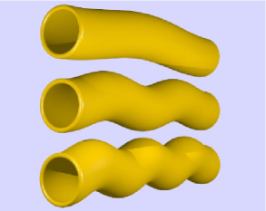
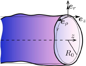
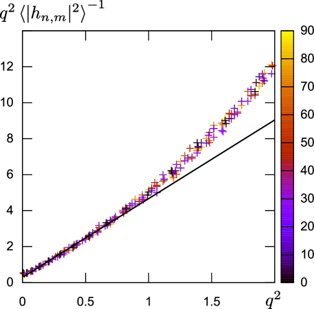
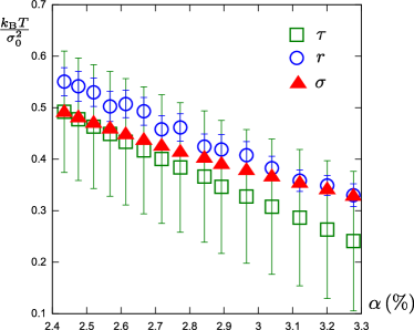
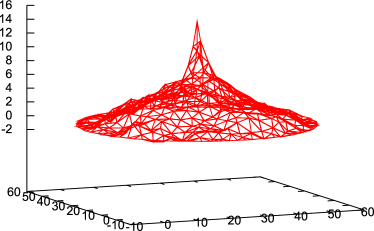
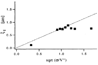
\labo

Matière et Systèmes Complexes \schoolMatière Condensée et Interfaces \specialityPhysique théorique \universityl’UNIVERSITÉ PARIS.DIDEROT (Paris7)UNIVERSITÉ PARIS.DIDEROT (Paris7) \advisor[M]Jean-Baptiste FOURNIER \coadvisor[M] \jury \jurymember[Mme]Patricia BASSEREAUPrésident du jury
\jurymember[M]Andrea PARMEGGIANIRapporteur
\jurymember[M]Dominique MOUHANNARapporteur
\jurymember[M]Laurent LIMOZINExaminateur
\jurymember[M]Alberto IMPARATOExaminateur
\juryadvisor

Forces et fluctuations en
membranes planes, sphériques et
tubulaires

Camilla BARBETTA
(07/09/2010)
\resume

Les membranes lipidiques constituent des matériaux très particuliers: d’une part, elles sont très peu résistantes aux étirements microscopiques; d’autre part elles sont extrêmement flexibles, présentant des déformations même à des petites échelles. En conséquence, une portion de membrane possède un excès d’aire relatif à l’aire optiquement visible, qu’on appelle l’aire projetée. D’un point de vue mécanique, on peut alors distinguer trois tensions associées aux membranes lipidiques: la tension mécanique effective τ𝜏\tau, associée à l’augmentation de l’aire projetée et au lissage des fluctuations; la tension σ𝜎\sigma, associée à l’aire microscopique de la membrane et donc non-mesurable, mais couramment utilisée dans les prédictions théoriques; et son équivalent macroscopique mesuré à travers du spectre des fluctuations, r𝑟r. Jusqu’au moment, pour interpréter les données expérimentales, on suppose l’égalité entre ces quantités. Dans cette thèse, nous avons étudié, en utilisant le tenseur des contraintes projeté, si et sous quelles conditions il est justifié d’assumer τ=σ𝜏𝜎\tau=\sigma. Nous avons étudié trois géométries (planaire, sphérique et cylindrique) et obtenu la relation τσσ0𝜏𝜎subscript𝜎0\tau\approx\sigma-\sigma_{0}, où σ0subscript𝜎0\sigma_{0} est une constante qui dépend seulement du plus grand vecteur d’onde de la membrane et de la température. En conséquence, nous concluons que négliger la différence entre τ𝜏\tau et σ𝜎\sigma est justifiable seulement pour des membranes sous grande tension: pour des tensions faibles, il faut considérer des corrections. Nous avons étudié les implications de ce résultat à l’interprétation des expériences d’extraction de nanotubes de membrane. En ce que concerne r𝑟r, nous questionnons une démonstration précédente de son égalité avec τ𝜏\tau. Finalement, la fluctuation des forces pour les membranes planes et pour des nanotubes de membranes a été quantifiée pour la première fois. Lipid membranes constitute very particular materials: on the one hand, they break very easily under microscopical stretching; on the other hand, they are extremely flexible, presenting deformations even at small scales. Consequently, a piece of membrane has an area excess relative to its optically resolvable area, also called projected area. From a mechanical point of view, we can thus identify three tensions associated to lipid membranes: the mechanical effective tension τ𝜏\tau, associated to an increase in the projected area and to the flattening of the fluctuations; the tension σ𝜎\sigma, associated to the microscopical area of the membrane and thus non measurable, but commonly used in theoretical predictions; and its macroscopical counterpart measured through the fluctuation spectrum, r𝑟r. Up to now, the equality between these quantities was taken for granted when analyzing experimental data. In this dissertation, we have studied, using the projected stress tensor, whether and under which conditions it is justified to assume τ=σ𝜏𝜎\tau=\sigma. We studied three geometries (planar, spherical and cylindrical) and obtained the relation τσσ0𝜏𝜎subscript𝜎0\tau\approx\sigma-\sigma_{0}, where σ0subscript𝜎0\sigma_{0} is a constant depending only on the membrane’s high frequency cutoff and on the temperature. Accordingly, we conclude that neglecting the difference between τ𝜏\tau and σ𝜎\sigma is justifiable only to membranes under large tensions: in the case of small tensions, corrections must be taken into account. We have studied the implications of this result to the interpretation of experiments involving membrane nanotubes. Regarding r𝑟r, we have questioned a former demonstration concerning its equality with τ𝜏\tau. Finally, the force fluctuation for planar membranes and membrane nanotubes was quantified for the first time.

Préambule

Les membranes biologiques sont constituées principalement par des molécules lipidiques amphiphiles, i. e., des molécules qui possèdent un groupe hydrophile et un groupe hydrophobe. Le caractère amphiphile de ces molécules donne des propriétés très particulières aux membranes lipidiques: d’une part, leur cohésion est assurée principalement par des interactions hydrophobes-hydrophiles entre les lipides et l’eau et d’autre par, la membrane présente une rigidité de courbure. Le fait que les membranes s’associent surtout par répulsion à l’eau et non par des liaisons chimiques a pour conséquence la grande mobilité de ces molécules à l’intérieur de la membrane (ce qui explique l’expression liquide bi-dimensionnel fréquemment utilisée pour désigner de membranes lipidiques) et une grande fragilité à des étirements au niveau moléculaire. Une autre conséquence est leur grande flexibilité: les membranes lipidiques sont facilement déformables, même à des échelles plus petites que celles accessibles expérimentalement. Une portion de membrane possède alors un excès d’aire relatif à l’aire optiquement discernable, qu’on appelle l’aire projetée.

Imaginons maintenant une expérience: une portion de membrane est attachée à un cadre. Une force latérale τ𝜏\tau est appliquée sur le cadre de façon à augmenter l’aire projetée de la membrane. La force τ𝜏\tau correspond à la force nécessaire pour lisser les fluctuations de la membrane. Elle est donc d’origine purement entropique et nous l’appelons alors tension mécanique effective. Expérimentalement, elle correspond à la tension appliquée à travers des micropipettes sur des vésicules, par exemple. Malheureusement, les prédictions théoriques concernent normalement la tension σ𝜎\sigma associée à l’aire microscopique de la membrane, qui n’est pas mesurable. En effet, à travers l’analyse du spectre de fluctuation des membranes, il est uniquement possible de mesurer l’équivalent macroscopique de σ𝜎\sigma, la tension r𝑟r. En conséquence, lors de l’interprétation des résultats expérimentaux, l’égalité entre ces tensions est couramment admise. Dans cette dissertation, j’ai alors examiné, sous la direction de Jean-Baptiste Fournier, si et sous quelles conditions cette hypothèse est valable pour des géométries diverses.

Dans la première partie de cette thèse, nous étudions le cas d’une pièce plane de membrane (résultats présentés dans le chapitre 2 et publiés en [1]). Dans la littérature scientifique, nous trouvons quelques relations entre τ𝜏\tau, σ𝜎\sigma et r𝑟r, sans qu’il aie un consensus [2][3]. Toutes ces dérivations, cependant, partent de l’énergie libre, ce qui peut-être très subtile, comme on discutera dans la section 2.2. Nous avons alors utilisé comme base de nos calculs le tenseur des contraintes projeté, un outil développé récemment [4] et introduit en 1.5.2, à partir duquel on a pu obtenir directement la tension τ𝜏\tau en fonction de σ𝜎\sigma:

τσσ0,similar-to-or-equals𝜏𝜎subscript𝜎0\tau\simeq\sigma-\sigma_{0}\,, (1)

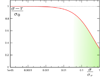
σ0subscript𝜎0\sigma_{0} est une constante qui ne dépend que de la température et du plus grand vecteur d’onde de la membrane. Ainsi, il est justifiable de considérer τσ𝜏𝜎\tau\approx\sigma seulement pour des fortes tensions. Dans ce chapitre, nous questionnons aussi une ancienne démonstration de l’égalité entre r𝑟r et τ𝜏\tau [2]: nous attendons donc en général τσr𝜏𝜎𝑟\tau\neq\sigma\neq r.

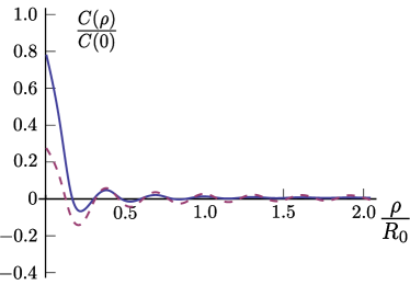
à partir du tenseur des contraintes projeté, il est aussi possible d’examiner la corrélation des contraintes sur la membrane. Ces résultats inédits sont présentés dans chapitre 3 et indiquent que ces corrélations décroissent très rapidement, indépendemment de la tension de la membrane. Les calculs développés dans ce chapitre ont été fondamentaux pour introduire et maîtriser une représentation diagrammatique des moyennes proposée par nous et inspirée des diagrammes de Feynmann. Ces outils sont repris dans le chapitre 6 et simplifient grandement les évaluations.

Expérimentalement, une pièce planaire de membrane est difficile à manipuler. Plus populairement, des vésicules de grande taille qui peuvent être manipulées avec de micropipettes sont utilisées en laboratoire. Nous avons alors étudié le cas des vésicules quasi-sphériques fermées (dont le volume interne est fixe) et percées (dont le volume n’est pas contraint) dans la partie II de cette thèse (résultats obtenus en collaboration avec Alberto Imparato et publiés sur [5]). Après avoir dérivé le tenseur des contraintes pour cette géométrie, nous concluons que la différence entre τ𝜏\tau et σ𝜎\sigma est bien approximée aussi dans le cas des vésicules sphériques (percées ou non) par la relation montré dans l’eq.(1). Une conséquence intéressante est la possibilité d’avoir une vésicule dont la pression interne est plus petite que la pression externe, ce qui est impossible pour le cas d’une goutte de liquide.

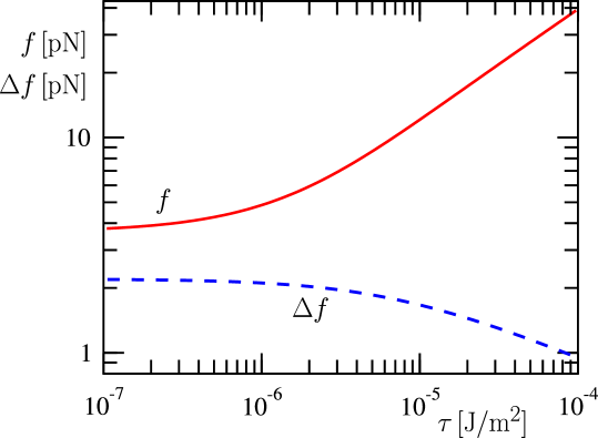
Dans la troisième partie de la thèse, nous examinons les conséquences de nos résultats pour les expériences d’extraction de nanotube de membrane (résultats publiés en [6]). Dans ces expériences, une bille en verre, par exemple, est attachée à la membrane. Avec une pince optique, une force est appliquée à la bille et un nanotube de membrane est extrait. Jusqu’au moment, ces expériences ont été interprétées en supposant la validité de deux hypothèses: la différence entre entre τ𝜏\tau et σ𝜎\sigma est négligeable et les fluctuations thermiques des tubes peuvent être également négligées. Dans ces conditions, une relation très simple relie la force appliquée par la pince optique à la tension de la membrane. Il a été cependant montré que ces fluctuations sont très importantes dû à la présence de modes très peu énergétiques [7] (modes de Goldstone). Nous avons dédié le chapitre 5 à l’étude les effets des fluctuations thermiques sur la relation entre la force et la tension de la membrane. Curieusement, nous concluons que par coïncidence, ces effets sont compensés par l’hypothèse τσ𝜏𝜎\tau\approx\sigma dans le régime de forte tension, justifiant à posteriori le traitement habituel des données expérimentales.

Avec le montage expérimental utilisé pour extraire des tubes de membrane, nous pouvons non seulement mesurer la force nécessaire pour l’extraire, mais aussi la déviation quadratique moyenne de cette force dans la direction de l’axe du tube. Cette quantité pourrait fournir des informations supplémentaires sur les caractéristiques mécaniques des membranes. Utilisant les outils diagrammatiques introduits précédemment, nous évaluons alors la déviation quadratique moyenne de la force nécessaire pour extraire un tube dans le chapitre suivant. Nous prédisons une dépendance très faible de cette quantité en fonction de la tension et de la rigidité de courbure. En conséquence, la fluctuation de la force est peu utile pour la caractérisation mécanique des membranes. Par contre, nous discutons dans ce chapitre une possible utilisation dans la caractérisation de l’activité des pompes actives insérées dans les membranes.

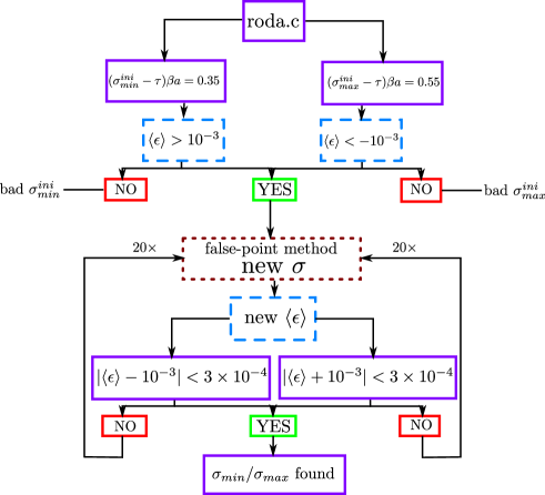
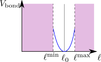
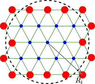
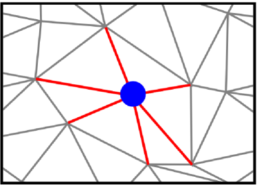
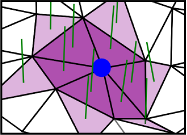
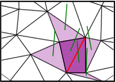
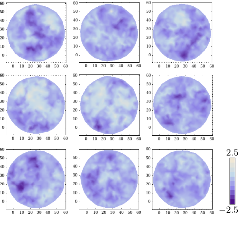
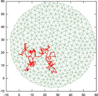
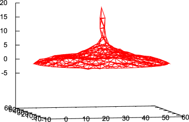
Finalement, dans la dernière partie, nous présentons les premiers résultats concernant une simulation numérique proposée par nous dans l’objectif de vérifier nos prévisions. Nous considérons une pièce planaire de membrane attachée à un cadre circulaire. La membrane a été modélisée de façon très simplifiée par des particules effectives reliées par un réseau triangulaire dont les liaisons se réarrangeaient pour assurer la liquidité de la membrane. L’objectif de cette simulation est de reproduire les conditions d’une vraie expérience: la tension τ𝜏\tau était contrôlée par la tension appliquée au cadre circulaire et le spectre de fluctuation pouvait être mesuré. En outre, dans ce cas, la tension interne σ𝜎\sigma pouvait être lié à l’extension des liens entre les particules effectives et donc estimée. Dû à des contraintes de temps, nous présentons dans ce chapitre seulement quelques résultats préliminaires.

Remerciements

Initialement, je voudrais remercier Jean-Baptiste Fournier pour m’avoir permis de faire cette thèse sur un sujet que je trouve très intérressant. J’ai beaucoup apprécié le fait que mon travail soit théorique, mais jamais très éloigné des applications/vérifications expérimentales. Merci pour m’avoir poussé à m’améliorer, surtout dans la clarté des mes textes - j’ai beaucoup râlé, mais j’ai beaucoup appris!

Je voudrais aussi remercier aux deux collaborateurs avec qui j’ai travaillé: Alberto Imparato et Luca Peliti. Vous m’avez fait sentir suffisamment à l’aise pour dire à voix haute les idées qui me traversaient la tête.

Dans la suite, je remercie à tous mes incroyables collègues de bureau et d’enseignement pour la bonne ambiance et les bons souvenirs:

  • Yann, pour sa patience toute orientale;

  • Franck, pour son attitude “no stress”;

  • Kristina, ma copine de bureau et amie. Je t’admire beaucoup!;

  • Benoit, pour tous les déjeuners et rigolades lors des goûters.

  • Damien, un français très brésilien, pour m’avoir motivé à participer à des activités très françaises - les manifestations. Merci aussi pour ton implication dans l’enseignement et dans notre petit projet pédagogique;

  • Gérald, pour les idées assez polémiques qui engendraient des grandes discussions;

  • Milad, pour sa compagnie dans notre trajet de bus;

  • Anne-Florence, pour sa bonne humeur, son talent culinaire et pour avoir arrosé mes plantes;

  • Alexandre, pour les déjeuners et cafés en langue maternelle.

Je remercie aussi tous les autres collègues que je n’ai pas eu la chance de connaître mieux, mais qui ont tous été très sympas avec moi.

J’embrasse aussi très fort le groupe fidèle d’amis que j’ai fait pendant mon master: Sophie Aimon, Fabien et Céline Paillusson, Thomas Guérin et Fanny, Laura Messio et Sébastien Boyaval. Grâce à vous je me suis sentie finalement bien intégrée ici.

Pensant au passé, un jour de ma vie a changé définitivement mon futur: le jour où j’ai passé les examens d’admission à Polytechnique. Merci aux examinateurs pour m’avoir fait confiance. Je suis très reconnaissante à la petite communauté brésilienne qui a été une deuxième famille pour moi pendant mes deux premier années en France et qui reste très soudée. Un grand merci en particulier à Ricardo Malaquias.

Je remercie ma lointaine famille pour avoir toujours donnée priorité à mon éducation et pour avoir toujours respecté mes choix. Finalement, je suis infiniment reconnaissante à la personne la plus douée et généreuse du monde, dont j’ai la chance de partager le quotidien depuis presque une dizaine d’années: Vitor Sessak.

Chapter 1 Introduction

In this section we will present membranes, first from a biological and historical point of view (section 1.1) and secondly from a modern physical perspective (section 1.2). In section 1.2.1, we define the quantities that are the focus of this work: the mechanical tension τ𝜏\tau, the Lagrange-multiplier σ𝜎\sigma and its measurable counterpart r𝑟r. The main theoretical models for membranes, as well as their validity, are presented in section 1.3. There we derive the first fundamental results for planar membranes in contact with a lipid reservoir. Section 1.4 summarizes the most current experimental techniques used to characterize the mechanics of membranes. Finally, the stress tensor for planar membranes is introduced in section 1.5.

1.1 Biological membranes

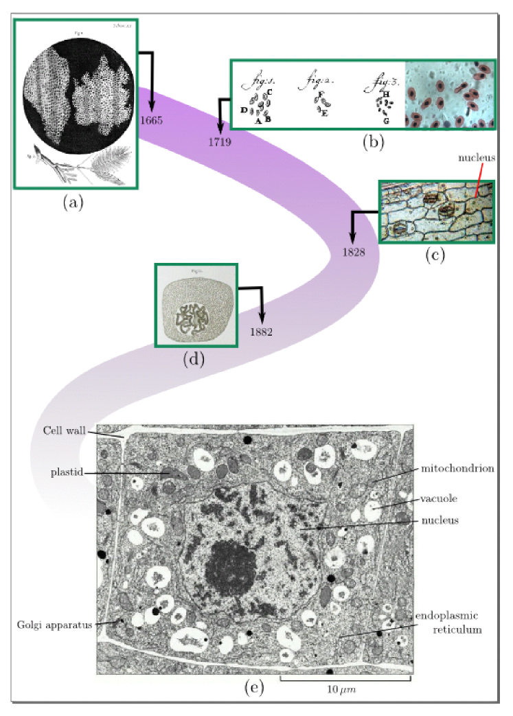
During the last four hundred years, the image of the cell has become more and more complex [8] (see Fig. 1.1). As experimental techniques evolved, many questions were answered – and many others were raised. In particular, we have learned a lot about the cell’s boundary. We will start thus by a brief non-exhaustive historical review (further details can be found on [8][9][10][11]).

Up to the 191919th century, living beings were believed to have a sponge-like microscopical structure. There would be two continuous substances: a membranous meshwork, as one can see in inset 1.1(a), and a fluid filling the communicating cells. The meshwork was considered the true essential constituent, while the fluid had a mere nourishing function [8]. At that time, the term membrane named already the cell’s boundary, although it corresponded more to what we nowadays call the cell wall, the rigid cellulose structure that encapsulates plant cells. This image changed in 1807, when Link showed that cells were in fact separated. He observed that colored fluids did not diffuse through the surrounding cells, as one would expect with the former theory. He concluded thus that the essential component of life was the unitary cell itself.

Due to the low numerical aperture of the microscopical objectives available at that time (see inset 1.1(c) for a typical image), animal cells were also believed to have a membrane, i. e., a cell wall. Cells from both animals and plants had then the same features: a nucleus, an aqueous plasma and a cell wall. This apparent universality was an important support to the cellular theory proposed by Schwann and Schleiden, which stated that every living being was constituted by cells.
Refer to caption
Figure 1.1: The cell through history. Inset (a) shows the first representation of the cell, or more precisely, of the cell walls, by Hooke in 1665. Inset (b) left shows the first drawing of the nucleus accurately made by Leeuwenhoek in 1719, while he studied the salmon red blood cells (which are nucleated in fishes). The right photo shows a contemporary optical microscope image of the same cells for comparison. The next inset shows a modern photograph of plant tissue taken with roughly the same technology as in 1828, five years before Brown, best known for his observations of the Brownian motion, named the nucleus. Inset (d) depicts the chromosomes inside the nucleus (Flemming). Finally, sub-figure (e) shows a nowadays electron micrography of a plant cell [12]. We can see the complicated internal structure and identify some organelles.

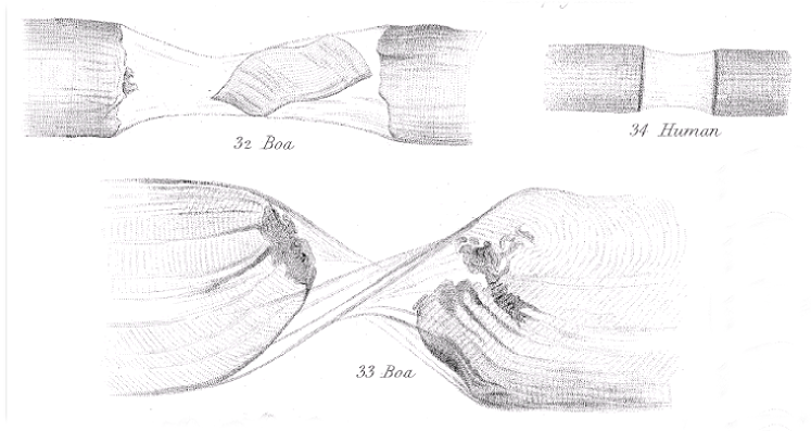
Some years later, the histologist and physiologist William Bowman [13], best known for his work in nephrology (the Bowman’s capsule is named after him), represented for the first time an actual cell membrane. In his 1840 work, he studied the striated muscle cells [14]. He noticed that by stretching those cells, he could disrupt their internal fibers leaving a transparent sheath called sarcolemma intact (see Fig. 1.2). This sheath, in that time thought a cell wall, is actually what we currently call the cell membrane.

Subsequent experiments on the effects of osmotic pressure on plant cells showed that the cell could pull away from the cell wall. This phenomenon is called plasmolysis. It is caused by the selective permittivity of the cell membrane, which is permeable to water, but not to ions, sugars and other water soluble molecules. Although specialist of that time could have interpreted it as an indirect evidence of a membrane encapsulating the cell, they blamed osmotic effects on vacuoles and proposed the naked-cell theory: the cell was defined as a small naked lump of protoplasm with nucleus, in Schultze’s words (1860). It could eventually be encapsulated by a non-essential skin (de Bary, 1861) [8].
Refer to caption
Figure 1.2: Drawings from Bowman’s work representing boa and human striated muscle cells [14]. The disrupted fibers are enclosed by a sheath called sarcolemma: the cell membrane.

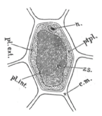
The first one to realize that there was effectively a skin of different nature around the protoplasm was Ernest Overton in 1895 [15]. He noticed that plant cells under a 8%percent88\% sugar solution suffered plasmolysis. This indicated that sugar molecules could not easily penetrate the cell even though the protoplasm was composed by water. He repeated the experiment using successive solutions of alcohols, ether, acetone and phenol with the same osmotic pressure as the sugar solution. He remarked that in some of these cases there was no plasmolysis, depending on the substance solubility in water. He concluded that water insoluble substances penetrated easily the external part of the protoplasm (Grenzschicht), whereas water soluble molecules, as sugar, did not. He inferred thus that the boundary region was distinct from the rest of the protoplasm (see Fig. 1.3) and that it was impregnated by a substance of the same nature of fatty oils.

Indeed, today we know that biological membranes are mostly composed by amphiphilic lipids, having a hydrophobic tail and a hydrophilic head. This feature make them self-assembly in aqueous media in large bilayers, even though there are no chemical bonds between them. This explains the relative impermeability of membranes to water soluble substances. The most abundant kind of lipid present on membranes are phospholipids. These molecules have one or two long hydrocarbon chains, which may contain only simple bonds (saturated) or double bonds (unsaturated). As we shall see in section 1.2, the stability of the bilayer is assured by the fact that these molecules have an effective shape close to a cylinder, whose dimensions are typically 0.5nm0.5nm0.5\,\mathrm{nm} for the radius and 1.01.5nm1.01.5nm1.0-1.5\,\mathrm{nm} for the length [16]. In addition to phospholipids, membranes may also contain cholesterol, an amphiphilic lipid that unlike phospholipids has a ring-like tail.
Refer to caption
Figure 1.3: Schematic representation of a plant-cell made by Overton in his 1895 work [15]. The cell wall (indicated by c.m.) and the cell membrane (indicated by pl.ext.) are represented as different entities. Note that Overton decided arbitrarily the thickness of the membrane.

The first indirect estimation of the membrane thickness was made by Hugo Fricke in 1925. He measured the capacitance of blood cells and, supposing that they were composed by lipids, deduced a thickness of 3.3nm3.3nm3.3\,\mathrm{nm} [17]. This is a remarkable result, since posterior direct measures give a thickness between 5nm5nm5\,\mathrm{nm} and 10nm10nm10\,\mathrm{nm} [18]. Meanwhile, Gorter and Grendel gave a fundamental step towards the comprehension of how lipids arrange themselves within the membrane [19]. They extracted the lipids from a known number of red blood cells. Using a Langmuir trough, they measured the area covered by lipids and it corresponded to twice the estimated surface area of the erythrocytes. They deduced that the membrane was constituted by a bilayer of lipids whose polar heads pointed outward.

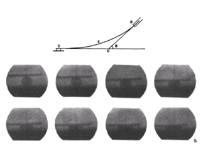
In 1932, a puzzling experiment suggested that there was more than lipids on a membrane. Kenneth Cole studied urchin eggs by compressing them between a plate and a gold fiber with a known force, much in the same way as in modern experiments [20] (see Fig. 1.4). He deduced the tension of the egg’s membrane by studying its degree of flattening. His measures yielded a tension of 0.08dyn/cm0.08dyncm0.08\,\mathrm{dyn}/\mathrm{cm}, which is a hundred times smaller than the tension of oily films [21]. This was a surprising result, if one believed the membrane to be constituted only by lipids.
Refer to caption
Figure 1.4: Original drawing and photos from Cole’s experiment on urchin eggs: the egg (D) is compressed by a gold fiber (E).

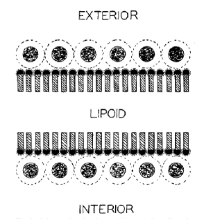
Two years later, Danielli and Harvey solved the paradox. They centrifugated smashed mackerel eggs in order to separate lipids from the aqueous phase. First, they measured the surface tension of the oily phase and obtained 9dyn/cmabsent9dyncm\approx 9\,\mathrm{dyn}/\mathrm{cm}. Then they added the aqueous phase and observed a tension lowering. By studying the time evolution and the influence of temperature on their mixture, they deduced that proteins were responsible for the tension lowering [22]. Danielli and Davson proposed in the following year the first model of the membrane structure: every plasma membrane would have a core of lipids bordered by two monolayers of lipids whose polar head pointed outward and the whole would be coated by a layer of proteins [23] (see Fig. 1.5). It was an important step, since today we know that proteins are responsible for almost every membrane function but enclosing, such as active transport of molecules, binding to cytoskeleton and reception of chemical signals from the outer environment.
Refer to caption
Figure 1.5: Original drawing from Danielli-Davson’s paper representing the membrane structure: a bulk of lipids bordered by ordered lipid monolayers covered with proteins.

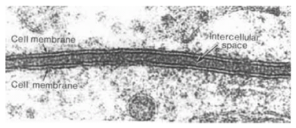
In the 1950s the new technology of electron micrography allowed to make the first direct images of the cell membrane (see Fig. 1.6). The use of permanganate fixation was also important, since it stained only the hydrophilic head of lipids. Robertson observed a three line pattern of about 7.5nm7.5nm7.5\,\mathrm{nm} corresponding to a simple bilayer. This excluded the possibility of a bulk of lipids in membranes. He observed the three lines pattern not only on the cell boundary, but also encapsulating organelles from different animals and bacteria [18]. Moreover, using innovative staining processes, he showed the asymmetry of some membranes’ coating, the external surface containing also carbohydrates. These new features were incorporated in the unit membrane model: every biological membrane shared the same architecture - a lipid bilayer, asymmetrically coated by proteins and carbohydrates.
Refer to caption
Figure 1.6: Electron micrography of the cell membrane [24]. The hydrophilic heads of lipids are colored, while the hydrophobic tails are not. This results on the characteristic three lines pattern seen above.

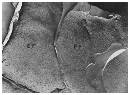
Some years later, the advent of the freeze fracture etch (FFE) electron microscopy brought new advances. This technique consists on freezing cells by immersion on nitrogen. The block of cells is then fractured. By deposing carbon and platinum vapor, a replica of the fractured surface is constituted. At last, the replica can be examined by a transmission electron microscope. In the late 1960s, da Silva and Branton showed that on biological membranes, these fractures tended to pull apart the lipid bilayer [25][26]. They obtained the micrography shown in Fig. 1.7(a), which suggested that proteins were actually embedded in the lipid bilayer. Besides, another work using fluorescent labeling showed that proteins diffuse, implying that membranes were in fact fluid [27] (see Fig. 1.7(b)).
Refer to caption
(a) Micrography of a fractured human erythrocyte membrane. The left surface corresponds to the external fracture (EF) and the right corresponds to the protoplasmic fracture (PF). The tiny particles on both surfaces measure between 555 and 10nm10nm10\,\mathrm{nm} and correspond to proteins. Note that they are more numerous on the PF face due to the presence of peripheral proteins attaching the membrane to the cytoskeleton.
Refer to caption
(b) Original picture of the fluorescence labeled antigens experiment which showed that proteins diffuse on the cell membrane[27]. Antigens were labeled in red (lower half) and green (upper half). After some minutes, the colors were uniformly distributed over the cell.
Figure 1.7: Evidences in favor of the Mosaic Fluid model.

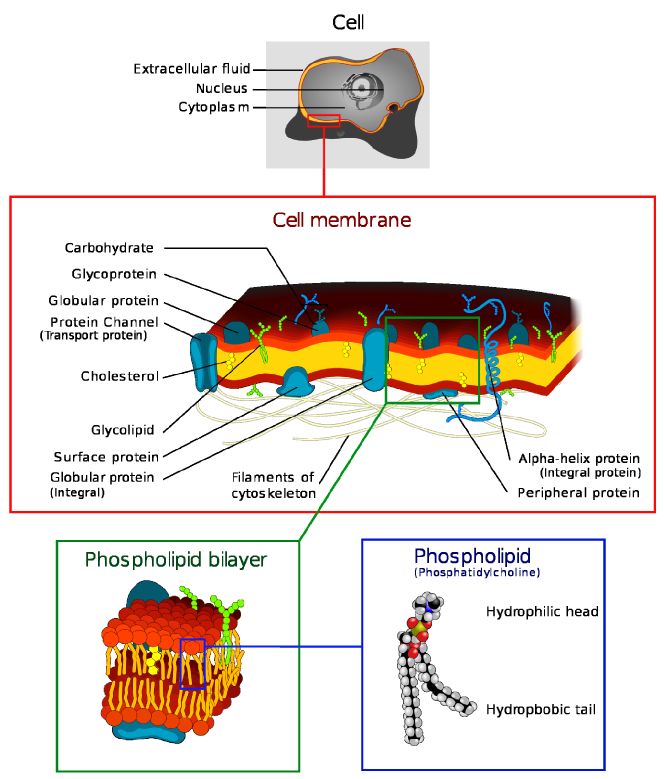
Finally, bearing in mind these experiments, Singer and Nicholson proposed the mosaic fluid model of membranes (see Fig. 1.8 for a sum-up), which is the basis to the modern vision of biological membranes. They made the distinction between peripheral proteins, i. e., those loosely attached to the membrane like those that bind the membrane to the cytoskeleton, and the integral proteins, which are embedded in the lipid bilayer. They postulated that lipids and proteins diffuse freely inside the membrane’s surface, as a two-dimensional liquid. Consequently, membranes should have no long-range order. They noted that the membrane leaflets were probably asymmetrical with respect to lipid and protein composition due to the energy barrier of moving the polar head from the aqueous interface into the bilayer interior. Later experiments confirmed that asymmetry was indeed present on biological membranes [28].
Refer to caption
Figure 1.8: Schematic view of a biological membrane as proposed by the fluid mosaic model. The green inset shows the bilayer structure in detail and the blue inset represents of a phospholipid (phosphatidylcholine), also known as lecithin, present in egg yolk. Remark the unsaturated bond in one of its tails.

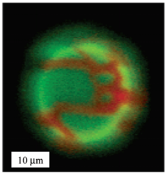
The model was elegant, but experiments rapidly showed that it was oversimplified. Biological membranes are not so homogeneous as the fluid mosaic model implies. Already in the 808080’s, indirect measures showed that polarized epithelial cells present membrane domains, i. e., the cell membrane that faces a cavity has different composition from the other faces [29]. Moreover, biological membranes present also smaller domains, ranging from dozens to hundreds of nanometers [30]. A simple statistical reasoning suggests that heterogeneities should indeed be expected: a random lipid and protein distribution means that the pairwise interactions between lipid-lipid, lipid-protein and protein-protein should be within thermal energies, which is rather improbable, given their wide variety [31].
Refer to caption
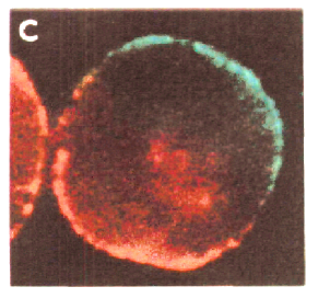
(a) Photo of a vesicle composed by a 1:1:111:1 mixture of DLPC and DPPC, two kind of phospholipids. The green and red patches represent respectively the fluid and the gel phase.
Refer to caption
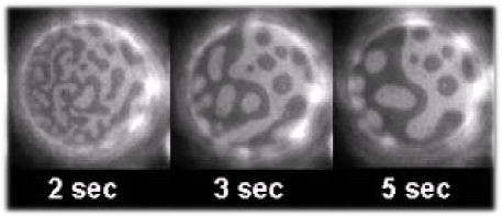
(b) Time evolution of a vesicle composed by a 1:1:111:1 DOPC and DPPC (phospholipids) mixture added of 35%percent3535\% cholesterol. We see also a phase separation, but this time both phases are liquid. Remark the domains widen with time.
Figure 1.9: Phase separation on membranes.

At this point, model membranes, i.e., lipid bilayers reconstituted in laboratory to mimic biological membranes (see section 1.2), confirmed and gave new insight to the question of lipid phase separation. A mixture of phospholipids in the gel/liquid phases segregates, as shown in Fig. 1.9(a) [32]. At the interface between these phases, a line tension builds up and they tend to separate in order to minimize energy. More interestingly regarding cells, it is possible to have phase separation between two liquid phases: the liquid-disordered and the liquid-ordered [16]. Experimentally, this may be achieved in a mixture of phospholipid and cholesterol [33][34] (see Fig. 1.9(b)).

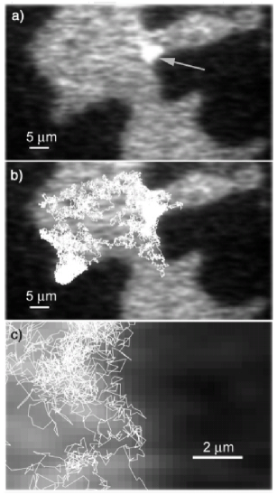
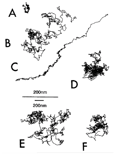
Besides the segregation of lipids, it was also shown that some proteins cluster in model membranes. In these cases, the aggregation depends on the length of the lipids constituting the bilayer where proteins are embedded [35]. In addition, modern techniques, such as single particle tracking, show that lipids and proteins in living cells can have anomalous movements, such as directed or confined motion and anomalous diffusion, possibly due to the cytoskeleton or to restrictions imposed by lipid domains [36] (see Fig. 1.10).
Refer to caption
(a) typical trajectories of gold particles attached to certain proteins on a cell surface (followed for 30s30s30\,\mathrm{s}). Trajectory A corresponds to the stationary mode, B, E and F to simple diffusion, C to directed diffusion and D to restricted diffusion [37].
Refer to caption
(b) Here, single particle tracking is used to study a model lipid monolayer divided in two phases: the liquid-ordered (dark gray) and liquid-disordered (light gray). The arrow in (a) indicates the polystyrene bead that was tracked. Fig.(b) shows the bead’s random walk and (c) shows a detail of this walk. Remark that the bead remains on the liquid-disordered phase [38].
Figure 1.10: Single particle tracking.

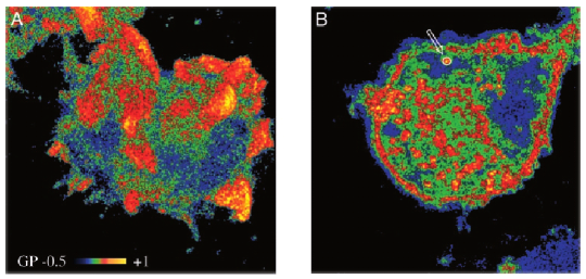
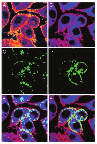
Finally, modern fluorescence techniques allow the direct visualization of domains in living cells [39]. In Fig. 1.11, Fig. 1.12.A and Fig. 1.12.B, one can see patches whose overall structure is different. The discriminating feature is the GP (generalized polarization): red for liquid-ordered phase, richer in cholesterol, and blue the liquid-disordered phase. The images show clearly that there is coexistence of liquid phases in cells. Moreover, it is possible to detect certain types of proteins. In Fig. 1.12.C and in Fig. 1.12.D, transferrin receptor and caveolin-1 are respectively shown by fluorescence. Fig. 1.12.E and Fig. 1.12.F show the merge of C and D with B, respectively. We can see that the transferrin receptor is found mostly on the liquid-disordered phase, while caveolin-1 is found mostly on the liquid-ordered phase. Indeed, for a long time liquid structures called rafts composed mostly by glycosphingolipids, cholesterol and some proteins were suspected to exist [16]. These rafts would help protein sorting and be involved in cell signaling. These images present however only some evidence of their existence and the subject is still debated [40][41].

Refer to caption
Figure 1.11: GP images of living macrophages (mouse RAW264.7𝑅𝐴𝑊264.7RAW264.7 and human THP1𝑇𝐻𝑃1THP-1, respectively): red stands for the liquid-ordered phase and blue to the liquid-disordered. The circled area indicated in B shows the pixilation of the image (167167167 pixels inside the circle). Note in A that liquid-ordered phase tend to be observed on the tip of filopodia [39].
Refer to caption
Figure 1.12: Images of RAW264.7𝑅𝐴𝑊264.7RAW264.7 living cells. Figure A shows the GP image and B shows the corresponding dual-colored image. Figs.C and D show the fluorescence images for transferrin receptor and caveolin-1, respectively. Figs.E and F correspond to the superposition of B with C and D, respectively: light blue patches indicate colocalization with liquid-disordered phases and yellow patches indicates colocalization with liquid-ordered phases[39].

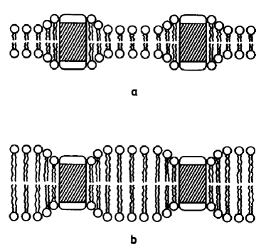
In order to account for some of these results, refinements of the fluid mosaic model were proposed. For instance, to explain protein clustering Mouritsen proposed the Mattress Model [42] (see Fig. 1.13). The model comes from the observation that the bilayer thickness may be smaller or larger than the length of the hydrophobic part of embedded protein. This mismatch would expose hydrophobic parts of the protein or of the lipids, which would in consequence deform. The deformation would give rise to a line tension which would tend to cluster proteins and aggregate some kinds of lipids. Another model was proposed by Erich Sackmann to explain the confinement of proteins observed during single particle tracking. It stresses the interactions between the membrane and the cytoskeleton. To the moment however, there is no model that accommodates all recent results about biological membranes.
Refer to caption
Figure 1.13: Drawing representing the Mattress model: hydrophobic mismatch deforms lipids. Proteins tend thus to aggregate.

1.2 Model membranes and mechanical probing

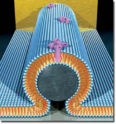
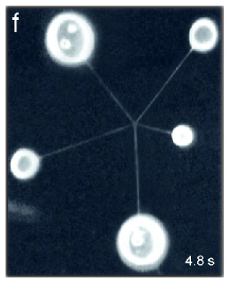
As we have seen in the last section, biological membranes are very complex. Simpler membranes reconstituted in laboratory called model membranes are thus doubly interesting. First, they give insight to the comprehension of phenomena in living cells. Model membranes are advantageous because they have both chemical composition and environment controlled, allowing reproducible experiments. Moreover, these membranes are generally in thermodynamic equilibrium, which is impossible to achieve in living cells. By consequence, these experiments may be described using conventional statistical mechanics tools. Secondly, model membranes have technological interest in their own: they are used to improve drug delivery, to build micro-chambers for chemical reactions [43][44] and even to build bio-electronic devices [45] (see Fig. 1.14).
Refer to caption
(a) Fluorescence micrography of a self-tightened knot (center of image) made of lipid nanotubes extracted from membrane vesicles. The vesicle on the left is about 10μm10𝜇m10\,\mathrm{\mu m} [44].
Refer to caption
(b) Artistic representation of a bio-electronic device composed by a nanowire 30nm30nm30\,\mathrm{nm} wide (gray) covered by a lipid membrane (blue/orange). In this membrane, proteins that control ion passage were incorporated (pink) (image by Scott Dougherty, [45]).
Figure 1.14: Technological applications of membranes.

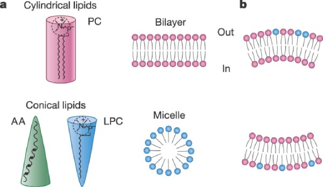
Model membranes are prepared by dissolving phospholipids in an aqueous solution. In order to minimize the exposition of their hydrophobic tails to water, they self-assemble in a large variety of forms, from small micelles to vesicles and bilayers, depending on temperature, on concentration and on the effective shape of phospholipids, which is a measure of their average cross section of as a function of how profoundly buried they are on a membrane. In Fig. 1.15(a), we can see examples of effective shapes. Note that to form a bilayer, lipids must have roughly a cylindrical shape. In Fig. 1.15(b), we can see an asymmetrical bilayer, which naturally tends to bend. We remark that the leaflets’ asymmetry is stable over time, since spontaneous passage of lipids from one monolayer to the other, known as flip-flop, is very slow in pure lipid bilayers (of the order of several hours [46]). Indeed, there is a high energetic barrier for the hydrophilic head to traverse the hydrophobic core of the membrane.

An essential point is the very weak water solubility of phospholipids. This implies that once a structure such as a vesicle is formed, the number of phospholipids it contains is constant. Besides, phospholipids do not resist to stretching, as we will see in section 1.2.1 and thus the total area of these structures is also constant.
Refer to caption
Figure 1.15: Inset (a) shows the effective shape of some phospholipids: in pink, phosphatidylcholine (PC), in blue lysophosphatidylcholine (LPC), with only one hydrophobic tail, and in green arachidonic acid (AA), with an unsaturated tail. The upper surface corresponds to the hydrophilic head. In the center, we can see some self-assembled structures. Inset (b) shows an asymmetrical bilayer whose composition leads to a natural bending tendency.

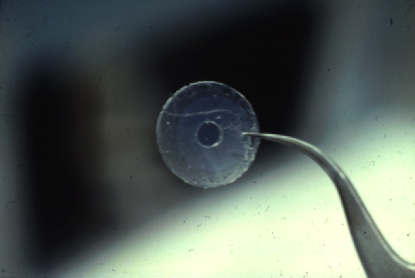
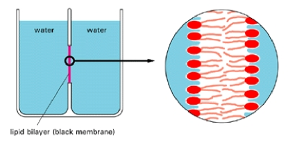
In this work, we are interested in the mechanical properties of liquid membranes. To this aim, three structures are usually studied: planar membranes, vesicles and membrane tubes. Planar membranes are also called black film membranes (BLM). They are used since the 606060’s and their name come from the destructive interference that a light beam suffers due to the thinness of the lipid membrane. The experimental set is constituted by two aqueous chambers separated by a plate (see Fig. 1.16(a)). This plate, usually made of hydrophobic materials to assure the adherence of lipid molecules, has a hole ranging from micrometers to several millimeters (see Fig. 1.16(b)). A bilayer can be deposed over this aperture through a variety of techniques [47]. BLMs are widely used to characterize the electrical properties of membrane spanning proteins, since one can control the composition of both aqueous solutions. It has also been used in single particle tracking [48].

Sadly, the technique presents many disadvantages for mechanical probing. First, one cannot control the tension of the frame: it depends on the film deposition. If the tension is too small, the membrane fluctuates a lot and is unstable. So, usually the film is relatively tense. If however it is too tense, a minimum osmotic difference between the two cavities leads to the rupture of the membrane [49]. Another problem is the film deposition technique, which may involve solvents that contaminate the membrane [50].
Refer to caption
(a) Drawing of the experimental set used in black film experiments.
Refer to caption
(b) Photo of the Teflon foil used to separate the two chambers shown above. The hole is about 1mm1mm1\,\mathrm{mm} large. The lipid membrane is deposed over this aperture [51].
Figure 1.16: Black lipid films.

The most popular objects used for membrane mechanical probing are uni-lamellar vesicles, which are self-assembled bags of a single bilayer containing fluid. They are obtained from several techniques and range in size from a few tens of nanometers to tens of micrometers. In the last case, they are also called GUV (giant uni-lamellar vesicles) and they are of special interest, since they have roughly the same size of cells, they are easy to manipulate and they are directly visible with light microscopy techniques [52]. Moreover, they are stable and they can be deflated by changing the osmotic pressure. Each vesicle has a constant surface, since phospholipids are weakly soluble in water and their volume is also constant, as long as the osmotic pressure is kept constant.

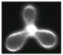
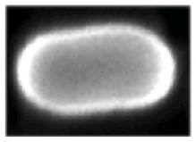
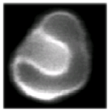
They appear in a variety of fluctuating shapes (see Fig. 1.17), whose average form depends on the enclosed volume, total area and the asymmetry between the leaflets that form the bilayer [16][53]. Note however that these images are coarse-grained, as the wave length of light, about half a micron, is much bigger than the membrane thickness. So, only low-frequency fluctuations are visible.
Refer to caption
Refer to caption
Refer to caption
Figure 1.17: Prolate, stomatocyte and starfish vesicles made of a ternary mixture of phospholipids and cholesterol [54]. The high frequency deformations are not optically resolvable.

In the last ten years, another structure used to characterize a membrane are membrane nanotubes, such as those seen of Fig. 1.14(a). These tubes are formed when a point force is applied to a lipid bilayer. Their radii range from a few to hundreds of nanometers. We will discuss them in detail in section 1.4.4.

1.2.1 How do you characterize mechanically a membrane?

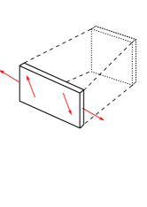
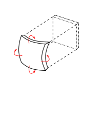
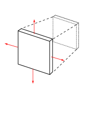
The first way to characterize the mechanical behavior of a material is by studying how it behaves under a reversible deformation, i. e., by studying its elastic deformations. On a mesoscopic scale, i. e., on length scales bigger than the material thickness, but smaller than the persistence length, which we will define in the following, one can imagine three of these deformations: bending, stretching and shearing. For thin interfaces, such as lipid membranes, bending means changing the curvature of a piece of material keeping its area constant (see Fig. 1.18), stretching means increasing the average area per molecule that composes the material by applying a tangential stress (Fig. 1.18) and shearing means changing the shape without changing its area (Fig. 1.18). As lipid membranes are composed by two leaflets, one should also consider the friction between these layers. In the following, we will deal only with static measures, so friction will not be important.
Refer to caption
Refer to caption
Refer to caption
Figure 1.18: Three mesoscopic elastic deformations used to characterize a thin interface: bending, stretching and shearing.

In liquid interfaces, such as membranes in the liquid state, molecules are free to move. Consequently, there is no resistance to shearing and we will not study this kind of deformation. The resistance to stretching is measured by the compression modulus K𝐾K. It is defined by the amount of energy EKsubscript𝐸𝐾E_{K} per unit area needed to increase a piece of surface A0subscript𝐴0A_{0} of ΔAΔ𝐴\Delta A:

EK=K2(ΔAA0)2.subscript𝐸𝐾𝐾2superscriptΔ𝐴subscript𝐴02E_{K}=\frac{K}{2}\left(\frac{\Delta A}{A_{0}}\right)^{2}\,. (1.1)

Similarly, the capacity of bending is measured by the bending rigidity modulus κ𝜅\kappa and the Gaussian curvature modulus κGsubscript𝜅𝐺\kappa_{G} defined by

Ecurv=Eκ+EκG=2κ(HH0)2+κGR1R2,subscript𝐸curvsubscript𝐸𝜅subscript𝐸subscript𝜅𝐺2𝜅superscript𝐻subscript𝐻02subscript𝜅𝐺subscript𝑅1subscript𝑅2E_{\mathrm{curv}}=E_{\kappa}+E_{\kappa_{G}}=2\kappa\left(H-H_{0}\right)^{2}+\frac{\kappa_{G}}{R_{1}R_{2}}\,, (1.2)

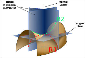
where Ecurvsubscript𝐸curvE_{\mathrm{curv}} is the energy per unit area needed to bend, R1subscript𝑅1R_{1} and R2subscript𝑅2R_{2} are the two principal curvature radii seen on Fig. 1.19, H𝐻H is the mean curvature, given by

H=12(1R1+1R2),𝐻121subscript𝑅11subscript𝑅2H=\frac{1}{2}\left(\frac{1}{R_{1}}+\frac{1}{R_{2}}\right)\,, (1.3)

and H0subscript𝐻0H_{0} is the spontaneous mean curvature. Due to the liquidity, the spontaneous mean radius R0subscript𝑅0R_{0} is isotropic and H0=1/R0subscript𝐻01subscript𝑅0H_{0}=1/R_{0}.

Refer to caption
Figure 1.19: Drawing representing the principal curvature radii of a surface.

Equivalently, the bending rigidity of a material is reflected by its persistence length ξ𝜉\xi, defined as the length beyond which the correlation in the direction of the tangent to the surface is lost. For a free membrane, it relates to the bending modulus through

ξaexp(cκkBT),𝜉𝑎𝑐𝜅subscript𝑘B𝑇\xi\approx a\,\exp\left(\frac{c\,\kappa}{k_{\mathrm{B}}T}\right)\,, (1.4)

where a𝑎a is a molecular length of the same order of the lipid’s length, c𝑐c is a constant, kBsubscript𝑘Bk_{\mathrm{B}} is the Boltzmann constant and T𝑇T is the temperature.

As a consequence of the Gauss-Bonnet theorem, the total contribution of the Gaussian curvature for closed surfaces is constant:

EκGtot=κGS1R1R2𝑑A=4πκG(1g),subscriptsuperscript𝐸totsubscript𝜅𝐺subscript𝜅𝐺subscriptcontour-integral𝑆1subscript𝑅1subscript𝑅2differential-d𝐴4𝜋subscript𝜅𝐺1𝑔E^{\mathrm{tot}}_{\kappa_{G}}=\kappa_{G}\oint_{S}\frac{1}{R_{1}R_{2}}\,dA=4\pi\kappa_{G}(1-g)\,, (1.5)

where the integral runs over a closed surface S𝑆S and g𝑔g is the genus number, which describes the topology of the surface. As we will not consider topology changes in this work, we will not consider this contribution to the energy of closed membranes henceforth.

Now, let’s see the figures for a typical phospholipid membrane. We will describe in section 1.4 how these quantities are measured. First, membranes are extremely flexible, with κ20kBT𝜅20subscript𝑘B𝑇\kappa\approx 20\,k_{\mathrm{B}}T [55], which is about a quarter of million smaller than the bending rigidity of a sheet of polystyrene of the same thickness. This implies that they fluctuate a lot even in small scales, as it has indeed been measured through NMR and X-rays techniques on stacks of bilayers [56]. Secondly, they have a high compressibility modulus K240mN/m𝐾240mNmK\approx 240\,\mathrm{mN/m} [55], which means that the stretching due to thermal fluctuation is 108%similar-toabsentpercentsuperscript108\sim 10^{-8}\,\% and thus negligible. Measures indicate that membranes rupture under a charge of only τrup10mN/msubscript𝜏rup10mNm\tau_{\mathrm{rup}}\approx 10\,\mathrm{mN/m} [55], which means that it can only stretch about 4%percent44\% before breaking apart. Indeed, as phospholipids are bonded to each other only by entropic forces and not by chemical bonds, it is relatively easy to break cohesion. Therefore, under a stress smaller than the rupture charge, it is a good approximation to consider the total area of the membrane constant, as we have discussed in last section. Throughout this work, unless explicitly said, we shall place ourselves under this condition and thus only the bending energy will be considered.

The great flexibility of membranes has an important experimental consequence: one cannot measure the true surface of a bilayer. Indeed, up to the moment, we are not able to control exactly the number of phospholipids within a membrane. Moreover, they fluctuate on a nanometric scale, not resolvable with optical microscopy techniques. Thus, it is useful to define two macroscopic quantities: the excess area and the effective or entropic mechanical tension.

The excess area α𝛼\alpha is simply a measure of the average membrane crumpling which is not optically resolvable. It is defined by

α=AApAp,𝛼delimited-⟨⟩𝐴subscript𝐴𝑝subscript𝐴𝑝\alpha=\frac{\langle A\rangle-A_{p}}{A_{p}}\,, (1.6)

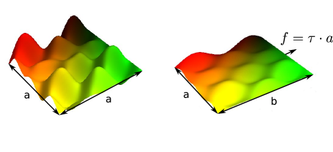
where A𝐴A is the microscopic membrane area and Apsubscript𝐴𝑝A_{p} is the optically resolvable area, which we will also call in the following the projected area (see Fig. 1.20). Experimentally, we have access only to variations on the excess area.
Refer to caption
Figure 1.20: On the left we see an illustration of the undulating surface of a membrane. The membrane area A𝐴A corresponds to the surface area of the colored membrane, while the macroscopically resolvable projected area Apsubscript𝐴𝑝A_{p} is a2superscript𝑎2a^{2}. On the right, we see an illustration of the diminution of the excess area due to a mechanical tension applied on the same membrane patch: the area A𝐴A remains the same, but the projected area is now ab𝑎𝑏a\cdot b.

The entropic mechanical tension τ𝜏\tau is a measurable macroscopic averaged tension associated to the diminution of the excess area, i.e., to the flattening of fluctuations. It is a pure entropic force, arising from the diminution of accessible configurations. It is defined as

τ=(Ap)Np,𝜏subscriptsubscript𝐴𝑝subscript𝑁𝑝\tau=\left(\frac{\partial\mathcal{F}}{\partial A_{p}}\right)_{N_{p}}\,, (1.7)

where =kBTln(𝒵)subscript𝑘B𝑇𝒵\mathcal{F}=-k_{\mathrm{B}}T\ln(\mathcal{Z}) is the free-energy of the membrane, 𝒵𝒵\mathcal{Z} is the partition function and the symbol Npsubscript𝑁𝑝N_{p} indicates that the derivative is taken under the condition that the total number of lipids is constant. In the following, as we shall consider tensions a lot weaker than the rupture tension, it is justified to consider that the total mechanical tension corresponds simply to τ𝜏\tau.

1.2.2 How different are membranes from liquid interfaces?

The aim of this section is to highlight the differences between membranes and other macroscopic materials. First, it is easy to understand why membranes behave differently from solid membranes, such as rubber membranes, since molecules of the later are not free to move. The difference is much subtler with liquid interfaces. Indeed, both present two-dimensional disorder, high deformability, form thin films (see Fig. 1.21) and in both cases the term surface tension is currently used in the literature. We shall see, however, that this expression has a different meaning in each context and that liquid interfaces are fundamentally different from membranes.

The surface tension γ𝛾\gamma on liquids is a constant of the material, depending only on the molecular composition and on temperature. At microscopical level, molecules of liquids, such as water, are strongly chemically bonded to each other and these bonds are energetically favorable. Molecules on the surface have less neighbors and are thus energetically costly: the surface tension tends to make the interface as small as possible, which results in a certain interfacial stiffness.

Refer to caption
Figure 1.21: Photo taken by International Space Station Science Officer Don Pettit of a pure water film held by a metal loop under micro-gravity. Food coloring was added only for visualizing [57]. We just do not observe this phenomenon in everyday life due to gravity.

In terms of free-energy \mathcal{F}, the surface tension is conjugated to the total area of the interface:

γ=(A)V,𝛾subscript𝐴𝑉\gamma=\left(\frac{\partial\mathcal{F}}{\partial A}\right)_{V}\,, (1.8)

where V𝑉V indicates that the derivative is taken at constant volume.

In lipid membranes, however, if there is no stretching, there is no contribution to the free-energy coming from the interface area. So, γ0𝛾0\gamma\rightarrow 0: the lipids will form a bilayer without a bulk of lipids. A noteworthy confusion in literature arises from misleadingly calling the mechanical tension τ𝜏\tau also surface tension. The tension τ𝜏\tau is also associated to a surface, but to the surface of the projected area. Moreover, it is not a material constant since it has an entropic origin. In the following, we will avoid the use of the ambiguous expression surface tension.

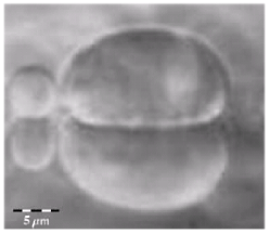
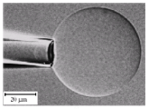
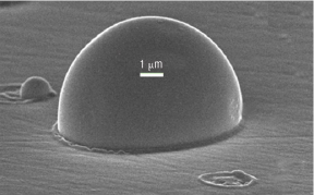
Finally, another obvious difference is the bending rigidity. Lipids in a membrane are arranged in a particular ordered way due to the amphiphilic nature of lipids, which leads to a bending rigidity. In liquids, it is not the case. We can see a consequence in Fig. 1.22: while liquid drops present a sharp contact with a substrate, membrane vesicles have a rounded contact region. Besides, one cannot expect to extract tubes by applying point forces to liquid films, as one does in membranes (see section 1.4.4).
Refer to caption
(a) Metallic liquid drop over a solid substrate. Note the sharp edges at the contact between the drop and the solid [58].
Refer to caption
(b) An optical micrography of two vesicles adhering to a pure glass substrate, which reflects the vesicles [59]. The rounded shape of the vesicle near to the glass is due to the bending rigidity.
Figure 1.22: Effect of the bending rigidity.

1.3 A model for model membranes

Here we present the three main theoretical models for liquid lipid bilayers. They describe membranes in a length scale much larger than the membrane thickness, so that it can be seen as a mathematical surface. They differ mainly in the description of the membrane’s two-leaflet structure [60]. In the following three descriptions, the microscopic area A𝐴A is kept constant. In the case of vesicles, there is an additional constraint on the volume enclosed by the surface.

1.3.1 Spontaneous curvature (SC) model

This model was introduced by Helfrich is 1973 [61] and is the very simplest one. The membrane is seen as an infinitely thin surface and its internal bilayer structure is described by a spontaneous mean curvature H0subscript𝐻0H_{0}. The Hamiltonian of a bilayer is simply given by the bending energy Ecurvsubscript𝐸curvE_{\mathrm{curv}}

SC=S[2κ(HH0)2+κGR1R2]𝑑A,subscriptSCsubscript𝑆delimited-[]2𝜅superscript𝐻subscript𝐻02subscript𝜅𝐺subscript𝑅1subscript𝑅2differential-d𝐴\mathcal{H}_{\mathrm{SC}}=\int_{S}\left[2\kappa(H-H_{0})^{2}+\frac{\kappa_{G}}{R_{1}R_{2}}\right]\,dA\,, (1.9)

where the integral runs over the membrane surface S𝑆S.

1.3.2 Bilayer couple (BC) model

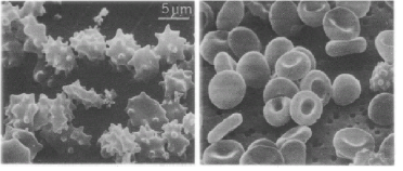
In this model, the two leaflets of a bilayer may respond differently to an external perturbation, such as chemical substances, while remaining coupled [62]. It was first introduced in 1974 to explain qualitatively experiments on red blood cells [63][64]. It had been observed that erythrocytes treated with amphiphilic drugs change of shape, becoming more cup-like or instead, spiked (see Fig. 1.23). The authors proposed that spike-inducing drugs tended to bind to the external leaflet of the bilayer, while the cup-inducers binded mainly to the cytoplasmic leaflet. Each monolayer would thus have a different area, which would force a curvature. As flip-flop transitions are very slow, this area difference would be constant over time. Another evidence in favor of this model comes from vesicles: if the SC model were correct, vesicles composed by a single kind of phospholipid and similarly prepared should behave the same way, since the natural bending tendency comes exclusively from the chemical asymmetry of the monolayers. Experiments show the contrary: vesicles prepared the same way have different preferred curvatures, possibly due to the fact that the two monolayers had different areas when they closed to form a vesicle [65].
Refer to caption
Figure 1.23: Original electron micrographs of erythrocytes treated with 0.2mM0.2mM0.2\,\mathrm{mM} of metho-chlorpromazine (at left) and 6μM6𝜇M6\,\mathrm{\mu M} of chlorpromazine (at right) [63]. In the first case, red blood cells become spiked, while in the later they adopt a cup-like shape.

The model proposes that the preferred curvature of a membrane depends on two contributions: the spontaneous curvature of each monolayer that adds up to a local spontaneous curvature of the membrane H0subscript𝐻0H_{0} and the area difference between the two monolayers, which gives a non-local contribution [66]. The energy in this model is still given by equation (1.9), but there is an additional constraint in the area-difference between the neutral surfaces of the outer and inner leaflet, the neutral surface being the imaginary surface within a bent leaflet where there is no compression or extension. This means keeping a hard constraint on

ΔA=AoutAin=2DM=2DSH𝑑A,Δ𝐴subscript𝐴outsubscript𝐴in2𝐷𝑀2𝐷subscript𝑆𝐻differential-d𝐴\Delta A=A_{\mathrm{out}}-A_{\mathrm{in}}=2DM=2D\int_{S}H\,dA\,, (1.10)

where D𝐷D is the distance between neutral surfaces and M𝑀M is the total mean curvature.

1.3.3 The area-difference elasticity (ADE) model

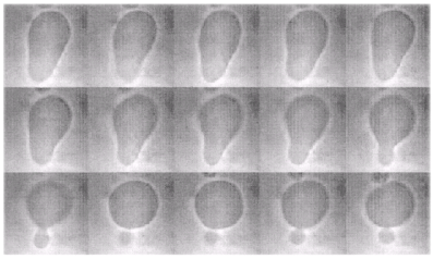
The ADE model is the generalization of the two preceding models. It was introduced in the 909090’s to explain the budding transition of some vesicles, i. e., when a vesicle adopts the shape of a parent vesicle attached through a neck to a smaller vesicle (see Fig. 1.24). The BC model predicts that this transition should be continuous, while in some experiments discontinuous transitions were observed [65].
Refer to caption
Figure 1.24: Time sequence showing the budding transition from a pear-shaped vesicle. In this case, the pear-like vesicle is instable, but it is not always the case [53].

The ADE model accounts for the fact that small relative compressions or extensions of the bilayer have an energetic cost comparable to the bending energy. Instead of a hard constraint on the area-difference between leaflets, the area-difference is regulated through an additional quadratic term in the energy, leading to

ADE=SC+κ¯2πAD2(ΔAΔA0)2,subscriptADEsubscriptSC¯𝜅2𝜋𝐴superscript𝐷2superscriptΔ𝐴Δsubscript𝐴02\mathcal{H}_{\mathrm{ADE}}=\mathcal{H}_{\mathrm{SC}}+\frac{\bar{\kappa}}{2}\frac{\pi}{AD^{2}}\left(\Delta A-\Delta A_{0}\right)^{2}\,, (1.11)

where ΔA0Δsubscript𝐴0\Delta A_{0} is the optimal area difference, also defined through

ΔA0=NoutNinϕ0,Δsubscript𝐴0subscript𝑁outsubscript𝑁insubscriptitalic-ϕ0\Delta A_{0}=\frac{N_{\mathrm{out}}-N_{\mathrm{in}}}{\phi_{0}}\,, (1.12)

where Nout/insubscript𝑁outinN_{\mathrm{out/in}} is the number of lipids on the outer/inner monolayer and ϕ0subscriptitalic-ϕ0\phi_{0} is the equilibrium density of lipid molecules. In the limiting case where κ¯0¯𝜅0\bar{\kappa}\rightarrow 0, we recover the SC model, whereas in the limit κ¯¯𝜅\bar{\kappa}\rightarrow\infty, we recover the BC model.

1.3.4 Validity of models

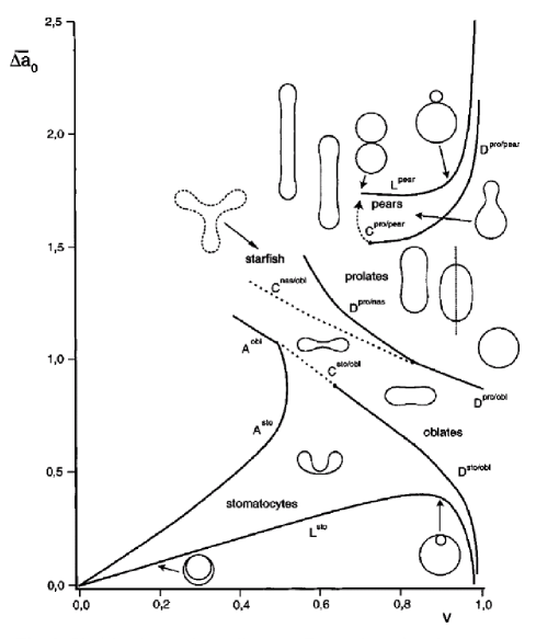
The question of which model describes the best a bilayer was not easy to answer. The main difficulty when studying vesicles comes from the fact that the three models have the same equilibrium shapes [65][67] (one can see a map of these shapes for the ADE model on Fig. 1.25 [66]). To complicate things, in certain cases, such as quasi-spherical vesicles, even the thermal fluctuations of the three models is the same [60].
Refer to caption
Figure 1.25: Phase diagram of the stationary shapes of vesicles as predicted from the ADE-model. The quantity v𝑣v is the volume-to-area ratio and Δa0¯¯Δsubscript𝑎0\overline{\Delta a_{0}} is the effective area difference (dimensionless) [66].

The three models predict however different stabilities for equilibrium shapes. For instance, the SC model predicts that pear-like vesicles should be always unstable, the BC model predicts these shapes to be always stable and the ADE model predicts stability for large values of κ¯¯𝜅\bar{\kappa}. Another difference is the nature of shape transitions induced by changes in temperature or osmotic pressure, which are in general continuous in BC and ADE and discontinuous SC.

A careful work by Döbereiner et al. [53] showed that experimental data was indeed compatible with the theoretical phase diagram for ADE-model shown in Fig. 1.25. This result was corroborated by good experimental and theoretical compatibility of the analysis of the stability and of trajectories on this phase diagrams. Nowadays, the ADE-model is accepted as the best description for closed bilayers.

There are however some situations where using SC is justifiable. First, as we have said, the models are equivalent on the study of thermal fluctuations of quasi-spherical vesicles. It is justifiable and simpler to use the SC model in this case. Besides, there is no area-difference between monolayers when these are both in contact with the same lipid reservoir and thus SC is suitable also in this case.

1.3.5 From canonical ensemble to macrocanonical

The Hamiltonian presented in the previous sections have an additional constraint in the number of lipids per membrane, or equivalently, in the total surface. In statistical mechanics, the ensemble of these constrained configurations is known as the canonical ensemble. It is a standard procedure to pass to the macrocanonical ensemble and let the area fluctuate. Physically, it means that the system we are interested in is in contact with a large reservoir of lipids, which may be a justified supposition in some cases. In this ensemble, one can control the average area by adding a term

A=σAsubscript𝐴𝜎𝐴\mathcal{H}_{A}=\sigma A (1.13)

to the Hamiltonian. The constant σ𝜎\sigma is a Lagrange-multiplier analogous to a chemical potential used to impose a certain value to the average area a posteriori, once

A=(σ),delimited-⟨⟩𝐴𝜎\langle A\rangle=\left(\frac{\partial\mathcal{F}}{\partial\sigma}\right)\,, (1.14)

where \mathcal{F} is the free-energy. The Lagrange-multiplier σ𝜎\sigma has the dimension of a tension, so sometimes it is called the surface tension, term we will avoid here. It is important to note that it is not generally measurable in experiments. It has however a measurable macroscopic counterpart r𝑟r, that we will define in the next section.

1.3.6 Fluctuation spectrum for small fluctuations

We suppose here that we study a symmetrical planar bilayer with squared projected area ApL2subscript𝐴𝑝superscript𝐿2A_{p}\equiv L^{2}, in contact with a lipid reservoir and well described by the SC model. The energy is given by

=S(2κH2+κGR1R2+σ)𝑑A.subscript𝑆2𝜅superscript𝐻2subscript𝜅𝐺subscript𝑅1subscript𝑅2𝜎differential-d𝐴\mathcal{H}=\int_{S}\left(2\kappa H^{2}+\frac{\kappa_{G}}{R_{1}R_{2}}+\sigma\right)dA\,. (1.15)

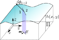
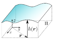
This energy will be used many times throughout this work. We will call it simply the Helfrich Hamiltonian. Consider now that the membrane is reasonably tense, so that fluctuations are small. Its position can be described by its height h(𝒓)𝒓h(\bm{r}) with respect to a plan ΠΠ\Pi parallel to the average plan, where 𝒓=(x,y)𝒓𝑥𝑦\bm{r}=(x,y) (see Fig. 1.26). This is known as the Monge gauge.
Refer to caption
Figure 1.26: Weakly fluctuating planar membrane described in the Monge gauge.

Under these assumptions, eq.(1.15) becomes

\displaystyle\mathcal{H} =\displaystyle= 0+Ap[κ2(2h)2+σ2(h)2+κGdet(hij)+𝒪(h4)]𝑑x𝑑y,subscript0subscriptsubscript𝐴𝑝delimited-[]𝜅2superscriptsuperscript22𝜎2superscript2subscript𝜅𝐺subscript𝑖𝑗𝒪superscript4differential-d𝑥differential-d𝑦\displaystyle\mathcal{H}_{0}+\int_{A_{p}}\left[\frac{\kappa}{2}\left(\nabla^{2}h\right)^{2}+\frac{\sigma}{2}\left(\nabla h\right)^{2}+\kappa_{G}\,\det(h_{ij})+\mathcal{O}(h^{4})\right]dxdy\,, (1.16)
=\displaystyle= 0+12Aph(𝒓)h(𝒓)𝑑x𝑑y+𝒪(h4)subscript012subscriptsubscript𝐴𝑝𝒓𝒓differential-d𝑥differential-d𝑦𝒪superscript4\displaystyle\mathcal{H}_{0}+\frac{1}{2}\int_{A_{p}}h(\bm{r})\,\mathcal{L}\,h(\bm{r})\,dxdy+\mathcal{O}(h^{4})

where 0=σApsubscript0𝜎subscript𝐴𝑝\mathcal{H}_{0}=\sigma A_{p} is a constant, hij2h/ijsubscript𝑖𝑗superscript2𝑖𝑗h_{ij}\equiv\partial^{2}h/\partial i\partial j, where i,j{x,y}𝑖𝑗𝑥𝑦i,j\in\{x,y\}, det(hij)=hxxhyyhxy2subscript𝑖𝑗subscript𝑥𝑥subscript𝑦𝑦superscriptsubscript𝑥𝑦2\det(h_{ij})=h_{xx}\,h_{yy}-h_{xy}^{2} and κΔ2σΔ𝜅superscriptΔ2𝜎Δ\mathcal{L}\equiv\kappa\Delta^{2}-\sigma\Delta is the operator associated to the quadratic terms of the energy.

In order to evaluate averages involving h(𝒓)𝒓h(\bm{r}), in field theory one usually adds a term proportional to an imaginary external field m(𝒓)𝑚𝒓m(\bm{r}) to the Hamiltonian, obtaining the Hamiltonian

=Aph(𝒓)m(𝒓)𝑑x𝑑y.superscriptsubscriptsubscript𝐴𝑝𝒓𝑚𝒓differential-d𝑥differential-d𝑦\mathcal{H}^{\prime}=\mathcal{H}-\int_{A_{p}}h(\bm{r})\,m(\bm{r})\,dx\,dy\,. (1.17)

The corresponding free-energy is

=kBTln(𝒵),subscript𝑘B𝑇𝒵\mathcal{F}=-k_{\mathrm{B}}T\,\ln(\mathcal{Z})\,, (1.18)

with the partition function given by the functional integral

𝒵=𝒟[h]eβ[h],𝒵𝒟delimited-[]superscript𝑒𝛽superscriptdelimited-[]\mathcal{Z}=\int\mathcal{D}[h]\,e^{-\beta\,\mathcal{H}^{\prime}[h]}\,, (1.19)

where β=1/(kBT)𝛽1subscript𝑘B𝑇\beta=1/(k_{\mathrm{B}}T). It follows

h(𝒓)𝒟[h]h(𝒓)eβ[h]eβAphm𝑑A𝒵|m=0=δδm(𝒓)|m=0delimited-⟨⟩𝒓evaluated-at𝒟delimited-[]𝒓superscript𝑒𝛽delimited-[]superscript𝑒𝛽subscriptsubscript𝐴𝑝𝑚differential-d𝐴𝒵𝑚0evaluated-at𝛿𝛿𝑚𝒓𝑚0\langle h(\bm{r})\rangle\equiv\left.\frac{\int\mathcal{D}[h]\,h(\bm{r})\,e^{-\beta\mathcal{H}[h]}\,e^{-\beta\int_{A_{p}}h\,m\,dA}}{\mathcal{Z}}\right|_{m=0}=-\left.\frac{\delta\mathcal{F}}{\delta m(\bm{r})}\right|_{m=0} (1.20)

and

h(𝒓)h(𝒓)h(𝒓)h(𝒓)=1βδ2δm(𝒓)δm(𝒓)|m=0,delimited-⟨⟩𝒓superscript𝒓delimited-⟨⟩𝒓delimited-⟨⟩superscript𝒓evaluated-at1𝛽superscript𝛿2𝛿𝑚𝒓𝛿𝑚superscript𝒓𝑚0\langle h(\bm{r})\,h(\bm{r}^{\prime})\rangle-\langle h(\bm{r})\rangle\,\langle h(\bm{r}^{\prime})\rangle=-\left.\frac{1}{\beta}\frac{\delta^{2}\mathcal{F}}{\delta m(\bm{r})\delta m(\bm{r}^{\prime})}\right|_{m=0}\,, (1.21)

where δ/δm(𝒓)𝛿𝛿𝑚𝒓\delta\mathcal{F}/\delta m(\bm{r}) represents the functional derivative of the free-energy with respect to the field m𝑚m at the point 𝒓𝒓\bm{r}.

One has now to choose an appropriate measure 𝒟[h]𝒟delimited-[]\mathcal{D}[h], which is in general a complex task [2], [68]. Up to first order on the temperature and up to second order on hh, it is justified to consider simply a discretization of the projected plan on N2superscript𝑁2N^{2} squares of area a¯2superscript¯𝑎2\bar{a}^{2} and let

𝒟naive[h]=px,pydhpx,pyλ,subscript𝒟naivedelimited-[]subscriptproductsubscript𝑝𝑥subscript𝑝𝑦𝑑superscriptsubscript𝑝𝑥subscript𝑝𝑦𝜆\mathcal{D}_{\mathrm{naive}}[h]=\prod_{p_{x},p_{y}}\frac{dh^{p_{x},p_{y}}}{\lambda}\,, (1.22)

where hpx,pysuperscriptsubscript𝑝𝑥subscript𝑝𝑦h^{p_{x},p_{y}} is the height at the point 𝒓px,py=pxa¯𝒆x+pya¯𝒆ysubscript𝒓subscript𝑝𝑥subscript𝑝𝑦subscript𝑝𝑥¯𝑎subscript𝒆𝑥subscript𝑝𝑦¯𝑎subscript𝒆𝑦\bm{r}_{p_{x},p_{y}}=p_{x}\,\bar{a}\,\bm{e}_{x}+p_{y}\,\bar{a}\,\bm{e}_{y}, λ𝜆\lambda is a length introduced to render the measure dimensionless and both pxsubscript𝑝𝑥p_{x} and pysubscript𝑝𝑦p_{y} {1,,N}absent1𝑁\in\{1,\cdots,N\}  [2]. This measure, which we will call naive as in ref.[2], yields no supplemental term to the Hamiltonian.

Evaluating the Gaussian integrals on eq.(1.19), one obtains

𝒵=Ceβ2Apm(𝒓)1(𝒓,𝒓)m(𝒓)𝑑x𝑑y,𝒵𝐶superscript𝑒𝛽2subscriptsubscript𝐴𝑝𝑚𝒓superscript1𝒓superscript𝒓𝑚superscript𝒓differential-d𝑥differential-d𝑦\mathcal{Z}=C\,e^{\frac{\beta}{2}\int_{A_{p}}m(\bm{r})\,\mathcal{H}^{-1}(\bm{r},\bm{r}^{\prime})\,m(\bm{r}^{\prime})\,dxdy}\,, (1.23)

with C𝐶C a constant and 1(𝒓,𝒓)Γ(𝒓𝒓)superscript1𝒓superscript𝒓Γsuperscript𝒓𝒓\mathcal{H}^{-1}(\bm{r},\bm{r}^{\prime})\equiv\Gamma(\bm{r}^{\prime}-\bm{r}) solution of

Γ(𝒓)=δ(𝒓),Γ𝒓𝛿𝒓\mathcal{L}\,\Gamma(\bm{r})=\delta(\bm{r})\,, (1.24)

where δ(𝒓)𝛿𝒓\delta(\bm{r}) is Dirac’s delta function. Using the Fourier transform

Γ(𝒓)=1L𝒒Γn,mei𝒒𝒓,Γ𝒓1𝐿subscript𝒒subscriptΓ𝑛𝑚superscript𝑒𝑖𝒒𝒓\Gamma(\bm{r})=\frac{1}{L}\sum_{\bm{q}}\Gamma_{n,m}\,e^{i\,\bm{q}\cdot\bm{r}}\,, (1.25)

with 𝒒=2π/L(n,m)𝒒2𝜋𝐿𝑛𝑚\bm{q}=2\pi/L\,(n,m), n,m𝑛𝑚n,m\in\mathbb{N} and

𝒒|n|Nmax|m|Nmax,subscript𝒒subscript𝑛subscript𝑁maxsubscript𝑚subscript𝑁max\sum_{\bm{q}}\equiv\sum_{|n|\,\leq\,N_{\mathrm{max}}}\,\sum_{|m|\,\leq\,N_{\mathrm{max}}}\,, (1.26)

where Nmax=L/(2a¯)subscript𝑁max𝐿2¯𝑎N_{\mathrm{max}}=L/(2\bar{a}) corresponds to smallest possible wave-length, eq.(1.24) yields

Γn,m=1σq2+κq4.subscriptΓ𝑛𝑚1𝜎superscript𝑞2𝜅superscript𝑞4\Gamma_{n,m}=\frac{1}{\sigma q^{2}+\kappa q^{4}}\,. (1.27)

From eq.(1.20) and eq.(1.21), one obtains respectively h(𝒓)=0delimited-⟨⟩𝒓0\langle h(\bm{r})\rangle=0 and the correlation function

h(𝒓)h(𝒓)=kBTAp𝒒ei𝒒(𝒓𝒓)σq2+κq4.delimited-⟨⟩𝒓superscript𝒓subscript𝑘B𝑇subscript𝐴𝑝subscript𝒒superscript𝑒𝑖𝒒𝒓superscript𝒓bold-′𝜎superscript𝑞2𝜅superscript𝑞4\langle h(\bm{r})h(\bm{r}^{\prime})\rangle=\frac{k_{\mathrm{B}}T}{A_{p}}\sum_{\bm{q}}\frac{e^{i\,\bm{q}\cdot(\bm{r}-\bm{r^{\prime}})}}{\sigma q^{2}+\kappa q^{4}}\,. (1.28)

Note that the Gaussian curvature contribution vanishes. Applying the Fourier transform as defined above to h(𝒓)𝒓h(\bm{r}) and h(𝒓)superscript𝒓h(\bm{r}^{\prime}) in eq.(1.28), one obtains

|hn,m|2=kBTσq2+κq4,delimited-⟨⟩superscriptsubscript𝑛𝑚2subscript𝑘B𝑇𝜎superscript𝑞2𝜅superscript𝑞4\langle|h_{n,m}|^{2}\rangle=\frac{k_{\mathrm{B}}T}{\sigma q^{2}+\kappa q^{4}}\,, (1.29)

where the wave vectors range from qmin=2π/Lsubscript𝑞min2𝜋𝐿q_{\mathrm{min}}=2\pi/L to an upper cut-off Λ=2πNmax/L1/a¯Λ2𝜋subscript𝑁max𝐿1¯𝑎\Lambda=2\pi N_{\mathrm{max}}/L\approx 1/\bar{a}. Throughout this work, we shall consider that numerically a¯a¯𝑎𝑎\bar{a}\equiv a, where a𝑎a is of the order of the membrane thickness. Remark that since h(𝒓)𝒓h(\bm{r}) is real, we have hn,m=hn,msubscript𝑛𝑚superscriptsubscript𝑛𝑚h_{-n,-m}=h_{n,m}^{*}, where the symbol stands for the complex conjugate, yielding |hn,m|=|hn,m|subscript𝑛𝑚subscript𝑛𝑚|h_{-n,-m}|=|h_{n,m}|.

Similar calculations can be carried out for non-planar membranes, yielding a correlation function similar eq.(1.28). Consequently, by measuring the fluctuations of a membrane, one could deduce its bending rigidity and the tension σ𝜎\sigma. The problem is that experimentally we have access only to a coarse-grained vision of the membrane. One has thus to consider that the values deduced from the fluctuation spectrum are in fact renormalized values, which we will call κeffsubscript𝜅eff\kappa_{\mathrm{eff}} for the bending rigidity and r𝑟r for the effective tension. Renormalization calculations [69] indicate that

κeff=κ3kBT4πln(La),subscript𝜅eff𝜅3subscript𝑘B𝑇4𝜋𝐿𝑎\kappa_{\mathrm{eff}}=\kappa-\frac{3k_{\mathrm{B}}T}{4\pi}\ln\left(\frac{L}{a}\right)\,, (1.30)

where L𝐿L is the size of the membrane and a𝑎a is a microscopical cut-off. Experimentally, the dependence of κeffsubscript𝜅eff\kappa_{\mathrm{eff}} as a function of L𝐿L is very difficult to measure, since the dependence is logarithmic. Numerical simulations however confirmed the logarithmic dependence on L𝐿L [70]. For a rough numerical estimate, if we consider a vesicle with radius R10μm𝑅10𝜇mR\approx 10\,\mathrm{\mu m} and we consider the cut-off of the order of the membrane thickness a5nm𝑎5nma\approx 5\,\mathrm{nm}, we obtain κeffκ2kBTsubscript𝜅eff𝜅2subscript𝑘B𝑇\kappa_{\mathrm{eff}}\approx\kappa-2k_{\mathrm{B}}T. The correction is thus one order of magnitude smaller than typical values of κ𝜅\kappa. Henceforth, we will assume κeffκsubscript𝜅eff𝜅\kappa_{\mathrm{eff}}\equiv\kappa. The distinction between r𝑟r and σ𝜎\sigma will however be kept and discussed throughout this paper.

1.4 Experiments

Here we present some current experimental apparatus and techniques used to measure the relevant mechanical parameters κ𝜅\kappa, K𝐾K, τ𝜏\tau, r𝑟r and α𝛼\alpha. We will not mention neither measures of κ¯¯𝜅\bar{\kappa}, since we will focus on symmetrical membranes, neither measures of κGsubscript𝜅𝐺\kappa_{G}, since we will work with closed membranes of fixed topology (in the case of non-closed membranes, we will show it is not relevant in section 1.5). In section 1.4.5, we sum up these experiments.

1.4.1 Micropipette experiments

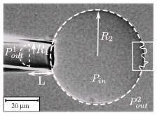
In these experiments, a micropipette of some micrometers of diameter is held in contact with a vesicle. One increases the membrane tension by decreasing the pressure Pout1superscriptsubscript𝑃out1P_{\mathrm{out}}^{1} on the pipette. A portion of the membrane of length L𝐿L is then sucked inside the pipette and the optical resolvable surface Apsubscript𝐴𝑝A_{p} increases (see Fig. 1.27).

Refer to caption
Refer to caption
Refer to caption
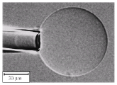
Figure 1.27: The upper figures show typical micrographs of vesicles under suction for increasing values of ΔPΔ𝑃\Delta P (extracted from [71]). The lower drawing indicates the measurable quantities. The inset on the right represents a zoom of the microscopic fluctuations that are averaged out in these micrographs.

Usually, successive measures with increasing pressure are taken. The first configuration, when the vesicle is just grabbed by the pipette and L𝐿L is small, is the reference configuration. The projected area of this configuration is Apisuperscriptsubscript𝐴𝑝𝑖A_{p}^{i}, R1subscript𝑅1R_{1} is the radius of the micropipette and R2subscript𝑅2R_{2} is the radius of the vesicle in the reference configuration. Under the condition of constant volume and R2R1much-less-thansubscript𝑅2subscript𝑅1R_{2}\ll R_{1}, the percent difference on the projected area of a posterior measure whose projected area is Apfsuperscriptsubscript𝐴𝑝𝑓A_{p}^{f} is given by

ApfApiApi=12[(R1R2)2(R1R2)3]ΔLR1γ,superscriptsubscript𝐴𝑝𝑓superscriptsubscript𝐴𝑝𝑖superscriptsubscript𝐴𝑝𝑖12delimited-[]superscriptsubscript𝑅1subscript𝑅22superscriptsubscript𝑅1subscript𝑅23Δ𝐿subscript𝑅1𝛾\frac{A_{p}^{f}-A_{p}^{i}}{A_{p}^{i}}=\frac{1}{2}\left[\left(\frac{R_{1}}{R_{2}}\right)^{2}-\left(\frac{R_{1}}{R_{2}}\right)^{3}\right]\frac{\Delta L}{R_{1}}\gamma\,, (1.31)

where ΔLΔ𝐿\Delta L is the length variation of the cylinder sucked inside the pipette relative to the reference measure and γ𝛾\gamma is a corrective factor which arises when L𝐿L is non zero in the reference configuration [72].

Meanwhile, the average applied tension can be related to the difference of pressure ΔP=Pout2Pout1Δ𝑃superscriptsubscript𝑃out2superscriptsubscript𝑃out1\Delta P=P_{\mathrm{out}}^{2}-P_{\mathrm{out}}^{1} through the Young–Laplace equation [73]. For a very thin interface under tension τ𝜏\tau and whose principal curvature radii are Rsuperscript𝑅R^{\prime} and R′′superscript𝑅′′R^{\prime\prime}, it states

ΔP=τ(1R+1R′′).Δ𝑃𝜏1superscript𝑅1superscript𝑅′′\Delta P=\tau\left(\frac{1}{R^{\prime}}+\frac{1}{R^{\prime\prime}}\right)\,. (1.32)

For the system shown in Fig. 1.27, one obtains thus the relation

PinPout2=2τR2subscript𝑃insuperscriptsubscript𝑃out22𝜏subscript𝑅2P_{\mathrm{in}}-P_{\mathrm{out}}^{2}=\frac{2\tau}{R_{2}} (1.33)

for the largest part of the vesicle and

PinPout1=2τR1subscript𝑃insuperscriptsubscript𝑃out12𝜏subscript𝑅1P_{\mathrm{in}}-P_{\mathrm{out}}^{1}=\frac{2\tau}{R_{1}} (1.34)

for the spherical cap inside the micropipette. Finally, by subtracting eq.(1.33) from eq.(1.34), one obtains

ΔP=Pout2Pout1=2τ(1R11R2).Δ𝑃superscriptsubscript𝑃out2superscriptsubscript𝑃out12𝜏1subscript𝑅11subscript𝑅2\Delta P=P_{\mathrm{out}}^{2}-P_{\mathrm{out}}^{1}=2\tau\left(\frac{1}{R_{1}}-\frac{1}{R_{2}}\right)\,. (1.35)

For very small pipettes or for vesicles under very weak tension, this relation must be corrected [74]. Through this technique, one can apply a wide range of tensions on membranes, from very small ones (109N/msimilar-toabsentsuperscript109Nm\sim 10^{-9}\,\mathrm{N/m}) up to rupture tensions (102N/msimilar-toabsentsuperscript102Nm\sim 10^{-2}\,\mathrm{N/m}[55][75].

Theoretically, calculations in the macrocanonical ensemble predict two regimes: one at low tension, where it comes from the flattening of fluctuations and thus [52][73] (see section 2.4 for a detailed derivation)

ApfApiApi=kBT8πκln(σfσi),superscriptsubscript𝐴𝑝𝑓superscriptsubscript𝐴𝑝𝑖superscriptsubscript𝐴𝑝𝑖subscript𝑘B𝑇8𝜋𝜅subscript𝜎𝑓subscript𝜎𝑖\frac{A_{p}^{f}-A_{p}^{i}}{A_{p}^{i}}=\frac{k_{\mathrm{B}}T}{8\pi\kappa}\ln\left(\frac{\sigma_{f}}{\sigma_{i}}\right)\,, (1.36)

where σi/fsubscript𝜎𝑖𝑓\sigma_{i/f} is respectively the Lagrange-multiplier for the initial/final configuration; and one at high tension, where it arises mainly through stretching and thus

ApfApiApi=σfK.superscriptsubscript𝐴𝑝𝑓superscriptsubscript𝐴𝑝𝑖superscriptsubscript𝐴𝑝𝑖subscript𝜎𝑓𝐾\frac{A_{p}^{f}-A_{p}^{i}}{A_{p}^{i}}=\frac{\sigma_{f}}{K}\,. (1.37)

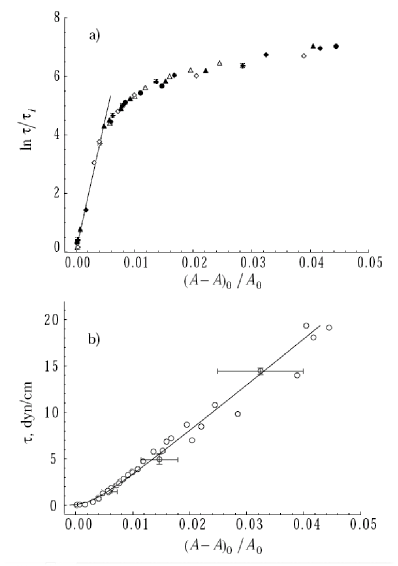
Even though these previsions involve the non-measurable Lagrange-multiplier σ𝜎\sigma, in experiments it is currently assumed that στ𝜎𝜏\sigma\approx\tau  [72][73][76]. As a consequence, by plotting τ𝜏\tau as a function of the variation of the projected, one can measure κ𝜅\kappa and K𝐾K (see an example in Fig. 1.28).

Refer to caption
Figure 1.28: Graphics showing a typical data analysis of micropipette experiments [76]. Fig.(a) and Fig.(b) show the same data with different scales for τ𝜏\tau. In Fig.(a), the tensions were displayed in log-scale in order to highlight the logarithmic behavior in the region of low tension. Through the fit shown in Fig.(a) and using eq.(1.36), one measures the bending rigidity (κ=42±5kBT𝜅plus-or-minus425subscript𝑘B𝑇\kappa=42\pm 5\,k_{\mathrm{B}}T in these measures). Fig.(b) shows the same data in the linear scale. The area compressibility K𝐾K is obtained through a fit in the region of high tensions using eq.(1.37) (K=450±85mN/m𝐾plus-or-minus45085mNmK=450\pm 85\,\mathrm{mN/m} here). Remark that it was assumed that στ𝜎𝜏\sigma\approx\tau.
1.4.2 Contour analysis experiments

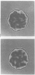
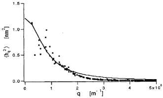
The aim of these experiments is to determine r𝑟r and κ𝜅\kappa by studying the mean squared amplitude of fluctuating modes, as seen on section 1.3.6. Some experiments were made in planar geometry, using BLM. As explained before, these membranes tend to be too tense. Indeed, a 1999 experiment by Hirn et al. found r=(0.42±0.03)mN/m𝑟plus-or-minus0.420.03mNmr=(0.42\pm 0.03)\,\mathrm{mN/m} [77]. The fluctuations are then dominated by the tension and one cannot observe the effects of the bending rigidity. For this reason vesicles are usually preferred in spectrum fluctuation measures. A typical spectrum with the fitting can be seen in Fig. 1.29.
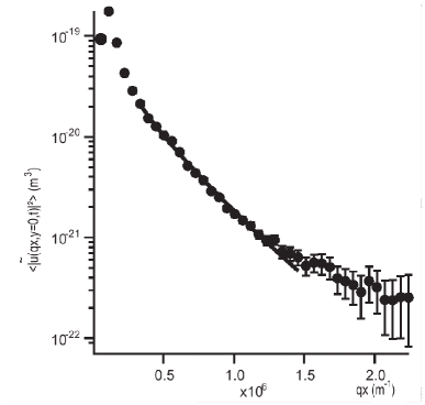
Refer to caption
Figure 1.29: Intensity of a fluctuating mode as a function of the wave vector for a quasi-spherical vesicle. The solid line represents the fit of the data with the equivalent of eq.(1.29) for spherical geometry, yielding κ=9.44×10²⁰J𝜅9.44superscript1020J\kappa=9.44\times 10^{-20}\,\mathrm{J} and r=1.74×10⁷N/m𝑟1.74superscript107Nmr=1.74\times 10^{-7}\,\mathrm{N/m} [78].
1.4.3 Adhesion of vesicles

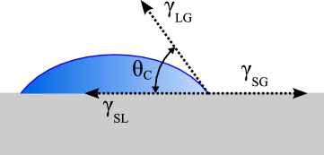
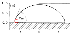
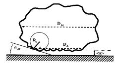
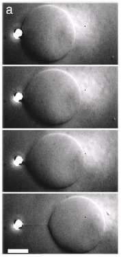
The adhesion of membranes is very important for tissue formation. At the cellular level, the adhesion between the membrane and the cytoskeleton helps to regulate the formation of vesicles and lamellipodia [79]. It also plays an important role in the exocytosis and endocytosis [80]. In the context of the physics of liquids, the adhesion of liquid drops to solid substrates is traditionally used to study tensions. Inspired by these experiments, one finds in the literature a wide variety of papers on the adhesion of vesicles among themselves [81][82] and on the adhesion of vesicles with a solid substrate [83][84][85][86].

Here, we will focus on experiments dealing with the interaction of vesicles of radius Rvessubscript𝑅vesR_{\mathrm{ves}} with a flat solid substrate. The vesicle, usually filled with an aqueous solution fluid denser than the suspension medium, is attracted towards the bottom surface. At equilibrium, it adopts a deformed shape as shown in Fig. 1.22, with a flat region near the substrate. This region, with a radius Rasubscript𝑅𝑎R_{a}, is considered adhered to the substrate. Frequently, the bottom surface is composed of glass, since the technique of RICM (reflection interference contrast microscopy) is very popular to obtain images of the adhesion region. The adhesion is ruled by the interplay of attractive and repulsive interactions, such as:

  • the short-range van der Waals attractive potential between the membrane and the substrate. It can be corrected to take into account the screening due to the presence of ions in the suspension medium;

  • the attractive gravitational potential;

  • the repulsive effective interaction coming from the reduction of the entropy of the membrane. Indeed, the substrate imposes a spatial restriction that limits the membrane fluctuations;

  • the short-range steric repulsion coming from the lipids;

  • in some cases, the substrate can be coated by polymers [87]. One must thus consider a supplemental steric repulsion coming from the polymer coating of the substrate;

  • it is also possible to cover the substrate with a piece of membrane containing proteins that attach to specific proteins embedded in the vesicle’s membrane [85][88]. In this case, there are supplemental attractive interactions.

Two examples of resulting potentials can be seen in Fig. 1.30.
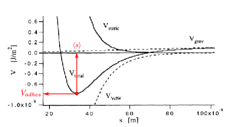
Refer to caption
(a) An adhesion potential including the gravity contribution Vgravsubscript𝑉gravV_{\mathrm{grav}}, a Van der Waals contribution VVdWsubscript𝑉VdWV_{\mathrm{VdW}} and an entropic repulsive term Vstericsubscript𝑉stericV_{\mathrm{steric}} [84]. In this case, we find only one shallow minimum.
Refer to caption
(b) Predicted adhesion potential for an experiment involving three different polymer coatings of the substrate [87]. The red circles indicate the deep minima and the star indicates the shallow minimum.
Figure 1.30: Examples of adhesion potentials.

Depending on the resulting potential, one can find two types of adhesion:

  1. 1.

    Weak adhesion: in this case, the adhering patch fluctuates strongly at a distance s(x)𝑠𝑥s(x) well above the surface, as shown in Fig. 1.33(b). It corresponds to a shallow minimum of the adhesion potential (see Fig. 1.30). When it is a local minimum, it is also said that the vesicle is in a pre-nucleation state.

    In this case, one can measure the fluctuation spectrum of the adhering region. Considering the rest of the vesicle as a lipid reservoir and approximating the energy of adhesion as quadratic near sdelimited-⟨⟩𝑠\langle s\rangle, which is justified given Fig. 1.30, the Hamiltonian up to order two is given by [84]

    =Sadhe[κ2(2h)2+σ2(h)2+V′′2h2]d2𝒙,subscriptsubscript𝑆adhedelimited-[]𝜅2superscriptsuperscript22𝜎2superscript2superscript𝑉′′2superscript2superscript𝑑2𝒙\mathcal{H}=\int_{S_{\mathrm{adhe}}}\left[\frac{\kappa}{2}\left(\nabla^{2}h\right)^{2}+\frac{\sigma}{2}\left(\nabla h\right)^{2}+\frac{V^{\prime\prime}}{2}h^{2}\right]d^{2}\bm{x}\,, (1.38)

    where h(𝒙)=s(𝒙)s𝒙𝑠𝒙delimited-⟨⟩𝑠h(\bm{x})=s(\bm{x})-\langle s\rangle, V′′superscript𝑉′′V^{\prime\prime} is the coefficient of the harmonic approximation of the adhesion energy and Sadhesubscript𝑆adheS_{\mathrm{adhe}} is the projected surface of the adhering portion of the vesicle. Following the same reasoning presented in section 1.3.6, the mean square amplitude of each mode is given by

    |h(𝒒)|2=kBTV′′+rq2+κq4.delimited-⟨⟩superscript𝒒2subscript𝑘B𝑇superscript𝑉′′𝑟superscript𝑞2𝜅superscript𝑞4\langle|h(\bm{q})|^{2}\rangle=\frac{k_{\mathrm{B}}T}{V^{\prime\prime}+rq^{2}+\kappa q^{4}}\,. (1.39)

    Note that we have substituted σ𝜎\sigma by its macroscopical counterpart r𝑟r, which is experimentally measurable (see further details in the end of section 1.3.6). By a measuring the fluctuation spectrum, it is possible thus to determine r𝑟r, κ𝜅\kappa and V′′superscript𝑉′′V^{\prime\prime}.

  2. 2.

    Strong adhesion: the vesicle is very near the substrate (less than 10nm10nm10\,\mathrm{nm} of distance). The membrane fluctuations are barely detectable. The adhesion energy is higher, corresponding to a deep minimum of the adhesion potential.

In Fig. 1.31, we show some typical RICM images from an adhering vesicle that has weakly and strongly adhering patches. From these images, the height profile of the adhesion region s(x)𝑠𝑥s(x) can be reconstructed. One can subsequently study the mechanics of the membrane.
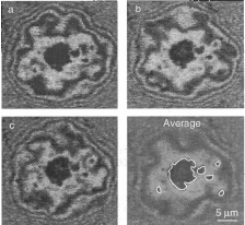
Refer to caption
Figure 1.31: RICM micrograph of a vesicle adhering to a solid substrate. The adhering region is surrounded by the fringes. The gray shading is inversely proportional to the vesicle-substrate distance: the dark gray patch is very near to the substrate, while the light gray patch is well above the solid. Pictures (a), (b) and (c) were taken at 0.1ssimilar-toabsent0.1s\sim 0.1\mathrm{s} of interval. Note the strong fluctuations of the light gray region. The last picture shows the average over 646464 snapshots. From these images, we can conclude that the gray region adheres only weakly to the substrate, while the dark patch is strongly adhered [88].
Adhesion mechanics

Let’s first recall some results concerning liquid drops. As discussed in section 1.2.2, the contact angle θcsubscript𝜃𝑐\theta_{c} that liquid drops do with solids substrate is very sharp. It is defined by the solid-liquid tension γSLsubscript𝛾𝑆𝐿\gamma_{SL}, the solid-gas tension γSGsubscript𝛾𝑆𝐺\gamma_{SG} and the liquid-gas solid γγLG𝛾subscript𝛾𝐿𝐺\gamma\equiv\gamma_{LG}. The mechanical equilibrium, illustrated in Fig. 1.32, gives the Young relation

γSG=γSL+γcosθc.subscript𝛾𝑆𝐺subscript𝛾𝑆𝐿𝛾subscript𝜃𝑐\gamma_{SG}=\gamma_{SL}+\gamma\cos\theta_{c}\,. (1.40)

The energy variation per unit of contact area between the liquid and the solid, also known as the adhesion energy per unit area, is given by the Young-Dupree relation:

WA=γ(1cosθc).subscript𝑊𝐴𝛾1subscript𝜃𝑐W_{A}=\gamma(1-\cos\theta_{c})\,. (1.41)
Refer to caption
Figure 1.32: Illustration of the Young’s equation: γSLsubscript𝛾𝑆𝐿\gamma_{SL} is the solid-liquid tension, γSGsubscript𝛾𝑆𝐺\gamma_{SG} is the solid-gas tension and γγLG𝛾subscript𝛾𝐿𝐺\gamma\equiv\gamma_{LG} is the liquid-gas tension. The contact angle θcsubscript𝜃𝑐\theta_{c} is defined by the mechanical equilibrium.

Adhering vesicles were first theoretically studied in details by Seifert et Lipowsky in 1990 [80]. They considered a free-energy containing a contribution from curvature, a term WA(πRa2)subscript𝑊𝐴𝜋superscriptsubscript𝑅𝑎2-W_{A}\,(\pi R_{a}^{2}) corresponding to the adhesion energy plus the area and volume constraints. By minimizing the free-energy, they derived the equilibrium shapes, that shared two features:

  • a contact angle θc=πsubscript𝜃𝑐𝜋\theta_{c}=\pi due to the bending rigidity;

  • a curvature at the contact given by

    Rc=(2WAκ)1/2.subscript𝑅𝑐superscript2subscript𝑊𝐴𝜅12R_{c}=\left(\frac{2\,W_{A}}{\kappa}\right)^{1/2}\,. (1.42)

They argued that, in general, one could not expect to use the Young-Dupree relation to link WAsubscript𝑊𝐴W_{A} and the lateral tension τ𝜏\tau of the membrane due to the effects of the bending rigidity. In the limit, however, of small bending rigidity, the vesicle becomes a spherical cap for an internal pressure bigger than the outer, with a rounded contact region of length Rc<Rvessubscript𝑅𝑐subscript𝑅vesR_{c}<R_{\mathrm{ves}}. One can thus define an effective contact angle θeffsubscript𝜃eff\theta_{\mathrm{eff}} (see Fig. 1.33(a)) that obeys an analogous of the Young-Dupree equation

WA=τ[1cos(θeff)].subscript𝑊𝐴𝜏delimited-[]1subscript𝜃effW_{A}=\tau\left[1-\cos(\theta_{\mathrm{eff}})\right]\,. (1.43)
Refer to caption
(a) Definition of the effective contact angle. The red circle at left indicates the curvature radius Rcsubscript𝑅𝑐R_{c} at the contact point. Note that Rc<Rvessubscript𝑅𝑐subscript𝑅vesR_{c}<R_{\mathrm{ves}} [80].
Refer to caption
(b) Drawing of a vesicle weakly adhering to a substrate with the relevant measurable parameters [84].
Figure 1.33: Effective contact angle.

In principle, for a vesicle under these conditions, one could measure Rcsubscript𝑅𝑐R_{c} and θeffsubscript𝜃eff\theta_{\mathrm{eff}} and thus deduce WAsubscript𝑊𝐴W_{A} and τ𝜏\tau. In practice, however, as we will see later, measuring these quantities can be very tricky and imprecise.

An alternative was thus proposed by Bruinsma [89]. He studied the equilibrium of the forces due to the bending rigidity and tension near the rim of the contact region and obtained

h(x)={θeffxθeffλ[1e(xλ)]forx>0,0forx<0,𝑥casessubscript𝜃eff𝑥subscript𝜃eff𝜆delimited-[]1superscript𝑒𝑥𝜆for𝑥0missing-subexpressionmissing-subexpressionmissing-subexpression0for𝑥0h(x)=\left\{\begin{array}[]{ccc}\theta_{\mathrm{eff}}\,x-\theta_{\mathrm{eff}}\,\lambda\left[1-e^{-\left(\frac{x}{\lambda}\right)}\right]&$for$&\,x>0\,,\\ \\ 0&$for$&\,x<0\,,\end{array}\right. (1.44)

where h(x)𝑥h(x) is the height of the membrane, x=0𝑥0x=0 at the contact point and

λ=κτ.𝜆𝜅𝜏\lambda=\sqrt{\frac{\kappa}{\tau}}\,. (1.45)

The characteristic length λ𝜆\lambda separates two regions: for x<λ𝑥𝜆x<\lambda, the bending rigidity dominates and the membrane is thus curve; for x>λ𝑥𝜆x>\lambda, the tension dominates and the membrane approaches a straight line (see Fig. 1.34).
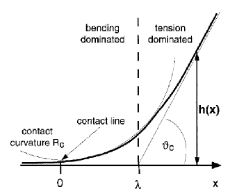
Refer to caption
Figure 1.34: Shape of the membrane near the contact region. For x<0𝑥0x<0, the membrane adheres to the substrate. The contact angle θeffsubscript𝜃eff\theta_{\mathrm{eff}}, here shown as θcsubscript𝜃𝑐\theta_{c}, is determined by the linear fit. The characteristic length λ𝜆\lambda is obtained from the intersection of the linear fit with the x𝑥x-axis [90].

Experimentally, from the height profile of the membrane, one can obtain θeffsubscript𝜃eff\theta_{\mathrm{eff}} and λ𝜆\lambda. Using eq.(1.45) one is able thus to deduce τ𝜏\tau and subsequently WAsubscript𝑊𝐴W_{A} through the Young-Dupree’s relation [88]. This method, however, presents a serious limitation: if the tension is very large, the length λ𝜆\lambda is undetectable [86]. In the next chapter, we will discuss some experiments using these techniques.

1.4.4 Nanotube extraction

Membrane nanotubes, also called tethers, are cylindrical structures whose radius range from a few up to hundreds of nanometers, while their length can reach tens of micrometers. In living cells, they are formed by localized forces generated by molecular motors or by polymerizing cytoskeleton filaments, such as microtubules. These tethers are suspected to play a major hole in the intracellular transport of vesicles [91] and in the communication between cells, since they form also between different cells and proteins were shown to pass through these tunneling nanotubes (TNT) [92] (see Fig. 1.35). Recently, it has been found some evidence that TNT may even be crucial in the HIV virus spreading [93].
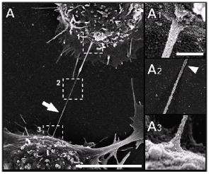
Refer to caption
Figure 1.35: Scanning electron microscopic image of a tunneling tube between two cultured PC12 cells. The boxed areas are sections of 80nm80nm80\,\mathrm{nm} enlarged in A1, A2 and A3, respectively [94].

In vitro tube extraction was used to evaluate the adhesion energy between the cell cytoskeleton and the cell membrane. In these experiments, it was also shown that these tethers do not contain cytoskeleton [79][95]. Here we will restrain ourselves to experiments of tube extraction from model membranes (see Fig. 1.36(a)). Figs. 1.36(b)-1.36(c) sum up the main techniques used in laboratory to extract tubes.

In typical experiments with GUVs, one cannot optically resolve the tube, even though its length is readily measurable (see Fig. 1.36(a)). The force needed to extract the tube f𝑓f can be directly measured by the force applied over the glass bead (for an optical tweezer) or over the magnetic bead. Moreover, if the vesicle is held by a micropipette, as in the experimental apparatus shown in Fig. 1.36(b), subfigure b, the tension τ𝜏\tau is measured through the applied pressure from eq.(1.35[96]. Another technique consists in extracting nanotubes with controlled length from BLMs. With this configuration, it is possible to apply a difference of electrical potential between the interior and exterior of the tube. One can thus deduce the radius of the tube and the tension τ𝜏\tau of the membrane [97].

From the theoretical point of view, as these tubes are so thin, it is reasonable to consider the adjacent GUV or BLM as a lipid reservoir. For a symmetrical membrane, the tube free energy is thus given by eq.(1.15) plus a contribution coming from the force f𝑓f that holds the tube. For a cylindrical tube of radius R𝑅R and length L𝐿L, one has

=(κ2R2+σ)2πRLfL.𝜅2superscript𝑅2𝜎2𝜋𝑅𝐿𝑓𝐿\mathcal{H}=\left(\frac{\kappa}{2R^{2}}+\sigma\right)2\pi RL-fL\,. (1.46)
Refer to caption
(a) Typical sequence of nanotube extraction from a GUV. The image was obtained through differential interference contrast microscopy to enhance contrast, since the tube is not optically resolvable [98].
Refer to caption
(b) Some methods used to extract tubes from GUV: (a) vesicles under hydrodynamic flow [99], (b) vesicles held by micropipette and attached to a mobile glass or magnetic bead [96],  [100] and (c) nanotube extraction with molecular motors [101].
Refer to caption
(c) Experimental setting used to extract nanotubes from BLM [97].
Figure 1.36: Nanotube extraction techniques.

The equilibrium radius R0subscript𝑅0R_{0} and force f0subscript𝑓0f_{0} are given by the minimization of eq.(1.46) with respect to R𝑅R and L𝐿L respectively, yielding

R0=κ2σsubscript𝑅0𝜅2𝜎R_{0}=\sqrt{\frac{\kappa}{2\sigma}} (1.47)

and

f0=2π2σκ=2×2πR0σ.subscript𝑓02𝜋2𝜎𝜅22𝜋subscript𝑅0𝜎f_{0}=2\pi\sqrt{2\sigma\kappa}=2\times 2\pi R_{0}\,\sigma\,. (1.48)

Eq.(1.47) shows clearly that the radius is determined by a competition between the tension, which tends to create a very thin tube, and the bending rigidity, which opposes to high curvatures [102]. Interestingly, the result given in eq.(1.48) highlights the difference between a membrane and a liquid interface: if we had a tube constituted by a film of liquid, we should expect f=2πR0γ𝑓2𝜋subscript𝑅0𝛾f=2\pi R_{0}\gamma. The factor 222 in f0subscript𝑓0f_{0} comes from the curvature energy present only in membranes. One must keep in mind that these results hold only if thermal fluctuations are neglected and the tube is a perfect cylinder. We will discuss this point in chapter 5.
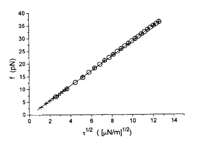
Refer to caption
Figure 1.37: Data from the extraction of two successive tubes from the same vesicle of diameter 18.8μm18.8𝜇m18.8\,\mathrm{\mu m}. The vertical axis shows the force needed to extract the tube while the horizontal axis shows the square root of the tension τ𝜏\tau measured through the difference of pressure in the micropipette. The data show a good linear fit, indicating that in this experiment, it was apparently justified to neglect thermal undulations and suppose στ𝜎𝜏\sigma\approx\tau. The bending rigidity obtained through the fit is approximately 25kBT25subscript𝑘B𝑇25\,k_{\mathrm{B}}T [96]. By using eq.(1.47), we can estimate that the tube radius are rather large, ranging from a thousand to two hundred nanometers in this particular experiment.

From eq.(1.48), we see that one could obtain κ𝜅\kappa by measuring f0subscript𝑓0f_{0} and σ𝜎\sigma. In GUV experiments, it is usually assumed that the measured force to extract the tube f𝑓f is well approximated by f0subscript𝑓0f_{0}, which means neglecting thermal undulations. Besides, the tension τ𝜏\tau measured through the micropipette aspiration is assumed equivalent to σ𝜎\sigma. One obtains thus the curve shown in Fig. 1.37 and deduces κ𝜅\kappa by a linear fit. The other way to obtain κ𝜅\kappa, using eq.(1.47), is explored in the BLM experiments by once more assuming that τσ𝜏𝜎\tau\approx\sigma. A recent experiment by Bashkirov [97] found very thin tubes of about 10nm10nm10\,\mathrm{nm} thick, indicating a very tense membrane, and deduced values to κ𝜅\kappa compatible with previous results.

1.4.5 Sum-up

In table 1.1, we see a sum-up of the techniques presented in this section and used to mechanically probe membranes. In the last column, we can see the usual assumption made in order to deduce results from the third column. It generally involves the three tensions τ𝜏\tau, σ𝜎\sigma and r𝑟r. In this work, we will try to examine in detail these assumptions. In special, we will quantify the difference between τ𝜏\tau and σ𝜎\sigma for the three mainly studied geometries and discuss under which conditions these suppositions are justifiable. In chapter 5, we will also examine the role of thermal fluctuations on the force needed to extract a tube.

Technique Direct measure Used to deduce Usual assumption
micropipette ΔPΔ𝑃\Delta P, Apsubscript𝐴𝑝A_{p} τ𝜏\tau, ΔαΔ𝛼\Delta\alpha, κ𝜅\kappa, K στ𝜎𝜏\sigma\approx\tau
contour analysis |h(𝒒)|2delimited-⟨⟩superscript𝒒2\langle|h(\bm{q})|^{2}\rangle r, κ𝜅\kappa
adhesion θeffsubscript𝜃eff\theta_{\mathrm{eff}}, |h(𝒒)|2delimited-⟨⟩superscript𝒒2\langle|h(\bm{q})|^{2}\rangle, sdelimited-⟨⟩𝑠\langle s\rangle r, κ𝜅\kappa, Wadhessubscript𝑊adhesW_{\mathrm{adhes}} τr𝜏𝑟\tau\approx r
tube extraction (GUV) ΔPΔ𝑃\Delta P, L𝐿L, f𝑓f τ𝜏\tau, κ𝜅\kappa τσ𝜏𝜎\tau\approx\sigma and ff0𝑓subscript𝑓0f\approx f_{0}
tube extraction (BLM) ΔVΔ𝑉\Delta V, L𝐿L R0subscript𝑅0R_{0}, κ𝜅\kappa τσ𝜏𝜎\tau\approx\sigma and RR0𝑅subscript𝑅0R\approx R_{0}
Table 1.1: Sum-up of experimental techniques and measured quantities. In the second column, the quantities directly measurable are listed, while in the third column we list the quantities deduced from a fit or from the use of theoretical equations. In the last column, we present the main assumptions made to obtain the results from the previous column.

1.5 Stress tensor for a planar membrane

Here we introduce the stress tensor for planar membranes. In particular, we will derive the projected stress tensor. This tool is very useful, since it allows not only the direct calculation of the average mechanical tension τ𝜏\tau, but also the evaluation of the fluctuation of this tension due to thermal fluctuations, which has never been done. The derivation presented here will inspire our derivation of the projected stress tensor for other geometries in the following chapters. Note that even though one has no reason not to consider the Gaussian curvature on the energy for open membranes, we will show that the stress tensor does not depend on it.

1.5.1 Stress tensor on the local frame 𝚺~~𝚺\tilde{\bm{\Sigma}}

Consider a local frame on a membrane (X,Y,Z)𝑋𝑌𝑍(X,Y,Z), whose the first two axes are parallel to the principal curvature directions and the third one is parallel to the normal of the membrane. Consider now an imaginary infinitesimal cut of length d𝑑superscriptd\ell^{\prime} and normal 𝝂=νX𝒆X+νY𝒆Y𝝂subscript𝜈𝑋subscript𝒆𝑋subscript𝜈𝑌subscript𝒆𝑌\bm{\nu}=\nu_{X}\,\bm{e}_{X}+\nu_{Y}\,\bm{e}_{Y} that separates the membrane on regions 111 and 222 (see Fig. 1.38(a)). The region 111 exerts a force dϕ12𝑑subscriptbold-italic-ϕ12d\bm{\phi}_{\mathrm{1\rightarrow 2}} over the region 222 given by

dϕ12=𝚺~𝝂d.𝑑subscriptbold-italic-ϕ12~𝚺𝝂𝑑superscriptd\bm{\phi}_{1\rightarrow 2}=\tilde{\bm{\Sigma}}\cdot\bm{\nu}\,d\ell^{\prime}\,. (1.49)

This relation defines the local stress tensor 𝚺~~𝚺\tilde{\bm{\Sigma}}, a tensor with 3×2=63263\times 2=6 components, since the vector 𝝂𝝂\bm{\nu} has only two components. For the Helfrich Hamiltonian, one has [103][4]

𝚺~~𝚺\displaystyle\tilde{\bm{\Sigma}} =\displaystyle= (σ+κ2CY2κ2CX2)𝒆X𝒆X+(σ+κ2CX2κ2CY2)𝒆Y𝒆Ytensor-product𝜎𝜅2superscriptsubscript𝐶𝑌2𝜅2superscriptsubscript𝐶𝑋2subscript𝒆𝑋subscript𝒆𝑋tensor-product𝜎𝜅2superscriptsubscript𝐶𝑋2𝜅2superscriptsubscript𝐶𝑌2subscript𝒆𝑌subscript𝒆𝑌\displaystyle\left(\sigma+\frac{\kappa}{2}\,C_{Y}^{2}-\frac{\kappa}{2}\,C_{X}^{2}\right)\,\bm{e}_{X}\otimes\bm{e}_{X}+\left(\sigma+\frac{\kappa}{2}\,C_{X}^{2}-\frac{\kappa}{2}\,C_{Y}^{2}\right)\,\bm{e}_{Y}\otimes\bm{e}_{Y} (1.50)
\displaystyle- κ(XC)𝒆Z𝒆Xκ(YC)𝒆Z𝒆Y,tensor-product𝜅subscript𝑋𝐶subscript𝒆𝑍subscript𝒆𝑋tensor-product𝜅subscript𝑌𝐶subscript𝒆𝑍subscript𝒆𝑌\displaystyle\kappa\left(\partial_{X}C\right)\,\bm{e}_{Z}\otimes\bm{e}_{X}-\kappa\left(\partial_{Y}C\right)\,\bm{e}_{Z}\otimes\bm{e}_{Y}\,,

where CXsubscript𝐶𝑋C_{X} and CYsubscript𝐶𝑌C_{Y} are the principal curvatures parallel to 𝒆Xsubscript𝒆𝑋\bm{e}_{X} and 𝒆Ysubscript𝒆𝑌\bm{e}_{Y} respectively, C=CX+CY𝐶subscript𝐶𝑋subscript𝐶𝑌C=C_{X}+C_{Y} and isubscript𝑖\partial_{i} stands for the derivative with respect to i𝑖i.

Refer to caption
(a) Local tangent frame (X,Y,Z)𝑋𝑌𝑍(X,Y,Z). The imaginary infinitesimal cut of length d𝑑d\ell in green, whose normal 𝝂𝝂\bm{\nu} is contained in the (X,Y)𝑋𝑌(X,Y) plane, separates the regions 111 and 222. Region 111 exerts a three-dimensional force dϕ12𝑑subscriptbold-italic-ϕ12d\bm{\phi}_{\mathrm{1\rightarrow 2}} over 222.
Refer to caption
(b) Components of the stress tensor on the local frame
Figure 1.38: Stress tensor on the local frame.
1.5.2 Projected stress tensor 𝚺𝚺\bm{\Sigma}

Due to thermal fluctuations, both the tangent frame and d𝑑superscriptd\ell^{\prime} are not constant. It is thus convenient to introduce the projected stress tensor 𝚺𝚺\bm{\Sigma}, which relates the force through an imaginary infinitesimal projected cut to the force dϕ12𝑑subscriptbold-italic-ϕ12d\bm{\phi}_{\mathrm{1\rightarrow 2}} through

dϕ12=𝚺𝒎d,𝑑subscriptbold-italic-ϕ12𝚺𝒎𝑑d\bm{\phi}_{1\rightarrow 2}=\bm{\Sigma}\cdot\bm{m}\,d\ell\,, (1.51)

where d𝑑d\ell is the length of the cut’s projection on a reference fixed plane ΠΠ\Pi, (x,y,z)𝑥𝑦𝑧(x,y,z) is a orthonormal basis and 𝒎=mx𝒆x+my𝒆y𝒎subscript𝑚𝑥subscript𝒆𝑥subscript𝑚𝑦subscript𝒆𝑦\bm{m}=m_{x}\,\bm{e}_{x}+m_{y}\,\bm{e}_{y} is the normal to the cut’s projection on the plane pointing towards region 111 (see Fig. 1.39). As before, 𝚺𝚺\bm{\Sigma} is a 666-component tensor. The advantage of this definition is that one can evaluate the average of the force exerted through two regions by simply evaluating 𝚺delimited-⟨⟩𝚺\langle\bm{\Sigma}\rangle. It gives thus a straightforward tool to evaluate τ𝜏\tau.

Refer to caption
Figure 1.39: The projected stress tensor relates the three-dimensional force dϕ12𝑑subscriptbold-italic-ϕ12d\bm{\phi}_{\mathrm{1\rightarrow 2}} to the projection of an imaginary cut on a fixed plane.

We derive 𝚺𝚺\bm{\Sigma} by studying the work needed to produce a deformation [4]. An alternative derivation is given in appendix A. First, we consider a piece of membrane weakly departing from a plane described in the Monge gauge by its height h(𝒓)=h(x,y)𝒓𝑥𝑦h(\bm{r})=h(x,y), so that we can neglect derivatives of order higher than two on hh. The general energy is thus given, up to order two, by

=Ωf({hi},{hij})𝑑x𝑑y,subscriptΩ𝑓subscript𝑖subscript𝑖𝑗differential-d𝑥differential-d𝑦\mathcal{H}=\int_{\Omega}f(\{h_{i}\},\{h_{ij}\})\,dxdy\,, (1.52)

where ΩΩ\Omega is the domain of the projected plan over which the membrane is defined, Ω(x,y)Ω𝑥𝑦\partial\Omega(x,y) being the curve that delimits ΩΩ\Omega (see Fig. 1.40). In this section, latin indices {x,y}absent𝑥𝑦\in\{x,y\}, hih/isubscript𝑖𝑖h_{i}\equiv\partial h/\partial i, hij=2h/(ij)subscript𝑖𝑗superscript2𝑖𝑗h_{ij}=\partial^{2}h/(\partial i\partial j) and summation over repeated indices will be implicit.

Imagine now that we impose an arbitrary small displacement δ𝒂=δax𝒆x+δay𝒆y+δaz𝒆z𝛿𝒂𝛿subscript𝑎𝑥subscript𝒆𝑥𝛿subscript𝑎𝑦subscript𝒆𝑦𝛿subscript𝑎𝑧subscript𝒆𝑧\delta\bm{a}=\delta a_{x}\,\bm{e}_{x}+\delta a_{y}\,\bm{e}_{y}+\delta a_{z}\,\bm{e}_{z} to every point of the membrane, so that the h(𝒓)h(𝒓)=h(𝒓)+δh(𝒓)𝒓superscript𝒓𝒓𝛿𝒓h(\bm{r})\rightarrow h^{\prime}(\bm{r})=h(\bm{r})+\delta h(\bm{r}). Besides, imagine that this displacement keeps the normal along the boundaries of the membrane constant, so that torques perform no work (see Fig. 1.40).
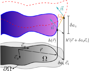
Refer to caption
Figure 1.40: The upper surface, shaded in purple, represents the membrane, while the respective projected surface ΩΩ\Omega is represented by the lower gray shaded surface. The red dashed curve represents the new position of the membrane after deformation.

On one hand, at equilibrium, the energy variation reads

δ=Ωmi[fδai+(fhiifhij)δh+fhijδhj]𝑑s,𝛿subscriptΩsubscript𝑚𝑖delimited-[]𝑓𝛿subscript𝑎𝑖𝑓subscript𝑖subscript𝑖𝑓subscript𝑖𝑗𝛿𝑓subscript𝑖𝑗𝛿subscript𝑗differential-d𝑠\delta\mathcal{H}=\int_{\partial\Omega}m_{i}\left[f\,\delta a_{i}+\left(\frac{\partial f}{\partial h_{i}}-\partial_{i}\frac{\partial f}{\partial h_{ij}}\right)\delta h+\frac{\partial f}{\partial h_{ij}}\delta h_{j}\right]ds\,, (1.53)

where ds𝑑𝑠ds is a length of an infinitesimal element of the curve Ω(x,y)Ω𝑥𝑦\partial\Omega(x,y). On the other hand, we have in terms of the stress tensor

δ=Ωδ𝒂𝚺𝒎𝑑s.𝛿subscriptΩ𝛿𝒂𝚺𝒎differential-d𝑠\delta\mathcal{H}=\int_{\partial\Omega}\delta\bm{a}\cdot\bm{\Sigma}\cdot\bm{m}\,ds\,. (1.54)

One can then obtain 𝚺𝚺\bm{\Sigma} by comparing eq.(1.53) and eq.(1.54). In order to do so, one must express δh𝛿\delta h and δhj𝛿subscript𝑗\delta h_{j} over the boundary in terms of δ𝒂𝛿𝒂\delta\bm{a}. As shown in Fig. 1.40, we have h(𝒓+δai(𝒓)𝒆i)=h(𝒓)+δaz(𝒓)superscript𝒓𝛿subscript𝑎𝑖𝒓subscript𝒆𝑖𝒓𝛿subscript𝑎𝑧𝒓h^{\prime}(\bm{r}+\delta a_{i}(\bm{r})\,\bm{e}_{i})=h(\bm{r})+\delta a_{z}(\bm{r}). Up to first order on δh𝛿\delta h, it is easy to deduce δh=δazδajhj𝛿𝛿subscript𝑎𝑧𝛿subscript𝑎𝑗subscript𝑗\delta h=\delta a_{z}-\delta a_{j}\,h_{j}. Finally, one has to impose that the normal 𝒏𝒏\bm{n} at the boundary is kept constant, which yields hk(𝒓+δai(𝒓)𝒆i)=hk(𝒓)subscriptsuperscript𝑘𝒓𝛿subscript𝑎𝑖𝒓subscript𝒆𝑖subscript𝑘𝒓h^{\prime}_{k}(\bm{r}+\delta a_{i}(\bm{r})\,\bm{e}_{i})=h_{k}(\bm{r}). Again, up to first order, one has kδh=δajhjksubscript𝑘𝛿𝛿subscript𝑎𝑗subscript𝑗𝑘\partial_{k}\delta h=-\delta a_{j}\,h_{jk}. These results put together lead to

ΣijsubscriptΣ𝑖𝑗\displaystyle\Sigma_{ij} =\displaystyle= fδij[fhjk(fhjk)]hifhjkhik,𝑓subscript𝛿𝑖𝑗delimited-[]𝑓subscript𝑗subscript𝑘𝑓subscript𝑗𝑘subscript𝑖𝑓subscript𝑗𝑘subscript𝑖𝑘\displaystyle f\,\delta_{ij}-\left[\frac{\partial f}{\partial h_{j}}-\partial_{k}\left(\frac{\partial f}{\partial h_{jk}}\right)\right]h_{i}-\frac{\partial f}{\partial h_{jk}}h_{ik}\,, (1.55)
ΣzjsubscriptΣ𝑧𝑗\displaystyle\Sigma_{zj} =\displaystyle= fhjk(fhjk).𝑓subscript𝑗subscript𝑘𝑓subscript𝑗𝑘\displaystyle\frac{\partial f}{\partial h_{j}}-\partial_{k}\left(\frac{\partial f}{\partial h_{jk}}\right)\,. (1.56)

In the case of the Helfrich Hamiltonian, one has

f=σ+σ2(h)2+κ2(2h)2+f¯,𝑓𝜎𝜎2superscript2𝜅2superscriptsuperscript22¯𝑓f=\sigma+\frac{\sigma}{2}(\nabla h)^{2}+\frac{\kappa}{2}(\nabla^{2}h)^{2}+\bar{f}\,, (1.57)

where f¯=κGdet(hij)¯𝑓subscript𝜅𝐺𝑑𝑒𝑡subscript𝑖𝑗\bar{f}=\kappa_{G}\,det(h_{ij}) is the contribution from the Gaussian curvature. Eqs.(1.55)-(1.56) become thus

ΣxxsubscriptΣ𝑥𝑥\displaystyle\Sigma_{xx} =\displaystyle= σ+σ2(hy2hx2)+κ2(hyy2hxx2)+κhxx2h,𝜎𝜎2superscriptsubscript𝑦2superscriptsubscript𝑥2𝜅2superscriptsubscript𝑦𝑦2superscriptsubscript𝑥𝑥2𝜅subscript𝑥subscript𝑥superscript2\displaystyle\sigma+\frac{\sigma}{2}\left(h_{y}^{2}-h_{x}^{2}\right)+\frac{\kappa}{2}\left(h_{yy}^{2}-h_{xx}^{2}\right)+\kappa\,h_{x}\partial_{x}\nabla^{2}h\,, (1.58)
ΣxysubscriptΣ𝑥𝑦\displaystyle\Sigma_{xy} =\displaystyle= σhxhyκhxy2h+κhxy2h,𝜎subscript𝑥subscript𝑦𝜅subscript𝑥𝑦superscript2𝜅subscript𝑥subscript𝑦superscript2\displaystyle-\sigma\,h_{x}h_{y}-\kappa\,h_{xy}\nabla^{2}h+\kappa\,h_{x}\partial_{y}\nabla^{2}h\,, (1.59)
ΣzxsubscriptΣ𝑧𝑥\displaystyle\Sigma_{zx} =\displaystyle= σhxκx2h.𝜎subscript𝑥𝜅subscript𝑥superscript2\displaystyle\sigma\,h_{x}-\kappa\,\partial_{x}\nabla^{2}h\,. (1.60)

The other components of the tensor can be obtained by permutation of x𝑥x and y𝑦y. Remark that these expressions are valid up to order two in hh and that the Gaussian curvature gives no contribution to the stress tensor.

Part I Planar membranes

Chapter 2 Planar membrane

As we have seen in the last chapter, membranes are very particular systems from the mechanical point of view: they are liquid, but rigid; they disrupt very easily under stretching and they fluctuate a lot in even in sub-optical levels.

Accordingly, the term surface tension has always been rather confusing. First, it refers to the energy needed to bring a bunch of phospholipids in contact with the aqueous media, which we denote γ𝛾\gamma. As these molecules are amphiphilic, there is almost no energetic cost for creating an interface. Consequently, one can find in the literature statements like “a membrane has vanishing surface tension” [60]. Secondly, the expression stands for the tension τ𝜏\tau that one can mechanically apply to a membrane, for instance, by aspiring it with a micropipette or by extracting a nanotube. As discussed in section 1.2.1, unless in extreme situations, this tension has entropic origin, coming from the flattening of thermal fluctuations. Thus, it is also called effective mechanical tension. At last, surface tension denotes also the multiplier Lagrange σ𝜎\sigma one adds to the Hamiltonian in order to fix the total membrane’s area, as we have done in section 1.3.6. In this case, the tension is more like a chemical potential associated to the total membrane area. The tension σ𝜎\sigma is not experimentally measurable, but its large-scale counterpart r𝑟r, renormalized by fluctuations, is measurable through the q2superscript𝑞2q^{2} dependence of the spectrum fluctuation.

From an experimental point of view, it is fundamental to determine the relation between r𝑟r, σ𝜎\sigma and τ𝜏\tau. In particular, it is very important to determine under which conditions these quantities can be assumed identical. Indeed, experimentally, one measures usually r𝑟r or τ𝜏\tau, whereas the theoretical predictions involve frequently σ𝜎\sigma, which is non measurable. One takes currently for granted the equality between τ𝜏\tau, σ𝜎\sigma and r𝑟r to interpret data, as one can see in the sum-up presented in table 1.1, even though there is no support to this premise.

Many theoretical articles were written in order to clarify this question [2], [68], [104], [3]. In most cases, the authors tried to derive r𝑟r and τ𝜏\tau from the free-energy \mathcal{F}. This route is however very tricky, since one needs to consider terms up to 𝒪(h4)𝒪superscript4\mathcal{O}(h^{4}) in order to evaluate r𝑟r. In this case, the naive measure presented in section 1.3.6 must be subtly corrected [2]. Besides, the definition of the effective mechanical tension τ𝜏\tau from the free-energy is not so clear and slightly different alternatives for the definition presented in eq.(1.7) were proposed.

In this chapter, we try to address the question of the relation between τ𝜏\tau and σ𝜎\sigma for symmetrical planar membranes in contact with a lipid reservoir. We evaluate τ𝜏\tau using the projected stress tensor introduced in the end of the last chapter in section 1.5.2. This calculation is much more straightforward, since one avoids problems related to the choice of the measure. Besides, the definition of τ𝜏\tau in terms of the projected stress tensor is unique: τ𝜏\tau is simply given by the average of the latter. In this section, we show that in general, we can assume τ=σσ0𝜏𝜎subscript𝜎0\tau=\sigma-\sigma_{0}, where σ0subscript𝜎0\sigma_{0} is a constant non negligible for small tensions.

In section 2.2, we compare our result to the ones derived by Cai et al. [2] and by Imparato [3] by differentiating the free-energy with respect to the projected area Apsubscript𝐴𝑝A_{p}. In his derivation, Imparato used the definition presented in eq.(1.7), while Cai et al. used slightly different definition, obtaining consequently a different result. In this section, we show that our result coincides with the one from Imparato, which gives support to the definition presented in the last chapter

τ=(Ap)Np,𝜏subscriptsubscript𝐴𝑝subscript𝑁𝑝\tau=\left(\frac{\partial\mathcal{F}}{\partial A_{p}}\right)_{N_{p}}\,, (2.1)

where the derivative is taken with the total number of lipids constant. Besides, we question the previous demonstration by Cai et al. that τ=r𝜏𝑟\tau=r, since their definition of τ𝜏\tau seems less suitable. We propose then that in general, we should have three different values for τ𝜏\tau, σ𝜎\sigma and r𝑟r. In order to check this prediction, we present a simple numerical experiment in section 2.3.

In section 2.4 and  2.5 we discuss some consequences to experiments, namely to those involving micropipettes, introduced in section 1.4.1. As τ𝜏\tau is indeed different from σ𝜎\sigma, we propose corrections to the eq.(1.36) presented in the last chapter. We conclude in section 2.5 with the description of the first recent numerical and experimental evidences that τσ𝜏𝜎\tau\neq\sigma. All results presented in this chapter were obtained under the direction of Jean-Baptiste Fournier and published in [1].

2.1 Evaluation of 𝝉𝝉{\bm{\tau}} from the stress tensor

Consider a planar membrane whose projected area on a plan ΠΠ\Pi parallel to the average plan of the membrane is Apsubscript𝐴𝑝A_{p} and well described by the Helfrich Hamiltonian given in eq.(1.15). This membrane is not stretched and departs very weakly from a plane. Therefore, we use the Monge’s gauge and develop \mathcal{H} up to order two, obtaining the Hamiltonian given in eq.(1.16), the average |h(𝒒)|2delimited-⟨⟩superscript𝒒2\langle|h(\bm{q})|^{2}\rangle given in eq.(1.29) and the projected stress tensor is given in eqs.(1.58)-(1.60). Consider now a cut of length L𝐿L on ΠΠ\Pi parallel to 𝒆ysubscript𝒆𝑦\bm{e}_{y}, so that the normal to the projected cut is simply 𝒎=𝒆x𝒎subscript𝒆𝑥\bm{m}=\bm{e}_{x}, as shown in Fig. 2.1.

Refer to caption
Figure 2.1: Weakly fluctuating planar membrane described in the Monge’s gauge. The force 𝒇𝒇\bm{f} is exchanged through the cut of projected length L𝐿L (red). Note that we have chosen an orthonormal basis in order to have 𝒎=𝒆x𝒎subscript𝒆𝑥\bm{m}=\bm{e}_{x}.

The force exchanged through the cut is

𝒇=L/2L/2(Σxx𝒆x+Σyx𝒆y+Σzx𝒆z)𝑑y.𝒇superscriptsubscript𝐿2𝐿2subscriptΣ𝑥𝑥subscript𝒆𝑥subscriptΣ𝑦𝑥subscript𝒆𝑦subscriptΣ𝑧𝑥subscript𝒆𝑧differential-d𝑦\bm{f}=\int_{-L/2}^{L/2}\left(\Sigma_{xx}\,\bm{e}_{x}+\Sigma_{yx}\,\bm{e}_{y}+\Sigma_{zx}\,\bm{e}_{z}\right)\,dy\,. (2.2)

The thermal average of 𝒇𝒇\bm{f}, denoted by the brackets \langle\rangle, is given by

𝒇=L(Σxx𝒆x+Σyx𝒆y+Σzx𝒆z).delimited-⟨⟩𝒇𝐿delimited-⟨⟩subscriptΣ𝑥𝑥subscript𝒆𝑥delimited-⟨⟩subscriptΣ𝑦𝑥subscript𝒆𝑦delimited-⟨⟩subscriptΣ𝑧𝑥subscript𝒆𝑧\langle\bm{f}\rangle=L\left(\langle\Sigma_{xx}\rangle\,\bm{e}_{x}+\langle\Sigma_{yx}\rangle\,\bm{e}_{y}+\langle\Sigma_{zx}\rangle\,\bm{e}_{z}\right)\,. (2.3)

One must evaluate the average of each term of eqs.(1.58)-(1.60). Hence, it is interesting to use the Fourier transform introduced in section 1.3.6

h(𝒓)=1Ap𝒒hn,mei𝒒𝒓,𝒓1subscript𝐴𝑝subscript𝒒subscript𝑛𝑚superscript𝑒𝑖𝒒𝒓h(\bm{r})=\frac{1}{\sqrt{A_{p}}}\sum_{\bm{q}}h_{n,m}\,e^{i\,\bm{q}\cdot\bm{r}}\,, (2.4)

with 𝒒=2π/Ap(n,m)𝒒2𝜋subscript𝐴𝑝𝑛𝑚\bm{q}=2\pi/\sqrt{A_{p}}\,(n,m), n,m𝑛𝑚n,m\in\mathbb{N} and

𝒒|n|Nmax|m|Nmax.subscript𝒒subscript𝑛subscript𝑁maxsubscript𝑚subscript𝑁max\sum_{\bm{q}}\equiv\sum_{|n|\,\leq\,N_{\mathrm{max}}}\,\sum_{|m|\,\leq\,N_{\mathrm{max}}}\,. (2.5)

Note that as h(𝒓)𝒓h(\bm{r}) is real, one has hn,m=hn,msubscript𝑛𝑚superscriptsubscript𝑛𝑚h_{-n,-m}=h_{n,m}^{*}, where the symbol indicates the complex conjugate. The mode n=0𝑛0n=0 and m=0𝑚0m=0 corresponds to a simple translation and gives no contribution to the energy. It will be therefore omitted throughout this section.

Using this definition of the Fourier transform, the Hamiltonian for a weakly fluctuating membrane in contact with a lipid reservoir introduced in section 1.3.6 becomes

=σAp+12𝒒(σq2+κq4)|hn,m|2,𝜎subscript𝐴𝑝12subscript𝒒𝜎superscript𝑞2𝜅superscript𝑞4superscriptsubscript𝑛𝑚2\mathcal{H}=\sigma\,A_{p}+\frac{1}{2}\sum_{\bm{q}}\left(\sigma q^{2}+\kappa q^{4}\right)|h_{n,m}|^{2}\,, (2.6)

where q𝑞q varies between qmin=2π/Apsubscript𝑞min2𝜋subscript𝐴𝑝q_{\mathrm{min}}=2\pi/\sqrt{A_{p}} up to Λ=2πNmax/Ap1/aΛ2𝜋subscript𝑁maxsubscript𝐴𝑝1𝑎\Lambda=2\pi N_{\mathrm{max}}/\sqrt{A_{p}}\approx 1/a, where a𝑎a is a microscopical cut-off comparable to the membrane thickness. The correlation function is given by

G(𝒓𝒓)𝐺𝒓superscript𝒓\displaystyle G(\bm{r}-\bm{r}^{\prime}) \displaystyle\equiv h(𝒓)h(𝒓)delimited-⟨⟩𝒓superscript𝒓\displaystyle\langle h(\bm{r})h(\bm{r}^{\prime})\rangle\, (2.7)
=\displaystyle= 1Ap𝒒𝒌hn,mhn,mei𝒒𝒓ei𝒌𝒓1subscript𝐴𝑝subscript𝒒subscript𝒌delimited-⟨⟩subscript𝑛𝑚subscriptsuperscript𝑛superscript𝑚superscript𝑒𝑖𝒒𝒓superscript𝑒𝑖𝒌superscript𝒓bold-′\displaystyle\frac{1}{A_{p}}\sum_{\bm{q}}\sum_{\bm{k}}\langle h_{n,m}h_{n^{\prime},m^{\prime}}\rangle\,e^{i\,\bm{q}\cdot\bm{r}}e^{i\,\bm{k}\cdot\bm{r^{\prime}}}\,
=\displaystyle= kBTAp𝒒ei𝒒(𝒓𝒓)σq2+κq4,subscript𝑘B𝑇subscript𝐴𝑝subscript𝒒superscript𝑒𝑖𝒒𝒓superscript𝒓bold-′𝜎superscript𝑞2𝜅superscript𝑞4\displaystyle\frac{k_{\mathrm{B}}T}{A_{p}}\sum_{\bm{q}}\frac{e^{i\,\bm{q}\cdot(\bm{r}-\bm{r^{\prime}})}}{\sigma\,q^{2}+\kappa\,q^{4}}\,,

where we have used the result displayed on eq.(1.29) to obtain the last passage.

It is a straightforward calculation to evaluate averages using the correlation function. As an example, we do a step-by-step evaluation the average of ΣxxsubscriptΣ𝑥𝑥\Sigma_{xx}:

Σxxdelimited-⟨⟩subscriptΣ𝑥𝑥\displaystyle\langle\Sigma_{xx}\rangle =\displaystyle= σ+κhxhxxx+hxhxyy𝜎𝜅delimited-⟨⟩subscript𝑥subscript𝑥𝑥𝑥subscript𝑥subscript𝑥𝑦𝑦\displaystyle\sigma+\kappa\,\langle h_{x}h_{xxx}+h_{x}h_{xyy}\rangle\, (2.8)
=\displaystyle= σ+κxx(x2+y2)G(𝒓𝒓)|𝒓=𝒓𝜎evaluated-at𝜅subscript𝑥subscriptsuperscript𝑥superscriptsubscriptsuperscript𝑥2superscriptsubscriptsuperscript𝑦2𝐺𝒓superscript𝒓bold-′𝒓superscript𝒓\displaystyle\sigma+\kappa\,\partial_{x}\partial_{x^{\prime}}\left(\partial_{x^{\prime}}^{2}+\partial_{y^{\prime}}^{2}\right)G\left(\bm{r}-\bm{r^{\prime}}\right)|_{\bm{r}=\bm{r}^{\prime}}
=\displaystyle= σ+κkBTAp𝒒(iqx)(iqx)(qx2qy2)σq2+κq4𝜎𝜅subscript𝑘B𝑇subscript𝐴𝑝subscript𝒒𝑖subscript𝑞𝑥𝑖subscript𝑞𝑥superscriptsubscript𝑞𝑥2superscriptsubscript𝑞𝑦2𝜎superscript𝑞2𝜅superscript𝑞4\displaystyle\sigma+\kappa\,\frac{k_{\mathrm{B}}T}{A_{p}}\,\sum_{\bm{q}}\frac{(i\,q_{x})(-i\,q_{x})\left(-q_{x}^{2}-q_{y}^{2}\right)}{\sigma\,q^{2}+\kappa\,q^{4}}
=\displaystyle= σkBTAp𝒒κqx2σ+κq2𝜎subscript𝑘B𝑇subscript𝐴𝑝subscript𝒒𝜅superscriptsubscript𝑞𝑥2𝜎𝜅superscript𝑞2\displaystyle\sigma-\frac{k_{\mathrm{B}}T}{A_{p}}\sum_{\bm{q}}\frac{\kappa\,q_{x}^{2}}{\sigma+\kappa\,q^{2}}
=\displaystyle= σkBT2Ap𝒒κq2σ+κq2,𝜎subscript𝑘B𝑇2subscript𝐴𝑝subscript𝒒𝜅superscript𝑞2𝜎𝜅superscript𝑞2\displaystyle\sigma-\frac{k_{\mathrm{B}}T}{2A_{p}}\sum_{\bm{q}}\frac{\kappa\,q^{2}}{\sigma+\kappa\,q^{2}}\,,

where we used in the first and in the last passage the fact that by symmetry hx2=hy2delimited-⟨⟩superscriptsubscript𝑥2delimited-⟨⟩superscriptsubscript𝑦2\langle h_{x}^{2}\rangle=\langle h_{y}^{2}\rangle and hxx2=hyy2delimited-⟨⟩superscriptsubscript𝑥𝑥2delimited-⟨⟩superscriptsubscript𝑦𝑦2\langle h_{xx}^{2}\rangle=\langle h_{yy}^{2}\rangle. By the same reasoning, one can demonstrate that Σyx=0delimited-⟨⟩subscriptΣ𝑦𝑥0\langle\Sigma_{yx}\rangle=0 and Σzx=0delimited-⟨⟩subscriptΣ𝑧𝑥0\langle\Sigma_{zx}\rangle=0, as expected given the symmetry of the system. We have thus the effective tension τ𝜏\tau, which relates to the average of the force 𝒇𝒇\bm{f} through

τ𝒇𝒆xL=σkBT2Ap𝒒κq2σ+κq2.𝜏delimited-⟨⟩𝒇subscript𝒆𝑥𝐿𝜎subscript𝑘B𝑇2subscript𝐴𝑝subscript𝒒𝜅superscript𝑞2𝜎𝜅superscript𝑞2\tau\equiv\frac{\langle\bm{f}\rangle\cdot\bm{e}_{x}}{L}=\sigma-\frac{k_{\mathrm{B}}T}{2A_{p}}\sum_{\bm{q}}\frac{\kappa\,q^{2}}{\sigma+\kappa\,q^{2}}\,. (2.9)

In the thermodynamic limit, Apsubscript𝐴𝑝A_{p} is very large and the sum over 𝒒𝒒\bm{q} becomes an integral whose calculation leads to

τσ=kBTΛ28π[1σσrln(1+σrσ)],𝜏𝜎subscript𝑘B𝑇superscriptΛ28𝜋delimited-[]1𝜎subscript𝜎𝑟1subscript𝜎𝑟𝜎\tau-\sigma=-\frac{k_{\mathrm{B}}T\,\Lambda^{2}}{8\pi}\left[1-\frac{\sigma}{\sigma_{r}}\ln\left(1+\frac{\sigma_{r}}{\sigma}\right)\right]\,, (2.10)

where σr=κΛ2subscript𝜎𝑟𝜅superscriptΛ2\sigma_{r}=\kappa\Lambda^{2}. Numerically, for typical values a5nm𝑎5nma\approx 5\,\mathrm{nm} and κ1019J𝜅superscript1019J\kappa\approx 10^{-19}\,\mathrm{J}, one obtains σr5×103N/msubscript𝜎𝑟5superscript103Nm\sigma_{r}\approx 5\times 10^{-3}\,\mathrm{N/m}, which is of the same order of magnitude of the rupture tension of membranes [55]. Fig. 2.2 shows the difference στ𝜎𝜏\sigma-\tau normalized by

σ0=kBTΛ28π=σr8πβκ,subscript𝜎0subscript𝑘B𝑇superscriptΛ28𝜋subscript𝜎𝑟8𝜋𝛽𝜅\sigma_{0}=\frac{k_{\mathrm{B}}T\,\Lambda^{2}}{8\pi}=\frac{\sigma_{r}}{8\pi\beta\kappa}\,, (2.11)

as a function of σ/σr𝜎subscript𝜎𝑟\sigma/\sigma_{r}.

Refer to caption
Figure 2.2: The difference στ𝜎𝜏\sigma-\tau normalized by σ0subscript𝜎0\sigma_{0} as a function σ/σr𝜎subscript𝜎𝑟\sigma/\sigma_{r}. For tensions smaller than 102σrsuperscript102subscript𝜎𝑟10^{-2}\,\sigma_{r}, we see that τσσ0similar-to-or-equals𝜏𝜎subscript𝜎0\tau\simeq\sigma-\sigma_{0}. The green shaded area corresponds to the region where we expect our theory to need corrections due to the stretching of the membrane.

As we can see, it is a good approximation to set τσσ0similar-to-or-equals𝜏𝜎subscript𝜎0\tau\simeq\sigma-\sigma_{0} for σ<102σr𝜎superscript102subscript𝜎𝑟\sigma<10^{-2}\,\sigma_{r}. Beyond this limit, the tension is relatively high and we expect corrections coming from the stretching of the membrane. For the previous values of a𝑎a and κ𝜅\kappa and taking kBT4×1021Jsubscript𝑘B𝑇4superscript1021Jk_{\mathrm{B}}T\approx 4\times 10^{-21}\,\mathrm{J}, we obtain σ05×106N/msubscript𝜎05superscript106Nm\sigma_{0}\approx 5\times 10^{-6}\,\mathrm{N/m}. As tensions as small as τ108N/m𝜏superscript108Nm\tau\approx 10^{-8}\,\mathrm{N/m} are measured in micropipette experiments, this correction may be non negligible (see Fig. 2.3). We will discuss the consequences of this prediction to experiments in section 2.4.
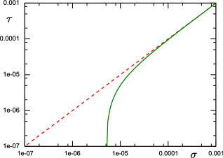
Refer to caption
Figure 2.3: The red dashed straight line shows the standard approximation τσ𝜏𝜎\tau\approx\sigma, while the green curve shows the behavior of τ𝜏\tau predicted by our theory. For small tensions, the correction is relevant. Curves for a=5nm𝑎5nma=5\,\mathrm{nm}, κ=1019J𝜅superscript1019J\kappa=10^{-19}\,\mathrm{J} and kBT=4×10²¹Jsubscript𝑘B𝑇4superscript1021Jk_{\mathrm{B}}T=4\times 10^{-21}\,\mathrm{J}.

2.2 Derivation from the free-energy

Here we re-derive the result given in eq.(2.10) by differentiating the free-energy. To begin, we evaluate the free-energy as in references [2] and [3]. By definition, we have

=kBTln(𝒵),subscript𝑘B𝑇𝒵\mathcal{F}=-k_{\mathrm{B}}T\ln(\mathcal{Z})\,, (2.12)

where 𝒵𝒵\mathcal{Z} is the partition function given by

𝒵=𝒟[h]eβ[h].𝒵𝒟delimited-[]superscript𝑒𝛽delimited-[]\mathcal{Z}=\int\mathcal{D}[h]\,e^{-\beta\mathcal{H}[h]}\,. (2.13)

As discussed in section 1.3.6, one needs a measure to evaluate this integral. We will consider here the naive measure, which is justified up to first order on the temperature and up to second order on hh (further discussion on the subtleties of the measure can be found in [2] and [105]). We discretize the projected plane ΠΠ\Pi in N2superscript𝑁2N^{2} squares of area a¯2superscript¯𝑎2\bar{a}^{2}, so that the height of each one of these squares is denoted hpx,pyh(pxa¯𝒆x+pya¯𝒆y)superscriptsubscript𝑝𝑥subscript𝑝𝑦subscript𝑝𝑥¯𝑎subscript𝒆𝑥subscript𝑝𝑦¯𝑎subscript𝒆𝑦h^{p_{x},p_{y}}\equiv h(p_{x}\,\bar{a}\,\bm{e}_{x}+p_{y}\,\bar{a}\,\bm{e}_{y}). The naive measure reads

𝒟naive[h]=px=1Npy=1Ndhpx,pyλsubscript𝒟naivedelimited-[]superscriptsubscriptproductsubscript𝑝𝑥1𝑁superscriptsubscriptproductsubscript𝑝𝑦1𝑁𝑑superscriptsubscript𝑝𝑥subscript𝑝𝑦𝜆\mathcal{D}_{\mathrm{naive}}[h]=\prod_{p_{x}=1}^{N}\prod_{p_{y}=1}^{N}\frac{dh^{p_{x},p_{y}}}{\lambda}\, (2.14)

The factor λ𝜆\lambda is a vertical quantum introduced to keep 𝒵𝒵\mathcal{Z} dimensionless.

2.2.1 Naive measure in the Fourier space

In section 1.3.6, we have used this measure to evaluate averages, but we have not derived explicitly \mathcal{F}. Here, to do so, we prefer to work in the Fourier space. We need thus to derive the equivalent of the measure above in this space. As in the last section, let’s consider the Fourier transform

hpx,py=1Ap𝒒hn,me2πinpxNe2πimpyNsuperscriptsubscript𝑝𝑥subscript𝑝𝑦1subscript𝐴𝑝subscript𝒒subscript𝑛𝑚superscript𝑒2𝜋𝑖𝑛subscript𝑝𝑥𝑁superscript𝑒2𝜋𝑖𝑚subscript𝑝𝑦𝑁h^{p_{x},p_{y}}=\frac{1}{\sqrt{A_{p}}}\sum_{\bm{q}}h_{n,m}e^{\frac{2\pi in\,p_{x}}{N}}\,e^{\frac{2\pi im\,p_{y}}{N}} (2.15)

Remark that only half of the total number of modes are independent, since hn,m=hn,msubscript𝑛𝑚superscriptsubscript𝑛𝑚h_{-n,-m}=h_{n,m}^{*}. In terms of these independent modes, the measure is thus

𝒟naive[h]=(|n|N2,n 0m=0N2dhn,mλdhn,mλ)×Jsubscript𝒟naivedelimited-[]subscriptproductformulae-sequence𝑛𝑁2𝑛 0superscriptsubscriptproduct𝑚0𝑁2𝑑superscriptsubscript𝑛𝑚𝜆𝑑superscriptsubscript𝑛𝑚𝜆𝐽\mathcal{D}_{\mathrm{naive}}[h]=\left(\prod_{|n|\,\leq\,\frac{N}{2},\,n\,\neq\,0}\,\prod_{m=0}^{\frac{N}{2}}\int\frac{dh_{n,m}^{\mathcal{R}}}{\lambda}\,\frac{dh_{n,m}^{\mathcal{I}}}{\lambda}\right)\times J\, (2.16)

where the superscripts \mathcal{R} and \mathcal{I} stand, respectively, for the real and imaginary part of hn,msubscript𝑛𝑚h_{n,m} and J𝐽J is the Jacobian of the transformation. To simplify notations, in the following we will simply denote

nm0subscriptproduct𝑛subscriptproduct𝑚0\displaystyle\prod_{n}\prod_{m\geq 0} \displaystyle\equiv |n|N2,n 0m=0N2,subscriptproductformulae-sequence𝑛𝑁2𝑛 0superscriptsubscriptproduct𝑚0𝑁2\displaystyle\prod_{|n|\,\leq\,\frac{N}{2},\,n\,\neq\,0}\,\prod_{m=0}^{\frac{N}{2}}\,, (2.17)
nm0subscript𝑛subscript𝑚0\displaystyle\sum_{n}\sum_{m\geq 0} \displaystyle\equiv |n|N2,n 0m=0N2.subscriptformulae-sequence𝑛𝑁2𝑛 0superscriptsubscript𝑚0𝑁2\displaystyle\sum_{|n|\,\leq\,\frac{N}{2},\,n\,\neq\,0}\,\sum_{m=0}^{\frac{N}{2}}\,. (2.18)

To determine J𝐽J, we will evaluate the partition function for a simple Gaussian Hamiltonian. With the measure given in eq.(2.14), we have

𝒵=px=1Npy=1Ndhpx,pyλeαpx=1Npy=1N(hpx,py)2=(πα)N2𝒵superscriptsubscriptproductsubscript𝑝𝑥1𝑁superscriptsubscriptproductsubscript𝑝𝑦1𝑁𝑑superscriptsubscript𝑝𝑥subscript𝑝𝑦𝜆superscript𝑒𝛼superscriptsubscriptsubscript𝑝𝑥1𝑁superscriptsubscriptsubscript𝑝𝑦1𝑁superscriptsuperscriptsubscript𝑝𝑥subscript𝑝𝑦2superscript𝜋𝛼superscript𝑁2\mathcal{Z}=\int\prod_{p_{x}=1}^{N}\prod_{p_{y}=1}^{N}\frac{dh^{p_{x},p_{y}}}{\lambda}\,e^{-\alpha\sum_{p_{x}=1}^{N}\sum_{p_{y}=1}^{N}\,{(h^{p_{x},p_{y}}})^{2}}=\left(\sqrt{\frac{\pi}{\alpha}}\right)^{N^{2}} (2.19)

Using the definition presented in eq.(2.15), the quadratic Hamiltonian becomes

αpx=1Npy=1N(hpx,py)2𝛼superscriptsubscriptsubscript𝑝𝑥1𝑁superscriptsubscriptsubscript𝑝𝑦1𝑁superscriptsuperscriptsubscript𝑝𝑥subscript𝑝𝑦2\displaystyle\alpha\sum_{p_{x}=1}^{N}\sum_{p_{y}=1}^{N}{(h^{p_{x},p_{y}})}^{2} =\displaystyle= αL2𝒒𝒒hn,mhn,m×N2δn,nδm,m𝛼superscript𝐿2subscript𝒒subscriptsuperscript𝒒subscript𝑛𝑚subscriptsuperscript𝑛superscript𝑚superscript𝑁2subscript𝛿superscript𝑛𝑛subscript𝛿superscript𝑚𝑚\displaystyle\frac{\alpha}{L^{2}}\sum_{\bm{q}}\sum_{\bm{q}^{\prime}}h_{n,m}\,h_{n^{\prime},m^{\prime}}\times N^{2}\,\delta_{n^{\prime},-n}\,\delta_{m^{\prime},-m} (2.20)
=\displaystyle= αa¯2𝒒[(hn,m)2+(hn,m)2]𝛼superscript¯𝑎2subscript𝒒delimited-[]superscriptsuperscriptsubscript𝑛𝑚2superscriptsuperscriptsubscript𝑛𝑚2\displaystyle\frac{\alpha}{\bar{a}^{2}}\sum_{\bm{q}}\left[(h_{n,m}^{\mathcal{R}})^{2}+(h_{n,m}^{\mathcal{I}})^{2}\right]

and the partition function is

𝒵=J×nm0dhn,mλdhn,mλeαa¯2𝒒[(hn,m)2+(hn,m)2]=(πa¯2α)N2×J𝒵𝐽subscriptproduct𝑛subscriptproduct𝑚0𝑑superscriptsubscript𝑛𝑚𝜆𝑑superscriptsubscript𝑛𝑚𝜆superscript𝑒𝛼superscript¯𝑎2subscript𝒒delimited-[]superscriptsuperscriptsubscript𝑛𝑚2superscriptsuperscriptsubscript𝑛𝑚2superscript𝜋superscript¯𝑎2𝛼superscript𝑁2𝐽\mathcal{Z}=J\times\int\prod_{n}\,\prod_{m\geq 0}\int\frac{dh_{n,m}^{\mathcal{R}}}{\lambda}\,\frac{dh_{n,m}^{\mathcal{I}}}{\lambda}\,e^{-\frac{\alpha}{\bar{a}^{2}}\sum_{\bm{q}}\left[(h_{n,m}^{\mathcal{R}})^{2}+(h_{n,m}^{\mathcal{I}})^{2}\right]}=\left(\sqrt{\frac{\pi\,\bar{a}^{2}}{\alpha}}\right)^{N^{2}}\times J (2.21)

The partition function should be the same in both eq.(2.19) and eq.(2.21), which implies J=1/(a¯)N2𝐽1superscript¯𝑎superscript𝑁2J=1/(\bar{a})^{N^{2}}. Summing up, in the Fourier space, for a weakly fluctuating membrane, the naive measure is equivalent to

𝒟naive[h]=nm0dhn,mλa¯dhn,mλa¯.subscript𝒟naivedelimited-[]subscriptproduct𝑛subscriptproduct𝑚0𝑑superscriptsubscript𝑛𝑚𝜆¯𝑎𝑑superscriptsubscript𝑛𝑚𝜆¯𝑎\mathcal{D}_{\mathrm{naive}}[h]=\prod_{n}\,\prod_{m\geq 0}\frac{dh_{n,m}^{\mathcal{R}}}{\lambda\bar{a}}\frac{dh_{n,m}^{\mathcal{I}}}{\lambda\bar{a}}\,. (2.22)
2.2.2 Evaluation of 𝓕𝓕\bm{\mathcal{F}} and discussion

Using the Hamiltonian given in eq.(2.6), the partition function given in eq.(2.13) with the measure (2.22) becomes

𝒵𝒵\displaystyle\mathcal{Z} similar-to-or-equals\displaystyle\simeq nm0dhn,mλa¯dhn,mλa¯eβ({hn,m}),subscriptproduct𝑛subscriptproduct𝑚0𝑑superscriptsubscript𝑛𝑚𝜆¯𝑎𝑑superscriptsubscript𝑛𝑚𝜆¯𝑎superscript𝑒𝛽subscript𝑛𝑚\displaystyle\prod_{n}\,\prod_{m\geq 0}\int\frac{dh_{n,m}^{\mathcal{R}}}{\lambda\bar{a}}\frac{dh_{n,m}^{\mathcal{I}}}{\lambda\bar{a}}\,e^{-\beta\mathcal{H}(\{h_{n,m}\})}\,, (2.23)
similar-to-or-equals\displaystyle\simeq eβσApnm0(dhn,mλa¯eβ2nm0(σq2+κq4)hn,m2)superscript𝑒𝛽𝜎subscript𝐴𝑝subscriptproduct𝑛subscriptproduct𝑚0𝑑superscriptsubscript𝑛𝑚𝜆¯𝑎superscript𝑒𝛽2subscript𝑛subscript𝑚0𝜎superscript𝑞2𝜅superscript𝑞4superscriptsuperscriptsubscript𝑛𝑚2\displaystyle e^{-\beta\sigma A_{p}}\prod_{n}\,\prod_{m\geq 0}\left(\int\frac{dh_{n,m}^{\mathcal{R}}}{\lambda\bar{a}}\,e^{-\frac{\beta}{2}\sum_{n}\sum_{m\geq 0}\left(\sigma q^{2}+\kappa q^{4}\right)\,{h_{n,m}^{\mathcal{R}}}^{2}}\right)
×\displaystyle\times (dhn,mλa¯eβ2nm0(σq2+κq4)hn,m2).𝑑superscriptsubscript𝑛𝑚𝜆¯𝑎superscript𝑒𝛽2subscript𝑛subscript𝑚0𝜎superscript𝑞2𝜅superscript𝑞4superscriptsuperscriptsubscript𝑛𝑚2\displaystyle\left(\frac{dh_{n,m}^{\mathcal{I}}}{\lambda\bar{a}}\,e^{-\frac{\beta}{2}\sum_{n}\sum_{m\geq 0}\left(\sigma q^{2}+\kappa q^{4}\right)\,{h_{n,m}^{\mathcal{I}}}^{2}}\right)\,.

Finally, carrying out the Gaussian integrals, we have

𝒵eβσApnm02πβa¯2λ2(σq2+κq4).similar-to-or-equals𝒵superscript𝑒𝛽𝜎subscript𝐴𝑝subscriptproduct𝑛subscriptproduct𝑚02𝜋𝛽superscript¯𝑎2superscript𝜆2𝜎superscript𝑞2𝜅superscript𝑞4\mathcal{Z}\simeq e^{-\beta\sigma A_{p}}\prod_{n}\,\prod_{m\geq 0}\frac{2\pi}{\beta\bar{a}^{2}\lambda^{2}\left(\sigma q^{2}+\kappa q^{4}\right)}\,. (2.24)

Accordingly, the free-energy is given, to lowest order in T𝑇T, by

=σAp+kBTnm0ln[(σq2+κq4)a¯2λ22πkBT],𝜎subscript𝐴𝑝subscript𝑘B𝑇subscript𝑛subscript𝑚0𝜎superscript𝑞2𝜅superscript𝑞4superscript¯𝑎2superscript𝜆22𝜋subscript𝑘B𝑇\mathcal{F}=\sigma\,A_{p}+k_{\mathrm{B}}T\sum_{n}\,\sum_{m\geq 0}\ln\left[\left(\sigma\,q^{2}+\kappa\,q^{4}\right)\frac{\bar{a}^{2}\lambda^{2}}{2\pi k_{\mathrm{B}}T}\right]\,, (2.25)

where we remind that λ𝜆\lambda is a quantum discretizing the membrane vertical displacements. Equivalently, highlighting the dependence of \mathcal{F} on Apsubscript𝐴𝑝A_{p}, one obtains

=σAp+kBTnm0ln[(σq~2+κq~4Ap)λ22πNkBT],𝜎subscript𝐴𝑝subscript𝑘B𝑇subscript𝑛subscript𝑚0𝜎superscript~𝑞2𝜅superscript~𝑞4subscript𝐴𝑝superscript𝜆22𝜋𝑁subscript𝑘B𝑇\mathcal{F}=\sigma\,A_{p}+k_{\mathrm{B}}T\sum_{n}\,\sum_{m\geq 0}\ln\left[\left(\sigma\,\tilde{q}^{2}+\frac{\kappa\,\tilde{q}^{4}}{A_{p}}\right)\frac{\lambda^{2}}{2\pi Nk_{\mathrm{B}}T}\right]\,, (2.26)

where we have used a¯2=Ap/N=4π/Λ2superscript¯𝑎2subscript𝐴𝑝𝑁4𝜋superscriptΛ2\bar{a}^{2}=A_{p}/N=4\pi/\Lambda^{2}, N𝑁N being the total number of modes or degrees of freedom, and 𝒒~=2π(n,m)~𝒒2𝜋𝑛𝑚\tilde{\bm{q}}=2\pi(n,m).

With the definition presented in section 1.2.1

τ=(Ap)Np,𝜏subscriptsubscript𝐴𝑝subscript𝑁𝑝\tau=\left(\frac{\partial\mathcal{F}}{\partial A_{p}}\right)_{N_{p}}\,, (2.27)

one obtains from eq.(2.26)

(Ap)Npsubscriptsubscript𝐴𝑝subscript𝑁𝑝\displaystyle\left(\frac{\partial\mathcal{F}}{\partial A_{p}}\right)_{N_{p}} =\displaystyle= σkBT2Ap𝒒κq2σ+κq2,𝜎subscript𝑘B𝑇2subscript𝐴𝑝subscript𝒒𝜅superscript𝑞2𝜎𝜅superscript𝑞2\displaystyle\sigma-\frac{k_{\mathrm{B}}T}{2A_{p}}\sum_{\bm{q}}\frac{\kappa\,q^{2}}{\sigma+\kappa q^{2}}\,, (2.28)

where the derivation was taken keeping the number of modes constant. Indeed, once the cutoff ΛΛ\Lambda is fixed, having a total number of particles fixed is equivalent to having a total number of modes fixed. This result coincides with our previous derivation (eq.(2.10)) and gives some evidence of the correctness of the derivation presented in [3]. Instead, in their work, Cai et al. used a slightly different definition for the effective tension, assuming

τCai=limAp,subscript𝜏Caisubscriptlimsubscript𝐴𝑝\tau_{\mathrm{Cai}}=\frac{\partial\mathcal{F_{\mathrm{lim}}}}{\partial A_{p}}\,, (2.29)

where limsubscriptlim\mathcal{F}_{\mathrm{lim}} is the free-energy in the limit of very large membranes. In this case, the sum in eq.(2.25) becomes an integral and one obtains

lim=σAp+kBTAp2d2q(2π)2ln[(σq2+κq4)a¯2λ22πkBT].subscriptlim𝜎subscript𝐴𝑝subscript𝑘B𝑇subscript𝐴𝑝2superscript𝑑2𝑞superscript2𝜋2𝜎superscript𝑞2𝜅superscript𝑞4superscript¯𝑎2superscript𝜆22𝜋subscript𝑘B𝑇\mathcal{F}_{\mathrm{lim}}=\sigma\,A_{p}+\frac{k_{\mathrm{B}}T\,A_{p}}{2}\int\frac{d^{2}q}{(2\pi)^{2}}\ln\left[\left(\sigma q^{2}+\kappa q^{4}\right)\frac{\bar{a}^{2}\lambda^{2}}{2\pi k_{\mathrm{B}}T}\right]\,. (2.30)

It follows

limAp=σ+kBT2d2q(2π)2ln[(σq2+κq4)a¯2λ22πkBT].subscriptlimsubscript𝐴𝑝𝜎subscript𝑘B𝑇2superscript𝑑2𝑞superscript2𝜋2𝜎superscript𝑞2𝜅superscript𝑞4superscript¯𝑎2superscript𝜆22𝜋subscript𝑘B𝑇\frac{\partial\mathcal{F}_{\mathrm{lim}}}{\partial A_{p}}=\sigma+\frac{k_{\mathrm{B}}T}{2}\int\frac{d^{2}q}{(2\pi)^{2}}\ln\left[\left(\sigma q^{2}+\kappa q^{4}\right)\frac{\bar{a}^{2}\lambda^{2}}{2\pi k_{\mathrm{B}}T}\right]\,. (2.31)

As this result disagrees with the one obtained in eq.(2.10), we conclude that the definition eq.(2.27) is more appropriate: one must first differentiate with respect to Apsubscript𝐴𝑝A_{p} keeping the number of modes constant and only after take the thermodynamic limit, if needed. Note that with the projected stress tensor these subtleties are avoided, once one deals only with the straightforward evaluation of averages.

2.2.3 What about r?

In their work, Cai et al. showed also that one should have r=τ𝑟𝜏r=\tau. Here we will present in detail their reasoning and argue that their conclusion follow from the fact that their definition of τ𝜏\tau is slightly different from ours (compare eq.(2.31) with the thermodynamical limit of eq.(2.28)). Thus, in general, one should have rτ𝑟𝜏r\neq\tau.

First of all, as in section 1.3.6, they introduced a conjugated field m(𝒓)𝑚𝒓m(\bm{r}) to the Hamiltonian in order to fix a general average shape h(𝒓)=h¯(𝒓)h¯delimited-⟨⟩𝒓¯𝒓¯\langle h(\bm{r})\rangle=\bar{h}(\bm{r})\equiv\bar{h}, obtaining

=Sh(𝒓)m(𝒓)𝑑A,superscriptsubscript𝑆𝒓𝑚𝒓differential-d𝐴\mathcal{H}^{\prime}=\mathcal{H}-\int_{S}h(\bm{r})\,m(\bm{r})\,dA\,, (2.32)

where \mathcal{H} is the physical Hamiltonian given in eq.(1.15). The corresponding partition function is

𝒵=𝒟[h]eβ[h]eβShm𝑑A𝒵𝒟delimited-[]superscript𝑒𝛽delimited-[]superscript𝑒𝛽subscript𝑆𝑚differential-d𝐴\mathcal{Z}=\int\mathcal{D}[h]\,e^{-\beta\mathcal{H}[h]}\,e^{\beta\int_{S}h\,m\,dA} (2.33)

and the effective action, i. e., the Legendre transform of the free-energy, is given by

eff=kBTln𝒵+Sh¯m𝑑A.subscripteffsubscript𝑘B𝑇𝒵subscript𝑆¯𝑚differential-d𝐴\mathcal{F}_{\mathrm{eff}}=-k_{\mathrm{B}}T\ln\mathcal{Z}+\int_{S}\bar{h}\,m\,dA\,. (2.34)

The average height of the membrane is given by

h(𝒓)m𝒟[h]h(𝒓)eβ[h]eShm𝑑A𝒵=kBT𝒵δ𝒵δm(𝒓)=h¯(𝒓),subscriptdelimited-⟨⟩𝒓𝑚𝒟delimited-[]𝒓superscript𝑒𝛽delimited-[]superscript𝑒subscript𝑆𝑚differential-d𝐴𝒵subscript𝑘B𝑇𝒵𝛿𝒵𝛿𝑚𝒓¯𝒓\displaystyle\langle h(\bm{r})\rangle_{m}\equiv\frac{\int\mathcal{D}[h]\,h(\bm{r})\,e^{-\beta\mathcal{H}[h]}\,e^{\int_{S}h\,m\,dA}}{\mathcal{Z}}=\frac{k_{\mathrm{B}}T}{\mathcal{Z}}\frac{\delta\mathcal{Z}}{\delta m(\bm{r})}=\bar{h}(\bm{r})\,, (2.35)

where δ𝒵/δm(𝒓)𝛿𝒵𝛿𝑚𝒓\delta\mathcal{Z}/\delta m(\bm{r}) stands for the functional derivative of the effective partition function with respect to the field m𝑚m at the point 𝒓𝒓\bm{r}. For m=0𝑚0m=0, we have a simple Gaussian integral and thus h¯(𝒓)|m=0=0evaluated-at¯𝒓𝑚00\bar{h}(\bm{r})|_{m=0}=0, which corresponds to the case of a planar membrane. Differentiating the free-energy with respect to h¯(𝒓)¯𝒓\bar{h}(\bm{r}) and using eq.(2.35), one obtains

δeffδh¯(𝒓)=m(𝒓)kBT𝒵δm(𝒓)δh¯(𝒓)δ𝒵δm(𝒓)𝑑A+δm(𝒓)δh¯(𝒓)h¯(𝒓)𝑑A=m(𝒓).𝛿subscripteff𝛿¯𝒓𝑚𝒓subscript𝑘B𝑇𝒵𝛿𝑚superscript𝒓𝛿¯𝒓𝛿𝒵𝛿𝑚superscript𝒓differential-d𝐴𝛿𝑚superscript𝒓𝛿¯𝒓¯superscript𝒓differential-d𝐴𝑚𝒓\frac{\delta\mathcal{F}_{\mathrm{eff}}}{\delta\bar{h}(\bm{r})}=m(\bm{r})-\frac{k_{\mathrm{B}}T}{\mathcal{Z}}\int\frac{\delta m(\bm{r}^{\prime})}{\delta\bar{h}(\bm{r})}\,\frac{\delta\mathcal{Z}}{\delta m(\bm{r}^{\prime})}\,dA+\int\frac{\delta m(\bm{r}^{\prime})}{\delta\bar{h}(\bm{r})}\,\bar{h}(\bm{r}^{\prime})\,dA=m(\bm{r})\,. (2.36)

For the case m=0𝑚0m=0, the correlation function is given by

h(𝒓)h(𝒓)m=0subscriptdelimited-⟨⟩𝒓superscript𝒓𝑚0\displaystyle\langle h(\bm{r})\,h(\bm{r}^{\prime})\rangle_{m=0} =\displaystyle= (kBT)2𝒵δ2𝒵δm(𝒓)δm(𝒓)|0,evaluated-atsuperscriptsubscript𝑘B𝑇2𝒵superscript𝛿2𝒵𝛿𝑚𝒓𝛿𝑚superscript𝒓0\displaystyle\frac{(k_{\mathrm{B}}T)^{2}}{\mathcal{Z}}\,\left.\frac{\delta^{2}\mathcal{Z}}{\delta m(\bm{r})\delta m(\bm{r}^{\prime})}\right|_{0}\,, (2.37)
=\displaystyle= kBT𝒵δ[𝒵h¯(𝒓)]δm(𝒓)|0,evaluated-atsubscript𝑘B𝑇𝒵𝛿delimited-[]𝒵¯superscript𝒓𝛿𝑚𝒓0\displaystyle\frac{k_{\mathrm{B}}T}{\mathcal{Z}}\,\left.\frac{\delta\left[\mathcal{Z}\,\bar{h}(\bm{r}^{\prime})\right]}{\delta m(\bm{r})}\right|_{0}\,,
=\displaystyle= kBT[δm(𝒓)δh¯(𝒓)|0]1,subscript𝑘B𝑇superscriptdelimited-[]evaluated-at𝛿𝑚𝒓𝛿¯superscript𝒓01\displaystyle k_{\mathrm{B}}T\left[\left.\frac{\delta m(\bm{r})}{\delta\bar{h}(\bm{r}^{\prime})}\right|_{0}\right]^{-1}\,,
=\displaystyle= kBT[δeffδh¯(𝒓)δh¯(𝒓)|0]1,subscript𝑘B𝑇superscriptdelimited-[]evaluated-at𝛿subscripteff𝛿¯𝒓𝛿¯superscript𝒓01\displaystyle k_{\mathrm{B}}T\left[\left.\frac{\delta\mathcal{F}_{\mathrm{eff}}}{\delta\bar{h}(\bm{r})\,\delta\bar{h}(\bm{r}^{\prime})}\right|_{0}\right]^{-1}\,,

where we have used eq.(2.35) and eq.(2.36) in the second and third passage, respectively.

Meanwhile, as we have seen above, Cai et al. defined the tension as

τCai=limAp=eff,lim[h¯=0]Ap,subscript𝜏Caisubscriptlimsubscript𝐴𝑝subscriptefflimdelimited-[]¯0subscript𝐴𝑝\tau_{\mathrm{Cai}}=\frac{\partial\mathcal{F}_{\mathrm{lim}}}{\partial A_{p}}=\frac{\partial\mathcal{F}_{\mathrm{eff,lim}}\,[\bar{h}=0]}{\partial A_{p}}\,, (2.38)

where the eff,limsubscriptefflim\mathcal{F}_{\mathrm{eff,lim}} is the effective action for the limit of large membranes. Suppose now that the average shape h¯(𝒓)¯𝒓\bar{h}(\bm{r}) is tilted. The free-energy should remain the same, since the physical area of the membrane has not changed. The dependence of the free-energy on h¯¯\bar{h} to lowest order should thus be[105]

eff=τCaiS[(1+12(h¯)2+)+]𝑑A,subscripteffsubscript𝜏Caisubscript𝑆delimited-[]112superscript¯2differential-d𝐴\mathcal{F}_{\mathrm{eff}}=\tau_{\mathrm{Cai}}\int_{S}\left[\left(1+\frac{1}{2}(\vec{\nabla}\bar{h})^{2}+\cdots\right)+\cdots\right]\,dA\,, (2.39)

where the first ellipsis involves terms 𝒪(h¯4)𝒪superscript¯4\mathcal{O}(\bar{h}^{4}) and the second involves high order derivatives on h¯¯\bar{h}. Note that the dependence should remain the same if one takes the thermodynamical limit. One has thus

δeffδh¯(𝒓)δh¯(𝒓)|m=0=τCaiΔ𝒓δ(𝒓𝒓)+.evaluated-at𝛿subscripteff𝛿¯𝒓𝛿¯superscript𝒓𝑚0subscript𝜏CaisubscriptΔ𝒓𝛿𝒓superscript𝒓\left.\frac{\delta\mathcal{F}_{\mathrm{eff}}}{\delta\bar{h}(\bm{r})\,\delta\bar{h}(\bm{r}^{\prime})}\right|_{m=0}=-\tau_{\mathrm{Cai}}\,\Delta_{\bm{r}}\,\delta(\bm{r}-\bm{r}^{\prime})+\cdots. (2.40)

where δ(x)𝛿𝑥\delta(x) is the Dirac delta function and Δ𝒓subscriptΔ𝒓\Delta_{\bm{r}} is the Laplacian calculated at the point 𝒓𝒓\bm{r}. By definition, the inverse of an operator M(𝒓)𝑀𝒓M(\bm{r}) is given by

M(𝒓𝒓)M1(𝒓𝒓′′)𝑑𝒓=δ(𝒓𝒓′′),𝑀𝒓superscript𝒓superscript𝑀1superscript𝒓superscript𝒓′′differential-dsuperscript𝒓𝛿𝒓superscript𝒓′′\int M(\bm{r}-\bm{r}^{\prime})\,M^{-1}(\bm{r}^{\prime}-\bm{r}^{\prime\prime})\,d\bm{r}^{\prime}=\delta(\bm{r}-\bm{r}^{\prime\prime})\,, (2.41)

which yields

[δeffδh¯(𝒓)δh¯(𝒓)|m=0]1=1Ap𝒒ei𝒒(𝒓𝒓)τCaiq2+𝒪(q4).superscriptdelimited-[]evaluated-at𝛿subscripteff𝛿¯𝒓𝛿¯superscript𝒓𝑚011subscript𝐴𝑝subscript𝒒superscript𝑒𝑖𝒒𝒓superscript𝒓subscript𝜏Caisuperscript𝑞2𝒪superscript𝑞4\left[\left.\frac{\delta\mathcal{F}_{\mathrm{eff}}}{\delta\bar{h}(\bm{r})\,\delta\bar{h}(\bm{r}^{\prime})}\right|_{m=0}\right]^{-1}=\frac{1}{A_{p}}\sum_{\bm{q}}\frac{e^{i\,\bm{q}\cdot(\bm{r}-\bm{r}^{\prime})}}{\tau_{\mathrm{Cai}}\,q^{2}+\mathcal{O}(q^{4})}\,. (2.42)

Let’s look again at eq.(2.37): the term on the left is the correlation function for a planar membrane, given in general by

h(𝒓)h(𝒓)=kBTAp𝒒ei𝒒(𝒓𝒓)rq2+𝒪(q4).delimited-⟨⟩𝒓superscript𝒓subscript𝑘𝐵𝑇subscript𝐴𝑝subscript𝒒superscript𝑒𝑖𝒒𝒓superscript𝒓𝑟superscript𝑞2𝒪superscript𝑞4\langle h(\bm{r})\,h(\bm{r}^{\prime})\rangle=\frac{k_{B}T}{A_{p}}\sum_{\bm{q}}\frac{e^{i\,\bm{q}\cdot(\bm{r}-\bm{r}^{\prime})}}{r\,q^{2}+\mathcal{O}(q^{4})}\,. (2.43)

Note that here the coefficient of the quadratic term r𝑟r is in general different from σ𝜎\sigma. Indeed, to obtain the correlation function given in section 1.3.6, we have used the naive measure, while the discussion presented here remains general and valid for any measure.

Eq.(2.37) combined with eq.(2.42) imply thus that one should have always r=τCai𝑟subscript𝜏Cair=\tau_{\mathrm{Cai}}. Indeed, after a careful study taking into account measure subtleties, Cai et al. succeed to prove this assertion. We do not question their proof, but rather their definition of τ𝜏\tau, which seems less appropriated, since it does not yield the same results as with the stress tensor. With our definition of τ𝜏\tau, we have ττCai𝜏subscript𝜏Cai\tau\neq\tau_{\mathrm{Cai}} and thus in general we should expect rτσ𝑟𝜏𝜎r\neq\tau\neq\sigma. We will show that it is indeed the case in a simple numerical experiment in section 2.3.

2.3 1-D Numerical experiment

Here we present a simple numerical experiment proposed to check the results of the two last sections. We have chosen for simplicity to simulate the 111-d equivalent of a membrane, i. e., a 111-d filament fluctuating in a 222-d space. Despite the plainness of our numerical system, described in section 2.3.2, we have access to the three tensions r𝑟r, σ𝜎\sigma and τ𝜏\tau. In section 2.3.3 we present and discuss the compatibility of the numerical data with the theoretical predictions for a filament, derived in section 2.3.1.

2.3.1 The tension τ𝜏\tau for a 111-d filament

Let’s call 𝒆subscript𝒆parallel-to\bm{e}_{\parallel} the average direction of the filament and 𝒆subscript𝒆perpendicular-to\bm{e}_{\perp} the perpendicular direction. The filament’s length L𝐿L is fixed by adjusting the conjugated variable σ𝜎\sigma and the projected length on 𝒆subscript𝒆parallel-to\bm{e}_{\parallel} is denoted Lpsubscript𝐿𝑝L_{p}. In the Monge’s gauge, its shape is described by the height h(x)𝒆𝑥subscript𝒆perpendicular-toh(x)\,\bm{e}_{\perp}, where x𝑥x is the ordinate in the direction 𝒆subscript𝒆parallel-to\bm{e}_{\parallel}. For a weakly fluctuating filament, the energy is given by the 111-d counterpart of eq.(1.15)

1D=σLp+Lp[κ2hxx2+σ2hx2]𝑑x.subscript1D𝜎subscript𝐿𝑝subscriptsubscript𝐿𝑝delimited-[]𝜅2superscriptsubscript𝑥𝑥2𝜎2superscriptsubscript𝑥2differential-d𝑥\mathcal{H}_{\mathrm{1D}}=\sigma\,L_{p}+\int_{L_{p}}\left[\frac{\kappa}{2}\,h_{xx}^{2}+\frac{\sigma}{2}\,h_{x}^{2}\right]\,dx\,. (2.44)

Accordingly, with the Fourier transform

h(x)=1Lpqhneiqx,𝑥1subscript𝐿𝑝subscript𝑞subscript𝑛superscript𝑒𝑖𝑞𝑥h(x)=\frac{1}{\sqrt{L_{p}}}\sum_{q}h_{n}\,e^{i\,qx}\,, (2.45)

where

q|n|[1,Nmax],subscript𝑞subscript𝑛1subscript𝑁max\sum_{q}\equiv\sum_{|n|\,\in\,[1,N_{\mathrm{max}}]}\,, (2.46)

and q=2πn/Lp𝑞2𝜋𝑛subscript𝐿𝑝q=2\pi n/L_{p}, n𝑛superscriptn\in\mathbb{N}^{*}, one has

1D=0+12q(σq2+κq4)|h(q)|2,subscript1Dsubscript012subscript𝑞𝜎superscript𝑞2𝜅superscript𝑞4superscript𝑞2\mathcal{H}_{\mathrm{1D}}=\mathcal{H}_{0}+\frac{1}{2}\sum_{q}\left(\sigma q^{2}+\kappa q^{4}\right)|h(q)|^{2}\,, (2.47)

where 2πNmax/Lp=Λ1/a2𝜋subscript𝑁maxsubscript𝐿𝑝Λ1𝑎2\pi N_{\mathrm{max}}/L_{p}=\Lambda\approx 1/a, where a𝑎a is a microscopical cut-off. It follows that |h(q)|2delimited-⟨⟩superscript𝑞2\langle|h(q)|^{2}\rangle is given by the equivalent of eq.(1.29).

In appendix B, we derive the projected stress tensor for a 111-d filament. There, we show that it has just two components, one tangent to the filament direction Σ1DsuperscriptsubscriptΣparallel-to1D\Sigma_{\parallel}^{\mathrm{1D}}, developed up to order two on hh, and other perpendicular to it Σ1DsuperscriptsubscriptΣperpendicular-to1D\Sigma_{\perp}^{\mathrm{1D}}, developed up to first order in hh, yielding

Σ1DsubscriptsuperscriptΣ1Dparallel-to\displaystyle\Sigma^{\mathrm{1D}}_{\parallel} =\displaystyle= σσ2hx2κ2hxx2+κhxxxhx,𝜎𝜎2superscriptsubscript𝑥2𝜅2superscriptsubscript𝑥𝑥2𝜅subscript𝑥𝑥𝑥subscript𝑥\displaystyle\sigma-\frac{\sigma}{2}h_{x}^{2}-\frac{\kappa}{2}h_{xx}^{2}+\kappa\,h_{xxx}h_{x}\,, (2.48)
Σ1DsubscriptsuperscriptΣ1Dperpendicular-to\displaystyle\Sigma^{\mathrm{1D}}_{\perp} =\displaystyle= σhxκhxxx.𝜎subscript𝑥𝜅subscript𝑥𝑥𝑥\displaystyle\sigma\,h_{x}-\kappa\,h_{xxx}\,. (2.49)

Note that these equations are equivalent to ΣxxsubscriptΣ𝑥𝑥\Sigma_{xx} and ΣzxsubscriptΣ𝑧𝑥\Sigma_{zx} (eqs.(1.58) and (1.60), respectively) for hy=0subscript𝑦0h_{y}=0 and hyy=0subscript𝑦𝑦0h_{yy}=0. In order to evaluate τ1DΣ1Dsubscript𝜏1Ddelimited-⟨⟩subscriptsuperscriptΣ1Dparallel-to\tau_{\mathrm{1D}}\equiv\langle\Sigma^{\mathrm{1D}}_{\parallel}\rangle, we introduce the correlation function for 1Dsubscript1D\mathcal{H}_{\mathrm{1D}}:

G(xx)=kBTLpqeiq(xx)σq2+κq4.𝐺𝑥superscript𝑥subscript𝑘𝐵𝑇subscript𝐿𝑝subscript𝑞superscript𝑒𝑖𝑞𝑥superscript𝑥𝜎superscript𝑞2𝜅superscript𝑞4G(x-x^{\prime})=\frac{k_{B}T}{L_{p}}\sum_{q}\frac{e^{i\,q(x-x^{\prime})}}{\sigma q^{2}+\kappa q^{4}}\,. (2.50)

We have thus

τ1Dsubscript𝜏1D\displaystyle\tau_{\mathrm{1D}} =\displaystyle= σσ2hx2κ2hxx2+κhxhxxx,𝜎𝜎2delimited-⟨⟩superscriptsubscript𝑥2𝜅2delimited-⟨⟩superscriptsubscript𝑥𝑥2𝜅delimited-⟨⟩subscript𝑥subscript𝑥𝑥𝑥\displaystyle\sigma-\frac{\sigma}{2}\langle h_{x}^{2}\rangle-\frac{\kappa}{2}\langle h_{xx}^{2}\rangle+\kappa\langle h_{x}h_{xxx}\rangle\,,
=\displaystyle= σkBT2Lpqσ+3κq2σ+κq2,𝜎subscript𝑘B𝑇2subscript𝐿𝑝subscript𝑞𝜎3𝜅superscript𝑞2𝜎𝜅superscript𝑞2\displaystyle\sigma-\frac{k_{\mathrm{B}}T}{2L_{p}}\sum_{q}\frac{\sigma+3\kappa q^{2}}{\sigma+\kappa q^{2}}\,,
=\displaystyle= σkBT2dq2πσ+3κq2σ+κq2,𝜎subscript𝑘B𝑇2𝑑𝑞2𝜋𝜎3𝜅superscript𝑞2𝜎𝜅superscript𝑞2\displaystyle\sigma-\frac{k_{\mathrm{B}}T}{2}\int\frac{dq}{2\pi}\frac{\sigma+3\kappa q^{2}}{\sigma+\kappa q^{2}}\,, (2.52)
=\displaystyle= σ3kBTΛ2π[123Λξarctan(Λξ)],𝜎3subscript𝑘B𝑇Λ2𝜋delimited-[]123Λ𝜉Λ𝜉\displaystyle\sigma-\frac{3\,k_{\mathrm{B}}T\,\Lambda}{2\pi}\left[1-\frac{2}{3\Lambda\xi}\arctan\left(\Lambda\xi\right)\right]\,, (2.53)

where we have taken the thermodynamic limit in eq.(2.52) and ξ=κ/σ𝜉𝜅𝜎\xi=\sqrt{\kappa/\sigma}. For ξamuch-less-than𝜉𝑎\xi\ll a, i.e., for non-extreme tensions, we have simply

τ1Dσ3kBTΛ2π.subscript𝜏1𝐷𝜎3subscript𝑘B𝑇Λ2𝜋\tau_{1D}\approx\sigma-\frac{3\,k_{\mathrm{B}}T\,\Lambda}{2\pi}\,. (2.54)

As for a two-dimensional membrane, the effective tension is smaller than the tension σ𝜎\sigma and the difference is well approximated by a constant.

Numerically, to evaluate τ1D=Σ1Dsubscript𝜏1Ddelimited-⟨⟩superscriptsubscriptΣparallel-to1D\tau_{\mathrm{1D}}=\langle\Sigma_{\parallel}^{\mathrm{1D}}\rangle, one should evaluate each one of the three averages of eq.(2.3.1) (hx2delimited-⟨⟩superscriptsubscript𝑥2\langle h_{x}^{2}\rangle, hxx2delimited-⟨⟩superscriptsubscript𝑥𝑥2\langle h_{xx}^{2}\rangle and hxhxxxdelimited-⟨⟩subscript𝑥subscript𝑥𝑥𝑥\langle h_{x}\,h_{xxx}\rangle) at the point x=Lp𝑥subscript𝐿𝑝x=L_{p}. If however one imposes the filament to remain horizontal at its end, i. e. hx|Lp=0evaluated-atsubscript𝑥subscript𝐿𝑝0h_{x}|_{L_{p}}=0, eq.(2.3.1) becomes simply

τ1D=σκ2CLp2σt,subscript𝜏1D𝜎𝜅2delimited-⟨⟩subscriptsuperscript𝐶2subscript𝐿𝑝delimited-⟨⟩subscript𝜎𝑡\tau_{\mathrm{1D}}=\sigma-\frac{\kappa}{2}\,\langle C^{2}_{L_{p}}\rangle\,\equiv\langle\sigma_{t}\rangle, (2.55)

where CLP=hxx|Lpsubscript𝐶subscript𝐿𝑃evaluated-atsubscript𝑥𝑥subscript𝐿𝑝C_{L_{P}}=h_{xx}|_{L_{p}} is the curvature at the filament’s end and where σtsubscript𝜎𝑡\sigma_{t} stands for the tangential tension. Eq.(2.55) is much simpler to check numerically, since one has just to evaluate one average. We shall thus impose in our simulation hx|Lp=0evaluated-atsubscript𝑥subscript𝐿𝑝0h_{x}|_{L_{p}}=0 and verify independently both equations (2.53) and (2.55).

2.3.2 Numerical system and dynamics

We considered a discretized version of a 111-d filament constituted of a chain of N𝑁N rod-like segments of natural length a𝑎a, each rod representing a coarse-graining of several lipids. We assumed in an approximation that all segments had the same length a(1+ϵ)𝑎1italic-ϵa(1+\epsilon) and thus the total length of the system was L=Na(1+ϵ)𝐿𝑁𝑎1italic-ϵL=N\,a(1+\epsilon). We wanted a filament with L=Na𝐿𝑁𝑎L=N\,a. Imposing ϵ=0italic-ϵ0\epsilon=0 would not allow us however to measure σ𝜎\sigma, which is a fundamental point of this simulation. We have thus considered that the chain was connected to a lipid reservoir, so that ϵitalic-ϵ\epsilon was free to vary. In order to fix ϵ=0delimited-⟨⟩italic-ϵ0\langle\epsilon\rangle=0, the conjugated variable σ𝜎\sigma had to be properly adjusted, as in eq.(2.44).
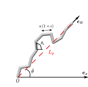
Refer to caption
Figure 2.4: Parameters of the numerical experiment. The angle θ¯¯𝜃\bar{\theta} is the average angle that the chain does with the horizontal axis (see eq.(2.57)) and 𝒆Rsubscript𝒆𝑅\bm{e}_{R} is the end-to-end direction. The projected length, indicated in red and denoted Lpsubscript𝐿𝑝L_{p}, is the length of the chain projected on 𝒆Rsubscript𝒆𝑅\bm{e}_{R}. Note that we impose the last segment to be parallel to 𝒆Rsubscript𝒆𝑅\bm{e}_{R}.

Each configuration ΩisubscriptΩ𝑖\Omega_{i} of the chain was described by the set {θ1,,θN1,ϵ}subscript𝜃1subscript𝜃𝑁1italic-ϵ\{\theta_{1},...,\theta_{N-1},\epsilon\}, where θisubscript𝜃𝑖\theta_{i} stands for the angle that the segment i𝑖i makes with the horizontal axis (see Fig. 2.4). The last segment was imposed always parallel to the vector 𝑹𝑹\bm{R}, defined by

𝑹=LNi=1i=N1𝒖i,𝑹𝐿𝑁superscriptsubscript𝑖1𝑖𝑁1subscript𝒖𝑖\bm{R}=\frac{L}{N}\sum_{i=1}^{i=N-1}\bm{u}_{i}\,, (2.56)

where 𝒖isubscript𝒖𝑖\bm{u}_{i} is the unitary vector in the direction of the i𝑖i-th segment so that τ1D=Σ1Dsubscript𝜏1Ddelimited-⟨⟩superscriptsubscriptΣparallel-to1D\tau_{\mathrm{1D}}=\langle\Sigma_{\parallel}^{\mathrm{1D}}\rangle can be easily checked through eq.(2.55). Associated to the vector 𝑹𝑹\bm{R}, we define the average direction 𝒆R𝑹/R𝒆subscript𝒆𝑅𝑹𝑅subscript𝒆parallel-to\bm{e}_{R}\equiv\bm{R}/R\equiv\bm{e}_{\parallel}, where R|𝑹|𝑅𝑹R\equiv|\bm{R}|. Thus we impose 𝒖N=𝒆Rsubscript𝒖𝑁subscript𝒆𝑅\bm{u}_{N}=\bm{e}_{R} and

θN=θ¯=1Ni=1i=Nθi.subscript𝜃𝑁¯𝜃1𝑁superscriptsubscript𝑖1𝑖𝑁subscript𝜃𝑖\theta_{N}=\bar{\theta}=\frac{1}{N}\sum_{i=1}^{i=N}\theta_{i}\,. (2.57)

The projected end-to-end length is given by Lp|𝑹|(L/N)i=1Ncos(θiθ¯)subscript𝐿𝑝𝑹𝐿𝑁superscriptsubscript𝑖1𝑁subscript𝜃𝑖¯𝜃L_{p}\equiv|\bm{R}|\equiv(L/N)\sum_{i=1}^{N}\cos(\theta_{i}-\bar{\theta}) (see Fig. 2.4).

During the simulation, we considered two kinds of moves:

  1. 1.

    Move A𝐴A: changing one segments angle θisubscript𝜃𝑖\theta_{i}, which corresponds to the effects of thermal fluctuations on the chain’s shape (see Fig. 2.5(a)). In this case, the direction 𝒆Rsubscript𝒆𝑅\bm{e}_{R} is changed and consequently, the last segment must have its direction corrected;

  2. 2.

    Move E𝐸E: changing the extension of segments through ϵitalic-ϵ\epsilon, which represents the exchange of lipids with the reservoir (see Fig. 2.5(b)).

Refer to caption
(a) Move A𝐴A: changing the angle of one segment with respect to the horizontal. The last segment must be adjusted so that its direction is parallel to the vector 𝒆Rsubscript𝒆𝑅\bm{e}_{R}.
Refer to caption
(b) Move E𝐸E: changing the extension ϵitalic-ϵ\epsilon of segments.
Figure 2.5: Two kinds of movements considered for the chain.

In addition, an external force 𝒇=τ𝒆R𝒇𝜏subscript𝒆𝑅\bm{f}=\tau\cdot\bm{e}_{R} always parallel to the last segment is exerted over the chain. The chain’s free-energy is given by a bending contribution, a contribution coming from the Lagrange multiplier σ𝜎\sigma plus a contribution from the external force

discret=σL+i=1N112κa(1+ϵ)Ci2τLp,subscriptdiscret𝜎𝐿superscriptsubscript𝑖1𝑁112𝜅𝑎1italic-ϵsuperscriptsubscript𝐶𝑖2𝜏subscript𝐿𝑝\mathcal{H}_{\mathrm{discret}}=\sigma L+\sum_{i=1}^{N-1}\frac{1}{2}\,\kappa\,a\,(1+\epsilon)\,C_{i}^{2}-\tau\,L_{p}\,, (2.58)

where

Ci=θi+1θia(1+ϵ)subscript𝐶𝑖subscript𝜃𝑖1subscript𝜃𝑖𝑎1italic-ϵC_{i}=\frac{\theta_{i+1}-\theta_{i}}{a\,(1+\epsilon)}\, (2.59)

is an approximation of the curvature between two successive segments. Note that the problem is invariant under rotation around the origin O𝑂O, so that at any moment we can describe the configuration on Monge’s gauge.

The imposed parameters of the simulation were N𝑁N, τ𝜏\tau in units of βa𝛽𝑎\beta\,a and κ𝜅\kappa in units of β𝛽\beta. For each τ𝜏\tau, σ𝜎\sigma was adjusted in order to fix ϵ=0delimited-⟨⟩italic-ϵ0\langle\epsilon\rangle=0, as discussed above. We detail how it was done in the following.

In the end of section 2.3.1, we have argued that in general, one should expect rτσ𝑟𝜏𝜎r\neq\tau\neq\sigma, where r𝑟r is the coefficient in q2superscript𝑞2q^{2} of the spectrum fluctuation

|hn|2=kBTrq2+κq4.delimited-⟨⟩superscriptsubscript𝑛2subscript𝑘B𝑇𝑟superscript𝑞2𝜅superscript𝑞4\langle|h_{n}|^{2}\rangle=\frac{k_{\mathrm{B}}T}{rq^{2}+\kappa q^{4}}\,. (2.60)

In order to measure |hn|2delimited-⟨⟩superscriptsubscript𝑛2\langle|h_{n}|^{2}\rangle (and thus r𝑟r), we have first performed a rotation so that we were in the same situation as in section 2.3.1. We defined Θ(x)=θiθ¯Θ𝑥subscript𝜃𝑖¯𝜃\Uptheta(x)=\theta_{i}-\bar{\theta}, where x𝑥x is the ordinate in the axis 𝒆xsubscript𝒆𝑥\bm{e}_{x}. The function Θ(x)Θ𝑥\Uptheta(x) is a series of steps of length cos(θiθ¯)subscript𝜃𝑖¯𝜃\cos(\theta_{i}-\bar{\theta}), as shown in Fig. 2.6. Note that this function is well-defined only when there are no overhangs (|θiθ¯|<π/2subscript𝜃𝑖¯𝜃𝜋2|\theta_{i}-\bar{\theta}|<\pi/2 for all segments), unlike the configuration seen on Fig. 2.4.
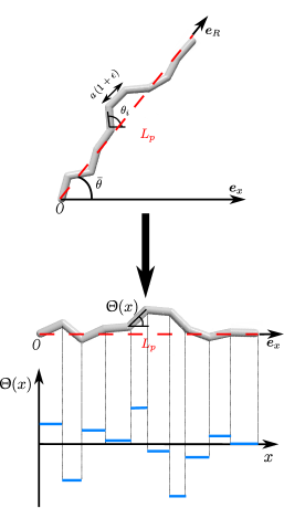
Refer to caption
Figure 2.6: Construction of function Θ(x)Θ𝑥\Uptheta(x). First, the initial configuration is rotated of θ¯¯𝜃-\,\bar{\theta}. The tension r𝑟r was deduced from the average of the Fourier transform of this curve over a large sample of configurations.

With the Fourier transform

Θn=0LpΘ(x)ei2πnxLp𝑑x,subscriptΘ𝑛superscriptsubscript0subscript𝐿𝑝Θ𝑥superscript𝑒𝑖2𝜋𝑛𝑥subscript𝐿𝑝differential-d𝑥\Uptheta_{n}=\int_{0}^{L_{p}}\Uptheta(x)\,e^{-i\,\frac{2\pi nx}{L_{p}}}\,dx\,, (2.61)

we expect

|Θn|21=β[r+κq2+𝒪(q4)],superscriptdelimited-⟨⟩superscriptsubscriptΘ𝑛21𝛽delimited-[]𝑟𝜅superscript𝑞2𝒪superscript𝑞4\langle|\Uptheta_{n}|^{2}\rangle^{-1}=\beta\left[r+\kappa q^{2}+\mathcal{O}(q^{4})\right]\,, (2.62)

with q=2πn/Lp𝑞2𝜋𝑛delimited-⟨⟩subscript𝐿𝑝q=2\pi n/\langle L_{p}\rangle. The strategy to obtain r𝑟r was to average |Θn|2superscriptsubscriptΘ𝑛2|\Uptheta_{n}|^{2} over a large set of configurations and fit the data with eq.(2.62). Fig. 2.7 shows a representative fit.
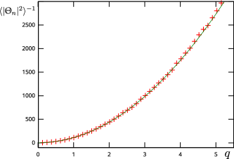
Refer to caption
Figure 2.7: Example the fit (solid line) of |Θn|21superscriptdelimited-⟨⟩superscriptsubscriptΘ𝑛21\langle|\Uptheta_{n}|^{2}\rangle^{-1} (crosses) with eq.(2.62) for N=50𝑁50N=50, κβ=125𝜅𝛽125\kappa\beta=125 and τβa=2𝜏𝛽𝑎2\tau\beta a=2 and σβa=2.45535𝜎𝛽𝑎2.45535\sigma\beta a=2.45535. The fit yields rβa=2.83±0.03𝑟𝛽𝑎plus-or-minus2.830.03r\beta a=2.83\pm 0.03 and κβ=109.28±0.09𝜅𝛽plus-or-minus109.280.09\kappa\beta=109.28\pm 0.09. Fit with χred2=0.82subscriptsuperscript𝜒2red0.82\chi^{2}_{\mathrm{red}}=0.82, indicating a good fit.

A sum-up of the variables can be seen in table 2.1.

Tension Status How
τ𝜏\tau imposed
σ𝜎\sigma adjusted L=Nadelimited-⟨⟩𝐿𝑁𝑎\langle L\rangle=N\,a
r𝑟r measured |Θn|2delimited-⟨⟩superscriptsubscriptΘ𝑛2\langle|\Uptheta_{n}|^{2}\rangle
Table 2.1: Sum-up of how we have dealt with tensions in the numerical experiment.
Numerical dynamics

We used a Monte Carlo method to generate a sufficiently large sample of chain’s configuration so that we could evaluate averages with a good precision [106]. The configurations were generated through a Markov chain algorithm: from a certain ΩisubscriptΩ𝑖\Omega_{i}, a random move of kind A𝐴A or E𝐸E was proposed, generating a new state Ωi+1subscriptΩ𝑖1\Omega_{i+1}. In order to respect the detailed balance, the configuration Ωi+1subscriptΩ𝑖1\Omega_{i+1} was accepted with the probability P(ΩiΩi+1)𝑃subscriptΩ𝑖subscriptΩ𝑖1P(\Omega_{i}\rightarrow\Omega_{i+1}) given by the Metropolis algorithm

P(ΩiΩi+1)=min[1,p(Ωi+1)p(Ωi)].𝑃subscriptΩ𝑖subscriptΩ𝑖11𝑝subscriptΩ𝑖1𝑝subscriptΩ𝑖P(\Omega_{i}\rightarrow\Omega_{i+1})=\min\left[1,\frac{p(\Omega_{i+1})}{p(\Omega_{i})}\right]\,. (2.63)

In the case of thermodynamic equilibrium, the probability of each configuration is given by the Boltzmann distribution

p(Ωi)=eβdiscret(Ωi)𝒵,𝑝subscriptΩ𝑖superscript𝑒𝛽subscriptdiscretsubscriptΩ𝑖𝒵p(\Omega_{i})=\frac{e^{-\beta\,\mathcal{H}_{\mathrm{discret}}(\Omega_{i})}}{\mathcal{Z}}\,, (2.64)

where 𝒵𝒵\mathcal{Z} is the partition function. The probability of transition is then simply given by

P(ΩiΩi+1)=min[1,eβΔ],𝑃subscriptΩ𝑖subscriptΩ𝑖11superscript𝑒𝛽ΔP(\Omega_{i}\rightarrow\Omega_{i+1})=\min\left[1,e^{-\beta\,\Delta\mathcal{H}}\right]\,, (2.65)

where Δ=discret(Ωi+1)discret(Ωi)ΔsubscriptdiscretsubscriptΩ𝑖1subscriptdiscretsubscriptΩ𝑖\Delta\mathcal{H}=\mathcal{H}_{\mathrm{discret}}(\Omega_{i+1})-\mathcal{H}_{\mathrm{discret}}(\Omega_{i}). In our case, we have

  1. 1.

    move A𝐴A: an angle θisubscript𝜃𝑖\theta_{i} of the set {θ1,,θN1}subscript𝜃1subscript𝜃𝑁1\{\theta_{1},...,\theta_{N-1}\} is randomly chosen. We propose a new angle θi=θi+Δθsuperscriptsubscript𝜃𝑖subscript𝜃𝑖Δ𝜃\theta_{i}^{\prime}=\theta_{i}+\Delta\theta, where Δθ=δθ×rand(1,1)Δ𝜃subscript𝛿𝜃rand11\Delta\theta=\delta_{\theta}\times\,\mathrm{rand}(-1,1), with rand(a,b)rand𝑎𝑏\mathrm{rand}(a,b) a random number with uniform distribution of probability between a𝑎a and b𝑏b. The new θ¯superscript¯𝜃\bar{\theta}^{\prime} is evaluated and consequently θN=θ¯superscriptsubscript𝜃𝑁superscript¯𝜃\theta_{N}^{\prime}=\bar{\theta}^{\prime}. The variation of free-energy is thus

    ΔAΔsubscript𝐴\displaystyle\Delta\mathcal{H}_{A} =\displaystyle= κ2a(1+ϵ)[(θi+1θi)2(θi+1θi)2+(θiθi1)2\displaystyle\frac{\kappa}{2\,a(1+\epsilon)}\left[\left(\theta_{i+1}-\theta_{i}^{\prime}\right)^{2}-\left(\theta_{i+1}-\theta_{i}\right)^{2}+\left(\theta_{i}^{\prime}-\theta_{i-1}\right)^{2}\right. (2.66)
    \displaystyle- (θiθi1)2+(θNθN1)2(θNθN1)2]\displaystyle\left.\left(\theta_{i}-\theta_{i-1}\right)^{2}+\left(\theta_{N}^{\prime}-\theta_{N-1}\right)^{2}-\left(\theta_{N}-\theta_{N-1}\right)^{2}\right]
    \displaystyle- τLN[j=0j=Ncos(θjθ¯)j=0j=Ncos(θjθ¯)].𝜏𝐿𝑁delimited-[]superscriptsubscript𝑗0𝑗𝑁subscript𝜃𝑗superscript¯𝜃superscriptsubscript𝑗0𝑗𝑁subscript𝜃𝑗¯𝜃\displaystyle\tau\,\frac{L}{N}\left[\sum_{j=0}^{j=N}\cos\left(\theta_{j}-\bar{\theta}^{\prime}\right)-\sum_{j=0}^{j=N}\cos\left(\theta_{j}-\bar{\theta}\right)\right]\,.

    If i=0𝑖0i=0, the third and the fourth terms should not be taken into account. The value of δθsubscript𝛿𝜃\delta_{\theta} is chosen in order to have 50%absentpercent50\approx 50\% of acceptance of this kind of move.

  2. 2.

    move E𝐸E: a new extension ϵ=ϵ+Δϵsuperscriptitalic-ϵitalic-ϵΔitalic-ϵ\epsilon^{\prime}=\epsilon+\Delta\epsilon, with Δϵ=δϵ×rand(1,1)Δitalic-ϵsubscript𝛿italic-ϵrand11\Delta\epsilon=\delta_{\epsilon}\times\,\mathrm{rand}(-1,1) is proposed. The free-energy variation reads

    ΔEΔsubscript𝐸\displaystyle\Delta\mathcal{H}_{E} =\displaystyle= σaΔϵτaΔϵj=0j=Ncos(θjθ¯)𝜎𝑎Δitalic-ϵ𝜏𝑎Δitalic-ϵsuperscriptsubscript𝑗0𝑗𝑁subscript𝜃𝑗¯𝜃\displaystyle\sigma\,a\,\Delta\epsilon-\tau\,a\,\Delta\epsilon\sum_{j=0}^{j=N}\cos\left(\theta_{j}-\bar{\theta}\right) (2.67)
    +\displaystyle+ κΔϵ2a(1+ϵ)(1+ϵ)j=0j=N1(θj+1θj)2.𝜅Δitalic-ϵ2𝑎1italic-ϵ1superscriptitalic-ϵsuperscriptsubscript𝑗0𝑗𝑁1superscriptsubscript𝜃𝑗1subscript𝜃𝑗2\displaystyle\frac{\kappa\,\Delta\epsilon}{2\,a(1+\epsilon)(1+\epsilon^{\prime})}\sum_{j=0}^{j=N-1}\left(\theta_{j+1}-\theta_{j}\right)^{2}\,.

    Again, δϵsubscript𝛿italic-ϵ\delta_{\epsilon} was chosen in order to have 50%absentpercent50\approx 50\% of acceptance for moves of kind E𝐸E.

To each move of kind E𝐸E, N1𝑁1N-1 moves of kind A𝐴A were tried in order to assure that in average every degree of freedom is equally modified. In the following, we will call this sequence a Monte Carlo step.

Equilibration criterion

In order to obtain meaningful averages, we had to be sure that our numerical experiment reached equilibrium. Usually, it is enough to examine the number of Monte Carlo steps needed to decorrelate the longest modes on the Fourier space, which are the slowest to relax, and then choose a number of steps much larger for the simulation[106]. As our system is really simple (in the sense that the energy do not have several local minima) and that we have not chosen too long chains, we have chosen two criterion that together are stronger than the relaxation of the longest modes. First, for the equilibration of angles, we have required the average of 𝑹𝑹\bm{R}, given in eq.(2.56), to be 0similar-toabsent0\sim 0. One could imagine the case of a rotating fixed configuration, which would also yield 𝑹0similar-todelimited-⟨⟩𝑹0\langle\bm{R}\rangle\sim 0. To exclude this improbable situation, we have visually checked a set of configurations. Secondly, to study the equilibration of the extension ϵitalic-ϵ\epsilon, we have examined the evolution of ϵdelimited-⟨⟩italic-ϵ\langle\epsilon\rangle over time: when it reached a plateau, we considered the system at equilibrium.

In our experiments, we have taken N=50𝑁50N=50 and a larger βκ=125𝛽𝜅125\beta\kappa=125 to assure that the chain departs weakly from a straight line. For typical values ranging from τ=0.2βa𝜏0.2𝛽𝑎\tau=-0.2\,\beta a up to τ=5βa𝜏5𝛽𝑎\tau=5\,\beta a, the equilibration was attained after 5×1055superscript1055\times 10^{5} steps. Currently, we have made 8×1068superscript1068\times 10^{6} steps to be sure that the sampled configurations had an equilibrium distribution. At the end of each step, we have calculated Θ(x)Θ𝑥\Uptheta(x) (when there were no overhangs).

Adjusting σ𝜎\sigma

As we applied τ𝜏\tau to the membrane, we had to adjust σ𝜎\sigma in order to have ϵ0similar-todelimited-⟨⟩italic-ϵ0\langle\epsilon\rangle\sim 0. To estimate also the uncertainty of σ𝜎\sigma, for each pair κ,τ𝜅𝜏\kappa,\tau we determined σminsubscript𝜎min\sigma_{\mathrm{min}} corresponding to ϵmax=ϵ=103subscriptitalic-ϵmaxdelimited-⟨⟩italic-ϵsuperscript103\epsilon_{\mathrm{max}}=\langle\epsilon\rangle=10^{-3} and σmaxsubscript𝜎max\sigma_{\mathrm{max}} corresponding to ϵmin=ϵ=103subscriptitalic-ϵmindelimited-⟨⟩italic-ϵsuperscript103\epsilon_{\mathrm{min}}=\langle\epsilon\rangle=-10^{-3}. To do so, we inspired ourselves on eq.(2.54)

(στ1D)βa=32π0.5,𝜎subscript𝜏1D𝛽𝑎32𝜋similar-to-or-equals0.5\left(\sigma-\tau_{\mathrm{1D}}\right)\beta a=\frac{3}{2\pi}\simeq 0.5\,, (2.68)

and started with two guesses (σminτ)βa=0.35subscript𝜎min𝜏𝛽𝑎0.35(\sigma_{\mathrm{min}}-\tau)\beta a=0.35 and (σmaxτ)βa=0.55subscript𝜎max𝜏𝛽𝑎0.55(\sigma_{\mathrm{max}}-\tau)\beta a=0.55. The approach of the boundaries ϵmaxsubscriptitalic-ϵmax\epsilon_{\mathrm{max}} and ϵminsubscriptitalic-ϵmin\epsilon_{\mathrm{min}} was made through a false-point algorithm in 202020 iterations at maximum [107]. The stop criterion for σminsubscript𝜎min\sigma_{\mathrm{min}} was |ϵϵmin|<3×10⁴delimited-⟨⟩italic-ϵsubscriptitalic-ϵmin3superscript104|\langle\epsilon\rangle-\epsilon_{\mathrm{min}}|<3\times 10^{-4} and equivalently |ϵϵmax|<3×10⁴delimited-⟨⟩italic-ϵsubscriptitalic-ϵmax3superscript104|\langle\epsilon\rangle-\epsilon_{\mathrm{max}}|<3\times 10^{-4} for σmaxsubscript𝜎max\sigma_{\mathrm{max}}. A fluxogram of the adjustment procedure is presented in Fig. 2.8. For the typical values presented in the last section, the difference σmaxσminsubscript𝜎maxsubscript𝜎min\sigma_{\mathrm{max}}-\sigma_{\mathrm{min}} was systematically of 0.001βaabsent0.001𝛽𝑎\approx 0.001\,\beta a.

Refer to caption
Figure 2.8: Fluxogram of the adjustment procedure. The processes taking place in the main function roda.c are inside violet boxes (solid lines). Each blue box (dashed lines) indicates a run of Monte Carlo of 8×1068superscript1068\times 10^{6} steps. The brown box (dotted lines) indicates that the false-point algorithm was used to suggest a new σ𝜎\sigma. It is called at most 202020 times for each boundary (usually, less than 555 times were enough).
Buckling transition

In order to verify the correctness of our simulation, we have also applied negative tensions to the filament. Indeed, for compressive tensions bigger than a certain limit, we expect our filament to fluctuate around a curved line, instead than around a straight line, as shown in Fig. 2.9. This transition is known as the buckling transition.

This transition is also characterized by an increase and a discontinuity on the length excess, the equivalent of α𝛼\alpha, defined as

α1D=LLpLp,subscript𝛼1D𝐿delimited-⟨⟩subscript𝐿𝑝delimited-⟨⟩subscript𝐿𝑝\alpha_{\mathrm{1D}}=\frac{L-\langle L_{p}\rangle}{\langle L_{p}\rangle}\,, (2.69)

as the compressive tension increases. In Fig. 2.10 we can see that we have effectively a relatively abrupt increase of α1Dsubscript𝛼1D\alpha_{\mathrm{1D}} as the tension approaches τ=0.3βa𝜏0.3𝛽𝑎\tau=-0.3\beta a. We have thus some evidence of a buckling transition for negative tensions. We have not however made a systematic study of the transition, since it was not the aim our numerical experiment. Moreover, we have found some technical problems for τ0.3βa𝜏0.3𝛽𝑎\tau\leq-0.3\beta a, since the projected length was highly fluctuating due to the alternating presence of buckled and straight configurations near the transition. The averages varied a lot and thus, with the parameters presented in the last section, the false-point method failed to converge in 202020 iterations. Therefore, we have just considered τ0.2βa𝜏0.2𝛽𝑎\tau\geqslant-0.2\beta a, situation in which we are sure that we had small fluctuations around a straight line.
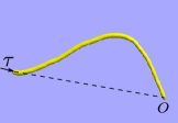
Refer to caption
(a) Buckled configuration for τ=0.3βa𝜏0.3𝛽𝑎\tau=-0.3\,\beta a.
Refer to caption
(b) Non-buckled configuration for τ=0.5βa𝜏0.5𝛽𝑎\tau=0.5\,\beta a.
Figure 2.9: Buckling transition.
Refer to caption
Figure 2.10: Percent length excess as a function of τ𝜏\tau. The shaded region on the left represents the approach of the buckling transition.
2.3.3 Results

Once σminsubscript𝜎min\sigma_{\mathrm{min}} and σmaxsubscript𝜎max\sigma_{\mathrm{max}} were found, we have performed the numerical experiment three times with each value. We have taken the average of these three runs for the spectrum and for the average curvature of the last segment. For each averaged spectrum, we have made a fit using gnuplot to obtain r𝑟r (see Fig. 2.7 for an example). We obtained κβ110𝜅𝛽110\kappa\beta\approx 110 in all fits, which we remind is a bit different from the microscopical κβ=125𝜅𝛽125\kappa\beta=125. This result is coherent with what one should expect given eq.(1.30), which takes into account corrections due to the renormalization. The final results are summed up in table 2.2. In this table, σ𝜎\sigma and r𝑟r are the averages of σmaxsubscript𝜎max\sigma_{\mathrm{max}} and σminsubscript𝜎min\sigma_{\mathrm{min}} and the corresponding r𝑟r. From table 2.2, it is evident that τσ𝜏𝜎\tau\neq\sigma (see also Fig. 2.11). In the same graphic, we have also plotted σt=σκCLp2/2delimited-⟨⟩subscript𝜎𝑡𝜎𝜅delimited-⟨⟩superscriptsubscript𝐶subscript𝐿𝑝22\langle\sigma_{t}\rangle=\sigma-\kappa\langle C_{L_{p}}^{2}\rangle/2. As predicted, we have indeed σt=τdelimited-⟨⟩subscript𝜎𝑡𝜏\langle\sigma_{t}\rangle=\tau.

Refer to caption
Figure 2.11: Tensions τ𝜏\tau (diamonds) and σ𝜎\sigma (circles on top) as a function of the shortening of the projected length. Note that as predicted, the average of the tangential stress tensor at the extremity σtdelimited-⟨⟩subscript𝜎𝑡\langle\sigma_{t}\rangle (circles superposed with the diamonds) coincides with τ𝜏\tau. The dashed lines are just guides to the eye.
τ𝜏\tau σ𝜎\sigma r𝑟r κ/2CLp2𝜅2delimited-⟨⟩superscriptsubscript𝐶subscript𝐿𝑝2\kappa/2\langle C_{L_{p}}^{2}\rangle Lpdelimited-⟨⟩subscript𝐿𝑝\langle L_{p}\rangle
-0.2 0.31 0.01 0.48 48.81
-0.1 0.40 0.17 0.47 48.91
0 0.50 0.32 0.47 48.99
0.5 0.98 0.97 0.46 49.20
1 1.47 1.63 0.45 49.32
1.5 1.96 2.24 0.44 49.38
2 2.46 2.81 0.43 49.43
2.5 2.95 3.45 0.42 49.48
3 3.44 4.11 0.42 49.51
3.5 3.94 4.53 0.41 49.55
4 4.43 5.19 0.41 49.56
4.5 4.93 5.71 0.41 49.59
5 5.42 6.16 0.4 49.59
Table 2.2: Sum-up of the results obtained from our numerical experiment for N=50𝑁50N=50 and βκ=125𝛽𝜅125\beta\kappa=125. The values of the four first columns are in units of βa𝛽𝑎\beta a, while the last column is in units of a𝑎a. The errors on the second and third column are of 0.001absent0.001\approx 0.001 and 0.02absent0.02\approx 0.02 respectively. The fourth column is the average of the curvature energy of the last segment.

Quantitatively, the fit with the theoretical equation for the difference στ𝜎𝜏\sigma-\tau given in eq.(2.53) can be seen in Fig. 2.12 (solid line). The agreement is excellent for Λ=1.1a1Λ1.1superscript𝑎1\Lambda=1.1\,a^{-1} (one parameter fit), which is a very reasonable value for the cut-off. In this graphics, we have also plotted the percent difference between σ𝜎\sigma and r𝑟r. The behavior is non-trivial: the sign of σr𝜎𝑟\sigma-r changes at low tensions and we have σr𝜎𝑟\sigma\neq r even at high tensions.

Refer to caption
Figure 2.12: Lower data: comparison between τ𝜏\tau and σ𝜎\sigma (error bars given by the symbol size); the solid line is a fit using eq.(2.53). Upper data: comparison between r𝑟r and σ𝜎\sigma; the dashed is only a guide for the eye.

To conclude, with this simple numerical experiment, we could accede to the tension σ𝜎\sigma needed to fix the length of the filament, which one cannot usually measure in true experiments, simultaneously to the tension τ𝜏\tau and r𝑟r. Our data corroborates the prediction that τσ𝜏𝜎\tau\neq\sigma and verify eq.(2.55). In addition, the difference between τ𝜏\tau and σ𝜎\sigma was well fitted by eq.(2.3.1), giving some support to our theory. Regarding r𝑟r, as discussed in section 2.2.3, we expected in general τσr𝜏𝜎𝑟\tau\neq\sigma\neq r, which our data seems to confirm. The way in which r𝑟r depends on σ𝜎\sigma seems to be non-trivial (see Fig. 2.12) and further studies have to be done in order to understand it.

2.4 Some experimental implications

In this section, we discuss the implications of eq.(2.10) to micropipette experiments. Indeed, in these experiments, it is usually assumed that στ𝜎𝜏\sigma\approx\tau, which, as we have seen, is not justified in the limit of low tensions. We will assume that we are dealing with very large GUV and that the difference of pressure between the inside and the outside of the vesicle is very small, so that the membrane is locally equivalent to a flat membrane. A more detailed derivation for quasi-spherical vesicles of any size taking into account the pressure difference will be done in chapter 4.

In the limit of small fluctuations, the excess area is given by

α=AApAp𝛼delimited-⟨⟩𝐴subscript𝐴𝑝subscript𝐴𝑝\displaystyle\alpha=\frac{\langle A\rangle-A_{p}}{A_{p}} similar-to-or-equals\displaystyle\simeq 12(h)2,12delimited-⟨⟩superscript2\displaystyle\frac{1}{2}\,\langle(\nabla h)^{2}\rangle\,, (2.70)
similar-to-or-equals\displaystyle\simeq kBT2Ap𝒒1σ+κq2,subscript𝑘B𝑇2subscript𝐴𝑝subscript𝒒1𝜎𝜅superscript𝑞2\displaystyle\frac{k_{\mathrm{B}}T}{2A_{p}}\sum_{\bm{q}}\frac{1}{\sigma+\kappa q^{2}}\,,

where we have used the correlation function given in eq.(2.7). In the thermodynamic limit, we have

α𝛼\displaystyle\alpha similar-to-or-equals\displaystyle\simeq kBT8πκln(σ+σrσ+κ(2π)2Ap),subscript𝑘B𝑇8𝜋𝜅𝜎subscript𝜎𝑟𝜎𝜅superscript2𝜋2subscript𝐴𝑝\displaystyle\frac{k_{\mathrm{B}}T}{8\pi\kappa}\ln\left(\frac{\sigma+\sigma_{r}}{\sigma+\kappa\frac{(2\pi)^{2}}{A_{p}}}\right)\,, (2.71)
similar-to-or-equals\displaystyle\simeq kBT8πκln(σrσ),subscript𝑘B𝑇8𝜋𝜅subscript𝜎𝑟𝜎\displaystyle\frac{k_{\mathrm{B}}T}{8\pi\kappa}\ln\left(\frac{\sigma_{r}}{\sigma}\right)\,, (2.72)

where the last approximation is valid in the limit κ/Apσ102σrmuch-less-than𝜅subscript𝐴𝑝𝜎less-than-or-similar-tosuperscript102subscript𝜎𝑟\kappa/A_{p}\ll\sigma\lesssim 10^{-2}\,\sigma_{r}. Using the fact that in this limit στ+σ0similar-to-or-equals𝜎𝜏subscript𝜎0\sigma\simeq\tau+\sigma_{0}, we have finally

αkBT8πκln(σrσ0+τ).similar-to-or-equals𝛼subscript𝑘B𝑇8𝜋𝜅subscript𝜎𝑟subscript𝜎0𝜏\alpha\simeq\frac{k_{\mathrm{B}}T}{8\pi\kappa}\ln\left(\frac{\sigma_{r}}{\sigma_{0}+\tau}\right)\,. (2.73)

In micropipette experiments, one measures the percent difference of projected area between the initial configuration Apisuperscriptsubscript𝐴𝑝𝑖A_{p}^{i} and the final configuration Apfsuperscriptsubscript𝐴𝑝𝑓A_{p}^{f}:

ApfApiApisuperscriptsubscript𝐴𝑝𝑓superscriptsubscript𝐴𝑝𝑖superscriptsubscript𝐴𝑝𝑖\displaystyle\frac{A_{p}^{f}-A_{p}^{i}}{A_{p}^{i}} =\displaystyle= (AApiApi)(AApfApi),delimited-⟨⟩𝐴superscriptsubscript𝐴𝑝𝑖superscriptsubscript𝐴𝑝𝑖delimited-⟨⟩𝐴superscriptsubscript𝐴𝑝𝑓superscriptsubscript𝐴𝑝𝑖\displaystyle\left(\frac{\langle A\rangle-A_{p}^{i}}{A_{p}^{i}}\right)-\left(\frac{\langle A\rangle-A_{p}^{f}}{A_{p}^{i}}\right)\,, (2.74)
similar-to-or-equals\displaystyle\simeq αiαfsubscript𝛼𝑖subscript𝛼𝑓\displaystyle\alpha_{i}-\alpha_{f}\,
similar-to-or-equals\displaystyle\simeq kBT8πκln(σfσi),subscript𝑘B𝑇8𝜋𝜅subscript𝜎𝑓subscript𝜎𝑖\displaystyle\frac{k_{\mathrm{B}}T}{8\pi\kappa}\ln\left(\frac{\sigma_{f}}{\sigma_{i}}\right)\,,
similar-to-or-equals\displaystyle\simeq kBT8πκln(σ0+τfσ0+τi).subscript𝑘B𝑇8𝜋𝜅subscript𝜎0subscript𝜏𝑓subscript𝜎0subscript𝜏𝑖\displaystyle\frac{k_{\mathrm{B}}T}{8\pi\kappa}\ln\left(\frac{\sigma_{0}+\tau_{f}}{\sigma_{0}+\tau_{i}}\right)\,. (2.75)

Eq.(2.74) corresponds to the result presented in section 1.4.1 and usually used to deduce κ𝜅\kappa by considering τσ𝜏𝜎\tau\approx\sigma. In eq.(2.75), we see the explicit relation as a function of τ𝜏\tau.

In Fig. 2.13, we imagine a typical micropipette experiment with a vesicle initially under very small tension τi=108N/msuperscript𝜏𝑖superscript108Nm\tau^{i}=10^{-8}\,\mathrm{N/m} and κ=25kBT𝜅25subscript𝑘B𝑇\kappa=25\,k_{\mathrm{B}}T. We increase the tension up to 104N/msuperscript104Nm10^{-4}\,\mathrm{N/m} by aspiring the vesicle. The curves in Fig. 2.13 represent the expected relation between the logarithm of τf/τisuperscript𝜏𝑓superscript𝜏𝑖\tau^{f}/\tau^{i} and the percent of increase in the projected area for τ=σ𝜏𝜎\tau=\sigma and for τ=σσ0𝜏𝜎subscript𝜎0\tau=\sigma-\sigma_{0}.

First of all, note that the percent increase of the projected area is very small (less than 0.5%percent0.50.5\%), which corresponds to the validity range of our results (no stretching). For τ>σ0𝜏subscript𝜎0\tau>\sigma_{0}, we have a linear dependence of the logarithm of τ𝜏\tau on the percent projected area with roughly the same slope whether one takes into account the difference between τ𝜏\tau and σ𝜎\sigma (eq.(2.75)) or not (eq.(2.74)). Thus, it is justified to deduce κ𝜅\kappa by fitting a straight line to data on this region, as it is usually experimentally done (see section 4, Fig. 1.28.(a)). We predict however a different behavior for small tensions (τ<σ0𝜏subscript𝜎0\tau<\sigma_{0}): as we can see in Fig. 2.13, in the shaded area, we do not have a linear relation between the logarithm of τ𝜏\tau and the area excess. Sadly, we cannot identify this behavior in the data of Fig. 1.28, but our prediction can be tested by further experiments using vesicles under small tension.
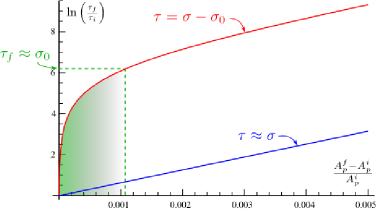
Refer to caption
Figure 2.13: Theoretical relation linking the tension to the difference of the projected area: in red (upper curve), we see the curve where the distinction between τ𝜏\tau and σ𝜎\sigma is taken in account (eq.(2.75)), while in blue (lower straight line) we see the usual law, supposing that τ=σ𝜏𝜎\tau=\sigma (eq.(2.74)). Numerical values: kBT=4×10²¹Jsubscript𝑘B𝑇4superscript1021Jk_{\mathrm{B}}T=4\times 10^{-21}\,\mathrm{J}, κ=1019J𝜅superscript1019J\kappa=10^{-19}\,\mathrm{J}, a=5nm𝑎5nma=5\,\mathrm{nm}. We considered a vesicle under initial tension τi=108N/msuperscript𝜏𝑖superscript108Nm\tau^{i}=10^{-8}\,\mathrm{N/m}. The tension is increased up to τ=104N/m𝜏superscript104Nm\tau=10^{-4}\,\mathrm{N/m}. Note that for τ<σ0𝜏subscript𝜎0\tau<\sigma_{0}, we have no more a linear behavior.
2.4.1 Natural excess area

Another related consequence concerns the natural excess area, i. e., the measure of the fluctuations of a membrane under no external force (τ=0𝜏0\tau=0). Using eq.(2.73), we have

αeqln(8πβκ)8πβκ,similar-to-or-equalssubscript𝛼eq8𝜋𝛽𝜅8𝜋𝛽𝜅\alpha_{\mathrm{eq}}\simeq\frac{\ln(8\pi\beta\kappa)}{8\pi\beta\kappa}\,, (2.76)

which yields αeq0.03,0.01,0.005similar-to-or-equalssubscript𝛼eq0.030.010.005\alpha_{\mathrm{eq}}\simeq 0.03,0.01,0.005 for βκ=5,25,50𝛽𝜅52550\beta\kappa=5,25,50, respectively.

Traditionally, however, one makes σ=0𝜎0\sigma=0 in eq.(2.70), which leads to

αeqtrad14πβκln(ΛAp2π).similar-to-or-equalssuperscriptsubscript𝛼eqtrad14𝜋𝛽𝜅Λsubscript𝐴𝑝2𝜋\alpha_{\mathrm{eq}}^{\mathrm{trad}}\simeq\frac{1}{4\pi\beta\kappa}\ln\left(\frac{\Lambda\sqrt{A_{p}}}{2\pi}\right)\,. (2.77)

The main difference between these equations is the dependence in terms of the projected area Apsubscript𝐴𝑝A_{p}, since for the last equation one expects an explicit logarithmic dependence. Eq.(2.76) presents also a hidden dependence on Apsubscript𝐴𝑝A_{p} through eq.(1.30) due to renormalization, although it should be a far weaker dependence. This result is well suited for numerical verifications.

2.5 First evidences that τσ𝜏𝜎\tau\neq\sigma

Here we present the first strong numerical and experimental evidences of the correctness of our results. In the first part, we present the results of recent numerical experiments far more complex than the one presented in section 2.3. In the second part, we discuss experiments on the adhesion of vesicles to solid substrate. We begin by mentioning a previous puzzling result by Rädler et al. [84], already introduced in section 1.4.3. We report the attempts to understand this result made by Seifert [108]. Finally, we describe a recent experiment that seems to corroborate our previsions [87].

2.5.1 Numerical experiments

In the same ref. [3], discussed in section 2.2, a 222-d numerical experiment was proposed to check the author’s predictions. The numerical system consisted on coarse-grained amphiphilic lipids represented by chains of beads (see Fig. 2.14). The black beads represent the hydrophobic tail, while the white one stands for the hydrophilic head. In addition, single beads stood for water molecules.
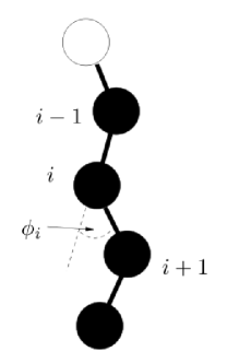
Refer to caption
Figure 2.14: Coarse-grained amphiphilic molecule used in the numerical experiment proposed in ref. [3]. The black beads represent the molecule’s hydrophobic tail, while the hydrophilic head is represented by the white bead.

The total energy was composed by four terms:

  1. 1.

    the hydrophobic interaction between the beads of the tail and water/hydrophilic head;

  2. 2.

    an attractive interaction between two molecules, given by a Lennard-Jones potential;

  3. 3.

    a harmonic potential between beads along a single molecule;

  4. 4.

    a three-body bending potential that models the effects of hydrocarbon chain stiffness.

Both molecules of lipids and water were free to move inside a fixed cuboidal box with periodic boundary conditions. At each realization of the simulation, the size of the box could be changed, implying a change in the membranes tension τ𝜏\tau. The dynamics alternated sequences of Monte Carlo steps with sequences of molecular dynamics steps.

In order to measure τ𝜏\tau, the forces exchanged through imaginary cuts perpendicular to the membrane plane were averaged for different box sizes. As in real experiments, the tension r𝑟r was measured through the fluctuation spectrum. Similarly with our simple 111-d simulation, the buckling transition was observed for high compressive tensions. For the non-buckled regime, the results for a simulation involving 115211521152 amphiphilic molecules and 720072007200 water molecules can be seen in Fig. 2.15. In agreement with the discussion of section 2.2, the author obtained indeed τr𝜏𝑟\tau\neq r. Moreover, negative tensions are observed for non-buckled membranes, as in our case.

In this work, the relation given in eq.(2.9) was obtained by differentiating the free-energy with respect to the projected area. Assuming that rσ𝑟𝜎r\approx\sigma, as usually done in laboratory experiments, the author fitted eq.(2.9) to τ𝜏\tau by adjusting one parameter related to the upper wave-length cutoff. As we an see in Fig. 2.16, the agreement is very good, supporting the predicted relation between τ𝜏\tau and σ𝜎\sigma given in eq.(2.9).

Refer to caption
Figure 2.15: Plot of r𝑟r (indicated by a circle) and τ𝜏\tau (black circle) as a function of the projected area per molecule apsubscript𝑎𝑝a_{p} obtained in ref. [3]. As apsubscript𝑎𝑝a_{p} increases, the fluctuations are flattened and the tension τ𝜏\tau increases. The tension is displayed in units of ϵ/2italic-ϵsuperscript2\epsilon/\ell^{2} and apsubscript𝑎𝑝a_{p} in units of 2superscript2\ell^{2}, with ϵ=1/3×1020Jitalic-ϵ13superscript1020J\epsilon=1/3\times 10^{-20}\,\mathrm{J} and =1/3nm13nm\ell=1/3\mathrm{nm}.
Refer to caption
Figure 2.16: The black squares indicate the directly measured tension τ𝜏\tau in ref. [3]. The circles represent the fitted values using eq.(2.9) and assuming rσ𝑟𝜎r\approx\sigma. The units are the same as in the last figure.

Very recently, a similar simulation was performed by Neder et al. [109]. They have also used coarse-grained amphiphilic molecules similar to the one shown in Fig. 2.14 and the energy contributions were roughly the same as in [3], added of a term τAp𝜏subscript𝐴𝑝-\tau\,A_{p}. Thus, the main difference in this simulation is the fact that τ𝜏\tau is imposed (and not measured) and the box size was free to change. In other words, the simulation was performed at τ𝜏\tau and Npsubscript𝑁𝑝N_{p}, the number of lipids, fixed. The advantage of this method is the possibility of controlling directly τ𝜏\tau, while in the method used in [3], the tension was imposed by the size of the box. The configurations were generated through a Monte Carlo algorithm, since only static measures were done. Different phases of the membrane were observed, depending on the temperature of the system. In particular, we can see some snapshots for the liquid phase in Fig. 2.17.

Refer to caption
Figure 2.17: Snapshots of bilayer configurations in the liquid phase [109]. The dark gray molecules point upward from tail to head while the light gray point downward. In the first snapshot at left, the membrane is tensionless. In the following two snapshots, the tension is increased (0.01J/m20.01Jsuperscriptm20.01\,\mathrm{J/m^{2}} and 0.02J/m20.02Jsuperscriptm20.02\,\mathrm{J/m^{2}}, respectively). Remark the interdigitations in the configuration of highest tension due to the stretching of the membrane.

As before, r𝑟r was measured through the fluctuation spectrum for the tensions above mentioned (results presented in table III𝐼𝐼𝐼III of [109]). For the tensionless state, they obtained r=(0.11±0.19)×104J/m2𝑟plus-or-minus0.110.19superscript104Jsuperscriptm2r=(0.11\pm 0.19)\times 10^{-4}\,\mathrm{J/m^{2}}. This result seems to agree with our prediction that r𝑟r should be bigger than τ𝜏\tau, even though one should be cautious given the large error-bars. For the systems under higher tension, however, the trend was inverted. This fact does not contradict our predictions, since stretching was not taken into account in our theory. Indeed, by measuring an overlap parameter, as well as the nematic order parameter for the liquid phase, the authors confirmed that stretching takes place for τ0.01J/m2greater-than-or-equivalent-to𝜏0.01Jsuperscriptm2\tau\gtrsim 0.01\,\mathrm{J/m^{2}}. Further simulations in the regime of low tension should be useful to compare with our predictions.

2.5.2 Adhesion experiments: a puzzling result

Here we will comment on some experiments involving the adhesion of vesicles to solid flat substrates, discussed in section 1.4.3. In 1995, Rädler et al. [84] studied the adhesion of GUVs to solid substrates. They constituted GUVs of stearoyl-oleoyl-phosphatidylcholine (SOPC) in a 100mM100mM100\,\,\mathrm{mM} sucrose solution, so that the vesicles were denser than the buffer solution and sank to the bottom of the chamber, where a glass cover slip coated with a thin film of MgF2𝑀𝑔superscript𝐹2MgF^{2} and bovine serum albumin had been deposed. The vesicle then floated above the glass slip with a height s(𝒓)𝑠𝒓s(\bm{r}), as shown in Fig. 1.33(b), in a weakly adhered state. Using reflection interference contrast microscopy (RICM) and phase contrast microscopy (see Fig. 2.18), the group could measure the radius of the vesicle Rvessubscript𝑅vesR_{\mathrm{ves}}, the radius of the contact region Rasubscript𝑅𝑎R_{a}, and reconstruct the height profile of the adhered patch.
Refer to caption
(a) High tension (the bar corresponds to 10μm10𝜇m10\,\mathrm{\mu m}).
Refer to caption
(b) Small tension
Figure 2.18: RICM micrographs of adhering vesicles under different tensions [84]. The height profile is obtained by measuring the intensity of light through a line that passes by the center of the contact region. The fringes at the edge of the round area indicate the end of the contact region.

Under the supposition that energy of the contact region was well described by eq.(1.38) and defining h(𝒓)=s(𝒓)s𝒓𝑠𝒓delimited-⟨⟩𝑠h(\bm{r})=s(\bm{r})-\langle s\rangle, they could infer:

  1. 1.

    the fluctuation spectrum |h(𝒒)|2delimited-⟨⟩superscript𝒒2\langle|h(\bm{q})|^{2}\rangle, which once fitted with eq.(1.39) allowed to obtain r𝑟r and V′′superscript𝑉′′V^{\prime\prime} (see Fig. 2.19). The bending rigidity for SOPC, obtained in previous experiments, was assumed to be 35kBT35subscript𝑘B𝑇35\,k_{\mathrm{B}}T;

    Refer to caption
    Figure 2.19: Fluctuation spectrum of the contact region of the adhering vesicle [84]. The solid line corresponds to the fit of eq.(1.39) from which V′′superscript𝑉′′V^{\prime\prime} and r𝑟r are deduced (it was assumed that κ=35kBT𝜅35subscript𝑘B𝑇\kappa=35\,k_{\mathrm{B}}T).
  2. 2.

    the correlation function h(x)h(0)delimited-⟨⟩𝑥0\langle h(x)h(0)\rangle, which can be approximated by an exponential asymptote

    G(𝒓,𝒓)=h(𝒓)h(𝒓)ξ2e𝒓𝒓ξ,𝐺𝒓superscript𝒓delimited-⟨⟩𝒓superscript𝒓similar-tosuperscriptsubscript𝜉perpendicular-to2superscript𝑒𝒓superscript𝒓subscript𝜉parallel-toG(\bm{r},\bm{r}^{\prime})=\langle h(\bm{r})h(\bm{r}^{\prime})\rangle\sim\xi_{\mathrm{\perp}}^{2}\,e^{-\frac{\bm{r}-\bm{r}^{\prime}}{\xi_{\mathrm{\parallel}}}}\,, (2.78)

    where ξsubscript𝜉parallel-to\xi_{\parallel} is the distance beyond which two pieces of membrane are uncorrelated and ξsubscript𝜉perpendicular-to\xi_{\perp} is a measure of the membrane roughness. From the experimental data, the authors deduced ξsubscript𝜉parallel-to\xi_{\parallel} through a fit and ξsubscript𝜉perpendicular-to\xi_{\perp} from the value of G(0)𝐺0G(0) (see Fig. 2.20);

    Refer to caption
    Figure 2.20: Correlation G(x)𝐺𝑥G(x)  [84]. The solid curve shows the fit from which ξsubscript𝜉parallel-to\xi_{\parallel} is deduced, while ξsubscript𝜉perpendicular-to\xi_{\perp} is deduced from G(0)𝐺0G(0).
  3. 3.

    as we have discussed in section 1.4.3, under some conditions, the vesicle behaves as a spherical cap and we can define an effective contact angle that respects an analogous to the Young-Dupree relation. After a reconstruction of the average height profile of the adhesion patch from the RICM images, Rädler et al. tried to obtain the effective contact angle θeffsubscript𝜃eff\theta_{\mathrm{eff}} by a linear fit near the edge of the contact region (see Fig. 2.21). They have also tried to fit a circle in the contact region in order to obtain the curvature radius Rcsubscript𝑅𝑐R_{c}, which relates to the adhesion energy per unit area WAsubscript𝑊𝐴W_{A} through eq.(1.42) in the case Rc<Rvessubscript𝑅𝑐subscript𝑅vesR_{c}<R_{\mathrm{ves}}.

    Refer to caption
    Figure 2.21: Average contour of a vesicle near the contact region obtained from the RICM images. The dark points correspond to the regime s<100nm𝑠100nms<100\,\mathrm{nm}, while the open data correspond to higher order fringes and are not further considered. The solid line shows a linear fit from which θeffsubscript𝜃eff\theta_{\mathrm{eff}} is derived and the dotted line shows the fit of a circle to the contact region aiming to obtain Rcsubscript𝑅𝑐R_{c}. Note that the scales are distorted and that θeff1osubscript𝜃effsuperscript1𝑜\theta_{\mathrm{eff}}\approx 1^{o} - the membrane is extremely flat.

    As the vesicle was extremely flat and rounded near the contact point, one could not obtain θeffsubscript𝜃eff\theta_{\mathrm{eff}} precisely from the height profile. Indeed, measuring the contact angle in larger scales would lead to larger values for θeffsubscript𝜃eff\theta_{\mathrm{eff}}. Concerning Rcsubscript𝑅𝑐R_{c}, the fit was made difficult by the thermal fluctuations that remain even after averaging. Sadly, the values of Rcsubscript𝑅𝑐R_{c} obtained were comparable to the vesicle’s radius Rvessubscript𝑅vesR_{\mathrm{ves}}. Accordingly, eq.(1.42) could not be used to obtain the value of the adhesion energy WAsubscript𝑊𝐴W_{A}.

  4. 4.

    the average height sdelimited-⟨⟩𝑠\langle s\rangle.

To sum up, Rädler et al. were able to obtain r𝑟r from the fluctuation spectrum and to made a rough estimate of the effective contact angle. They could not however measure directly τ𝜏\tau nor the adhesion energy WAsubscript𝑊𝐴W_{A}. So, they made a theoretical estimate of the adhesion energy to check the self-consistency of their results.

Theoretical estimate of the adhesion energy per unit area WAtheosuperscriptsubscript𝑊𝐴theoW_{A}^{\mathrm{theo}}

Here we explain just in general lines how the value of the adhesion energy per unit area was theoretically estimated. The details are given in appendix C. Rädler et al. considered that the contact region of the vesicle was submitted to three potentials: two attractive, coming from the van der Waals interaction and gravity, and one repulsive with steric origin. They considered the screened van der Waals potential, since some part of the MgF2𝑀𝑔superscript𝐹2MgF^{2} coating of the glass cover slip is expect to be present in small concentration in the buffer solution.

To obtain the repulsive contribution coming from the reduction of the configurations due to the substrate, they had to determine whether the adhesion was dominated by the bending rigidity or by the tension, which was done by studying ξsubscript𝜉perpendicular-to\xi_{\perp} (see appendix C for details). They concluded that the behavior of the membrane was dominated by tension. Furthermore, they could also conclude that it was reasonable to assume σr𝜎𝑟\sigma\approx r in this experiment.

A plot of Vtotal=VvdW+Vsteric+Vgravsubscript𝑉totalsubscript𝑉vdWsubscript𝑉stericsubscript𝑉gravV_{\mathrm{total}}=V_{\mathrm{vdW}}+V_{\mathrm{steric}}+V_{\mathrm{grav}} for typical experimental values (σ=1.7×10⁵N/m𝜎1.7superscript105Nm\sigma=1.7\times 10^{-5}\,\mathrm{N/m}, κ=35kBT𝜅35subscript𝑘B𝑇\kappa=35\,k_{\mathrm{B}}T, b=0.085𝑏0.085b=0.085, AH=2.6×10²¹Jsubscript𝐴𝐻2.6superscript1021JA_{H}=2.6\times 10^{-21}\,\mathrm{J}, DM=20μmsubscript𝐷𝑀20𝜇mD_{M}=20\,\mathrm{\mu m}, DA=10μmsubscript𝐷𝐴10𝜇mD_{A}=10\,\mathrm{\mu m}, Δρ=7kg/m3Δ𝜌7kgsuperscriptm3\Delta\rho=7\,\mathrm{kg/m^{3}}) can be seen in Fig. 1.30(a). The potential presents a minimum whose depth can be considered as a first estimate of the adhesion energy per area WAtheo109N/msuperscriptsubscript𝑊𝐴theosuperscript109NmW_{A}^{\mathrm{theo}}\approx 10^{-9}\,\mathrm{N/m}.

Coherence test: estimate of the adhesion energy through Young-Dupree relation and discussion

The second strategy of the authors was to estimate the energy of adhesion through the Young-Dupree relation

WAYoung=τ(1cosθeff),superscriptsubscript𝑊𝐴Young𝜏1subscript𝜃effW_{A}^{\mathrm{Young}}=\tau\left(1-\cos\theta_{\mathrm{eff}}\right)\,, (2.79)

where θeffsubscript𝜃eff\theta_{\mathrm{eff}} is the effective contact angle obtained through the fit shown in Fig. 2.21. Assuming that τr𝜏𝑟\tau\approx r, their results are summarized in table 2.3. Despite the imprecision in the measures of the effective contact angle, there seems to be an incoherence between the theoretical estimate and the value of the adhesion energy obtained from the Young-Dupree relation, which was initially blamed on the simplified theoretical framework that did not account for the constraints on area and volume.

2Rves2subscript𝑅ves2\,R_{\mathrm{ves}} 2Ra2subscript𝑅𝑎2\,R_{a} θeffsubscript𝜃eff\theta_{\mathrm{eff}} r𝑟r WAYoungsuperscriptsubscript𝑊𝐴YoungW_{A}^{\mathrm{Young}} WAtheosuperscriptsubscript𝑊𝐴theoW_{A}^{\mathrm{theo}}
(μm)𝜇𝑚(\mu m) (μm)𝜇𝑚(\mu m) (deg) (106N/m)superscript106Nm(10^{-6}\,\mathrm{N/m}) (109N/m)superscript109Nm(10^{-9}\,\mathrm{N/m}) (109N/m)superscript109Nm(10^{-9}\,\mathrm{N/m})
52 17 1.4 87.3 26.1
58 10 2.1 51.1 34.3
55 18 2.1 4.2 2.8
88 45 0.8 8.1 0.8 1similar-toabsent1\sim 1
62 27 1.1 14.5 2.7
53 15 0.7 17.3 1.3
83 64 2.1 27.3 18.3
91 31 0.9 15.9 2
Table 2.3: The first four columns show the measured parameters from eight different vesicles. The fifth column is the adhesion energy evaluated through eq.(2.79) assuming τr𝜏𝑟\tau\approx r. The sixth columns shows the theoretical estimate (the minimum of Vtotsubscript𝑉totV_{\mathrm{tot}}).
A refined theory does not solve the problem…

Shortly after, Udo Seifert proposed a refined theory that considered also the constraints on area and volume [108]. His calculations yielded a different repulsive potential VstericSeifertsuperscriptsubscript𝑉stericSeifertV_{\mathrm{steric}}^{\mathrm{Seifert}}. Considering only VstericSeifertsuperscriptsubscript𝑉stericSeifertV_{\mathrm{steric}}^{\mathrm{Seifert}} and VvdWsubscript𝑉vdWV_{\mathrm{vdW}}, he concluded that the vesicle should present tension-induced adhesion, i. e, the potential should present a local quadratic minimum like in the experiment of Rädler when

a2κ(1cosφeff)3bkBT<13,𝑎2𝜅1subscript𝜑eff3𝑏subscript𝑘B𝑇13a\equiv\frac{2\kappa(1-\cos\varphi_{\mathrm{eff}})}{3\,b\,k_{\mathrm{B}}T}<\frac{1}{3}\,, (2.80)

where φeffRa/Rvessubscript𝜑effsubscript𝑅𝑎subscript𝑅ves\varphi_{\mathrm{eff}}\approx R_{a}/R_{\mathrm{ves}} and b𝑏b is a constant. Taking b=1/2π𝑏12𝜋b=1/2\pi and κ=35kBT𝜅35subscript𝑘B𝑇\kappa=35\,k_{\mathrm{B}}T, this condition is satisfied for a150[1cos(φeff)]similar-to-or-equals𝑎150delimited-[]1subscript𝜑effa\simeq 150[1-\cos(\varphi_{\mathrm{eff}})] and thus φeffmax0.07radsimilar-to-or-equalssuperscriptsubscript𝜑effmax0.07rad\varphi_{\mathrm{eff}}^{\mathrm{max}}\simeq 0.07\,\mathrm{rad}. In Rädler experiment, φeff1/4greater-than-or-equivalent-tosubscript𝜑eff14\varphi_{\mathrm{eff}}\gtrsim 1/4 (see table 2.3) and thus the refined theory could still not explain the data.

Finally, Seifert examined the possibility that gravity could reconcile his theory with Rädler’s experiment. He compared the total contribution to the potential energy coming from the bending rigidity and from gravity:

VgravtotVκtotsuperscriptsubscript𝑉gravtotsuperscriptsubscript𝑉𝜅tot\displaystyle\frac{V_{\mathrm{grav}}^{\mathrm{tot}}}{V_{\kappa}^{\mathrm{tot}}} =\displaystyle= gΔρVDhCM12κR2𝑑A,𝑔Δ𝜌subscript𝑉𝐷subscriptCM12𝜅superscript𝑅2differential-d𝐴\displaystyle\frac{g\,\Delta\rho\,V_{D}\,h_{\mathrm{CM}}}{\int\frac{1}{2}\frac{\kappa}{R^{2}}\,dA}\,, (2.81)
similar-to-or-equals\displaystyle\simeq gΔρRves4κ,𝑔Δ𝜌superscriptsubscript𝑅ves4𝜅\displaystyle\frac{g\,\Delta\rho\,R_{\mathrm{ves}}^{4}}{\kappa}\,,

where VDsubscript𝑉𝐷V_{D} is the vesicle’s volume, g𝑔g is the gravitational acceleration, ΔρΔ𝜌\Delta\rho is the difference of density between the liquid contained in the vesicle and the suspension medium and hCMsubscript𝐶𝑀h_{CM} is the height of the vesicle’s center of mass. As a rough estimate, he assumed the vesicle a sphere and hCMRvessubscriptCMsubscript𝑅vesh_{\mathrm{CM}}\approx R_{\mathrm{ves}}. For typical experimental values, the ratio is of approximately one hundred: gravity is thus very important to determine the shape of a vesicle. Neglecting the adhesion energy, which is justified in the case of weak adhesion, and neglecting the bending energy, the contact angle of the vesicle should be zero and the tension should simply be given by the balance between gravity and the mechanical tension:

τ23gΔρRves2(RvesRa)2,𝜏23𝑔Δ𝜌superscriptsubscript𝑅ves2superscriptsubscript𝑅vessubscript𝑅𝑎2\tau\approx\frac{2}{3}\,g\,\Delta\rho\,R_{\mathrm{ves}}^{2}\left(\frac{R_{\mathrm{ves}}}{R_{a}}\right)^{2}\,, (2.82)

where we have approximated hCMRvessubscriptCMsubscript𝑅vesh_{\mathrm{CM}}\approx R_{\mathrm{ves}}. Numerically, for the experimental data of Rädler et al., one obtains τ3×10⁷N/msimilar-to-or-equals𝜏3superscript107Nm\tau\simeq 3\times 10^{-7}\,\mathrm{N/m}, which is still far smaller than the values of r𝑟r measured (see table 2.3). Rädler’s data remained unexplainable.

The solution and a posterior confirmation

In 1995, the fact that rσ𝑟𝜎r\approx\sigma was very significantly different from τ𝜏\tau was totally unexpected. Let’s now re-examine the experimental data of that time under our theoretical framework. Our theory predicts that τ𝜏\tau should indeed be different from σ𝜎\sigma. As a first approximation, let’s assume that we are in the conditions where τ=σσ0𝜏𝜎subscript𝜎0\tau=\sigma-\sigma_{0}. If we look at the values of table 2.3, we have rσ105N/m𝑟𝜎similar-to-or-equalssuperscript105Nmr\approx\sigma\simeq 10^{-5}\,\mathrm{N/m}. If we suppose that the adhesion energy per unit area is indeed 109N/msimilar-toabsentsuperscript109Nm\sim 10^{-9}\,\mathrm{N/m} and we invert eq.(2.79), we obtain τ106N/msimilar-to-or-equals𝜏superscript106Nm\tau\simeq 10^{-6}\,\mathrm{N/m}, yielding σ0105N/msimilar-to-or-equalssubscript𝜎0superscript105Nm\sigma_{0}\simeq 10^{-5}\,\mathrm{N/m}. Recalling the definition of σ0subscript𝜎0\sigma_{0} presented on eq.(2.11), this result implies that the microscopic cut-off is a4nm𝑎4nma\approx 4\,\mathrm{nm}, which is very reasonable. Therefore, our theory could explain the results of Rädler et al.

Recently, Sengupta and Limozin made a careful study on the adhesion of vesicles[87]. They examined the adhesion of stiffer GUVs composed by phosphatydilcholine and cholesterol filled with a 200mM200mM200\,\mathrm{mM} sucrose solution on a substrate coated with polymers in three different concentrations: without polymer (no-polymer coating), with cpol=0.75μm2subscript𝑐pol0.75𝜇superscriptm2c_{\mathrm{pol}}=0.75\,\mathrm{\mu m^{-2}} (sparse polymer coating) and with cpol=1μm2subscript𝑐pol1𝜇superscriptm2c_{\mathrm{pol}}=1\,\mathrm{\mu m^{-2}} (dense polymer coating). They observed systematically the pre-nucleation state (weak adhesion), the nucleation, i. e., the formations of the first patch of strongly adhered membrane, the growth of these patches and the mechanics in the final state of strong adhesion (see Fig. 2.22).
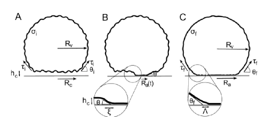
Refer to caption
Figure 2.22: Three states studied during the experiment proposed by Sengupta et al. [87]: at left, the vesicle is in a pre-nucleation state. It fluctuates at a height hcsubscript𝑐h_{c} given by a local minimum of the adhesion potential. In the middle, we see the nucleation: a part of the adhesion patch adheres strongly to the substrate, which corresponds a transition to the deep minimum of the adhesion potential. Finally, at right, we see the final strongly adhered state. The effective contact angle, here indicated by θfsubscript𝜃𝑓\theta_{f}, and the characteristic length λΛ𝜆Λ\lambda\equiv\Lambda introduced in section 1.4.3 are also represented.

From a theoretical point of view, the predicted adhesion potential for the three coatings is shown in Fig. 1.30(b) and reproduced in Fig. 2.23. For no-polymer coating, there is just a deep minimum and thus strong adhesion, while for sparse polymer coating, there is also a shallow minimum at 100nmabsent100nm\approx 100\,\mathrm{nm} corresponding to weak adhesion. For the dense polymer coating, only the shallow minimum remains and only weak adhesion is predicted. The nucleation represents thus the passage of the shallow minimum to the deeper one.
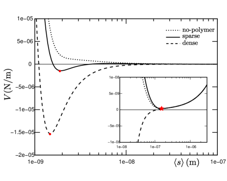
Refer to caption
Figure 2.23: Predicted adhesion potential for three different coatings. The red circles indicate the deep minima and the star indicates the shallow minimum. The curves were obtained for Rves=10μmsubscript𝑅ves10𝜇mR_{\mathrm{ves}}=10\,\mathrm{\mu m}, ster=0.2nmsubscriptster0.2nm\ell_{\mathrm{ster}}=0.2\,\mathrm{nm}, dlip=0.9nmsubscript𝑑lip0.9nmd_{\mathrm{lip}}=0.9\,\mathrm{nm}, Δρ=12.8kg/m3Δ𝜌12.8kgsuperscriptm3\Delta\rho=12.8\,\mathrm{kg/m^{3}}, AH=2×10²¹Jsubscript𝐴𝐻2superscript1021JA_{H}=2\times 10^{-21}\,\mathrm{J}, κ=100kBT𝜅100subscript𝑘B𝑇\kappa=100\,k_{\mathrm{B}}T, a=4nm𝑎4nma=4\,\mathrm{nm}, b=0.1𝑏0.1b=0.1 and Rf=87nmsubscript𝑅𝑓87nmR_{f}=87\,\mathrm{nm}.

Experimentally, as in former adhesion studies, RICM images using two different wave-lengths were used to obtain an intensity map of the adhered region. This time, however, a major improvement was introduced in the reconstruction of the height profile from these images: the case of profiles with high and variable curvature was addressed for the first time. Indeed, up to now, only the deviations caused by pure tilts and by profiles of constant curvature were accounted for. With this new method, the membrane profile was described by a succession of small curved segments and the reconstruction was made fringe by fringe (see a description of the method in [87]). The advantage of this method is that it allows a more reliable profile reconstruction even for steeper profiles, allowing thus to obtain the contact angle more precisely.

The results concerning the membrane mechanics can be summarized as follows:

  1. 1.

    Pre-nucleation state: in this state, the membranes presents strong undulations in the adhesion region. The vertical roughness ξ15nmsimilar-to-or-equalssubscript𝜉perpendicular-to15nm\xi_{\perp}\ \simeq 15\,\mathrm{nm} was measured, from which σ105N/msimilar-to𝜎superscript105Nm\sigma\sim 10^{-5}\,\mathrm{N/m} could be deduced (the relation between these quantities is given in appendix C). As Seifert had shown in his work, gravity is dominating in the case of weak adhesion, so that the tension τ𝜏\tau can be deduced from eq.(2.82), leading to τ=107106N/m𝜏superscript107superscript106Nm\tau=10^{-7}-10^{-6}\,\mathrm{N/m}. Sengupta and Limozin verified that this discrepancy is compatible with τ=σσ0𝜏𝜎subscript𝜎0\tau=\sigma-\sigma_{0} for a5nmsimilar-to𝑎5nma\sim 5\,\mathrm{nm}.

  2. 2.

    Saturation of growth of the strongly adhered patch: the vesicle gains energy by increasing the contact area. In the process, its excess are decreases up to the equilibrium represented in C of Fig. 2.22. As in micropipette experiments, the excess area before and after strong adhesion should verify eq.(2.75). This relation was verified for all vesicles studied in this work within a factor between five and ten for σ0106N/msubscript𝜎0superscript106Nm\sigma_{0}\approx 10^{-6}\,\mathrm{N/m}.

  3. 3.

    Final state of strong adhesion: instead of measuring the effective contact angle θeffsubscript𝜃eff\theta_{\mathrm{eff}} and the curvature radius Rcsubscript𝑅𝑐R_{c} as in Rädler’s work, the authors used the second method proposed in section 1.4.3 to obtain the adhesion energy WAsubscript𝑊𝐴W_{A} and the membrane tension τ𝜏\tau, by measuring the contact angle θeffsubscript𝜃eff\theta_{\mathrm{eff}} and the length λ𝜆\lambda (see Fig. 2.22). This time, the results obtained were more reliable due to the new reconstruction method and to the fact that the effective angle is more easily defined in the case of strong adhesion. From λ𝜆\lambda, the tension τ𝜏\tau could be directly derived (eq.(1.45)). Using the Young-Dupree relation and the measured values of θeffsubscript𝜃eff\theta_{\mathrm{eff}}, the adhesion energy WAsubscript𝑊𝐴W_{A} for each polymer coating could be obtained. The values obtained for WAsubscript𝑊𝐴W_{A} for the different coatings were compatible with the theoretical values, corresponding to the deep minima of the adhesion potential (see Fig. 2.23). Sadly, in this case one cannot measure neither r𝑟r nor σ𝜎\sigma by measuring the fluctuations of the membrane, since the membrane is too near to the substrate.

The results described in the points 111 and 222 are the first strong evidences in agreement with our predictions.

2.6 In a nutshell

In this chapter, we have discussed the difference between the mechanical tension τ𝜏\tau one applies through micropipettes, for instance, and the tension σ𝜎\sigma usually added to the Hamiltonian in theoretical calculations. Quantitatively, for large membranes, we have found

τ𝜏\displaystyle\tau =\displaystyle= σσ0[1σκΛ2ln(1+κΛ2σ)],𝜎subscript𝜎0delimited-[]1𝜎𝜅superscriptΛ21𝜅superscriptΛ2𝜎\displaystyle\sigma-\sigma_{0}\left[1-\frac{\sigma}{\kappa\Lambda^{2}}\ln\left(1+\frac{\kappa\Lambda^{2}}{\sigma}\right)\right]\,, (2.83)
similar-to-or-equals\displaystyle\simeq σσ0,𝜎subscript𝜎0\displaystyle\sigma-\sigma_{0}\,,

where the last approximation is valid for small tension (σ<102σr𝜎superscript102subscript𝜎𝑟\sigma<10^{-2}\,\sigma_{r}, where σr=κΛ2subscript𝜎𝑟𝜅superscriptΛ2\sigma_{r}=\kappa\Lambda^{2} is of the order of the rupture tension). The constant σ0subscript𝜎0\sigma_{0} depends only on the temperature and on the upper wave-vector cutoff ΛΛ\Lambda through

σ0=kBTΛ28π.subscript𝜎0subscript𝑘B𝑇superscriptΛ28𝜋\sigma_{0}=\frac{k_{\mathrm{B}}T\,\Lambda^{2}}{8\pi}\,. (2.84)

The cutoff ΛΛ\Lambda is related to a microscopical length of the same order of the membrane thickness. Numerically, at room temperature and assuming Λ=1/(5nm)Λ15nm\Lambda=1/(5\,\mathrm{nm}), we obtain 5×10⁶N/mabsent5superscript106Nm\approx 5\times 10^{-6}\,\mathrm{N/m}, which is a not so small. Indeed, we predict non-negligible corrections for experiments involving small tensions. We have also questioned a former demonstration asserting that the coefficient of the q2superscript𝑞2q^{2} term of the fluctuation spectrum, measured in contour analysis experiments, was equal to the mechanical tension. We have presented some results supporting our predictions: a simple numerical experiment and a recent experiment on the adhesion of GUVs.

Chapter 3 Fluctuation of forces in planar membranes

In the last chapter, we have examined the average force exerted through a cut of projected length L𝐿L on a fluctuating planar membrane

𝒇=τL𝒆x,delimited-⟨⟩𝒇𝜏𝐿subscript𝒆𝑥\langle\bm{f}\rangle=\tau\,L\,\bm{e}_{x}\,, (3.1)

where 𝒆xsubscript𝒆𝑥\bm{e}_{x} is the direction perpendicular to the cut. Using the projected stress tensor, we have obtained τ𝜏\tau as a function of the tension σ𝜎\sigma, introduced in the Hamiltonian in order to fix the average area of a membrane.

In this chapter, we would like to study the mean square deviation of this force, defined as

(Δ𝒇)2=𝒇2𝒇2.superscriptΔ𝒇2delimited-⟨⟩superscript𝒇2superscriptdelimited-⟨⟩𝒇2(\Delta\bm{f})^{2}=\langle\bm{f}^{2}\rangle-\langle\bm{f}\rangle^{2}\,. (3.2)

In the following, we will call Δ𝒇Δ𝒇\Delta\bm{f} simply the fluctuation of the force. The results exposed here were obtained in the company of Jean-Baptiste Fournier and remain unpublished. Our motivation is three-fold:

  1. 1.

    first, as experimentally one can measure the average of forces, it should also be possible to measure its fluctuations. Experimentally, for planar membranes or GUVs, this may be technically difficult, since one does not control τ𝜏\tau directly (figures are different for experiments involving membrane nanotubes, as we shall see in the following chapters). Numerically, however, it should be reasonably simple to obtain Δ𝒇Δ𝒇\Delta\bm{f} using systems similar to the one proposed in ref. [3], introduced in section 2.5.

  2. 2.

    secondly, there is no theoretical prediction on the matter. Up to now, as we have seen in last chapter, calculations on τ𝜏\tau involved differentiations of the free-energy, which is very tricky. The projected stress tensor simplifies calculations, allowing one to obtain more directly the mean square deviation of forces;

  3. 3.

    at last, this chapter is an intermediate step towards the calculation of the fluctuation of the force needed to hold a membrane nanotube, which will be done in chapter 6. Indeed, this geometry is far more interesting, presenting highly fluctuating Goldstone modes [7]. Moreover, from an experimental point of view, in order to extract or hold a tube, one applies directly a point force using optical tweezer or using magnetic beads, as we have seen in section 1.4.4. These techniques are very precise and one should thus be able to measure Δ𝒇Δ𝒇\Delta\bm{f}, even if it is of the order of some pNpN\mathrm{pN}.

In the first section, we will define precisely Δ𝒇Δ𝒇\Delta\bm{f} and remind some results obtained in the last chapter. After, in section 3.2 we shall introduce some diagrammatic tools, which are very useful since they make calculations visual. Using diagrams, one can easily identify terms whose contribution is zero and group rapidly other terms. It will prove specially useful in the calculation of the fluctuation of the force. To gain familiarity with these diagrams, we recover the result given in eq.(2.9) in section 3.3. In section 3.4, the most technical one, we shall evaluate the correlation of each term of the stress tensor. These results are finally used in section 3.5 to obtain Δ𝒇Δ𝒇\Delta\bm{f}.

3.1 Definitions and former results

Let us consider the same weakly fluctuating planar membrane described in chapter 2, whose projected area on a plane ΠΠ\Pi parallel to the average plane of the membrane is Apsubscript𝐴𝑝A_{p} (see Fig. 2.1, which we reproduce in Fig. 3.1).
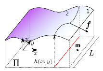
Refer to caption
Figure 3.1: Weakly fluctuating planar membrane described in the Monge’s gauge. The force 𝒇𝒇\bm{f} is exchanged through the cut of projected length L𝐿L (red). Note that we have chosen an orthonormal basis in order to have 𝒎=𝒆x𝒎subscript𝒆𝑥\bm{m}=\bm{e}_{x}.

The Hamiltonian is given by eq.(2.6) and the we remind that the corresponding correlation function reads

G(𝒓𝒓)h(𝒓)h(𝒓)=kBTAp𝒒ei𝒒(𝒓𝒓)σq2+κq4,𝐺𝒓superscript𝒓delimited-⟨⟩𝒓superscript𝒓subscript𝑘B𝑇subscript𝐴𝑝subscript𝒒superscript𝑒𝑖𝒒𝒓superscript𝒓bold-′𝜎superscript𝑞2𝜅superscript𝑞4G(\bm{r}-\bm{r}^{\prime})\equiv\langle h(\bm{r})h(\bm{r}^{\prime})\rangle=\frac{k_{\mathrm{B}}T}{A_{p}}\sum_{\bm{q}}\frac{e^{i\,\bm{q}\cdot(\bm{r}-\bm{r^{\prime}})}}{\sigma\,q^{2}+\kappa\,q^{4}}\,, (3.3)

where 𝒒=2π/Ap(m,n)𝒒2𝜋subscript𝐴𝑝𝑚𝑛\bm{q}=2\pi/\sqrt{A_{p}}(m,n) and

𝒒|n|Nmax|m|Nmaxsubscript𝒒subscript𝑛subscript𝑁maxsubscript𝑚subscript𝑁max\sum_{\bm{q}}\equiv\sum_{|n|\leq N_{\mathrm{max}}}\sum_{|m|\leq N_{\mathrm{max}}} (3.4)

with Nmax=Ap/(2πa)subscript𝑁maxsubscript𝐴𝑝2𝜋𝑎N_{\mathrm{max}}=\sqrt{A_{p}}/(2\pi a), corresponding to a maximum wave-vector qmax=1/asubscript𝑞max1𝑎q_{\mathrm{max}}=1/a, with a𝑎a a microscopical length of the order of the membrane thickness.

As shown in Fig. 3.1, we consider a cut of projected length L𝐿L parallel to 𝒆ysubscript𝒆𝑦\bm{e}_{y}. The average force exchanged through the cut is

𝒇=L(Σxx𝒆x+Σyx𝒆y+Σzx𝒆z),delimited-⟨⟩𝒇𝐿delimited-⟨⟩subscriptΣ𝑥𝑥subscript𝒆𝑥delimited-⟨⟩subscriptΣ𝑦𝑥subscript𝒆𝑦delimited-⟨⟩subscriptΣ𝑧𝑥subscript𝒆𝑧\langle\bm{f}\rangle=L\left(\langle\Sigma_{xx}\rangle\,\bm{e}_{x}+\langle\Sigma_{yx}\rangle\,\bm{e}_{y}+\langle\Sigma_{zx}\rangle\,\bm{e}_{z}\right)\,, (3.5)

where ΣijsubscriptΣ𝑖𝑗\Sigma_{ij} are the terms of the projected stress tensor for planar membranes introduced in section 1.5.2. In chapter 2, we have obtained

𝒇=(σkBT2Ap𝒒κq2σ+κq2)L𝒆x.delimited-⟨⟩𝒇𝜎subscript𝑘B𝑇2subscript𝐴𝑝subscript𝒒𝜅superscript𝑞2𝜎𝜅superscript𝑞2𝐿subscript𝒆𝑥\langle\bm{f}\rangle=\left(\sigma-\frac{k_{\mathrm{B}}T}{2A_{p}}\sum_{\bm{q}}\frac{\kappa\,q^{2}}{\sigma+\kappa\,q^{2}}\right)L\,\bm{e}_{x}\,. (3.6)

In section 3.3, we will recover this result using diagrammatic tools.

The squared fluctuation of the force is given by

(Δ𝒇)2superscriptΔ𝒇2\displaystyle(\Delta\bm{f})^{2} =\displaystyle= 𝒇2𝒇2,delimited-⟨⟩superscript𝒇2superscriptdelimited-⟨⟩𝒇2\displaystyle\langle\bm{f}^{2}\rangle-\langle\bm{f}\rangle^{2}\,, (3.7)
=\displaystyle= (Δfx)2+(Δfy)2+(Δfz)2,superscriptΔsubscript𝑓𝑥2superscriptΔsubscript𝑓𝑦2superscriptΔsubscript𝑓𝑧2\displaystyle\left(\Delta f_{x}\right)^{2}+\left(\Delta f_{y}\right)^{2}+\left(\Delta f_{z}\right)^{2}\,,

where

(Δfx)2superscriptΔsubscript𝑓𝑥2\displaystyle(\Delta f_{x})^{2} =\displaystyle= L/2L/2[Σxx(x,y)Σxx(x,y)Σxx2]𝑑y𝑑y,subscriptsuperscriptdouble-integral𝐿2𝐿2delimited-[]delimited-⟨⟩subscriptΣ𝑥𝑥𝑥𝑦subscriptΣ𝑥𝑥𝑥superscript𝑦superscriptdelimited-⟨⟩subscriptΣ𝑥𝑥2differential-d𝑦differential-dsuperscript𝑦\displaystyle\iint^{L/2}_{-L/2}\left[\,\left\langle\Sigma_{xx}(x,y)\Sigma_{xx}(x,y^{\prime})\right\rangle-\langle\Sigma_{xx}\rangle^{2}\,\right]\,dydy^{\prime}\,, (3.8)
(Δfy)2superscriptΔsubscript𝑓𝑦2\displaystyle(\Delta f_{y})^{2} =\displaystyle= L/2L/2Σyx(x,y)Σyx(x,y)𝑑y𝑑y,subscriptsuperscriptdouble-integral𝐿2𝐿2delimited-⟨⟩subscriptΣ𝑦𝑥𝑥𝑦subscriptΣ𝑦𝑥𝑥superscript𝑦differential-d𝑦differential-dsuperscript𝑦\displaystyle\iint^{L/2}_{-L/2}\left\langle\Sigma_{yx}(x,y)\Sigma_{yx}(x,y^{\prime})\right\rangle\,dydy^{\prime}\,, (3.9)
(Δfz)2superscriptΔsubscript𝑓𝑧2\displaystyle(\Delta f_{z})^{2} =\displaystyle= L/2L/2Σzx(x,y)Σzx(x,y)𝑑y𝑑y,subscriptsuperscriptdouble-integral𝐿2𝐿2delimited-⟨⟩subscriptΣ𝑧𝑥𝑥𝑦subscriptΣ𝑧𝑥𝑥superscript𝑦differential-d𝑦differential-dsuperscript𝑦\displaystyle\iint^{L/2}_{-L/2}\left\langle\Sigma_{zx}(x,y)\Sigma_{zx}(x,y^{\prime})\right\rangle\,dydy^{\prime}\,, (3.10)

are the squared fluctuation of the forces perpendicular to the cut, parallel to the cut and normal to the average membrane’s plane, respectively. Note that we have omitted Σyxdelimited-⟨⟩subscriptΣ𝑦𝑥\langle\Sigma_{yx}\rangle and Σzxdelimited-⟨⟩subscriptΣ𝑧𝑥\langle\Sigma_{zx}\rangle in eq.(3.8) and eq.(3.10), respectively, as these averages vanish (see section 2.1). The evaluation of the force fluctuation is made two steps: first, we will evaluate the correlations

Cxx(yy)subscript𝐶𝑥𝑥𝑦superscript𝑦\displaystyle C_{xx}(y-y^{\prime}) =\displaystyle= Σxx(x,y)Σxx(x,y)Σxx2,delimited-⟨⟩subscriptΣ𝑥𝑥𝑥𝑦subscriptΣ𝑥𝑥𝑥superscript𝑦superscriptdelimited-⟨⟩subscriptΣ𝑥𝑥2\displaystyle\langle\Sigma_{xx}(x,y)\Sigma_{xx}(x,y^{\prime})\rangle-\langle\Sigma_{xx}\rangle^{2}\,, (3.11)
Cyx(yy)subscript𝐶𝑦𝑥𝑦superscript𝑦\displaystyle C_{yx}(y-y^{\prime}) =\displaystyle= Σyx(x,y)Σyx(x,y),delimited-⟨⟩subscriptΣ𝑦𝑥𝑥𝑦subscriptΣ𝑦𝑥𝑥superscript𝑦\displaystyle\langle\Sigma_{yx}(x,y)\Sigma_{yx}(x,y^{\prime})\rangle\,, (3.12)
Czx(yy)subscript𝐶𝑧𝑥𝑦superscript𝑦\displaystyle C_{zx}(y-y^{\prime}) =\displaystyle= Σzx(x,y)Σzx(x,y),delimited-⟨⟩subscriptΣ𝑧𝑥𝑥𝑦subscriptΣ𝑧𝑥𝑥superscript𝑦\displaystyle\langle\Sigma_{zx}(x,y)\Sigma_{zx}(x,y^{\prime})\rangle\,, (3.13)

in section 3.4. After, in section 3.5, we will integrate these correlations twice over the cut’s length. First of all, let’s introduce some diagrammatic tools.

3.2 Diagrammatic tools

In physics, the word field is used to denote any physical quantity that varies in space. Accordingly, the height of the membrane h(𝒓)𝒓h(\bm{r}) is a field. Inspired from the Feynman diagrams used in statistical field theory, we associate graphical representations to the fields in order to make calculations visual, allowing quicker simplifications. Each field is represented by a simple straight line with a point appended to it. This point, called a vertex, represents the point 𝒓𝒓\bm{r} in which the field is evaluated. When two or more fields are evaluated at the same point, we represent them connected by the same vertex. Besides, we represent the differentiation with respect to x𝑥x or y𝑦y by a slash or a dot over the lines. We present a basic diagrammatic vocabulary in table 3.1.

Usually Diagrammatically
h(𝒓)𝒓h(\bm{r})
[Uncaptioned image]
hx(𝒓)subscript𝑥𝒓h_{x}(\bm{r})
[Uncaptioned image]
hy(𝒓)subscript𝑦𝒓h_{y}(\bm{r})
[Uncaptioned image]
h(𝒓)h(𝒓)𝒓𝒓h(\bm{r})\,h(\bm{r})
[Uncaptioned image]
h(𝒓)h(𝒓)𝒓superscript𝒓h(\bm{r})\,h(\bm{r}^{\prime})
[Uncaptioned image]
[Uncaptioned image]
Table 3.1: Basic translation rules from the usual notation into diagrams.

The thermal averages of fields are performed using Wick’s theorem, which states that the average of an even number of fields is given by the sum of all possible complete contractions. By a complete contraction, we mean linking the free ends of a set of fields, two by two, in a way that no single field remains. The continuous line formed after the contraction between two fields represents the correlation function G(𝒓)𝐺𝒓G(\bm{r}) (in this context also called propagator), suitably differentiated. If the number of fields is uneven, the theorem states that the average vanishes.

Let’s see an example of the simplest case, involving only two fields:

[Uncaptioned image]𝒓[Uncaptioned image]𝒓=[Uncaptioned image]=x|𝒓y|𝒓[G(𝒓𝒓)],delimited-⟨⟩[Uncaptioned image]𝒓[Uncaptioned image]superscript𝒓[Uncaptioned image]evaluated-atevaluated-atsubscript𝑥𝒓subscript𝑦superscript𝒓delimited-[]𝐺superscript𝒓𝒓\left\langle\begin{array}[]{c}\begin{tabular}[]{c}\includegraphics[angle={0},scale={.18}]{./figures_Chap11/simple_1.epsi}\end{tabular}\\ {}^{\bm{r}}\end{array}\begin{array}[]{c}\begin{tabular}[]{c}\includegraphics[angle={0},scale={.18}]{./figures_Chap11/simple_4.epsi}\end{tabular}\\ {}^{\bm{r}^{\prime}}\end{array}\right\rangle=\begin{tabular}[]{c}\includegraphics[angle={0},scale={.18}]{./figures_Chap11/reto_3.epsi}\end{tabular}=\partial_{x}|_{\bm{r}}\,\partial_{y}|_{\bm{r}^{\prime}}\,[G(\bm{r}^{\prime}-\bm{r})]\,, (3.14)

where x|𝒓evaluated-atsubscript𝑥𝒓\partial_{x}|_{\bm{r}} stands for the derivation with respect to x𝑥x at the point 𝒓𝒓\bm{r}. The arrow indicates that the propagator leaves at the vertex 𝒓𝒓\bm{r} and enters at the vertex 𝒓superscript𝒓\bm{r}^{\prime}. It’s direction is arbitrary: by inverting it, we would obtain x|𝒓y|𝒓[G(𝒓𝒓)]evaluated-atevaluated-atsubscript𝑥𝒓subscript𝑦superscript𝒓delimited-[]𝐺𝒓superscript𝒓\partial_{x}|_{\bm{r}}\,\partial_{y}|_{\bm{r}^{\prime}}\,[G(\bm{r}-\bm{r}^{\prime})], which yields the same result as in eq.(3.14), since G(𝒓𝒓)𝐺𝒓superscript𝒓G(\bm{r}-\bm{r}^{\prime}) is a function of |𝒓𝒓|𝒓superscript𝒓|\bm{r}-\bm{r}^{\prime}|. For the propagator given in eq.(3.3), we obtain

[Uncaptioned image]𝒓[Uncaptioned image]𝒓=kBTAp𝒒(iqx)(iqy)ei𝒒(𝒓𝒓)σq2+κq4.delimited-⟨⟩[Uncaptioned image]𝒓[Uncaptioned image]superscript𝒓subscript𝑘B𝑇subscript𝐴𝑝subscript𝒒𝑖subscript𝑞𝑥𝑖subscript𝑞𝑦superscript𝑒𝑖𝒒superscript𝒓𝒓𝜎superscript𝑞2𝜅superscript𝑞4\left\langle\begin{array}[]{c}\begin{tabular}[]{c}\includegraphics[angle={0},scale={.18}]{./figures_Chap11/simple_1.epsi}\end{tabular}\\ {}^{\bm{r}}\end{array}\begin{array}[]{c}\begin{tabular}[]{c}\includegraphics[angle={0},scale={.18}]{./figures_Chap11/simple_4.epsi}\end{tabular}\\ {}^{\bm{r}^{\prime}}\end{array}\right\rangle=\frac{k_{\mathrm{B}}T}{A_{p}}\sum_{\bm{q}}\frac{(-i\,q_{x})(i\,q_{y})\,e^{i\,\bm{q}\cdot(\bm{r}^{\prime}-\bm{r})}}{\sigma q^{2}+\kappa q^{4}}\,. (3.15)

In other words, every slash (resp.  dot) contributes to the sum a factor iqx𝑖subscript𝑞𝑥i\,q_{x} (resp. iqy𝑖subscript𝑞𝑦i\,q_{y}) if the propagator enters the vertex to which it is attached and iqx𝑖subscript𝑞𝑥-i\,q_{x} (resp. iqy𝑖subscript𝑞𝑦-i\,q_{y}) otherwise.

From this result, it is easy to show that whenever we have correlation function of the same kind of the one given in eq.(3.3), we can group slashes and dots using the following rule: in any propagator branch, one can shift a slash or a dot from one vertex side to the other if one multiplies the diagram’s coefficient by 11-1; once all derivatives are on the same side, the side matters no more. All the derivatives can be taken at the same point, contributing (iqx)𝑖subscript𝑞𝑥(i\,q_{x}) for a slash or (iqy)𝑖subscript𝑞𝑦(i\,q_{y}) for a dot, and we represent them in the center of the propagator:

[Uncaptioned image]=(1)×[Uncaptioned image]=(1)×xy[G(𝒓𝒓)].[Uncaptioned image]1[Uncaptioned image]1subscript𝑥subscript𝑦delimited-[]𝐺superscript𝒓𝒓\begin{tabular}[]{c}\includegraphics[angle={0},scale={.18}]{./figures_Chap11/reto_3.epsi}\end{tabular}=(-1)\times\begin{tabular}[]{c}\includegraphics[angle={0},scale={.18}]{./figures_Chap11/reto_4.epsi}\end{tabular}=(-1)\times\partial_{x}\partial_{y}\,[G(\bm{r}^{\prime}-\bm{r})]\,. (3.16)

As a second example, let’s see a typical case of the average of two fields evaluated at the same point. We have

[Uncaptioned image]delimited-⟨⟩[Uncaptioned image]\displaystyle\left\langle\begin{tabular}[]{c}\includegraphics[angle={0},scale={.18}]{./figures_Chap11/champ_4.epsi}\end{tabular}\right\rangle =\displaystyle= [Uncaptioned image]=(1)×[Uncaptioned image],[Uncaptioned image]1[Uncaptioned image]\displaystyle\begin{tabular}[]{c}\includegraphics[angle={0},scale={.18}]{./figures_Chap11/wick_3.epsi}\end{tabular}=(-1)\times\begin{tabular}[]{c}\includegraphics[angle={0},scale={.18}]{./figures_Chap11/wick_7.epsi}\end{tabular}\,,
=\displaystyle= yyG(𝒓),subscript𝑦𝑦𝐺𝒓\displaystyle-\partial_{yy}G(\bm{r})\,,
=\displaystyle= kBTAp𝒒(iqy)2ei𝒒𝒓σq2+κq4.subscript𝑘B𝑇subscript𝐴𝑝subscript𝒒superscript𝑖subscript𝑞𝑦2superscript𝑒𝑖𝒒𝒓𝜎superscript𝑞2𝜅superscript𝑞4\displaystyle-\frac{k_{\mathrm{B}}T}{A_{p}}\sum_{\bm{q}}\frac{(i\,q_{y})^{2}\,e^{i\,\bm{q}\cdot\bm{r}}}{\sigma q^{2}+\kappa q^{4}}\,. (3.21)

Finally, in section 3.4, we will deal with averages involving four fields. A representative example follows, where we have numbered each field to highlight all the possible complete contractions:

[Uncaptioned image]𝒓[Uncaptioned image]𝒓delimited-⟨⟩[Uncaptioned image]𝒓[Uncaptioned image]superscript𝒓\displaystyle\left\langle\begin{array}[]{c}\begin{tabular}[]{c}\includegraphics[angle={0},scale={.18}]{./figures_Chap11/champ_7_n1.epsi}\end{tabular}\\ {}^{\bm{r}}\end{array}\begin{array}[]{c}\begin{tabular}[]{c}\includegraphics[angle={0},scale={.18}]{./figures_Chap11/champ_7_n2.epsi}\end{tabular}\\ {}^{\bm{r}^{\prime}}\end{array}\right\rangle =\displaystyle= [Uncaptioned image]𝒓[Uncaptioned image]𝒓+[Uncaptioned image]+[Uncaptioned image],[Uncaptioned image]𝒓[Uncaptioned image]superscript𝒓[Uncaptioned image][Uncaptioned image]\displaystyle\begin{array}[]{c}\begin{tabular}[]{c}\includegraphics[angle={0},scale={.18}]{./figures_Chap11/wick_n1.epsi}\end{tabular}\\ {}^{\bm{r}}\end{array}\begin{array}[]{c}\begin{tabular}[]{c}\includegraphics[angle={0},scale={.18}]{./figures_Chap11/wick_n2.epsi}\end{tabular}\\ {}^{\bm{r}^{\prime}}\end{array}+\begin{tabular}[]{c}\includegraphics[angle={0},scale={.18}]{./figures_Chap11/peixe_n11.epsi}\end{tabular}+\begin{tabular}[]{c}\includegraphics[angle={0},scale={.18}]{./figures_Chap11/peixe_n21.epsi}\end{tabular}\,, (3.36)
=\displaystyle=
[Uncaptioned image]
[Uncaptioned image]
+[Uncaptioned image]+[Uncaptioned image]
,
[Uncaptioned image]
[Uncaptioned image]
[Uncaptioned image][Uncaptioned image]
\displaystyle\begin{tabular}[]{c}\includegraphics[angle={0},scale={.18}]{./figures_Chap11/wick_n1_1.epsi}\end{tabular}\begin{tabular}[]{c}\includegraphics[angle={0},scale={.18}]{./figures_Chap11/wick_n1_1.epsi}\end{tabular}+\begin{tabular}[]{c}\includegraphics[angle={0},scale={.18}]{./figures_Chap11/peixe_n1_1.epsi}\end{tabular}+\begin{tabular}[]{c}\includegraphics[angle={0},scale={.18}]{./figures_Chap11/peixe_n2_1.epsi}\end{tabular}\,,
(3.41)

which one can readily read by noting the equivalence

[Uncaptioned image]=[Uncaptioned image]×[Uncaptioned image].[Uncaptioned image][Uncaptioned image][Uncaptioned image]\begin{tabular}[]{c}\includegraphics[angle={0},scale={.18}]{./figures_Chap11/peixe_n2_1.epsi}\end{tabular}=\begin{tabular}[]{c}\includegraphics[angle={0},scale={.18}]{./figures_Chap11/reto_4.epsi}\end{tabular}\times\begin{tabular}[]{c}\includegraphics[angle={0},scale={.18}]{./figures_Chap11/reto_4.epsi}\end{tabular}\,. (3.43)

3.3 Getting familiar: evaluating 𝒇delimited-⟨⟩𝒇\langle\bm{f}\rangle with diagrammatic tools

From eq.(3.5), we see that to evaluate 𝒇delimited-⟨⟩𝒇\langle\bm{f}\rangle, one needs to evaluate the average of some component of the projected stress tensor. These components, introduced in section 1.5.2, can be written in terms of diagrams as

Σxx=σsubscriptΣ𝑥𝑥𝜎\displaystyle\Sigma_{xx}=\sigma +\displaystyle+ σ2[Uncaptioned image]σ2[Uncaptioned image]+κ2[Uncaptioned image]𝜎2[Uncaptioned image]𝜎2[Uncaptioned image]𝜅2[Uncaptioned image]\displaystyle\frac{\sigma}{2}\begin{tabular}[]{c}\includegraphics[angle={0},scale={.18}]{./figures_Chap11/champ_4.epsi}\end{tabular}-\frac{\sigma}{2}\begin{tabular}[]{c}\includegraphics[angle={0},scale={.18}]{./figures_Chap11/champ_3.epsi}\end{tabular}+\frac{\kappa}{2}\begin{tabular}[]{c}\includegraphics[angle={0},scale={.18}]{./figures_Chap11/champ_6.epsi}\end{tabular} (3.47)
\displaystyle- κ2[Uncaptioned image]+κ[Uncaptioned image]+κ[Uncaptioned image],𝜅2[Uncaptioned image]𝜅[Uncaptioned image]𝜅[Uncaptioned image]\displaystyle\frac{\kappa}{2}\begin{tabular}[]{c}\includegraphics[angle={0},scale={.18}]{./figures_Chap11/champ_5.epsi}\end{tabular}+\kappa\begin{tabular}[]{c}\includegraphics[angle={0},scale={.18}]{./figures_Chap11/champ_1.epsi}\end{tabular}+\kappa\begin{tabular}[]{c}\includegraphics[angle={0},scale={.18}]{./figures_Chap11/champ_2.epsi}\end{tabular}\,, (3.51)
Σyx=subscriptΣ𝑦𝑥absent\displaystyle\Sigma_{yx}= \displaystyle- σ[Uncaptioned image]κ[Uncaptioned image]κ[Uncaptioned image]𝜎[Uncaptioned image]𝜅[Uncaptioned image]𝜅[Uncaptioned image]\displaystyle\,\sigma\begin{tabular}[]{c}\includegraphics[angle={0},scale={.18}]{./figures_Chap11/champ_7.epsi}\end{tabular}-\kappa\begin{tabular}[]{c}\includegraphics[angle={0},scale={.18}]{./figures_Chap11/champ_8.epsi}\end{tabular}-\kappa\begin{tabular}[]{c}\includegraphics[angle={0},scale={.18}]{./figures_Chap11/champ_9.epsi}\end{tabular} (3.55)
+\displaystyle+ κ[Uncaptioned image]+κ[Uncaptioned image],𝜅[Uncaptioned image]𝜅[Uncaptioned image]\displaystyle\kappa\begin{tabular}[]{c}\includegraphics[angle={0},scale={.18}]{./figures_Chap11/champ_10.epsi}\end{tabular}+\kappa\begin{tabular}[]{c}\includegraphics[angle={0},scale={.18}]{./figures_Chap11/champ_11.epsi}\end{tabular}\,, (3.58)
Σzx=subscriptΣ𝑧𝑥absent\displaystyle\Sigma_{zx}= σ[Uncaptioned image]κ[Uncaptioned image]κ[Uncaptioned image].𝜎[Uncaptioned image]𝜅[Uncaptioned image]𝜅[Uncaptioned image]\displaystyle\sigma\begin{tabular}[]{c}\includegraphics[angle={0},scale={.18}]{./figures_Chap11/simple_1.epsi}\end{tabular}-\kappa\begin{tabular}[]{c}\includegraphics[angle={0},scale={.18}]{./figures_Chap11/simple_2.epsi}\end{tabular}-\kappa\begin{tabular}[]{c}\includegraphics[angle={0},scale={.18}]{./figures_Chap11/simple_3.epsi}\end{tabular}\,. (3.62)

The average of eq.(3.62) is the simplest one to evaluate: since each term has only an uneven number of fields, Wick’s theorem imply directly a vanishing average. We shall evaluate in details the average of ΣxxsubscriptΣ𝑥𝑥\Sigma_{xx} as an example. We have

Σxx=σdelimited-⟨⟩subscriptΣ𝑥𝑥𝜎\displaystyle\langle\Sigma_{xx}\rangle=\sigma +\displaystyle+ σ2[Uncaptioned image]σ2[Uncaptioned image]+κ2[Uncaptioned image]𝜎2[Uncaptioned image]𝜎2[Uncaptioned image]𝜅2[Uncaptioned image]\displaystyle\frac{\sigma}{2}\begin{tabular}[]{c}\includegraphics[angle={0},scale={.18}]{./figures_Chap11/wick_3.epsi}\end{tabular}-\frac{\sigma}{2}\begin{tabular}[]{c}\includegraphics[angle={0},scale={.18}]{./figures_Chap11/wick_4.epsi}\end{tabular}+\frac{\kappa}{2}\begin{tabular}[]{c}\includegraphics[angle={0},scale={.18}]{./figures_Chap11/wick_5.epsi}\end{tabular} (3.66)
\displaystyle- κ2[Uncaptioned image]+κ[Uncaptioned image]+κ[Uncaptioned image],𝜅2[Uncaptioned image]𝜅[Uncaptioned image]𝜅[Uncaptioned image]\displaystyle\frac{\kappa}{2}\begin{tabular}[]{c}\includegraphics[angle={0},scale={.18}]{./figures_Chap11/wick_6.epsi}\end{tabular}+\kappa\begin{tabular}[]{c}\includegraphics[angle={0},scale={.18}]{./figures_Chap11/wick_1.epsi}\end{tabular}+\kappa\begin{tabular}[]{c}\includegraphics[angle={0},scale={.18}]{./figures_Chap11/wick_2.epsi}\end{tabular}\,, (3.70)

where the vertex indicates the point 𝒓𝒓\bm{r} in which the average is calculated. Note that the average does not depend on it, given the isotropy of the system. Grouping the differentiations, we obtain

Σxx=σdelimited-⟨⟩subscriptΣ𝑥𝑥𝜎\displaystyle\langle\Sigma_{xx}\rangle=\sigma \displaystyle- σ2[Uncaptioned image]+σ2[Uncaptioned image]+κ2[Uncaptioned image]𝜎2[Uncaptioned image]𝜎2[Uncaptioned image]𝜅2[Uncaptioned image]\displaystyle\frac{\sigma}{2}\begin{array}[]{c}\begin{tabular}[]{c}\includegraphics[angle={0},scale={.18}]{./figures_Chap11/wick_7.epsi}\end{tabular}\end{array}+\frac{\sigma}{2}\begin{array}[]{c}\begin{tabular}[]{c}\includegraphics[angle={0},scale={.18}]{./figures_Chap11/wick_8.epsi}\end{tabular}\end{array}+\frac{\kappa}{2}\begin{array}[]{c}\begin{tabular}[]{c}\includegraphics[angle={0},scale={.18}]{./figures_Chap11/wick_9.epsi}\end{tabular}\end{array} (3.77)
\displaystyle- κ2[Uncaptioned image]κ[Uncaptioned image]κ[Uncaptioned image].𝜅2[Uncaptioned image]𝜅[Uncaptioned image]𝜅[Uncaptioned image]\displaystyle\frac{\kappa}{2}\begin{array}[]{c}\begin{tabular}[]{c}\includegraphics[angle={0},scale={.18}]{./figures_Chap11/wick_10.epsi}\end{tabular}\end{array}-\kappa\begin{array}[]{c}\begin{tabular}[]{c}\includegraphics[angle={0},scale={.18}]{./figures_Chap11/wick_10.epsi}\end{tabular}\end{array}-\kappa\begin{array}[]{c}\begin{tabular}[]{c}\includegraphics[angle={0},scale={.18}]{./figures_Chap11/wick_11.epsi}\end{tabular}\,.\end{array} (3.84)

Now, in the particular case of these diagrams, with only one vertex, we have

[Uncaptioned image]=kBTAp𝒒(iqy)2σq2+κq4=kBTAp𝒒(iqx)2σq2+κq4=[Uncaptioned image],[Uncaptioned image]subscript𝑘B𝑇subscript𝐴𝑝subscript𝒒superscript𝑖subscript𝑞𝑦2𝜎superscript𝑞2𝜅superscript𝑞4subscript𝑘B𝑇subscript𝐴𝑝subscript𝒒superscript𝑖subscript𝑞𝑥2𝜎superscript𝑞2𝜅superscript𝑞4[Uncaptioned image]\displaystyle\begin{array}[]{c}\begin{tabular}[]{c}\includegraphics[angle={0},scale={.18}]{./figures_Chap11/wick_7.epsi}\end{tabular}\end{array}=\frac{k_{\mathrm{B}}T}{A_{p}}\sum_{\bm{q}}\frac{(i\,q_{y})^{2}}{\sigma q^{2}+\kappa q^{4}}=\frac{k_{\mathrm{B}}T}{A_{p}}\sum_{\bm{q}}\frac{(i\,q_{x})^{2}}{\sigma q^{2}+\kappa q^{4}}=\begin{array}[]{c}\begin{tabular}[]{c}\includegraphics[angle={0},scale={.18}]{./figures_Chap11/wick_8.epsi}\end{tabular}\end{array}\,, (3.89)
[Uncaptioned image]=kBTAp𝒒(iqy)4σq2+κq4=kBTAp𝒒(iqx)4σq2+κq4=[Uncaptioned image].[Uncaptioned image]subscript𝑘B𝑇subscript𝐴𝑝subscript𝒒superscript𝑖subscript𝑞𝑦4𝜎superscript𝑞2𝜅superscript𝑞4subscript𝑘B𝑇subscript𝐴𝑝subscript𝒒superscript𝑖subscript𝑞𝑥4𝜎superscript𝑞2𝜅superscript𝑞4[Uncaptioned image]\displaystyle\begin{array}[]{c}\begin{tabular}[]{c}\includegraphics[angle={0},scale={.18}]{./figures_Chap11/wick_9.epsi}\end{tabular}\end{array}=\frac{k_{\mathrm{B}}T}{A_{p}}\sum_{\bm{q}}\frac{(i\,q_{y})^{4}}{\sigma q^{2}+\kappa q^{4}}=\frac{k_{\mathrm{B}}T}{A_{p}}\sum_{\bm{q}}\frac{(i\,q_{x})^{4}}{\sigma q^{2}+\kappa q^{4}}=\begin{array}[]{c}\begin{tabular}[]{c}\includegraphics[angle={0},scale={.18}]{./figures_Chap11/wick_10.epsi}\end{tabular}\end{array}\,. (3.94)

In fact, as the correlation function is calculated at 𝒓=𝒓𝒓superscript𝒓\bm{r}=\bm{r}^{\prime}, it follows that more generally we can exchange globally slashes and dots in a diagram. Sadly, this nice property does not hold for the evaluation of the kind of diagram shown in eq.(3.43), particularly important to evaluate the force fluctuation in the next section. For the present case, it follows

Σxx=σdelimited-⟨⟩subscriptΣ𝑥𝑥𝜎\displaystyle\langle\Sigma_{xx}\rangle=\sigma \displaystyle- σ2[Uncaptioned image]+σ2[Uncaptioned image]+κ2[Uncaptioned image]𝜎2[Uncaptioned image]𝜎2[Uncaptioned image]𝜅2[Uncaptioned image]\displaystyle\frac{\sigma}{2}\begin{array}[]{c}\begin{tabular}[]{c}\includegraphics[angle={0},scale={.18}]{./figures_Chap11/wick_8.epsi}\end{tabular}\end{array}+\frac{\sigma}{2}\begin{array}[]{c}\begin{tabular}[]{c}\includegraphics[angle={0},scale={.18}]{./figures_Chap11/wick_8.epsi}\end{tabular}\end{array}+\frac{\kappa}{2}\begin{array}[]{c}\begin{tabular}[]{c}\includegraphics[angle={0},scale={.18}]{./figures_Chap11/wick_10.epsi}\end{tabular}\end{array} (3.101)
\displaystyle- κ2[Uncaptioned image]κ[Uncaptioned image]κ[Uncaptioned image],𝜅2[Uncaptioned image]𝜅[Uncaptioned image]𝜅[Uncaptioned image]\displaystyle\frac{\kappa}{2}\begin{array}[]{c}\begin{tabular}[]{c}\includegraphics[angle={0},scale={.18}]{./figures_Chap11/wick_10.epsi}\end{tabular}\end{array}-\kappa\begin{array}[]{c}\begin{tabular}[]{c}\includegraphics[angle={0},scale={.18}]{./figures_Chap11/wick_10.epsi}\end{tabular}\end{array}-\kappa\begin{array}[]{c}\begin{tabular}[]{c}\includegraphics[angle={0},scale={.18}]{./figures_Chap11/wick_11.epsi}\end{tabular}\,,\end{array} (3.108)
=σabsent𝜎\displaystyle=\sigma \displaystyle- κ[Uncaptioned image]κ[Uncaptioned image],𝜅[Uncaptioned image]𝜅[Uncaptioned image]\displaystyle\kappa\begin{array}[]{c}\begin{tabular}[]{c}\includegraphics[angle={0},scale={.18}]{./figures_Chap11/wick_10.epsi}\end{tabular}\end{array}-\kappa\begin{array}[]{c}\begin{tabular}[]{c}\includegraphics[angle={0},scale={.18}]{./figures_Chap11/wick_11.epsi}\end{tabular}\,,\end{array} (3.113)

which reads

Σxxdelimited-⟨⟩subscriptΣ𝑥𝑥\displaystyle\langle\Sigma_{xx}\rangle =\displaystyle= σκkBTAp𝒒[(iqx)4+(iqx)2(iqy)2]ei𝒒(𝒓𝒓)σq2+κq4|,𝒓=𝒓\displaystyle\sigma-\frac{\kappa\,k_{\mathrm{B}}T}{A_{p}}\sum_{\bm{q}}\frac{\left[(i\,q_{x})^{4}+(i\,q_{x})^{2}(i\,q_{y})^{2}\right]\,e^{i\bm{q}(\bm{r}-\bm{r}^{\prime})}}{\sigma q^{2}+\kappa q^{4}}\left\lvert{}_{\bm{r}=\bm{r}^{\prime}}\phantom{\frac{1}{1}}\right.\,, (3.114)
=\displaystyle= σkBT2Ap𝒒κq2σ+κq2.𝜎subscript𝑘B𝑇2subscript𝐴𝑝subscript𝒒𝜅superscript𝑞2𝜎𝜅superscript𝑞2\displaystyle\sigma-\frac{k_{\mathrm{B}}T}{2\,A_{p}}\sum_{\bm{q}}\frac{\kappa\,q^{2}}{\sigma+\kappa q^{2}}\,.

As expected, we have recovered τ𝜏\tau given in eq.(2.9).

Taking into account the rules introduced in the last section, the average of ΣyxsubscriptΣ𝑦𝑥\Sigma_{yx} is very simple to evaluate. Grouping the derivatives, we have

Σyxdelimited-⟨⟩subscriptΣ𝑦𝑥\displaystyle\langle\Sigma_{yx}\rangle =\displaystyle= σ[Uncaptioned image]κ[Uncaptioned image]κ[Uncaptioned image]κ[Uncaptioned image]κ[Uncaptioned image],𝜎[Uncaptioned image]𝜅[Uncaptioned image]𝜅[Uncaptioned image]𝜅[Uncaptioned image]𝜅[Uncaptioned image]\displaystyle\sigma\begin{tabular}[]{c}\includegraphics[angle={0},scale={.18}]{./figures_Chap11/wick_n1_1.epsi}\end{tabular}-\kappa\begin{tabular}[]{c}\includegraphics[angle={0},scale={.18}]{./figures_Chap11/wick_12.epsi}\end{tabular}-\kappa\begin{tabular}[]{c}\includegraphics[angle={0},scale={.18}]{./figures_Chap11/wick_13.epsi}\end{tabular}-\kappa\begin{tabular}[]{c}\includegraphics[angle={0},scale={.18}]{./figures_Chap11/wick_12.epsi}\end{tabular}-\kappa\begin{tabular}[]{c}\includegraphics[angle={0},scale={.18}]{./figures_Chap11/wick_13.epsi}\end{tabular}\,, (3.120)
=\displaystyle= σ[Uncaptioned image]2κ[Uncaptioned image]2κ[Uncaptioned image].𝜎[Uncaptioned image]2𝜅[Uncaptioned image]2𝜅[Uncaptioned image]\displaystyle\sigma\begin{tabular}[]{c}\includegraphics[angle={0},scale={.18}]{./figures_Chap11/wick_n1_1.epsi}\end{tabular}-2\kappa\begin{tabular}[]{c}\includegraphics[angle={0},scale={.18}]{./figures_Chap11/wick_12.epsi}\end{tabular}-2\kappa\begin{tabular}[]{c}\includegraphics[angle={0},scale={.18}]{./figures_Chap11/wick_13.epsi}\end{tabular}\,. (3.124)

Let’s evaluate the first diagram:

[Uncaptioned image]=kBTAp𝒒(iqx)(iqy)σq2+κq4.[Uncaptioned image]subscript𝑘𝐵𝑇subscript𝐴𝑝subscript𝒒𝑖subscript𝑞𝑥𝑖subscript𝑞𝑦𝜎superscript𝑞2𝜅superscript𝑞4\begin{tabular}[]{c}\includegraphics[angle={0},scale={.18}]{./figures_Chap11/wick_n1_1.epsi}\end{tabular}=\frac{k_{B}T}{A_{p}}\sum_{\bm{q}}\frac{(i\,q_{x})(i\,q_{y})}{\sigma q^{2}+\kappa q^{4}}\,. (3.125)

Recalling that qx=2πm/Apsubscript𝑞𝑥2𝜋𝑚subscript𝐴𝑝q_{x}=2\pi m/\sqrt{A_{p}} and that qy=2πn/Apsubscript𝑞𝑦2𝜋𝑛subscript𝐴𝑝q_{y}=2\pi n/\sqrt{A_{p}} and that the sum over 𝒒𝒒\bm{q} stands for two sums, one on m𝑚m, and other on n𝑛n, both running from Nmaxsubscript𝑁max-N_{\mathrm{max}} up to Nmaxsubscript𝑁maxN_{\mathrm{max}}, one can readily show that the contribution of this diagram vanishes. More generally, for this kind of diagram, a uneven number of slashes or dots imply a vanishing contribution. So, we conclude that Σyx=0delimited-⟨⟩subscriptΣ𝑦𝑥0\langle\Sigma_{yx}\rangle=0 and we re-obtain the result given in eq.(3.6).

3.4 Evaluation of the projected stress tensor correlation

In this section, we will evaluate the correlation of the stress tensor at two general points over the projected cut 𝒓=x𝒆x+y𝒆y𝒓𝑥subscript𝒆𝑥𝑦subscript𝒆𝑦\bm{r}=x\,\bm{e}_{x}+y\,\bm{e}_{y} and 𝒓=x𝒆x+y𝒆ysuperscript𝒓𝑥subscript𝒆𝑥superscript𝑦subscript𝒆𝑦\bm{r}^{\prime}=x\,\bm{e}_{x}+y^{\prime}\,\bm{e}_{y}. As we discussed in section 3.2, these calculations will involve mostly diagrams of the general family

[Uncaptioned image].[Uncaptioned image]\begin{tabular}[]{c}\includegraphics[angle={0},scale={.18}]{./figures_Chap11/peixe_gen.epsi}\end{tabular}\,. (3.126)

We begin thus by reminding two properties of these diagrams:

  1. 1.

    they may be separated in two components of the form

    [Uncaptioned image]Gn,m,[Uncaptioned image]subscript𝐺𝑛𝑚\displaystyle\begin{tabular}[]{c}\includegraphics[angle={0},scale={.18}]{./figures_Chap11/reto_2.epsi}\end{tabular}\equiv G_{n,m}\,, (3.128)
    =kBTAp𝒒(i)n+mqxnqymei(yy)qyσq2+κq4,absentsubscript𝑘B𝑇subscript𝐴𝑝subscript𝒒superscript𝑖𝑛𝑚superscriptsubscript𝑞𝑥𝑛superscriptsubscript𝑞𝑦𝑚superscript𝑒𝑖𝑦superscript𝑦subscript𝑞𝑦𝜎superscript𝑞2𝜅superscript𝑞4\displaystyle=\frac{k_{\mathrm{B}}T}{A_{p}}\sum_{\bm{q}}\frac{(i)^{n+m}\,q_{x}^{n}\,q_{y}^{m}\,e^{i\,(y-y^{\prime})q_{y}}}{\sigma q^{2}+\kappa q^{4}}\,,
    =kBT(i)n+md2q(2π)2qxnqymei(yy)qyσq2+κq4,absentsubscript𝑘B𝑇superscript𝑖𝑛𝑚superscript𝑑2𝑞superscript2𝜋2superscriptsubscript𝑞𝑥𝑛superscriptsubscript𝑞𝑦𝑚superscript𝑒𝑖𝑦superscript𝑦subscript𝑞𝑦𝜎superscript𝑞2𝜅superscript𝑞4\displaystyle=k_{\mathrm{B}}T\,(i)^{n+m}\int\frac{d^{2}q}{(2\pi)^{2}}\frac{q_{x}^{n}\,q_{y}^{m}\,e^{i\,(y-y^{\prime})q_{y}}}{\sigma q^{2}+\kappa q^{4}}\,,
    =(i)n+mkBT(2π)2[0Λqn+m1σ+κq2(02πcosnθsinnθei(yy)sinθdθ)𝑑q],absentsuperscript𝑖𝑛𝑚subscript𝑘B𝑇superscript2𝜋2delimited-[]superscriptsubscript0Λsuperscript𝑞𝑛𝑚1𝜎𝜅superscript𝑞2superscriptsubscript02𝜋superscript𝑛𝜃superscript𝑛𝜃superscript𝑒𝑖𝑦superscript𝑦𝜃𝑑𝜃differential-d𝑞\displaystyle=(i)^{n+m}\frac{k_{\mathrm{B}}T}{(2\pi)^{2}}\left[\int_{0}^{\Lambda}\frac{q^{n+m-1}}{\sigma+\kappa q^{2}}\left(\int_{0}^{2\pi}\cos^{n}\theta\,\sin^{n}\theta\,e^{i\,(y-y^{\prime})\,\sin\theta}\,d\theta\right)\,dq\right]\,,
    (3.129)

    where the two last passages are good approximations for very large membranes. We remind that ΛΛ\Lambda is the upper wave-vector cutoff given by 1/a1𝑎1/a, where a𝑎a is a microscopical length of the order of the membrane thickness.

  2. 2.

    the contribution of propagators with an uneven number of slashes – and only slashes – vanishes. Indeed, one can easily proof this by remarking that the sum over 𝒒𝒒\bm{q} is symmetrical. Note that this property would not hold if we didn’t have x=x𝑥superscript𝑥x=x^{\prime}.

3.4.1 Evaluation of 𝑪𝒙𝒙subscript𝑪𝒙𝒙\bm{C_{xx}}

Let’s begin by calculating

Cxx(yy)=Σxx(x,y)Σxx(x,y)Σxx2.subscript𝐶𝑥𝑥𝑦superscript𝑦delimited-⟨⟩subscriptΣ𝑥𝑥𝑥𝑦subscriptΣ𝑥𝑥𝑥superscript𝑦superscriptdelimited-⟨⟩subscriptΣ𝑥𝑥2C_{xx}(y-y^{\prime})=\langle\Sigma_{xx}(x,y)\Sigma_{xx}(x,y^{\prime})\rangle-\langle\Sigma_{xx}\rangle^{2}\,. (3.130)

Here we can finally understand how diagrams can simplify this calculation, since normally, from eq.(3.47), one should have to evaluate about 7×7777\times 7 terms like those shown in eq.(LABEL:eq_11_avediag), implying 150absent150\approx 150 terms in total. Diagrammatically, however, many terms vanish and other can be simplified, yielding in the end

Cxx(yy)subscript𝐶𝑥𝑥𝑦superscript𝑦\displaystyle C_{xx}(y-y^{\prime}) =\displaystyle= σ22[Uncaptioned image]+σ22[Uncaptioned image]σκ[Uncaptioned image]superscript𝜎22[Uncaptioned image]superscript𝜎22[Uncaptioned image]𝜎𝜅[Uncaptioned image]\displaystyle\frac{\sigma^{2}}{2}\begin{tabular}[]{c}\includegraphics[angle={0},scale={.115}]{./figures_Chap11/peixe_1.epsi}\end{tabular}+\frac{\sigma^{2}}{2}\begin{tabular}[]{c}\includegraphics[angle={0},scale={.115}]{./figures_Chap11/peixe_2.epsi}\end{tabular}-\sigma\kappa\begin{tabular}[]{c}\includegraphics[angle={0},scale={.115}]{./figures_Chap11/peixe_3.epsi}\end{tabular} (3.134)
+\displaystyle+ σκ[Uncaptioned image]2σκ[Uncaptioned image]2σκ[Uncaptioned image]𝜎𝜅[Uncaptioned image]2𝜎𝜅[Uncaptioned image]2𝜎𝜅[Uncaptioned image]\displaystyle\sigma\kappa\begin{tabular}[]{c}\includegraphics[angle={0},scale={.115}]{./figures_Chap11/peixe_4.epsi}\end{tabular}-2\sigma\kappa\begin{tabular}[]{c}\includegraphics[angle={0},scale={.115}]{./figures_Chap11/peixe_8.epsi}\end{tabular}-2\sigma\kappa\begin{tabular}[]{c}\includegraphics[angle={0},scale={.115}]{./figures_Chap11/peixe_9.epsi}\end{tabular} (3.138)
+\displaystyle+ κ22[Uncaptioned image]+3κ22[Uncaptioned image]+2κ2[Uncaptioned image]superscript𝜅22[Uncaptioned image]3superscript𝜅22[Uncaptioned image]2superscript𝜅2[Uncaptioned image]\displaystyle\frac{\kappa^{2}}{2}\begin{tabular}[]{c}\includegraphics[angle={0},scale={.115}]{./figures_Chap11/peixe_7.epsi}\end{tabular}+\frac{3\,\kappa^{2}}{2}\begin{tabular}[]{c}\includegraphics[angle={0},scale={.115}]{./figures_Chap11/peixe_5.epsi}\end{tabular}+2\kappa^{2}\begin{tabular}[]{c}\includegraphics[angle={0},scale={.115}]{./figures_Chap11/peixe_6.epsi}\end{tabular} (3.142)
+\displaystyle+ κ2[Uncaptioned image]+2κ2[Uncaptioned image]+κ2[Uncaptioned image].superscript𝜅2[Uncaptioned image]2superscript𝜅2[Uncaptioned image]superscript𝜅2[Uncaptioned image]\displaystyle\kappa^{2}\begin{tabular}[]{c}\includegraphics[angle={0},scale={.115}]{./figures_Chap11/peixe_11.epsi}\end{tabular}+2\kappa^{2}\begin{tabular}[]{c}\includegraphics[angle={0},scale={.115}]{./figures_Chap11/peixe_10.epsi}\end{tabular}+\kappa^{2}\begin{tabular}[]{c}\includegraphics[angle={0},scale={.115}]{./figures_Chap11/peixe_12.epsi}\end{tabular}\,. (3.146)

In terms of the Gn,msubscript𝐺𝑛𝑚G_{n,m} defined in eq.(3.128), we obtain

Cxx(yy)subscript𝐶𝑥𝑥𝑦superscript𝑦\displaystyle C_{xx}(y-y^{\prime}) =\displaystyle= σ22(G2,02+G0,22)σκ(G2,12G0,32)2σκG2,0(G4,0+G2,2)superscript𝜎22superscriptsubscript𝐺202superscriptsubscript𝐺022𝜎𝜅superscriptsubscript𝐺212superscriptsubscript𝐺0322𝜎𝜅subscript𝐺20subscript𝐺40subscript𝐺22\displaystyle\frac{\sigma^{2}}{2}\left(G_{2,0}^{2}+G_{0,2}^{2}\right)-\sigma\kappa\left(G_{2,1}^{2}-G_{0,3}^{2}\right)-2\sigma\kappa\,G_{2,0}\left(G_{4,0}+G_{2,2}\right)
+\displaystyle+ κ22(G0,42+3G4,02+4G4,0G2,2)+κ2G2,0(G6,0+2G4,2+G2,4).superscript𝜅22superscriptsubscript𝐺0423superscriptsubscript𝐺4024subscript𝐺40subscript𝐺22superscript𝜅2subscript𝐺20subscript𝐺602subscript𝐺42subscript𝐺24\displaystyle\frac{\kappa^{2}}{2}\left(G_{0,4}^{2}+3\,G_{4,0}^{2}+4\,G_{4,0}\,G_{2,2}\right)+\kappa^{2}\,G_{2,0}\left(G_{6,0}+2\,G_{4,2}+G_{2,4}\right)\,.

Considering very large membranes and performing the angular integral in eq.(3.129) for each Gn,msubscript𝐺𝑛𝑚G_{n,m}, eq.(LABEL:eq_11_Cxx_G) becomes

Cxx(yy)subscript𝐶𝑥𝑥𝑦superscript𝑦\displaystyle C_{xx}(y-y^{\prime}) =\displaystyle= σ2[12B212(Y)1YB10(Y)B21(Y)+1Y2B102(Y)]superscript𝜎2delimited-[]12superscriptsubscript𝐵212𝑌1𝑌subscript𝐵10𝑌subscript𝐵21𝑌1superscript𝑌2superscriptsubscript𝐵102𝑌\displaystyle\sigma^{2}\left[\frac{1}{2}\,B_{21}^{2}(Y)-\frac{1}{Y}\,B_{10}(Y)\,B_{21}(Y)+\frac{1}{Y^{2}}\,B_{10}^{2}(Y)\right] (3.149)
+\displaystyle+ σκ[B122(Y)2YB12(Y)B21(Y)+2Y2B10(Y)B12(Y)]𝜎𝜅delimited-[]superscriptsubscript𝐵122𝑌2𝑌subscript𝐵12𝑌subscript𝐵21𝑌2superscript𝑌2subscript𝐵10𝑌subscript𝐵12𝑌\displaystyle\sigma\kappa\,\left[B_{12}^{2}(Y)-\frac{2}{Y}\,B_{12}(Y)\,B_{21}(Y)+\frac{2}{Y^{2}}\,B_{10}(Y)\,B_{12}(Y)\right]
+\displaystyle+ κ2[12B032(Y)2YB03(Y)B12(Y)+2Y2B122(Y)\displaystyle\kappa^{2}\left[\frac{1}{2}\,B_{03}^{2}(Y)-\frac{2}{Y}\,B_{03}(Y)\,B_{12}(Y)+\frac{2}{Y^{2}}\,B_{12}^{2}(Y)\right.
+\displaystyle+ 1Y2B10(Y)B14(Y)+3Y2B03(Y)B21(Y)],\displaystyle\left.\frac{1}{Y^{2}}\,B_{10}(Y)\,B_{14}(Y)+\frac{3}{Y^{2}}\,B_{03}(Y)\,B_{21}(Y)\right]\,,

where Y=|yy|𝑌𝑦superscript𝑦Y=|y-y^{\prime}| and

Bij(y)=kBT0Λdq2πqjJi(qy)σ+κq2,subscript𝐵𝑖𝑗𝑦subscript𝑘B𝑇superscriptsubscript0Λ𝑑𝑞2𝜋superscript𝑞𝑗subscript𝐽𝑖𝑞𝑦𝜎𝜅superscript𝑞2B_{ij}(y)={k_{\mathrm{B}}T}\int_{0}^{\Lambda}\frac{dq}{2\pi}\frac{q^{j}\,J_{i}(q\,y)}{\sigma+\kappa q^{2}}\,, (3.150)

with Jisubscript𝐽𝑖J_{i} standing for the first kind Bessel function of order i𝑖i. Note that, as expected given the isotropy of the system, Cxxsubscript𝐶𝑥𝑥C_{xx} depends only on the distance between the points. At this point, it is useful to rewrite eq.(3.150):

Bij(y)=kBTκΛj101dq2πqjJi(qΛy)r+q2=kBTκΛj1B~ij(Λy),subscript𝐵𝑖𝑗𝑦subscript𝑘B𝑇𝜅superscriptΛ𝑗1superscriptsubscript01𝑑𝑞2𝜋superscript𝑞𝑗subscript𝐽𝑖𝑞Λ𝑦𝑟superscript𝑞2subscript𝑘B𝑇𝜅superscriptΛ𝑗1subscript~𝐵𝑖𝑗Λ𝑦B_{ij}(y)=\frac{k_{\mathrm{B}}T}{\kappa}\,\Lambda^{j-1}\,\int_{0}^{1}\frac{dq}{2\pi}\frac{q^{j}\,J_{i}(q\,\Lambda\,y)}{r+q^{2}}=\frac{k_{\mathrm{B}}T}{\kappa}\,\Lambda^{j-1}\,\tilde{B}_{ij}(\Lambda y)\,, (3.151)

where B~ijsubscript~𝐵𝑖𝑗\tilde{B}_{ij} is dimensionless. To simplify notations, we have omitted the dependence of B~ijsubscript~𝐵𝑖𝑗\tilde{B}_{ij} on r𝑟r, given by

r=σκΛ2=σσr,𝑟𝜎𝜅superscriptΛ2𝜎subscript𝜎𝑟r=\frac{\sigma}{\kappa\Lambda^{2}}=\frac{\sigma}{\sigma_{r}}\,, (3.152)

with σrsubscript𝜎𝑟\sigma_{r} of the order of the membrane rupture tension. Eq.(3.149) can be rewritten as

Cxx(yy)subscript𝐶𝑥𝑥𝑦superscript𝑦\displaystyle C_{xx}(y-y^{\prime}) =\displaystyle= 64π2σ02{r2[12B~212(ΛY)B~10(ΛY)B~21(ΛY)ΛY+B~102(ΛY)(ΛY)2]\displaystyle 64\pi^{2}\sigma_{0}^{2}\left\{r^{2}\left[\frac{1}{2}\,\tilde{B}_{21}^{2}(\Lambda Y)-\frac{\tilde{B}_{10}(\Lambda Y)\,\tilde{B}_{21}(\Lambda Y)}{\Lambda Y}+\frac{\tilde{B}_{10}^{2}(\Lambda Y)}{(\Lambda Y)^{2}}\right]\right. (3.153)
+\displaystyle+ r[B~122(ΛY)2B~12(Y)B~21(ΛY)ΛY+2B~10(ΛY)B~12(ΛY)(ΛY)2]𝑟delimited-[]superscriptsubscript~𝐵122Λ𝑌2subscript~𝐵12𝑌subscript~𝐵21Λ𝑌Λ𝑌2subscript~𝐵10Λ𝑌subscript~𝐵12Λ𝑌superscriptΛ𝑌2\displaystyle r\,\left[\tilde{B}_{12}^{2}(\Lambda Y)-2\,\frac{\tilde{B}_{12}(Y)\,\tilde{B}_{21}(\Lambda Y)}{\Lambda Y}+2\,\frac{\tilde{B}_{10}(\Lambda Y)\,\tilde{B}_{12}(\Lambda Y)}{(\Lambda Y)^{2}}\right]
+\displaystyle+ [12B~032(ΛY)2B~03(ΛY)B~12(ΛY)ΛY+2B~122(ΛY)(ΛY)2\displaystyle\left[\frac{1}{2}\,\tilde{B}_{03}^{2}(\Lambda Y)-2\,\frac{\tilde{B}_{03}(\Lambda Y)\,\tilde{B}_{12}(\Lambda Y)}{\Lambda Y}+2\,\frac{\tilde{B}_{12}^{2}(\Lambda Y)}{(\Lambda Y)^{2}}\right.
+\displaystyle+ B~10(ΛY)B~14(ΛY)(ΛY)2+3B~03(ΛY)B~21(ΛY)(ΛY)2]},\displaystyle\left.\left.\frac{\tilde{B}_{10}(\Lambda Y)\,\tilde{B}_{14}(\Lambda Y)}{(\Lambda Y)^{2}}+3\,\frac{\tilde{B}_{03}(\Lambda Y)\,\tilde{B}_{21}(\Lambda Y)}{(\Lambda Y)^{2}}\right]\right\}\,,

where

σ0=κΛ28πβκsubscript𝜎0𝜅superscriptΛ28𝜋𝛽𝜅\sigma_{0}=\frac{\kappa\Lambda^{2}}{8\pi\beta\kappa} (3.154)

was already introduced in the last chapter. Note that the terms inside the brackets are dimensionless and that Cxxsubscript𝐶𝑥𝑥C_{xx} depends actually only on σ0subscript𝜎0\sigma_{0}, on r𝑟r and on ΛY|yy|/aΛ𝑌𝑦superscript𝑦𝑎\Lambda Y\equiv|y-y^{\prime}|/a.

In Fig.(3.2) we can see Cxxsubscript𝐶𝑥𝑥C_{xx} as a function of Y𝑌Y in units of a𝑎a for different tensions. These curves were normalized by

Cxx(0)=(σ022){3+[14r+3r2ln(1+1r)]ln(1+1r)},subscript𝐶𝑥𝑥0superscriptsubscript𝜎0223delimited-[]14𝑟3superscript𝑟211𝑟11𝑟C_{xx}(0)=\left(\frac{\sigma_{0}^{2}}{2}\right)\left\{3+\left[1-4r+3r^{2}\ln\left(1+\frac{1}{r}\right)\right]\ln\left(1+\frac{1}{r}\right)\right\}\,, (3.155)

which we have obtained analytically from eq.(3.153).
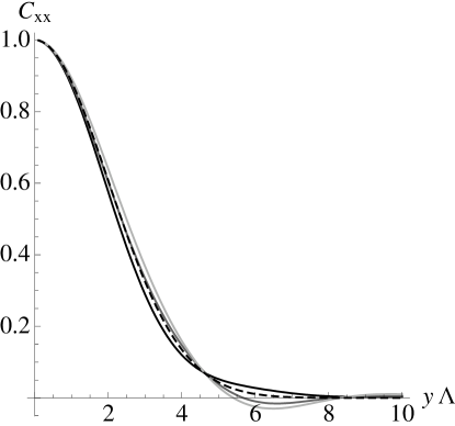
Refer to caption
Figure 3.2: Plot of the correlation of ΣxxsubscriptΣ𝑥𝑥\Sigma_{xx} as a function of the distance in units of the microscopical length a=Λ1𝑎superscriptΛ1a=\Lambda^{-1} (normalized by the auto-correlation given in eq.(3.155)). The black line stands for r=1𝑟1r=1, the dark gray corresponds to r=102𝑟superscript102r=10^{-2} and the light gray corresponds to r=104𝑟superscript104r=10^{-4}. For κ25kBT𝜅25subscript𝑘B𝑇\kappa\approx 25\,k_{\mathrm{B}}T, it corresponds to σ=4×10³N/m𝜎4superscript103Nm\sigma=4\times 10^{-3}\,\mathrm{N/m}, σ=4×10⁵N/m𝜎4superscript105Nm\sigma=4\times 10^{-5}\,\mathrm{N/m} and σ=4×10⁷N/m𝜎4superscript107Nm\sigma=4\times 10^{-7}\,\mathrm{N/m}, respectively. The dashed line shows that in any case, the curves are well approximated by the Gaussian e(ΛY)2/8superscript𝑒superscriptΛ𝑌28e^{-(\Lambda Y)^{2}/8}.

First of all, we notice that the curves do almost not depend on r𝑟r – and consequently on the tension. Accordingly, the decrease of the correlation is dominated by the bending rigidity, which is not evident, since the Σxxdelimited-⟨⟩subscriptΣ𝑥𝑥\langle\Sigma_{xx}\rangle depends strongly on the tension. Secondly, Cxxsubscript𝐶𝑥𝑥C_{xx} decreases relatively fast: about five times the microscopical length a𝑎a for any tension. At last, in the following we will need to integrate Cxxsubscript𝐶𝑥𝑥C_{xx}. It will be thus useful to remark that for any tension, it is very well approximated by

Cxx(yy)Cxx(0)eΛ2(yy)28.similar-to-or-equalssubscript𝐶𝑥𝑥𝑦superscript𝑦subscript𝐶𝑥𝑥0superscript𝑒superscriptΛ2superscript𝑦superscript𝑦28C_{xx}(y-y^{\prime})\simeq C_{xx}(0)\,e^{-\frac{\Lambda^{2}\,(y-y^{\prime})^{2}}{8}}\,. (3.156)
3.4.2 Evaluation of 𝑪𝒚𝒙subscript𝑪𝒚𝒙\bm{C_{yx}}

Following the same route as in the last section,

Cyx(yy)Σyx(x,y)Σyx(x,y)subscript𝐶𝑦𝑥𝑦superscript𝑦delimited-⟨⟩subscriptΣ𝑦𝑥𝑥𝑦subscriptΣ𝑦𝑥𝑥superscript𝑦C_{yx}(y-y^{\prime})\equiv\langle\Sigma_{yx}(x,y)\,\Sigma_{yx}(x,y^{\prime})\rangle (3.157)

can be written in terms of diagrams as

Cyx(yy)subscript𝐶𝑦𝑥𝑦superscript𝑦\displaystyle C_{yx}(y-y^{\prime}) =\displaystyle= σ2[Uncaptioned image]2σκ[Uncaptioned image]2σκ[Uncaptioned image]superscript𝜎2[Uncaptioned image]2𝜎𝜅[Uncaptioned image]2𝜎𝜅[Uncaptioned image]\displaystyle\sigma^{2}\begin{tabular}[]{c}\includegraphics[angle={0},scale={.115}]{./figures_Chap11/peixe_13.epsi}\end{tabular}-2\sigma\kappa\begin{tabular}[]{c}\includegraphics[angle={0},scale={.115}]{./figures_Chap11/peixe_21.epsi}\end{tabular}-2\sigma\kappa\begin{tabular}[]{c}\includegraphics[angle={0},scale={.115}]{./figures_Chap11/peixe_22.epsi}\end{tabular} (3.161)
+\displaystyle+ 2σκ[Uncaptioned image]+2σκ[Uncaptioned image]2κ2[Uncaptioned image]2𝜎𝜅[Uncaptioned image]2𝜎𝜅[Uncaptioned image]2superscript𝜅2[Uncaptioned image]\displaystyle 2\sigma\kappa\begin{tabular}[]{c}\includegraphics[angle={0},scale={.115}]{./figures_Chap11/peixe_3.epsi}\end{tabular}+2\sigma\kappa\begin{tabular}[]{c}\includegraphics[angle={0},scale={.115}]{./figures_Chap11/peixe_23.epsi}\end{tabular}-2\kappa^{2}\begin{tabular}[]{c}\includegraphics[angle={0},scale={.115}]{./figures_Chap11/peixe_17.epsi}\end{tabular} (3.165)
\displaystyle- 2κ2[Uncaptioned image]2κ2[Uncaptioned image]2κ2[Uncaptioned image]2superscript𝜅2[Uncaptioned image]2superscript𝜅2[Uncaptioned image]2superscript𝜅2[Uncaptioned image]\displaystyle 2\kappa^{2}\begin{tabular}[]{c}\includegraphics[angle={0},scale={.115}]{./figures_Chap11/peixe_18.epsi}\end{tabular}-2\kappa^{2}\begin{tabular}[]{c}\includegraphics[angle={0},scale={.115}]{./figures_Chap11/peixe_24.epsi}\end{tabular}-2\kappa^{2}\begin{tabular}[]{c}\includegraphics[angle={0},scale={.115}]{./figures_Chap11/peixe_25.epsi}\end{tabular} (3.169)
+\displaystyle+ κ2[Uncaptioned image]+2κ2[Uncaptioned image]+κ2[Uncaptioned image]superscript𝜅2[Uncaptioned image]2superscript𝜅2[Uncaptioned image]superscript𝜅2[Uncaptioned image]\displaystyle\kappa^{2}\begin{tabular}[]{c}\includegraphics[angle={0},scale={.115}]{./figures_Chap11/peixe_6.epsi}\end{tabular}+2\kappa^{2}\begin{tabular}[]{c}\includegraphics[angle={0},scale={.115}]{./figures_Chap11/peixe_15.epsi}\end{tabular}+\kappa^{2}\begin{tabular}[]{c}\includegraphics[angle={0},scale={.115}]{./figures_Chap11/peixe_16.epsi}\end{tabular} (3.173)
+\displaystyle+ κ2[Uncaptioned image]+2κ2[Uncaptioned image]+κ2[Uncaptioned image],superscript𝜅2[Uncaptioned image]2superscript𝜅2[Uncaptioned image]superscript𝜅2[Uncaptioned image]\displaystyle\kappa^{2}\begin{tabular}[]{c}\includegraphics[angle={0},scale={.115}]{./figures_Chap11/peixe_26.epsi}\end{tabular}+2\kappa^{2}\begin{tabular}[]{c}\includegraphics[angle={0},scale={.115}]{./figures_Chap11/peixe_27.epsi}\end{tabular}+\kappa^{2}\begin{tabular}[]{c}\includegraphics[angle={0},scale={.115}]{./figures_Chap11/peixe_28.epsi}\end{tabular}\,, (3.177)

which reads

Cyx(yy)subscript𝐶𝑦𝑥𝑦superscript𝑦\displaystyle C_{yx}(y-y^{\prime}) =\displaystyle= σ2G0,2G2,0+2σκ[G2,1(G2,1+G0,3)G0,2(G4,0+G2,2)]superscript𝜎2subscript𝐺02subscript𝐺202𝜎𝜅delimited-[]subscript𝐺21subscript𝐺21subscript𝐺03subscript𝐺02subscript𝐺40subscript𝐺22\displaystyle\sigma^{2}\,G_{0,2}\,G_{2,0}+2\sigma\kappa\left[G_{2,1}\left(G_{2,1}+G_{0,3}\right)-G_{0,2}\left(G_{4,0}+G_{2,2}\right)\right]
\displaystyle- 2κ2(G2,1+G0,3)(G4,1+G2,3)+κ2G2,2(G4,0+2G2,2+G0,4)2superscript𝜅2subscript𝐺21subscript𝐺03subscript𝐺41subscript𝐺23superscript𝜅2subscript𝐺22subscript𝐺402subscript𝐺22subscript𝐺04\displaystyle 2\,\kappa^{2}\left(G_{2,1}+G_{0,3}\right)\left(G_{4,1}+G_{2,3}\right)+\kappa^{2}\,G_{2,2}\left(G_{4,0}+2\,G_{2,2}+G_{0,4}\right)
+\displaystyle+ κ2G0,2(G6,0+2G4,2+G2,4).superscript𝜅2subscript𝐺02subscript𝐺602subscript𝐺42subscript𝐺24\displaystyle\kappa^{2}\,G_{0,2}\,\left(G_{6,0}+2\,G_{4,2}+G_{2,4}\right)\,.

In the thermodynamical limit, we obtain

Cyx(yy)subscript𝐶𝑦𝑥𝑦superscript𝑦\displaystyle C_{yx}(y-y^{\prime}) =\displaystyle= 64π2σ02{r2[B~102(ΛY)(ΛY)2B~10(ΛY)B~21(ΛY)ΛY]+2rB~10(ΛY)B~12(ΛY)(ΛY)2\displaystyle 64\pi^{2}\sigma_{0}^{2}\left\{r^{2}\,\left[\frac{\tilde{B}_{10}^{2}(\Lambda Y)}{(\Lambda Y)^{2}}-\frac{\tilde{B}_{10}(\Lambda Y)\,\tilde{B}_{21}(\Lambda Y)}{\Lambda Y}\right]+2r\,\frac{\tilde{B}_{10}(\Lambda Y)\,\tilde{B}_{12}(\Lambda Y)}{(\Lambda Y)^{2}}\right. (3.180)
+\displaystyle+ [2B~12(ΛY)B~23(ΛY)ΛYB~03(ΛY)B~32(ΛY)ΛYB~21(ΛY)B~14(ΛY)ΛY\displaystyle\left[2\,\frac{\tilde{B}_{12}(\Lambda Y)\,\tilde{B}_{23}(\Lambda Y)}{\Lambda Y}-\frac{\tilde{B}_{03}(\Lambda Y)\,\tilde{B}_{32}(\Lambda Y)}{\Lambda Y}-\frac{\tilde{B}_{21}(\Lambda Y)\,\tilde{B}_{14}(\Lambda Y)}{\Lambda Y}\right.
+\displaystyle+ B~03(ΛY)B~21(ΛY)(ΛY)2+B~10(ΛY)B~14(ΛY)(ΛY)2]},\displaystyle\left.\left.\frac{\tilde{B}_{03}(\Lambda Y)\,\tilde{B}_{21}(\Lambda Y)}{(\Lambda Y)^{2}}+\frac{\tilde{B}_{10}(\Lambda Y)\,\tilde{B}_{14}(\Lambda Y)}{(\Lambda Y)^{2}}\right]\right\}\,,

where Y=|yy|𝑌𝑦superscript𝑦Y=|y-y^{\prime}| and B~ijsubscript~𝐵𝑖𝑗\tilde{B}_{ij} is defined in eq.(3.151).

At last, we show in Fig. 3.3 the behavior of Cyxsubscript𝐶𝑦𝑥C_{yx} normalized by the auto-correlation

Cyx(0)=(σ022){1+[1+r2ln(1+1r)]ln(1+1r)},subscript𝐶𝑦𝑥0superscriptsubscript𝜎0221delimited-[]1superscript𝑟211𝑟11𝑟C_{yx}(0)=\left(\frac{\sigma_{0}^{2}}{2}\right)\left\{1+\left[1+r^{2}\ln\left(1+\frac{1}{r}\right)\right]\ln\left(1+\frac{1}{r}\right)\right\}\,, (3.181)

obtained analytically from eq.(3.180).
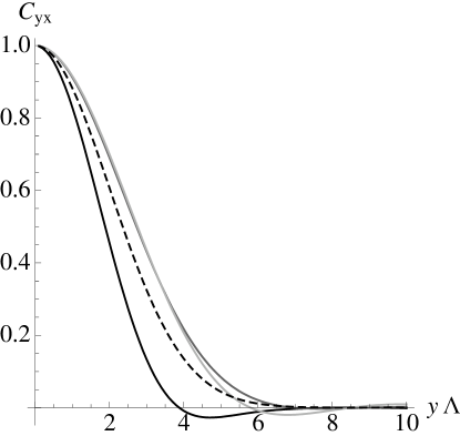
Refer to caption

Figure 3.3: Plot of the normalized correlation of the transverse component of the stress tensor for different values of r𝑟r as a function of the distance in units of Λ1superscriptΛ1\Lambda^{-1}. The black line corresponds to r=1𝑟1r=1, dark gray corresponds to r=102𝑟superscript102r=10^{-2} and light gray corresponds to r=104𝑟superscript104r=10^{-4}. For κ25kBT𝜅25subscript𝑘B𝑇\kappa\approx 25\,k_{\mathrm{B}}T, it corresponds to σ=4×10³N/m𝜎4superscript103Nm\sigma=4\times 10^{-3}\,\mathrm{N/m}, σ=4×10⁵N/m𝜎4superscript105Nm\sigma=4\times 10^{-5}\,\mathrm{N/m} and σ=4×10⁷N/m𝜎4superscript107Nm\sigma=4\times 10^{-7}\,\mathrm{N/m}, respectively. The dashed line shows a rough Gaussian approximation.

The correlation Cyxsubscript𝐶𝑦𝑥C_{yx} is very similar to Cxxsubscript𝐶𝑥𝑥C_{xx}, sharing with it three features:

  1. 1.

    as before, Cyxsubscript𝐶𝑦𝑥C_{yx} normalized by the auto-correlation depends only weakly on the tension, specially in the regime of low tensions. The shape of the correlation is dominated by the bending rigidity;

  2. 2.

    Cyxsubscript𝐶𝑦𝑥C_{yx} relaxes over approximately five times the microscopical length a𝑎a;

  3. 3.

    the same approximation

    Cyx(yy)Cyx(0)eΛ2(yy)28similar-to-or-equalssubscript𝐶𝑦𝑥𝑦superscript𝑦subscript𝐶𝑦𝑥0superscript𝑒superscriptΛ2superscript𝑦superscript𝑦28C_{yx}(y-y^{\prime})\simeq C_{yx}(0)\,e^{-\frac{\Lambda^{2}(y-y^{\prime})^{2}}{8}} (3.182)

    holds, although it is less good.

3.4.3 Evaluation of 𝑪𝒛𝒙subscript𝑪𝒛𝒙\bm{C_{zx}}

The correlation of the normal component

Czx(yy)=Σzx(x,y)Σzx(x,y)subscript𝐶𝑧𝑥𝑦superscript𝑦delimited-⟨⟩subscriptΣ𝑧𝑥𝑥𝑦subscriptΣ𝑧𝑥𝑥superscript𝑦C_{zx}(y-y^{\prime})=\langle\Sigma_{zx}(x,y)\,\Sigma_{zx}(x,y^{\prime})\rangle (3.183)

is the simplest one to evaluate. Diagrammatically, we have

Czx(yy)=subscript𝐶𝑧𝑥𝑦superscript𝑦absent\displaystyle C_{zx}(y-y^{\prime})= \displaystyle- σ2[Uncaptioned image]+2σκ[Uncaptioned image]+2σκ[Uncaptioned image]superscript𝜎2[Uncaptioned image]2𝜎𝜅[Uncaptioned image]2𝜎𝜅[Uncaptioned image]\displaystyle\sigma^{2}\begin{tabular}[]{c}\includegraphics[angle={0},scale={.13}]{./figures_Chap11/ligne_1.epsi}\end{tabular}+2\sigma\kappa\begin{tabular}[]{c}\includegraphics[angle={0},scale={.13}]{./figures_Chap11/ligne_2.epsi}\end{tabular}+2\sigma\kappa\begin{tabular}[]{c}\includegraphics[angle={0},scale={.13}]{./figures_Chap11/ligne_3.epsi}\end{tabular} (3.187)
\displaystyle- κ2[Uncaptioned image]2κ2[Uncaptioned image]κ2[Uncaptioned image],superscript𝜅2[Uncaptioned image]2superscript𝜅2[Uncaptioned image]superscript𝜅2[Uncaptioned image]\displaystyle\kappa^{2}\begin{tabular}[]{c}\includegraphics[angle={0},scale={.13}]{./figures_Chap11/ligne_4.epsi}\end{tabular}-2\kappa^{2}\begin{tabular}[]{c}\includegraphics[angle={0},scale={.13}]{./figures_Chap11/ligne_5.epsi}\end{tabular}-\kappa^{2}\phantom{1}\begin{tabular}[]{c}\includegraphics[angle={0},scale={.13}]{./figures_Chap11/ligne_6.epsi}\end{tabular}\,,
=\displaystyle= σ2G2,0+2σκ(G4,0+G2,2)κ2(G6,0+2G4,2+G2,4).superscript𝜎2subscript𝐺202𝜎𝜅subscript𝐺40subscript𝐺22superscript𝜅2subscript𝐺602subscript𝐺42subscript𝐺24\displaystyle-\sigma^{2}\,G_{2,0}+2\sigma\kappa\left(G_{4,0}+G_{2,2}\right)-\kappa^{2}\left(G_{6,0}+2G_{4,2}+G_{2,4}\right)\,.

This time, in the thermodynamical limit, one can integrate Czxsubscript𝐶𝑧𝑥C_{zx} not only over the angular coordinate, but also over q𝑞q, obtaining

Czx(yy)=32πβκσ02{r[1J0(ΛY)]+J2(ΛY)(ΛY)2},subscript𝐶𝑧𝑥𝑦superscript𝑦32𝜋𝛽𝜅superscriptsubscript𝜎02𝑟delimited-[]1subscript𝐽0Λ𝑌subscript𝐽2Λ𝑌superscriptΛ𝑌2C_{zx}(y-y^{\prime})=32\pi\beta\kappa\,\sigma_{0}^{2}\left\{\frac{r\left[1-J_{0}(\Lambda Y)\right]+J_{2}(\Lambda Y)}{(\Lambda Y)^{2}}\right\}\,, (3.193)

and accordingly

Czx(0)=8πβκ(σ022)(1+2r).subscript𝐶𝑧𝑥08𝜋𝛽𝜅superscriptsubscript𝜎02212𝑟C_{zx}(0)=8\pi\beta\kappa\,\left(\frac{\sigma_{0}^{2}}{2}\right)\left(1+2\,r\right)\,. (3.194)

As we can see in Fig. 3.4, Czxsubscript𝐶𝑧𝑥C_{zx} normalized by Czx(0)subscript𝐶𝑧𝑥0C_{zx}(0) has roughly the same be features of the former correlations: it does almost not depend on the tension and it becomes negligible for distances bigger than 5aabsent5𝑎\approx 5\,a. This time, however, as Czxsubscript𝐶𝑧𝑥C_{zx} is very simple, directly given by an analytical function.
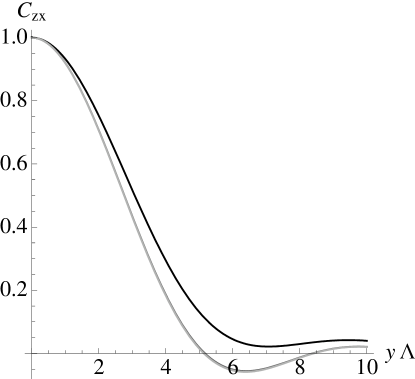
Refer to caption

Figure 3.4: Plot of the normalized correlation of the normal component of the stress tensor for different r𝑟r as a function of ΛyΛ𝑦\Lambda y. As before, the black line corresponds to r=1𝑟1r=1, dark gray corresponds to r=102𝑟superscript102r=10^{-2} and light gray corresponds to r=104𝑟superscript104r=10^{-4} (superposed).
3.4.4 Summing-up

Here we sum-up some important results obtained in this section. First, the three correlations normalized by it’s value at y=y𝑦superscript𝑦y=y^{\prime} share the following features:

  1. 1.

    the normalized correlation depends only weakly on the tension;

  2. 2.

    they present roughly a Gaussian behavior. Moreover, Cxxsubscript𝐶𝑥𝑥C_{xx} and Cyxsubscript𝐶𝑦𝑥C_{yx} are well approximated by

    Cxx(yy)Cxx(0)=Cyx(yy)Cyx(0)=eΛ2(yy)28,subscript𝐶𝑥𝑥𝑦superscript𝑦subscript𝐶𝑥𝑥0subscript𝐶𝑦𝑥𝑦superscript𝑦subscript𝐶𝑦𝑥0superscript𝑒superscriptΛ2superscript𝑦superscript𝑦28\frac{C_{xx}(y-y^{\prime})}{C_{xx}(0)}=\frac{C_{yx}(y-y^{\prime})}{C_{yx}(0)}=e^{-\frac{\Lambda^{2}(y-y^{\prime})^{2}}{8}}\,, (3.195)

    where Λ1=asuperscriptΛ1𝑎\Lambda^{-1}=a is the smallest wave-length cut-off;

  3. 3.

    the correlation is negligible for distances larger than 5a5𝑎5\,a, which is really small, considering a5nm𝑎5nma\approx 5\,\mathrm{nm}.

Finally, as the dependence on the tension happens mainly through the correlation at y=y𝑦superscript𝑦y=y^{\prime}, it is interesting to plot Cxx(0)subscript𝐶𝑥𝑥0C_{xx}(0), Cyx(0)subscript𝐶𝑦𝑥0C_{yx}(0) and Czx(0)subscript𝐶𝑧𝑥0C_{zx}(0), given in eq.(3.155), eq.(3.181) and eq.(3.194), respectively, as a function of the tension (see Fig. 3.5). Two important features of these curves will be reflected in the force fluctuation:

  1. 1.

    first, in the three cases, the dependence on the tension is not accentuated, implying that one could actually simply neglect from start every diagram proportional to σ2superscript𝜎2\sigma^{2} and σκ𝜎𝜅\sigma\kappa in the last sections;

  2. 2.

    secondly, the correlation of the component of the stress tensor normal to the membrane Czxsubscript𝐶𝑧𝑥C_{zx} is far bigger than the two other contributions, which are comparable among them.
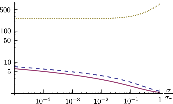
Refer to caption

Figure 3.5: Plot of Cxx(0)subscript𝐶𝑥𝑥0C_{xx}(0) (blue dashed line), Cyx(0)subscript𝐶𝑦𝑥0C_{yx}(0) (red solid line) and Czx(0)subscript𝐶𝑧𝑥0C_{zx}(0) (yellow dotted line) in units of σ0subscript𝜎0\sigma_{0} as a function of r=σ/σr𝑟𝜎subscript𝜎𝑟r=\sigma/\sigma_{r}. For the plot of Czx(0)subscript𝐶𝑧𝑥0C_{zx}(0), we have chosen 8πβκ=5008𝜋𝛽𝜅5008\pi\beta\kappa=500 as a typical value.

3.5 Fluctuation of the force

To obtain square of the force fluctuation in each direction, defined in eqs.(3.8)–(3.10), we must integrate the correlation function twice over the cut’s length:

(Δfx)2superscriptΔsubscript𝑓𝑥2\displaystyle(\Delta f_{x})^{2} =\displaystyle= L/2L/2Cxx(yy)𝑑y𝑑y,subscriptsuperscriptdouble-integral𝐿2𝐿2subscript𝐶𝑥𝑥𝑦superscript𝑦differential-d𝑦differential-dsuperscript𝑦\displaystyle\iint^{L/2}_{-L/2}C_{xx}(y-y^{\prime})\,dydy^{\prime}\,, (3.196)
(Δfy)2superscriptΔsubscript𝑓𝑦2\displaystyle(\Delta f_{y})^{2} =\displaystyle= L/2L/2Cyx(yy)𝑑y𝑑y,subscriptsuperscriptdouble-integral𝐿2𝐿2subscript𝐶𝑦𝑥𝑦superscript𝑦differential-d𝑦differential-dsuperscript𝑦\displaystyle\iint^{L/2}_{-L/2}C_{yx}(y-y^{\prime})\,dydy^{\prime}\,, (3.197)
(Δfz)2superscriptΔsubscript𝑓𝑧2\displaystyle(\Delta f_{z})^{2} =\displaystyle= L/2L/2Czx(yy)𝑑y𝑑y.subscriptsuperscriptdouble-integral𝐿2𝐿2subscript𝐶𝑧𝑥𝑦superscript𝑦differential-d𝑦differential-dsuperscript𝑦\displaystyle\iint^{L/2}_{-L/2}C_{zx}(y-y^{\prime})\,dydy^{\prime}\,. (3.198)

In the last section, we have seen that the correlations decrease very quickly, with a characteristic length of about =5a25nm5𝑎25nm\ell=5\,a\approx 25\,\mathrm{nm}. Recalling that L𝐿L is the length of the projected cut, it is reasonable thus to assume Lmuch-greater-than𝐿L\gg\ell. In Fig. 3.6, we can see a graphical representation of the integrals of eqs.(3.196)–(3.198) for the case where Lmuch-greater-than𝐿L\gg\ell.

Refer to caption

Figure 3.6: To obtain the square of the force fluctuation in each direction, one has to integrate the correlation function, here represented in purple, from L/2𝐿2-L/2 to L/2𝐿2L/2 at each point of the cut (domain shown by the blue dashed horizontal line and by the solid red line) and then sum all the contributions over the black line. As the correlation function decreases quickly compared to the length of the cut, remark that the final result would change only minimally if the colored lines where far lengthier.

In Fig. 3.6, we see that for Lmuch-greater-than𝐿L\gg\ell, eqs.(3.196)–(3.198) can be well approximated by

(Δfx)2superscriptΔsubscript𝑓𝑥2\displaystyle(\Delta f_{x})^{2} similar-to-or-equals\displaystyle\simeq LCxx(y)𝑑y,𝐿superscriptsubscriptsubscript𝐶𝑥𝑥𝑦differential-d𝑦\displaystyle L\,\int_{-\infty}^{\infty}C_{xx}(y)\,dy\,, (3.199)
(Δfy)2superscriptΔsubscript𝑓𝑦2\displaystyle(\Delta f_{y})^{2} similar-to-or-equals\displaystyle\simeq LCyx(y)𝑑y,𝐿superscriptsubscriptsubscript𝐶𝑦𝑥𝑦differential-d𝑦\displaystyle L\,\int_{-\infty}^{\infty}C_{yx}(y)\,dy\,, (3.200)
(Δfz)2superscriptΔsubscript𝑓𝑧2\displaystyle(\Delta f_{z})^{2} similar-to-or-equals\displaystyle\simeq LCzx(y)𝑑y.𝐿superscriptsubscriptsubscript𝐶𝑧𝑥𝑦differential-d𝑦\displaystyle L\,\int_{-\infty}^{\infty}C_{zx}(y)\,dy\,. (3.201)

For the two first cases, it is not possible to obtain an analytical equation from the exact expression of the correlation (eq.(3.149) and eq.(3.180)). We will thus use the Gaussian approximation given in eq.(3.195), yielding

(Δfx)2superscriptΔsubscript𝑓𝑥2\displaystyle(\Delta f_{x})^{2} similar-to-or-equals\displaystyle\simeq 8πLΛCxx(0)8𝜋𝐿Λsubscript𝐶𝑥𝑥0\displaystyle\sqrt{8\pi}\,\frac{L}{\Lambda}\,C_{xx}(0)
similar-to-or-equals\displaystyle\simeq 8πLΛ(σ022){3+[14r+3r2ln(1+1r)]ln(1+1r)},8𝜋𝐿Λsuperscriptsubscript𝜎0223delimited-[]14𝑟3superscript𝑟211𝑟11𝑟\displaystyle\sqrt{8\pi}\,\frac{L}{\Lambda}\,\left(\frac{\sigma_{0}^{2}}{2}\right)\left\{3+\left[1-4r+3r^{2}\ln\left(1+\frac{1}{r}\right)\right]\ln\left(1+\frac{1}{r}\right)\right\}\,,
(Δfy)2superscriptΔsubscript𝑓𝑦2\displaystyle(\Delta f_{y})^{2} similar-to-or-equals\displaystyle\simeq 8πLΛCyx(0)8𝜋𝐿Λsubscript𝐶𝑦𝑥0\displaystyle\sqrt{8\pi}\,\frac{L}{\Lambda}\,C_{yx}(0)
similar-to-or-equals\displaystyle\simeq 8πLΛ(σ022){1+[1+r2ln(1+1r)]ln(1+1r)},8𝜋𝐿Λsuperscriptsubscript𝜎0221delimited-[]1superscript𝑟211𝑟11𝑟\displaystyle\sqrt{8\pi}\,\frac{L}{\Lambda}\,\left(\frac{\sigma_{0}^{2}}{2}\right)\left\{1+\left[1+r^{2}\ln\left(1+\frac{1}{r}\right)\right]\ln\left(1+\frac{1}{r}\right)\right\}\,,
(Δfz)2superscriptΔsubscript𝑓𝑧2\displaystyle(\Delta f_{z})^{2} similar-to-or-equals\displaystyle\simeq 128πβκ3LΛ(σ022)(1+3r).128𝜋𝛽𝜅3𝐿Λsuperscriptsubscript𝜎02213𝑟\displaystyle\frac{128\pi\beta\kappa}{3}\,\frac{L}{\Lambda}\left(\frac{\sigma_{0}^{2}}{2}\right)\,(1+3r)\,. (3.204)

Not surprisingly, the dependence of the force fluctuation per unit length in terms of the tension shown in Fig. 3.7 is very similar to the trend shown in Fig. 3.5.
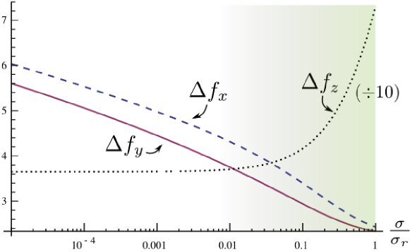
Refer to caption

Figure 3.7: Plot of ΔfxΔsubscript𝑓𝑥\Delta f_{x} (blue dashed line), ΔfyΔsubscript𝑓𝑦\Delta f_{y} (red solid line) and ΔfzΔsubscript𝑓𝑧\Delta f_{z} (black dotted line) in units of σ0L/Λsubscript𝜎0𝐿Λ\sigma_{0}\,\sqrt{L/\Lambda} as a function of r=σ/σr𝑟𝜎subscript𝜎𝑟r=\sigma/\sigma_{r}. In the plot of ΔfzΔsubscript𝑓𝑧\Delta f_{z}, we have chosen 8πβκ=5008𝜋𝛽𝜅5008\pi\beta\kappa=500 as a typical value. Note that the ΔfzΔsubscript𝑓𝑧\Delta f_{z} is much intenser – the yellow curve corresponds to the actual values divided by ten. The shaded green area indicates the region where the effects of stretching, which we have neglected, should be important.

Essentially, with Λ1=asuperscriptΛ1𝑎\Lambda^{-1}=a, we can say that

ΔfxΔfyLakBTaΔsubscript𝑓𝑥Δsubscript𝑓𝑦proportional-to𝐿𝑎subscript𝑘B𝑇𝑎\Delta f_{x}\approx\Delta f_{y}\propto\sqrt{\frac{L}{a}}\,\frac{k_{\mathrm{B}}T}{a}\, (3.205)

and

ΔfzLakBTκa2.proportional-toΔsubscript𝑓𝑧𝐿𝑎subscript𝑘B𝑇𝜅superscript𝑎2\Delta f_{z}\propto\sqrt{\frac{L}{a}}\,\sqrt{\frac{k_{\mathrm{B}}T\,\kappa}{a^{2}}}\,. (3.206)

In both cases, the dependence on L/a𝐿𝑎L/a can be understood by remembering that the correlations of the projected stress tensor decreases over a characteristic length of approximately 5a5𝑎5\,a for any component. For a cut of length L𝐿L, we have thus roughly L/a𝐿𝑎L/a uncorrelated patches of membrane, which with the Central Limit Theorem explains the factor L/a𝐿𝑎\sqrt{L/a}. Numerically, each patch contributes approximately kBT/a(4×1021)/(5×109)N1pNsimilar-tosubscript𝑘B𝑇𝑎4superscript10215superscript109Nsimilar-to1pNk_{\mathrm{B}}T/a\sim(4\times 10^{-21})/(5\times 10^{-9})\,\mathrm{N}\sim 1\,\mathrm{pN} for the transverse and parallel components of the force fluctuation and kBTκ/a2(4×1021×1019)/(5×109)2N4pNsimilar-tosubscript𝑘B𝑇𝜅superscript𝑎24superscript1021superscript1019superscript5superscript1092Nsimilar-to4pN\sqrt{k_{\mathrm{B}}T\,\kappa/a^{2}}\sim\sqrt{(4\times 10^{-21}\times 10^{-19})/(5\times 10^{-9})^{2}}\,\mathrm{N}\sim 4\,\mathrm{pN} for the normal component of the fluctuation.

A remarkable point is the fact that both the transverse ΔfxΔsubscript𝑓𝑥\Delta f_{x} and the parallel ΔfyΔsubscript𝑓𝑦\Delta f_{y} components of the fluctuation depend only on the temperature and on the microscopical cutoff a𝑎a, regardless of the rigidity or tension of the membrane.

3.6 In a nutshell

In this chapter, we have evaluated for the first time the fluctuation of the force exchanged through a cut of projected length L𝐿L in a planar membrane. To do so, we have introduced some diagrammatic tools useful in the following chapters. The calculation was done in two steps: first, we have evaluated the correlation of some elements of the projected stress tensor and after we have integrated them over the cut. These correlations present some interesting features: their shape do almost not depend on the tension and they decrease very quickly, becoming negligible for distances larger than 5a25nm5𝑎25nm5\,a\approx 25\,\mathrm{nm}, with a𝑎a of the order of the membrane thickness. For the fluctuation of the force component transverse to the cut, ΔfxΔsubscript𝑓𝑥\Delta f_{x}, and parallel to it, ΔfyΔsubscript𝑓𝑦\Delta f_{y}, we have obtained the same scaling behavior

ΔfxΔfyLakBTa,Δsubscript𝑓𝑥Δsubscript𝑓𝑦proportional-to𝐿𝑎subscript𝑘B𝑇𝑎\Delta f_{x}\approx\Delta f_{y}\propto\sqrt{\frac{L}{a}}\,\frac{k_{\mathrm{B}}T}{a}\,, (3.207)

whereas for the component perpendicular to the membrane, ΔfzΔsubscript𝑓𝑧\Delta f_{z}, we have obtained

ΔfzLakBTakBTκ.proportional-toΔsubscript𝑓𝑧𝐿𝑎subscript𝑘B𝑇𝑎subscript𝑘B𝑇𝜅\Delta f_{z}\propto\sqrt{\frac{L}{a}}\,\frac{k_{\mathrm{B}}T}{a}\,\sqrt{\frac{k_{\mathrm{B}}T}{\kappa}}\,. (3.208)

These equations hold up to a numerical factor of the order of the unity that depends very weakly on the tension. Interestingly, the scaling law for ΔfxΔsubscript𝑓𝑥\Delta f_{x} and ΔfyΔsubscript𝑓𝑦\Delta f_{y} depends neither on the bending rigidity.

Part II Vesicles

Chapter 4 Quasi-spherical vesicles

In chapter 1, we have seen that vesicles are widely used in experiments, since they are easy to assemble and to manipulate. Vesicles are used both in micropipette and adhesion experiments, in which one increases the mechanical tension τ𝜏\tau by flattening the membrane’s fluctuations and in contour analysis experiments, in which one measures r𝑟r, the large-scale counterpart of the tension σ𝜎\sigma, through the fluctuation spectrum. In the chapter 2, we have derived τ𝜏\tau as a function of σ𝜎\sigma for planar membranes, obtaining

τ=σσ0[1σσrln(1+σrσ)]𝜏𝜎subscript𝜎0delimited-[]1𝜎subscript𝜎𝑟1subscript𝜎𝑟𝜎\tau=\sigma-\sigma_{0}\left[1-\frac{\sigma}{\sigma_{r}}\ln\left(1+\frac{\sigma_{r}}{\sigma}\right)\right]\, (4.1)

in the limit of large membranes. In this equation, σr=κΛ2subscript𝜎𝑟𝜅superscriptΛ2\sigma_{r}=\kappa\Lambda^{2} is a tension of the order of the rupture tension, Λ=1/aΛ1𝑎\Lambda=1/a, where a𝑎a is a microscopical cut-off of the order of the membrane thickness and σ0=σr/(8πβκ)subscript𝜎0subscript𝜎𝑟8𝜋𝛽𝜅\sigma_{0}=\sigma_{r}/(8\pi\beta\kappa). This relation reduces simply to τσσ0similar-to-or-equals𝜏𝜎subscript𝜎0\tau\simeq\sigma-\sigma_{0} for membranes under small tensions (σ<102σr𝜎superscript102subscript𝜎𝑟\sigma<10^{-2}\,\sigma_{r}). We do not know, however, if eq.(4.1) still holds for vesicles since they have a different geometry and they present a supplementary volume constraint.

In this chapter, we shall thus calculate τ𝜏\tau from the projected stress tensor for the case of quasi-spherical vesicles. We shall examine both the usual case of a closed vesicle whose volume is constrained and the case of poked vesicles. We call poked vesicles those vesicles that are free to exchange liquid with the outer media. Experimentally, it can be achieved by embedding special proteins in the membrane or by making holes in it with a micropipette. They can however keep a pressure difference with the outer media if the inner/outer fluid contains molecules bigger than the holes, so they can not transit across the membrane.

In particular, we will address the following interesting questions, the first three having experimental implications while the last question deals with a more theoretical issue:

  1. 1.

    What is the difference between τ𝜏\tau for a quasi-spherical vesicle (closed or poked) and τ𝜏\tau for a planar membrane? Is there a characteristic radius over which they coincide, in which case one can simply consider the relation given in eq.(4.1)?

  2. 2.

    How does the volume constraint affect the expression for τ𝜏\tau?

  3. 3.

    Can τ𝜏\tau be negative, in which case the inner pressure of the vesicle would be smaller than the outer?

  4. 4.

    Can τ𝜏\tau be obtained by differentiating the free-energy with respect to the projected area? If so, what does projected area mean in the case of a vesicle?

Usually, as discussed in chapter 1, one should use the ADE-model Hamiltonian. We will however use the simpler Helfrich Hamiltonian, introduced in section 4.1. There, this choice will be justified. Following the same reasoning as in section 1.5.2, we derive the projected stress tensor for a quasi-spherical geometry in section 4.2. In section 4.3.1 we present some averages and correlations for the case of closed vesicles, which are used in section 4.3.2 to evaluate τclosedsubscript𝜏closed\tau_{\mathrm{closed}}. The results of the last two sections are easily transposed to the case of poked vesicles in section 4.4, where we obtain τpokedsubscript𝜏poked\tau_{\mathrm{poked}}.

Finally, we discuss the first three questions in section 4.5. We show that it is justified to use the relation given in eq.(4.1) for quasi-spherical vesicles, closed or poked, with a radius bigger than 1μm1𝜇m1\,\mathrm{\mu m}. Besides, the volume constraint seems to be unimportant for the dependence of τ𝜏\tau on σ𝜎\sigma. Experimentally, however, σ𝜎\sigma is not measurable. With vesicles, the true control parameter is the area excess, which depends considerably more on the volume constraint. We expect thus some difference between closed and poked vesicles, specially in the case of small vesicles. Lastly, we show that negative values of τ𝜏\tau are expected well before the transition to oblate shapes in both cases, implying that vesicles may support an internal pressure smaller than the outer.

At last, in section 4.6 we shall address the more theoretical question of recovering τ𝜏\tau for closed and poked vesicles by differentiating the free-energy. Differently for the case of planar membranes, the sense of the term projected area for a vesicle is not clear: it can refer to the area of a sphere with the average radius or the area of a sphere of volume V𝑉V, for instance. In this section, we shall see that indeed the term is not well-defined, since it corresponds to different area depending on whether the vesicle is closed or not.

All calculations and discussions presented here were done with the collaboration of Jean-Baptiste Fournier and Alberto Imparato. The main results can be found in ref. [5].

4.1 Parametrization and effective Hamiltonian

We consider a quasi-spherical vesicle whose area A𝐴A and volume V𝑉V are fixed (for closed vesicles). Its shape is parametrized by

𝒓=R[1+u(θ,ϕ)]𝒆r,𝒓𝑅delimited-[]1𝑢𝜃italic-ϕsubscript𝒆𝑟\bm{r}=R\left[1+u\left(\theta,\phi\right)\right]\,\bm{e}_{r}\,, (4.2)

where u1much-less-than𝑢1u\ll 1 (see Fig. 4.1). For closed vesicles, as in Seifert’s work [60], we choose the sphere of volume V𝑉V as the reference sphere, so that R=(34V/π)1/3𝑅superscript34𝑉𝜋13R=\left(\frac{3}{4}V/\pi\right)^{1/3}. Indeed, in experiments, one can control V𝑉V by lowering the ion concentration of the outer media of the vesicle, so it inflates at its maximum. Equivalently, using a micropipette, one can apply a large pressure difference through the membrane. In both cases, the excess area is negligible and thus from the optically resolvable shape, one deduces V𝑉V. In the case of poked vesicles, as there are no volume constraints, one cannot control V𝑉V. Instead, one can measure the average radius of the vesicle and deduce the average volume of the vesicle. In this case, we choose thus simply the average vesicle’s shape as the reference sphere, so that u(θ,ϕ)=0delimited-⟨⟩𝑢𝜃italic-ϕ0\langle u(\theta,\phi)\rangle=0.

Refer to caption
Figure 4.1: Parametrization in spherical coordinates of a vesicle (bold line) fluctuating around a reference sphere (dashed line). The inset shows the force exchanged through a cut that separates region 111 and region 222.

The area constraint reads

A=S𝑑A,𝐴subscript𝑆differential-d𝐴A=\int_{S}dA\,, (4.3)

with

dA=|θ𝒓×ϕ𝒓|dθdϕ,𝑑𝐴subscript𝜃𝒓subscriptitalic-ϕ𝒓𝑑𝜃𝑑italic-ϕdA=\left|\partial_{\theta}\bm{r}\times\partial_{\phi}\bm{r}\right|\,d\theta d\phi\,, (4.4)

where θ𝒓𝒓/θsubscript𝜃𝒓𝒓𝜃\partial_{\theta}\bm{r}\equiv\partial\bm{r}/\partial\theta, ϕ𝒓𝒓/ϕsubscriptitalic-ϕ𝒓𝒓italic-ϕ\partial_{\phi}\bm{r}\equiv\partial\bm{r}/\partial\phi, yielding, in terms of u𝑢u

A=R20π𝑑θ02π𝑑ϕ[1+u(θ,ϕ)][1+u(θ,ϕ)]2sin2θ+uϕ2+uθ2sin2θ.𝐴superscript𝑅2superscriptsubscript0𝜋differential-d𝜃superscriptsubscript02𝜋differential-ditalic-ϕdelimited-[]1𝑢𝜃italic-ϕsuperscriptdelimited-[]1𝑢𝜃italic-ϕ2superscript2𝜃superscriptsubscript𝑢italic-ϕ2superscriptsubscript𝑢𝜃2superscript2𝜃A=R^{2}\int_{0}^{\pi}d\theta\int_{0}^{2\pi}d\phi\,[1+u(\theta,\phi)]\sqrt{\left[1+u(\theta,\phi)\right]^{2}\sin^{2}\theta+u_{\phi}^{2}+u_{\theta}^{2}\sin^{2}\theta}\,. (4.5)

Here and throughout this section, uiu/isubscript𝑢𝑖𝑢𝑖u_{i}\equiv\partial u/\partial i, uij2u/ijsubscript𝑢𝑖𝑗superscript2𝑢𝑖𝑗u_{ij}\equiv\partial^{2}u/\partial i\partial j, where i,j{θ,ϕ}𝑖𝑗𝜃italic-ϕi,j\in\{\theta,\phi\}. Latin indices will denote either θ𝜃\theta or ϕitalic-ϕ\phi, not r𝑟r. The volume constraint, important for closed vesicles, reads

V=13R30π𝑑θ02π𝑑ϕ[1+u(θ,ϕ)]3sinθ.𝑉13superscript𝑅3superscriptsubscript0𝜋differential-d𝜃superscriptsubscript02𝜋differential-ditalic-ϕsuperscriptdelimited-[]1𝑢𝜃italic-ϕ3𝜃V=\frac{1}{3}R^{3}\int_{0}^{\pi}d\theta\int_{0}^{2\pi}d\phi\,[1+u(\theta,\phi)]^{3}\sin\theta\,. (4.6)

As we have seen in section 1.3, the energy of a vesicle is best described by the area-difference elasticity (ADE𝐴𝐷𝐸ADE) model. Seifert [60] has however shown that in the quasi-spherical limit, the ADE𝐴𝐷𝐸ADE Hamiltonian was equivalent to the minimal Helfrich model, i. e., the spontaneous curvature (SC𝑆𝐶SC) model with vanishing spontaneous curvature. Hence, we adopt the latter, which corresponds to an effective Hamiltonian

=S2κH2𝑑A,subscript𝑆2𝜅superscript𝐻2differential-d𝐴\mathcal{H}=\int_{S}2\kappa H^{2}\,dA\,, (4.7)

supplemented by the area and (if necessary) volume constraints given in eqs.(4.5)–(4.6). While the volume constraint is quite easy to implement, it is difficult to handle the surface constraint exactly [60]. We shall therefore use the traditional approach, namely introducing a Lagrange multiplier σ𝜎\sigma playing the role of a tension in order to take into account the area constraint. Again, as discussed by Seifert [60], this approach gives correct results in the small excess area limit, in which we shall place ourselves in the following. The effective Hamiltonian thus reads

=S(2κH2+σ)𝑑A,subscript𝑆2𝜅superscript𝐻2𝜎differential-d𝐴\mathcal{H}=\int_{S}\left(2\kappa H^{2}+\sigma\right)\,dA\,, (4.8)

with the additional constraint given by eq.(4.6) for closed vesicles.

From differential geometry, dA𝑑𝐴dA is given by eq.(4.4) and

H=2bBcAaCACB2,𝐻2𝑏𝐵𝑐𝐴𝑎𝐶𝐴𝐶superscript𝐵2H=\frac{2bB-cA-aC}{AC-B^{2}}\,, (4.9)

with A=(θ𝒓)2𝐴superscriptsubscript𝜃𝒓2A=(\partial_{\theta}\bm{r})^{2}, B=(θ𝒓)(ϕ𝒓)𝐵subscript𝜃𝒓subscriptitalic-ϕ𝒓B=(\partial_{\theta}\bm{r})\cdot(\partial_{\phi}\bm{r}), C=(ϕ𝒓)2𝐶superscriptsubscriptitalic-ϕ𝒓2C=(\partial_{\phi}\bm{r})^{2}, a=𝒏θ2𝒓𝑎𝒏superscriptsubscript𝜃2𝒓a=\bm{n}\cdot\partial_{\theta}^{2}\bm{r}, b=𝒏θϕ𝒓𝑏𝒏subscript𝜃subscriptitalic-ϕ𝒓b=\bm{n}\cdot\partial_{\theta}\partial_{\phi}\bm{r}, c=𝒏ϕ2𝒓𝑐𝒏superscriptsubscriptitalic-ϕ2𝒓c=\bm{n}\cdot\partial_{\phi}^{2}\bm{r}, 𝒏=(θ𝒓×ϕ𝒓)/|θ𝒓×ϕ𝒓|𝒏subscript𝜃𝒓subscriptitalic-ϕ𝒓subscript𝜃𝒓subscriptitalic-ϕ𝒓\bm{n}=(\partial_{\theta}\bm{r}\times\partial_{\phi}\bm{r})/|\partial_{\theta}\bm{r}\times\partial_{\phi}\bm{r}| being the normal to the surface. Up to the second order on u(θ,ϕ)𝑢𝜃italic-ϕu(\theta,\phi), we have thus

=Sh(u,{ui},{uij})𝑑θ𝑑ϕ,subscript𝑆𝑢subscript𝑢𝑖subscript𝑢𝑖𝑗differential-d𝜃differential-ditalic-ϕ\mathcal{H}=\int_{S}h\left(u,\{u_{i}\},\{u_{ij}\}\right)\,d\theta d\phi\,, (4.10)

with [110] [111]

h\displaystyle h =\displaystyle= (2κ+R2σ)sinθ2𝜅superscript𝑅2𝜎𝜃\displaystyle(2\kappa+R^{2}\sigma)\sin\theta (4.11)
+\displaystyle+ 2sinθ[R2σuκ(uϕϕcsc2θ+uθcotθ+uθθ)]2𝜃delimited-[]superscript𝑅2𝜎𝑢𝜅subscript𝑢italic-ϕitalic-ϕsuperscript2𝜃subscript𝑢𝜃𝜃subscript𝑢𝜃𝜃\displaystyle 2\sin\theta\left[R^{2}\sigma u-\kappa\left({u_{\phi\phi}\csc^{2}\theta+u_{\theta}\cot\theta+u_{\theta\theta}}\right)\right]
+\displaystyle+ 12sinθ[2R2σu2+(2κ+R2σ)(uθ2+uϕ2csc2θ)\displaystyle\frac{1}{2}\sin\theta\left[2R^{2}\sigma u^{2}+(2\kappa+R^{2}\sigma)(u_{\theta}^{2}+u_{\phi}^{2}\csc^{2}\theta)\right.
+\displaystyle+ κ(uθcotθ+uϕϕcsc2θ)2+κuθθ(uθθ+4u)𝜅superscriptsubscript𝑢𝜃𝜃subscript𝑢italic-ϕitalic-ϕsuperscript2𝜃2𝜅subscript𝑢𝜃𝜃subscript𝑢𝜃𝜃4𝑢\displaystyle\kappa\left({u_{\theta}\cot\theta+u_{\phi\phi}\csc^{2}\theta}\right)^{2}+\kappa\,u_{\theta\theta}\,(u_{\theta\theta}+4u)
+\displaystyle+ 2κ(uθθ+2u)(uθcotθ+uϕϕcsc2θ)]+𝒪(u3).\displaystyle\left.2\kappa\,(u_{\theta\theta}+2u)\left({u_{\theta}\cot\theta+u_{\phi\phi}\csc^{2}\theta}\right)\right]+\mathcal{O}(u^{3})\,.

4.2 Derivation of the stress tensor for a quasi-spherical geometry

Let us consider an infinitesimal cut at constant longitude (ϕitalic-ϕ\phi constant) separating a region 111 from a region 222 (see Fig. 4.1). The normal to the projection of this cut onto the reference sphere is 𝒎=𝒆ϕ𝒎subscript𝒆italic-ϕ\bm{m}=\bm{e}_{\phi}. Analogously to the case of planar membranes presented in section 1.5.2, the projected stress tensor 𝚺𝚺\bm{\Sigma} in spherical geometry relates by definition linearly the force d𝑭𝑑𝑭d\bm{F} that region 111 exerts on region 222 to the angular length ds=dθ𝑑𝑠𝑑𝜃ds=d\theta of the projection of the cut onto the reference sphere:

d𝑭𝑑𝑭\displaystyle d\bm{F} =\displaystyle= 𝚺𝒎ds,𝚺𝒎𝑑𝑠\displaystyle\bm{\Sigma}\cdot\bm{m}\,ds\,, (4.12)
=\displaystyle= (Σθϕ𝒆θ+Σϕϕ𝒆ϕ+Σrϕ𝒆r)dθ.subscriptΣ𝜃italic-ϕsubscript𝒆𝜃subscriptΣitalic-ϕitalic-ϕsubscript𝒆italic-ϕsubscriptΣ𝑟italic-ϕsubscript𝒆𝑟𝑑𝜃\displaystyle\left(\Sigma_{\theta\phi}\,\bm{e}_{\theta}+\Sigma_{\phi\phi}\,\bm{e}_{\phi}+\Sigma_{r\phi}\,\bm{e}_{r}\right)\,d\theta\,.

Likewise, for a cut at constant latitude (θ𝜃\theta constant), with 𝒎=𝒆θ𝒎subscript𝒆𝜃\bm{m}=\bm{e}_{\theta} and ds=dϕ𝑑𝑠𝑑italic-ϕds=d\phi, we have

d𝑭𝑑𝑭\displaystyle d\bm{F} =\displaystyle= 𝚺𝒎dϕ,𝚺𝒎𝑑italic-ϕ\displaystyle\bm{\Sigma}\cdot\bm{m}\,d\phi\,, (4.13)
=\displaystyle= (Σθθ𝒆θ+Σϕθ𝒆ϕ+Σrθ𝒆r)dϕ.subscriptΣ𝜃𝜃subscript𝒆𝜃subscriptΣitalic-ϕ𝜃subscript𝒆italic-ϕsubscriptΣ𝑟𝜃subscript𝒆𝑟𝑑italic-ϕ\displaystyle\left(\Sigma_{\theta\theta}\,\bm{e}_{\theta}+\Sigma_{\phi\theta}\,\bm{e}_{\phi}+\Sigma_{r\theta}\,\bm{e}_{r}\right)\,d\phi\,.

For an oblique cut, d𝑭𝑑𝑭d\bm{F} is obtained by decomposing 𝒎𝒎\bm{m} along 𝒆θsubscript𝒆𝜃\bm{e}_{\theta} and 𝒆ϕsubscript𝒆italic-ϕ\bm{e}_{\phi}.

The derivation of the projected stress tensor in spherical geometry follows the same route as for planar geometry (section 1.5.2). We consider a patch of membrane delimited by a closed curve, corresponding to a domain ΩΩ\Omega on the reference sphere enclosed by the curve ΩΩ\partial\Omega. The membrane within the patch is assumed to be deformed, at equilibrium, by means of a distribution of surface and boundary forces (and a distribution of boundary torques). To each point of this patch, we impose an arbitrary displacement δ𝒂=δar𝒆r+δaθ𝒆θ+δaϕ𝒆ϕ𝛿𝒂𝛿subscript𝑎𝑟subscript𝒆𝑟𝛿subscript𝑎𝜃subscript𝒆𝜃𝛿subscript𝑎italic-ϕsubscript𝒆italic-ϕ\delta\bm{a}=\delta a_{r}\,\bm{e}_{r}+\delta a_{\theta}\,\bm{e}_{\theta}+\delta a_{\phi}\,\bm{e}_{\phi} that keeps the orientation of the membrane’s normal 𝒏𝒏\bm{n} constant along the boundary, so that the torques produce no work (see Fig. 4.2).
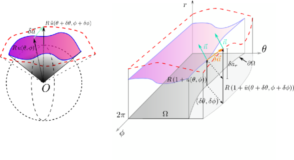
Refer to caption
Figure 4.2: On the left we see a patch of quasi-spherical membrane before (shaded shape) and after (dashed red shape) the displacement δ𝒂𝛿𝒂\delta\bm{a}. At right, we show the same displacement in the (θ,ϕ,r)𝜃italic-ϕ𝑟(\theta,\phi,r) space. From this drawing, it is easier to see the relation between δ𝒂𝛿𝒂\delta\bm{a}, δu𝛿𝑢\delta u, δθ𝛿𝜃\delta\theta and δϕ𝛿italic-ϕ\delta\phi.

On the one hand, the boundary energy variation, after integration by parts, reads

δ=Ωmi[hδi+(huiihuij)δu+huijδuj]𝑑s,𝛿subscriptΩsubscript𝑚𝑖delimited-[]𝛿𝑖subscript𝑢𝑖subscript𝑖subscript𝑢𝑖𝑗𝛿𝑢subscript𝑢𝑖𝑗𝛿subscript𝑢𝑗differential-d𝑠\delta\mathcal{H}=\int_{\partial\Omega}m_{i}\left[h\,\delta i+\left(\frac{\partial h}{\partial u_{i}}-\partial_{i}\frac{\partial h}{\partial u_{ij}}\right)\delta u+\frac{\partial h}{\partial u_{ij}}\,\delta u_{j}\right]\,ds\,, (4.14)

where ds𝑑𝑠ds is the arc-length in the (θ,ϕ)𝜃italic-ϕ(\theta,\phi) space, hh is given by eq.(4.11), 𝒎𝒎\bm{m} is the normal to ΩΩ\partial\Omega, and δi{δθ,δϕ}𝛿𝑖𝛿𝜃𝛿italic-ϕ\delta i\in\{\delta\theta,\delta\phi\} corresponds to the variation of ΩΩ\partial\Omega. On the other hand, the work of the force exerted through the boundary reads

δ=Ωδ𝒂𝚺𝒎𝑑s.𝛿subscriptΩ𝛿𝒂𝚺𝒎differential-d𝑠\delta\mathcal{H}=\int_{\partial\Omega}\delta\bm{a}\cdot\bm{\Sigma}\cdot\,\bm{m}\,ds\,. (4.15)

By comparing eqs.(4.14) and (4.15), one can obtain 𝚺𝚺\bm{\Sigma}. Accordingly, one has to derive δθ𝛿𝜃\delta\theta, δϕ𝛿italic-ϕ\delta\phi, δu𝛿𝑢\delta u, δuθ𝛿subscript𝑢𝜃\delta u_{\theta} and δuϕ𝛿subscript𝑢italic-ϕ\delta u_{\phi} in terms of δ𝒂𝛿𝒂\delta\bm{a}. The first three can be obtained by identifying the new membrane’s shape u~=u+δu~𝑢𝑢𝛿𝑢\tilde{u}=u+\delta u with the translation of the old one: R[1+u~(θ+δθ,ϕ+δϕ)]𝒆r(θ+δθ,ϕ+δϕ)=R[1+u(θ,ϕ)]𝒆r+δ𝒂𝑅delimited-[]1~𝑢𝜃𝛿𝜃italic-ϕ𝛿italic-ϕsubscript𝒆𝑟𝜃𝛿𝜃italic-ϕ𝛿italic-ϕ𝑅delimited-[]1𝑢𝜃italic-ϕsubscript𝒆𝑟𝛿𝒂R[1+\tilde{u}(\theta+\delta\theta,\phi+\delta\phi)]\,\bm{e}_{r}(\theta+\delta\theta,\phi+\delta\phi)=R[1+u(\theta,\phi)]\,\bm{e}_{r}+\delta\bm{a} (see Fig. 4.2). This leads to

δar𝛿subscript𝑎𝑟\displaystyle\delta a_{r} =\displaystyle= R(uθδθ+uϕδϕ+δu),𝑅subscript𝑢𝜃𝛿𝜃subscript𝑢italic-ϕ𝛿italic-ϕ𝛿𝑢\displaystyle R\,(u_{\theta}\,\delta\theta+u_{\phi}\,\delta\phi+\delta u)\,, (4.16)
δaθ𝛿subscript𝑎𝜃\displaystyle\delta a_{\theta} =\displaystyle= R(1+u)δθ,𝑅1𝑢𝛿𝜃\displaystyle R\,(1+u)\,\delta\theta\,, (4.17)
δaϕ𝛿subscript𝑎italic-ϕ\displaystyle\delta a_{\phi} =\displaystyle= R(1+u)sinθδϕ.𝑅1𝑢𝜃𝛿italic-ϕ\displaystyle R\,(1+u)\sin\theta\,\delta\phi\,. (4.18)

Let δ𝒏=𝒏~(θ+δθ,ϕ+δϕ)𝒏(θ,ϕ)𝛿𝒏~𝒏𝜃𝛿𝜃italic-ϕ𝛿italic-ϕ𝒏𝜃italic-ϕ\delta\bm{n}=\tilde{\bm{n}}(\theta+\delta\theta,\phi+\delta\phi)-\bm{n}(\theta,\phi) be the variation of the normal, where 𝒏~~𝒏\tilde{\bm{n}} is the normal to the shape defined by u~(θ,ϕ)~𝑢𝜃italic-ϕ\tilde{u}(\theta,\phi) and 𝒏=𝒕θ×𝒕ϕ/|𝒕θ×𝒕ϕ|𝒏subscript𝒕𝜃subscript𝒕italic-ϕsubscript𝒕𝜃subscript𝒕italic-ϕ\bm{n}=\bm{t}_{\theta}\times\bm{t}_{\phi}/|\bm{t}_{\theta}\times\bm{t}_{\phi}|, with 𝒕i=i𝒓subscript𝒕𝑖subscript𝑖𝒓\bm{t}_{i}=\partial_{i}\bm{r}. The variation of the normal vanishes (implying no work of the torques) if δ𝒏𝒕θ=0𝛿𝒏subscript𝒕𝜃0\delta\bm{n}\cdot\bm{t}_{\theta}=0 and δ𝒏𝒕ϕ=0𝛿𝒏subscript𝒕italic-ϕ0\delta\bm{n}\cdot\bm{t}_{\phi}=0 over the border, yielding

δuθ𝛿subscript𝑢𝜃\displaystyle\delta u_{\theta} =\displaystyle= 11+u{δθ[(1+u)2+2uθ2(1+u)uθθ]\displaystyle\frac{1}{1+u}\Big{\{}\delta\theta\left[(1+u)^{2}+2u_{\theta}^{2}-(1+u)\,u_{\theta\theta}\right]\phantom{\frac{\delta}{\delta}}
+\displaystyle+ δϕsinθ[(1+u)uϕcosθ(1+u)uθϕsinθ\displaystyle\frac{\delta\phi}{\sin\theta}\left[(1+u)\,u_{\phi}\cos\theta-(1+u)\,u_{\theta\phi}\sin\theta\right.
+\displaystyle+ 2uϕuθsinθ]+δuuθ},\displaystyle\left.2u_{\phi}u_{\theta}\sin\theta\right]+\delta u\,u_{\theta}\Big{\}}\,,
(4.19)
δuϕ𝛿subscript𝑢italic-ϕ\displaystyle\delta u_{\phi} =\displaystyle= 11+u{δθ[(1+u)uϕcotθ+2uθuϕ\displaystyle\frac{1}{1+u}\Big{\{}\delta\theta\left[(1+u)\,u_{\phi}\cot\theta+2u_{\theta}u_{\phi}\right. (4.20)
\displaystyle- (1+u)uθϕ]+δϕ[(1+u)2sin2θ+2uϕ2\displaystyle\left.(1+u)\,u_{\theta\phi}\right]+\delta\phi\left[(1+u)^{2}\sin^{2}\theta+2u_{\phi}^{2}\right.
\displaystyle- (1+u)(uθcosθsinθ+uϕϕ)]+δuuϕ}.\displaystyle\left.(1+u)(u_{\theta}\cos\theta\sin\theta+u_{\phi\phi})\right]+\delta u\,u_{\phi}\Big{\}}\,.

These equations, combined with eqs.(4.16)-(4.18), allow us to write δuθ𝛿subscript𝑢𝜃\delta u_{\theta} and δuϕ𝛿subscript𝑢italic-ϕ\delta u_{\phi} in terms of δ𝒂𝛿𝒂\delta\bm{a}. Up to order u2superscript𝑢2u^{2}, we obtain

δθ𝛿𝜃\displaystyle\delta\theta =\displaystyle= δaθR(1u+u2),𝛿subscript𝑎𝜃𝑅1𝑢superscript𝑢2\displaystyle\frac{\delta a_{\theta}}{R}(1-u+u^{2})\,, (4.21)
δϕ𝛿italic-ϕ\displaystyle\delta\phi =\displaystyle= δaϕRsinθ(1u+u2),𝛿subscript𝑎italic-ϕ𝑅𝜃1𝑢superscript𝑢2\displaystyle\frac{\delta a_{\phi}}{R\sin\theta}(1-u+u^{2})\,, (4.22)
δu𝛿𝑢\displaystyle\delta u =\displaystyle= 1R[δar(1u)(δaϕuϕcscθ+δaθuθ)],1𝑅delimited-[]𝛿subscript𝑎𝑟1𝑢𝛿subscript𝑎italic-ϕsubscript𝑢italic-ϕ𝜃𝛿subscript𝑎𝜃subscript𝑢𝜃\displaystyle\frac{1}{R}\left[\delta a_{r}-(1-u)\,(\delta a_{\phi}u_{\phi}\csc\theta+\delta a_{\theta}u_{\theta})\right]\,, (4.23)
δuθ𝛿subscript𝑢𝜃\displaystyle\delta u_{\theta} =\displaystyle= 1R{δar(1u)uθ+δaθ[1+uθ2(1u)uθθ]\displaystyle\frac{1}{R}\Big{\{}\delta a_{r}\,(1-u)\,u_{\theta}+\delta a_{\theta}\left[1+u_{\theta}^{2}-(1-u)\,u_{\theta\theta}\right]
+\displaystyle+ δaϕcscθ[uϕ[(1u)cotθ+uθ](1u)uθϕ]},\displaystyle\delta a_{\phi}\csc\theta\big{[}u_{\phi}[(1-u)\cot\theta+u_{\theta}]-(1-u)\,u_{\theta\phi}\big{]}\Big{\}}\,,
(4.24)
δuϕ𝛿subscript𝑢italic-ϕ\displaystyle\delta u_{\phi} =\displaystyle= 1R{δaθ[uϕ[(1u)cotθ+uθ](1u)uθϕ]\displaystyle\frac{1}{R}\Big{\{}\delta a_{\theta}\big{[}u_{\phi}\,[(1-u)\,\cot\theta+u_{\theta}]-(1-u)\,u_{\theta\phi}\big{]} (4.25)
+\displaystyle+ δar(1u)uϕ+δaϕcscθ[sin2θ+uϕ2\displaystyle\delta a_{r}\,(1-u)\,u_{\phi}+\delta a_{\phi}\csc\theta\big{[}\sin^{2}\theta+u_{\phi}^{2}
\displaystyle- (1u)(uϕϕ+uθcosθsinθ)]}.\displaystyle(1-u)\,(u_{\phi\phi}+u_{\theta}\cos\theta\sin\theta)\big{]}\Big{\}}\,.

These expressions are to be inserted into eq.(4.14). Note that it is necessary to expand hh up to 𝒪(u3)𝒪superscript𝑢3\mathcal{O}(u^{3}) in order to obtain h/uisubscript𝑢𝑖\partial h/\partial u_{i} and h/uijsubscript𝑢𝑖𝑗\partial h/\partial u_{ij} consistently at 𝒪(u2)𝒪superscript𝑢2\mathcal{O}(u^{2}) in eq.(4.14). This means adding

h3subscript3\displaystyle h_{3} =\displaystyle= κsinθ{4csc4θuϕuθuθϕ+2uθ2uθθ\displaystyle-\kappa\sin\theta\,\big{\{}4\csc^{4}\theta\,u_{\phi}\,u_{\theta}\,u_{\theta\phi}+2u_{\theta}^{2}\,u_{\theta\theta} (4.26)
\displaystyle- 2uϕ2csc2θ(uϕϕcsc2θuθcotθ)2superscriptsubscript𝑢italic-ϕ2superscript2𝜃subscript𝑢italic-ϕitalic-ϕsuperscript2𝜃subscript𝑢𝜃𝜃\displaystyle 2u_{\phi}^{2}\,\csc^{2}\theta\,\big{(}u_{\phi\phi}\,\csc^{2}\theta-u_{\theta}\,\cot\theta\big{)}
+\displaystyle+ u[uθθ2+uθ2(2+cot2θ)+2uϕ2csc2θ+uϕϕ2csc4θ\displaystyle u\left[u_{\theta\theta}^{2}+u_{\theta}^{2}\,\left(2+\cot^{2}\theta\right)+2\,u_{\phi}^{2}\,\csc^{2}\theta+u_{\phi\phi}^{2}\,\csc^{4}\theta\right.
+\displaystyle+ 2uθuθθcotθ+2uθuϕϕcsc2θcotθ+2uθθuϕϕcsc2θ]\displaystyle\left.2\,u_{\theta}\,u_{\theta\theta}\,\cot\theta+2\,u_{\theta}\,u_{\phi\phi}\,\csc^{2}\theta\cot\theta+2\,u_{\theta\theta}\,u_{\phi\phi}\csc^{2}\theta\right]
+\displaystyle+ 2u2(uθθ+uθcotθ+uϕϕcsc2θ)}\displaystyle 2u^{2}\left(u_{\theta\theta}+u_{\theta}\cot\theta+u_{\phi\phi}\csc^{2}\theta\right)\big{\}}

to eq.(4.11) before calculating the derivatives. Finally, comparing eq.(4.14) and eq.(4.15), we obtain

ΣθθsubscriptΣ𝜃𝜃\displaystyle\Sigma_{\theta\theta} =\displaystyle= 12R{R2σsinθ(2+2u+uϕ2csc2θuθ2)\displaystyle\frac{1}{2R}\Big{\{}R^{2}\sigma\sin\theta\left(2+2u+u_{\phi}^{2}\csc^{2}\theta-u_{\theta}^{2}\right)
+κ[uϕϕ2csc3θuθθ2sinθ+2uθ(uθϕϕcscθ+uθθθsinθ)]𝜅delimited-[]superscriptsubscript𝑢italic-ϕitalic-ϕ2superscript3𝜃superscriptsubscript𝑢𝜃𝜃2𝜃2subscript𝑢𝜃subscript𝑢𝜃italic-ϕitalic-ϕ𝜃subscript𝑢𝜃𝜃𝜃𝜃\displaystyle+\kappa\left[{u_{\phi\phi}^{2}\,\csc^{3}\theta-u_{\theta\theta}^{2}\,\sin\theta+2u_{\theta}\,\left(u_{\theta\phi\phi}\,\csc\theta+u_{\theta\theta\theta}\,\sin\theta\right)}\right]
+κcscθ[2uϕ2uθ2cos2θ2uϕϕ(1+uθcotθ)+4u(uϕϕuθθsin2θ)]𝜅𝜃delimited-[]2superscriptsubscript𝑢italic-ϕ2superscriptsubscript𝑢𝜃2superscript2𝜃2subscript𝑢italic-ϕitalic-ϕ1subscript𝑢𝜃𝜃4𝑢subscript𝑢italic-ϕitalic-ϕsubscript𝑢𝜃𝜃superscript2𝜃\displaystyle+\kappa\,\csc\theta\left[{2u_{\phi}^{2}-u_{\theta}^{2}\,\cos^{2}\theta-2u_{\phi\phi}\,(1+u_{\theta}\,\cot\theta)+4u\,\left(u_{\phi\phi}-u_{\theta\theta}\,\sin^{2}\theta\right)}\right]
+2κ[uθθ(sinθ+uθcosθ)+(2u1)uθcosθ]},\displaystyle+2\kappa\big{[}u_{\theta\theta}\,(\sin\theta+u_{\theta}\cos\theta)+(2u-1)\,u_{\theta}\,\cos\theta\big{]}\Big{\}}\,,
ΣϕθsubscriptΣitalic-ϕ𝜃\displaystyle\Sigma_{\phi\theta} =\displaystyle= Rσuθuϕ+κR(2uθϕuϕcotθ)+κR(4uuϕcotθuϕuϕϕcotθcsc2θ\displaystyle-R\sigma u_{\theta}u_{\phi}+\frac{\kappa}{R}\left(2u_{\theta\phi}-u_{\phi}\cot\theta\right)+\frac{\kappa}{R}\Big{(}4u\,u_{\phi}\,\cot\theta-u_{\phi}\,u_{\phi\phi}\,\cot\theta\csc^{2}\theta (4.28)
+\displaystyle+ uθuϕ4uuθϕuϕϕuθϕcsc2θuθuθϕcotθ+uϕuθϕϕcsc2θsubscript𝑢𝜃subscript𝑢italic-ϕ4𝑢subscript𝑢𝜃italic-ϕsubscript𝑢italic-ϕitalic-ϕsubscript𝑢𝜃italic-ϕsuperscript2𝜃subscript𝑢𝜃subscript𝑢𝜃italic-ϕ𝜃subscript𝑢italic-ϕsubscript𝑢𝜃italic-ϕitalic-ϕsuperscript2𝜃\displaystyle u_{\theta}u_{\phi}-4u\,u_{\theta\phi}-u_{\phi\phi}\,u_{\theta\phi}\,\csc^{2}\theta-u_{\theta}\,u_{\theta\phi}\,\cot\theta+u_{\phi}\,u_{\theta\phi\phi}\,\csc^{2}\theta
+\displaystyle+ 2uϕuθθcotθuθϕuθθ+uϕuθθθ),\displaystyle 2u_{\phi}\,u_{\theta\theta}\,\cot\theta-u_{\theta\phi}\,u_{\theta\theta}+u_{\phi}\,u_{\theta\theta\theta}\Big{)}\,,
ΣrθsubscriptΣ𝑟𝜃\displaystyle\Sigma_{r\theta} =\displaystyle= RσsinθuθκR[(12u)uθ(2sinθcscθ)+uθθcosθ2uϕϕcotθcscθ\displaystyle R\sigma\sin\theta\,u_{\theta}-\frac{\kappa}{R}\Big{[}\left(1-2u\right)\,u_{\theta}\,\left(2\sin\theta-\csc\theta\right)+u_{\theta\theta}\,\cos\theta-2u_{\phi\phi}\,\cot\theta\csc\theta
+\displaystyle+ uθϕϕcscθ+uθθθsinθ]κR[2uϕ2cotθcscθuθ2cosθ+4uuϕϕcotθcscθ\displaystyle u_{\theta\phi\phi}\,\csc\theta+u_{\theta\theta\theta}\,\sin\theta\Big{]}-\frac{\kappa}{R}\Big{[}2u_{\phi}^{2}\,\cot\theta\csc\theta-u_{\theta}^{2}\,\cos\theta+4u\,u_{\phi\phi}\,\cot\theta\csc\theta
\displaystyle- 2uuθθcosθ2uuθϕϕcscθ2uuθθθsinθ+uϕϕuθcscθ3uθuθθsinθ],\displaystyle 2u\,u_{\theta\theta}\cos\theta-2u\,u_{\theta\phi\phi}\csc\theta-2u\,u_{\theta\theta\theta}\sin\theta+u_{\phi\phi}\,u_{\theta}\csc\theta-3u_{\theta}\,u_{\theta\theta}\sin\theta\Big{]}\,,
ΣϕϕsubscriptΣitalic-ϕitalic-ϕ\displaystyle\Sigma_{\phi\phi} =\displaystyle= 12R{R2σ(2+2uuϕ2csc2θ+uθ2)\displaystyle\frac{1}{2R}\Big{\{}R^{2}\sigma\big{(}2+2u-u_{\phi}^{2}\csc^{2}\theta+u_{\theta}^{2}\big{)}
+\displaystyle+ κ[uϕϕ2csc4θ+uθθ2+2uϕcsc2θ(uϕϕϕcsc2θ+uθθϕ)]𝜅delimited-[]superscriptsubscript𝑢italic-ϕitalic-ϕ2superscript4𝜃superscriptsubscript𝑢𝜃𝜃22subscript𝑢italic-ϕsuperscript2𝜃subscript𝑢italic-ϕitalic-ϕitalic-ϕsuperscript2𝜃subscript𝑢𝜃𝜃italic-ϕ\displaystyle\kappa\big{[}-u_{\phi\phi}^{2}\csc^{4}\theta+u_{\theta\theta}^{2}+2u_{\phi}\csc^{2}\theta\big{(}u_{\phi\phi\phi}\csc^{2}\theta+u_{\theta\theta\phi}\big{)}\big{]}
+\displaystyle+ κcsc2θ[2uϕ2+uθ2(3sin2θ1)+2uϕϕ(1uθcotθ2u)]𝜅superscript2𝜃delimited-[]2superscriptsubscript𝑢italic-ϕ2superscriptsubscript𝑢𝜃23superscript2𝜃12subscript𝑢italic-ϕitalic-ϕ1subscript𝑢𝜃𝜃2𝑢\displaystyle\kappa\csc^{2}\theta\left[{2u_{\phi}^{2}+u_{\theta}^{2}\,\left(3\sin^{2}\theta-1\right)+2u_{\phi\phi}\left(1-u_{\theta}\cot\theta-2u\right)}\right]
+\displaystyle+ 2κ(12u)uθcotθ2κ(12u)uθθ+2κuϕuθϕcsc2θcotθ},\displaystyle 2\kappa(1-2u)u_{\theta}\cot\theta-2\kappa(1-2u)u_{\theta\theta}+2\kappa u_{\phi}\,u_{\theta\phi}\csc^{2}\theta\cot\theta\Big{\}}\,,
ΣθϕsubscriptΣ𝜃italic-ϕ\displaystyle\Sigma_{\theta\phi} =\displaystyle= Rσcscθuθuϕ+κcscθR[(uϕcotθuθϕ)(2+4u+uθθ+uϕϕcsc2θ)\displaystyle-R\sigma\csc\theta\,u_{\theta}u_{\phi}+\frac{\kappa\csc\theta}{R}\Big{[}\left(u_{\phi}\cot\theta-u_{\theta\phi}\right)\,\left(-2+4u+u_{\theta\theta}+u_{\phi\phi}\csc^{2}\theta\right)
+\displaystyle+ uθuϕ(1+csc2θ)+uθ(uϕϕϕcsc2θ+uθθϕ)],\displaystyle u_{\theta}u_{\phi}\left(1+\csc^{2}\theta\right)+u_{\theta}\left(u_{\phi\phi\phi}\csc^{2}\theta+u_{\theta\theta\phi}\right)\Big{]}\,,
ΣrϕsubscriptΣ𝑟italic-ϕ\displaystyle\Sigma_{r\phi} =\displaystyle= cscθR[uϕ(R2σ2κ+4κu+3uϕϕcsc2θ+3uθcotθuθθ)\displaystyle\frac{\csc\theta}{R}\Big{[}u_{\phi}\left(R^{2}\sigma-2\kappa+4\kappa u+3u_{\phi\phi}\csc^{2}\theta+3u_{\theta}\cot\theta-u_{\theta\theta}\right)
\displaystyle- κ(12u)(uθϕcotθ+uθθϕ+uϕϕϕcsc2θ)].\displaystyle\kappa(1-2u)\left(u_{\theta\phi}\cot\theta+u_{\theta\theta\phi}+u_{\phi\phi\phi}\csc^{2}\theta\right)\Big{]}\,.

These expressions are valid up to 𝒪(u2)𝒪superscript𝑢2\mathcal{O}(u^{2}). A verification of these results is presented in appendix E.

4.3 Closed vesicles

In this section we shall derive the effective tension for closed vesicles, τclosedsubscript𝜏closed\tau_{\mathrm{closed}}, using the stress tensor and the free-energy. As these results are readily transposable to the case of poked vesicles, we shall present here a more detailed account of our derivations.

4.3.1 Thermal averages and correlations for closed vesicles

In order to calculate the effective tension, we will see in section 4.3.2 that we need to evaluate the thermal average of ΣθθsubscriptΣ𝜃𝜃\Sigma_{\theta\theta}. To this aim, we do the standard decomposition of u(θ,ϕ)𝑢𝜃italic-ϕu(\theta,\phi) in spherical harmonics  [60] [110][111]

u(θ,ϕ)=u0,04π+ωul,mYlm(θ,ϕ),𝑢𝜃italic-ϕsubscript𝑢004𝜋subscript𝜔subscript𝑢𝑙𝑚superscriptsubscript𝑌𝑙𝑚𝜃italic-ϕu(\theta,\phi)=\frac{u_{0,0}}{\sqrt{4\pi}}+\sum_{\omega}u_{l,m}Y_{l}^{m}(\theta,\phi)\,, (4.33)

with ul,m=(1)mul,msubscript𝑢𝑙𝑚superscript1𝑚superscriptsubscript𝑢𝑙𝑚u_{l,-m}=(-1)^{m}u_{l,m}^{*} and

ω=l=2Lm=ll,subscript𝜔superscriptsubscript𝑙2𝐿superscriptsubscript𝑚𝑙𝑙\sum_{\omega}=\sum_{l=2}^{L}\sum_{m=-l}^{l}\,, (4.34)

where L𝐿L is a high wave-vector cutoff (see discussion on the following). Note that the modes l=1𝑙1l=1, which correspond to simple translations, are discarded.

In terms of ul,msubscript𝑢𝑙𝑚u_{l,m} and up to order u2superscript𝑢2u^{2}, eq.(4.5) and eq.(4.6) take the form, respectively,

A=R2{4π(1+u0,04π)2+ω[1+l(l+1)2]|ul,m|2}𝐴superscript𝑅24𝜋superscript1subscript𝑢004𝜋2subscript𝜔delimited-[]1𝑙𝑙12superscriptsubscript𝑢𝑙𝑚2A=R^{2}\left\{4\pi\left(1+\frac{u_{0,0}}{\sqrt{4\pi}}\right)^{2}+\sum_{\omega}\left[1+\frac{l(l+1)}{2}\right]|u_{l,m}|^{2}\right\}\, (4.35)

and

V=R3[4π3(1+u0,04π)3+ω|ul,m|2].𝑉superscript𝑅3delimited-[]4𝜋3superscript1subscript𝑢004𝜋3subscript𝜔superscriptsubscript𝑢𝑙𝑚2V=R^{3}\left[\frac{4\pi}{3}\left(1+\frac{u_{0,0}}{\sqrt{4\pi}}\right)^{3}+\sum_{\omega}|u_{l,m}|^{2}\right]\,. (4.36)

The volume constraint V=43πR3𝑉43𝜋superscript𝑅3V=\frac{4}{3}\pi R^{3} (recall the definition of R𝑅R for closed vesicles) implies therefore [60]

u0,0=14πω|ul,m|2.subscript𝑢0014𝜋subscript𝜔superscriptsubscript𝑢𝑙𝑚2u_{0,0}=-\frac{1}{\sqrt{4\pi}}\sum_{\omega}|u_{l,m}|^{2}\,. (4.37)

With the help of the relation

cotθYlmθ+csc2θ2Ylmϕ2=2Ylmθ2l(l+1)Ylm,𝜃superscriptsubscript𝑌𝑙𝑚𝜃superscript2𝜃superscript2superscriptsubscript𝑌𝑙𝑚superscriptitalic-ϕ2superscript2superscriptsubscript𝑌𝑙𝑚superscript𝜃2𝑙𝑙1superscriptsubscript𝑌𝑙𝑚\cot\theta\,\frac{\partial Y_{l}^{m}}{\partial\theta}+\csc^{2}\theta\,\frac{\partial^{2}Y_{l}^{m}}{\partial\phi^{2}}=-\frac{\partial^{2}Y_{l}^{m}}{\partial\theta^{2}}-l(l+1)Y_{l}^{m}\,, (4.38)

using eq.(4.37) and integrating over θ𝜃\theta and ϕitalic-ϕ\phi, the Hamiltonian for closed vesicles in terms of ul,msubscript𝑢𝑙𝑚u_{l,m} is given by [60]

closed=4πR2σ+12ωH~l|ul,m|2+𝒪(u3),subscriptclosed4𝜋superscript𝑅2𝜎12subscript𝜔subscript~𝐻𝑙superscriptsubscript𝑢𝑙𝑚2𝒪superscript𝑢3\mathcal{H}_{\mathrm{closed}}=4\pi R^{2}\sigma+\frac{1}{2}\sum_{\omega}\tilde{H}_{l}\,|u_{l,m}|^{2}+\mathcal{O}(u^{3})\,, (4.39)

where

H~l=κ(l1)(l+2)(l2+l+σ¯).subscript~𝐻𝑙𝜅𝑙1𝑙2superscript𝑙2𝑙¯𝜎\tilde{H}_{l}=\kappa\,\left(l-1\right)\left(l+2\right)\left(l^{2}+l+\bar{\sigma}\right)\,. (4.40)

Here

σ¯=σκ/R2¯𝜎𝜎𝜅superscript𝑅2\bar{\sigma}=\frac{\sigma}{\kappa/R^{2}} (4.41)

is the reduced tension. Note that we have discarded in closedsubscriptclosed\mathcal{H}_{\mathrm{closed}} a constant energy term, 8πκ8𝜋𝜅8\pi\kappa.

We emphasize that negative values of σ¯¯𝜎\bar{\sigma} are allowed [60]. Indeed, the minimum of the Hamiltonian closedsubscriptclosed\mathcal{H}_{\mathrm{closed}} given in eq.(4.39) corresponds for σ¯>6¯𝜎6\bar{\sigma}>-6 to a perfectly spherical vesicle (ul,m=0subscript𝑢𝑙𝑚0u_{l,m}=0, l2for-all𝑙2\forall\,l\geq 2). The mean-field transition to an oblate shape occurs thus at σ¯=6¯𝜎6\bar{\sigma}=-6 (non harmonic terms being then needed to stabilize the system).

Standard statistical mechanics yields ul,m=0delimited-⟨⟩subscript𝑢𝑙𝑚0\langle u_{l,m}\rangle=0, l0for-all𝑙0\forall\,l\neq 0 and

ul,mul,m=(1)mkBTH~lδl,lδm,m,delimited-⟨⟩subscript𝑢𝑙𝑚subscript𝑢superscript𝑙superscript𝑚superscript1𝑚subscript𝑘B𝑇subscript~𝐻𝑙subscript𝛿𝑙superscript𝑙subscript𝛿𝑚superscript𝑚\langle u_{l,m}u_{l^{\prime},m^{\prime}}\rangle=(-1)^{m}\frac{k_{\mathrm{B}}T}{\tilde{H}_{l}}\,\delta_{l,l^{\prime}}\,\delta_{m,-m^{\prime}}\,, (4.42)

where kBTsubscript𝑘B𝑇k_{\mathrm{B}}T is the temperature in energy units.

We may now calculate the fluctuation amplitudes. Using eq.(4.42) and the Addition Theorem for spherical harmonics:

m=llYlm(θ,ϕ)Ylm(θ,ϕ)=2l+14π,superscriptsubscript𝑚𝑙𝑙superscriptsubscript𝑌𝑙𝑚𝜃italic-ϕsuperscriptsuperscriptsubscript𝑌𝑙𝑚𝜃italic-ϕ2𝑙14𝜋\sum_{m=-l}^{l}Y_{l}^{m}(\theta,\phi){Y_{l}^{m}}^{*}(\theta,\phi)=\frac{2l+1}{4\pi}\,, (4.43)

we obtain

udelimited-⟨⟩𝑢\displaystyle\langle u\rangle =\displaystyle= u0,04π=14πω|ul,m|2delimited-⟨⟩subscript𝑢004𝜋14𝜋subscript𝜔delimited-⟨⟩superscriptsubscript𝑢𝑙𝑚2\displaystyle\frac{\langle u_{0,0}\rangle}{\sqrt{4\pi}}=-\frac{1}{4\pi}\sum_{\omega}\langle|u_{l,m}|^{2}\rangle (4.44)
=\displaystyle= kBT4πl=2L2l+1H~lsubscript𝑘B𝑇4𝜋superscriptsubscript𝑙2𝐿2𝑙1subscript~𝐻𝑙\displaystyle-\frac{k_{\mathrm{B}}T}{4\pi}\sum_{l=2}^{L}\frac{2l+1}{\tilde{H}_{l}}\,
u2delimited-⟨⟩superscript𝑢2\displaystyle\langle u^{2}\rangle =\displaystyle= ωωYlm(θ,ϕ)Ylm(θ,ϕ)ul,mul,msubscript𝜔subscriptsuperscript𝜔superscriptsubscript𝑌𝑙𝑚𝜃italic-ϕsuperscriptsubscript𝑌superscript𝑙superscript𝑚𝜃italic-ϕdelimited-⟨⟩subscript𝑢𝑙𝑚subscript𝑢superscript𝑙superscript𝑚\displaystyle\sum_{\omega}\sum_{\omega^{\prime}}Y_{l}^{m}(\theta,\phi)Y_{l^{\prime}}^{m^{\prime}}(\theta,\phi)\langle u_{l,m}u_{l^{\prime},m^{\prime}}\rangle (4.45)
=\displaystyle= ωkBTH~lYlm(θ,ϕ)Ylm(θ,ϕ)subscript𝜔subscript𝑘B𝑇subscript~𝐻𝑙superscriptsubscript𝑌𝑙𝑚𝜃italic-ϕsuperscriptsuperscriptsubscript𝑌𝑙𝑚𝜃italic-ϕ\displaystyle\sum_{\omega}\frac{k_{\mathrm{B}}T}{\tilde{H}_{l}}Y_{l}^{m}(\theta,\phi){Y_{l}^{m}}^{*}(\theta,\phi)
=\displaystyle= kBT4πl=2L2l+1H~l=u,subscript𝑘B𝑇4𝜋superscriptsubscript𝑙2𝐿2𝑙1subscript~𝐻𝑙delimited-⟨⟩𝑢\displaystyle\frac{k_{\mathrm{B}}T}{4\pi}\sum_{l=2}^{L}\frac{2l+1}{\tilde{H}_{l}}=-\langle u\rangle\,,
uϕ2delimited-⟨⟩superscriptsubscript𝑢italic-ϕ2\displaystyle\langle u_{\phi}^{2}\rangle =\displaystyle= sin2θkBT4πl=2Ll(l+1)(2l+1)2H~l,superscript2𝜃subscript𝑘B𝑇4𝜋superscriptsubscript𝑙2𝐿𝑙𝑙12𝑙12subscript~𝐻𝑙\displaystyle\sin^{2}\theta\,\frac{k_{\mathrm{B}}T}{4\pi}\sum_{l=2}^{L}\frac{l(l+1)(2l+1)}{2\tilde{H}_{l}}\,, (4.46)
uθ2delimited-⟨⟩superscriptsubscript𝑢𝜃2\displaystyle\langle u_{\theta}^{2}\rangle =\displaystyle= kBT4πl=2Ll(l+1)(2l+1)2H~l,subscript𝑘B𝑇4𝜋superscriptsubscript𝑙2𝐿𝑙𝑙12𝑙12subscript~𝐻𝑙\displaystyle\frac{k_{\mathrm{B}}T}{4\pi}\sum_{l=2}^{L}\frac{l(l+1)(2l+1)}{2\tilde{H}_{l}}\,, (4.47)

The correlations of the other derivatives of u𝑢u are given in appendix F. Note that udelimited-⟨⟩𝑢\langle u\rangle is negative and that u=u2delimited-⟨⟩𝑢delimited-⟨⟩superscript𝑢2\langle u\rangle=-\langle u^{2}\rangle, which shows how the temperature-dependent fluctuations affect the mean shape.

Cutoff

The large wavenumber cutoff L𝐿L should be related to the smallest wave vector allowed, Λa1Λsuperscript𝑎1\Lambda\approx a^{-1}, where a𝑎a is a length comparable to the membrane thickness (i.e., π/Λ𝜋Λ\pi/\Lambda of the order of a few times a𝑎a). With spherical harmonics, however, this is not easy to implement. The requirement that we should recover the planar limit for large values of R𝑅R will guide us.

For a square patch of fluctuating flat membrane with reference area Apsubscript𝐴𝑝A_{p} and periodic boundary conditions, the wave vectors are quantified according to 𝒒=2π/Ap(nx,ny)𝒒2𝜋subscript𝐴𝑝subscript𝑛𝑥subscript𝑛𝑦\bm{q}=2\pi/\sqrt{A_{p}}\,(n_{x},n_{y}), where nxsubscript𝑛𝑥n_{x} and nysubscript𝑛𝑦n_{y} are integers and |𝒒|<Λ𝒒Λ|\bm{q}|<\Lambda. The number of modes is then approximately πΛ2/(2π/Ap)2𝜋superscriptΛ2superscript2𝜋subscript𝐴𝑝2\pi\Lambda^{2}/(2\pi/\sqrt{A_{p}})^{2} and the number of modes per unit area is

NmodesApΛ24π.subscript𝑁modessubscript𝐴𝑝superscriptΛ24𝜋\frac{N_{\mathrm{modes}}}{A_{p}}\approx\frac{\Lambda^{2}}{4\pi}\,. (4.48)

For a vesicle, we have

NmodesAp=14πR2l=2L(2l+1)=(L1)(L3)4πR2.subscript𝑁modessubscript𝐴𝑝14𝜋superscript𝑅2superscriptsubscript𝑙2𝐿2𝑙1𝐿1𝐿34𝜋superscript𝑅2\frac{N_{\mathrm{modes}}}{A_{p}}=\frac{1}{4\pi R^{2}}\sum_{l=2}^{L}\left(2l+1\right)=\frac{(L-1)(L-3)}{4\pi R^{2}}\,. (4.49)

Asking that the number of degrees of freedom per unit area (per lipid, in some sense) be the same in both cases, we require these two quantities to be equal. Hence we get

(L+3)(L1)=Λ2R2,𝐿3𝐿1superscriptΛ2superscript𝑅2(L+3)(L-1)=\Lambda^{2}R^{2}\,, (4.50)

which gives L=4+R2Λ21𝐿4superscript𝑅2superscriptΛ21L=\lfloor\sqrt{4+R^{2}\Lambda^{2}}-1\rfloor (x𝑥\lfloor x\rfloor is the integer part of x𝑥x). In the limit RΛ1much-greater-than𝑅superscriptΛ1R\gg\Lambda^{-1}, this gives simply LΛRsimilar-to-or-equals𝐿Λ𝑅L\simeq\Lambda R.

Validity of the Gaussian approximation

Since our calculations are limited to 𝒪(u2)𝒪superscript𝑢2\mathcal{O}(u^{2}), we should check, in principle, that higher order terms are negligible. In practice this not feasible. To check the smallness of u𝑢u (which is especially critical in the case σ0𝜎0\sigma\leq 0) we propose a necessary, but not sufficient condition, requiring:

u2=kBT4πl=2L2l+1H~l=kBT4πκl=2L2l+1(l+2)(l1)(l2+l+σ¯)Umax2.delimited-⟨⟩superscript𝑢2subscript𝑘B𝑇4𝜋superscriptsubscript𝑙2𝐿2𝑙1subscript~𝐻𝑙subscript𝑘B𝑇4𝜋𝜅superscriptsubscript𝑙2𝐿2𝑙1𝑙2𝑙1superscript𝑙2𝑙¯𝜎superscriptsubscript𝑈max2\langle u^{2}\rangle=\frac{k_{\mathrm{B}}T}{4\pi}\sum_{l=2}^{L}\frac{2l+1}{\tilde{H}_{l}}=\frac{k_{\mathrm{B}}T}{4\pi\kappa}\sum_{l=2}^{L}\frac{2l+1}{(l+2)(l-1)(l^{2}+l+\bar{\sigma})}\leq U_{\mathrm{max}}^{2}\,. (4.51)

In the following, we shall take

Umax=5%.subscript𝑈maxpercent5U_{\mathrm{max}}=5\,\%\,. (4.52)

Note that the presence of the factor (l2+l+σ¯)superscript𝑙2𝑙¯𝜎(l^{2}+l+\bar{\sigma}) in the denominator of eq.(4.51), together with the condition l2𝑙2l\geq 2, implies σ¯[6,[\bar{\sigma}\in[-6,\infty[, as already discussed.

Solving condition (4.51) for the typical values Λ15nmsimilar-to-or-equalssuperscriptΛ15nm\Lambda^{-1}\simeq 5\,\mathrm{nm}, κ=25kBT𝜅25subscript𝑘B𝑇\kappa=25\,k_{\mathrm{B}}T, and taking Umax=0.05subscript𝑈max0.05U_{\mathrm{max}}=0.05, we find

σ¯σ¯min4,¯𝜎subscript¯𝜎min4\bar{\sigma}\geq\bar{\sigma}_{\mathrm{min}}\approx-4\,, (4.53)

almost independently of R𝑅R. It follows that for closed vesicles, negative tensions σ𝜎\sigma are in fact within the validity range of our Gaussian approximation. However, a negative σ𝜎\sigma does not imply, in principle, negative effective tensions τ𝜏\tau.

In experiments, the actual control parameter is the excess area

α=AApAp.𝛼delimited-⟨⟩𝐴subscript𝐴𝑝subscript𝐴𝑝\alpha=\frac{\langle A\rangle-A_{p}}{A_{p}}\,. (4.54)

The average of eq.(4.35) for closed vesicles up to order two yields

Adelimited-⟨⟩𝐴\displaystyle\langle A\rangle =\displaystyle= R2{4π+8πu0,04π+ω[1+l(l+1)2]|ul,m|2},superscript𝑅24𝜋8𝜋delimited-⟨⟩subscript𝑢004𝜋subscript𝜔delimited-[]1𝑙𝑙12delimited-⟨⟩superscriptsubscript𝑢𝑙𝑚2\displaystyle R^{2}\left\{4\pi+8\pi\,\frac{\langle u_{0,0}\rangle}{\sqrt{4\pi}}+\sum_{\omega}\left[1+\frac{l\left(l+1\right)}{2}\right]\langle|u_{l,m}|^{2}\rangle\right\}\,, (4.55)
=\displaystyle= 4πR2+kBTR22ω(l+2)(l1)H~l.4𝜋superscript𝑅2subscript𝑘B𝑇superscript𝑅22subscript𝜔𝑙2𝑙1subscript~𝐻𝑙\displaystyle 4\pi R^{2}+\frac{k_{\mathrm{B}}T\,R^{2}}{2}\sum_{\omega}\frac{(l+2)(l-1)}{\tilde{H}_{l}}\,. (4.56)

Consequently, taking Ap=4πR2subscript𝐴𝑝4𝜋superscript𝑅2A_{p}=4\pi R^{2} (the area of the vesicle with volume V𝑉V), one obtains

αclosed=kBT8πκl=2L2l+1l2+l+σ¯.subscript𝛼closedsubscript𝑘B𝑇8𝜋𝜅superscriptsubscript𝑙2𝐿2𝑙1superscript𝑙2𝑙¯𝜎\alpha_{\mathrm{closed}}=\frac{k_{\mathrm{B}}T}{8\pi\kappa}\sum_{l=2}^{L}\frac{2l+1}{l^{2}+l+\bar{\sigma}}\,. (4.57)

Our validity condition (4.53) implies αclosedαmaxsubscript𝛼closedsubscript𝛼max\alpha_{\mathrm{closed}}\leq\alpha_{\mathrm{max}} (αmaxsubscript𝛼max\alpha_{\mathrm{max}} corresponding to α𝛼\alpha for σ¯= 4¯𝜎4\bar{\sigma}=-\,4), with αmaxsubscript𝛼max\alpha_{\mathrm{max}} shown in Fig. 4.3. One can see that αmaxc1+c2lnRsubscript𝛼maxsubscript𝑐1subscript𝑐2𝑅\alpha_{\mathrm{max}}\approx c_{1}+c_{2}\,\ln R, where c1subscript𝑐1c_{1} and c2subscript𝑐2c_{2} are constants. Indeed, the sum in eq.(4.57) is dominated by the modes l=2𝑙2l=2 and l=3𝑙3l=3, the rest of the sum being well approximated for σ¯=𝒪(1)¯𝜎𝒪1\bar{\sigma}=\mathcal{O}(1) by an integral proportional to ln(R)𝑅\ln(R). Note that if one takes Ap=4πR2(1+u)2subscript𝐴𝑝4𝜋superscript𝑅2superscript1delimited-⟨⟩𝑢2A_{p}=4\pi R^{2}(1+\langle u\rangle)^{2} (the area associated to the average radius) one obtains αmaxsubscript𝛼max\alpha_{\mathrm{max}} just slightly bigger (see Fig. 4.3).

Refer to caption
Figure 4.3: The solid line represents the maximum excess area corresponding to u2=0.05delimited-⟨⟩superscript𝑢20.05\sqrt{\langle u^{2}\rangle}=0.05 for closed vesicles taking Apsubscript𝐴𝑝A_{p} the area of the sphere of volume V𝑉V, which we take as the validity criterion of our Gaussian approximation. The dashed line shows the maximum excess area for closed vesicles taking Apsubscript𝐴𝑝A_{p} the area associated to the average radius. In abscissa is the vesicle’s radius. Here, Λ15nmsimilar-to-or-equalssuperscriptΛ15nm\Lambda^{-1}\simeq 5\,\mathrm{nm} and κ=25kBT𝜅25subscript𝑘B𝑇\kappa=25\,k_{\mathrm{B}}T.
4.3.2 Evaluation of 𝝉𝐜𝐥𝐨𝐬𝐞𝐝subscript𝝉𝐜𝐥𝐨𝐬𝐞𝐝\bm{\tau_{\mathrm{closed}}} from the projected stress tensor

Imagine replacing the fluctuating vesicle by a shell coinciding with its average shape (see Fig. 4.4(a)).
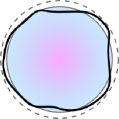
Refer to caption
(a) The vesicle fluctuates around the average shaded spherical shell. The dashed line represents the reference sphere. Note that udelimited-⟨⟩𝑢\langle u\rangle is negative.
Refer to caption
(b) Force exchanged through an infinitesimal cut at θ𝜃\theta constant. The length of the projected cut is Rsinθdϕ𝑅𝜃𝑑italic-ϕR\sin\theta d\phi, while the true length of the membrane is indicated in red.
Figure 4.4: The vesicle is represented by a solid thick line, while the reference sphere is represented in with a dashed line.

The effective tension τ𝜏\tau is the average force per unit length that is exchanged tangentially to the shell’s surface. Because of the spherical symmetry, τ𝜏\tau depends neither on the point (θ,ϕ)𝜃italic-ϕ(\theta,\phi) nor in the direction in which it is calculated. Let us thus consider an infinitesimal cut with θ𝜃\theta constant of extension dϕ𝑑italic-ϕd\phi. The component along 𝒆θsubscript𝒆𝜃\bm{e}_{\theta} of the force exchanged through the cut is on average d𝒇=Σθθdϕ𝑑𝒇delimited-⟨⟩subscriptΣ𝜃𝜃𝑑italic-ϕd\bm{f}=\langle\Sigma_{\theta\theta}\,d\phi\rangle. The length of the cut is on average R(1+u)sinθdϕdelimited-⟨⟩𝑅1𝑢𝜃𝑑italic-ϕ\langle R(1+u)\sin\theta\,d\phi\rangle. Hence,

τ=ΣθθRsinθ(1+u).𝜏delimited-⟨⟩subscriptΣ𝜃𝜃𝑅𝜃1delimited-⟨⟩𝑢\tau=\frac{\langle\Sigma_{\theta\theta}\rangle}{R\sin\theta(1+\langle u\rangle)}\,. (4.58)

Since Σθθ=σRsinθ+𝒪(u)subscriptΣ𝜃𝜃𝜎𝑅𝜃𝒪𝑢\Sigma_{\theta\theta}=\sigma R\sin\theta+\mathcal{O}(u), we obtain equivalently

τ=1RsinθΣθθσu+𝒪(u3).𝜏1𝑅𝜃delimited-⟨⟩subscriptΣ𝜃𝜃𝜎delimited-⟨⟩𝑢𝒪superscript𝑢3\tau=\frac{1}{R\sin\theta}\langle\Sigma_{\theta\theta}\rangle-\sigma\langle u\rangle+\mathcal{O}(u^{3})\,. (4.59)

Using eq.(4.2), the results presented in section 4.3.1 and in appendix F, we obtain for closed vesicles

τclosedsubscript𝜏closed\displaystyle\tau_{\mathrm{closed}} =\displaystyle= σkBTκ8πR2l=2L(l+2)(l+1)l(l1)(2l+1)H~l,𝜎subscript𝑘B𝑇𝜅8𝜋superscript𝑅2superscriptsubscript𝑙2𝐿𝑙2𝑙1𝑙𝑙12𝑙1subscript~𝐻𝑙\displaystyle\sigma-\frac{k_{\mathrm{B}}T\kappa}{8\pi R^{2}}\sum_{l=2}^{L}\frac{(l+2)(l+1)l(l-1)(2l+1)}{\tilde{H}_{l}}\,, (4.60)
=\displaystyle= σkBT8πR2l=2Ll(l+1)(2l+1)l2+l+σ¯.𝜎subscript𝑘B𝑇8𝜋superscript𝑅2superscriptsubscript𝑙2𝐿𝑙𝑙12𝑙1superscript𝑙2𝑙¯𝜎\displaystyle\sigma-\frac{k_{\mathrm{B}}T}{8\pi R^{2}}\sum_{l=2}^{L}\frac{l(l+1)(2l+1)}{l^{2}+l+\bar{\sigma}}\,. (4.61)

Note that the terms on udelimited-⟨⟩𝑢\langle u\rangle vanish and, as expected, τclosedsubscript𝜏closed\tau_{\mathrm{closed}} is independent of the point (θ,ϕ)𝜃italic-ϕ(\theta,\phi) in which it is calculated. It is interesting to examine τclosedsubscript𝜏closed\tau_{\mathrm{closed}} in the limit of large vesicles. In this case, the sum on eq.(4.61) may be substituted by an integral:

τclosedσsubscript𝜏closed𝜎\displaystyle\tau_{\mathrm{closed}}-\sigma \displaystyle\approx kBT8πR22RΛ(l+1)l(2l+1)l2+l+σ¯,subscript𝑘B𝑇8𝜋superscript𝑅2superscriptsubscript2𝑅Λ𝑙1𝑙2𝑙1superscript𝑙2𝑙¯𝜎\displaystyle-\frac{k_{\mathrm{B}}T}{8\pi R^{2}}\int_{2}^{R\Lambda}\frac{(l+1)l(2l+1)}{l^{2}+l+\bar{\sigma}}\,, (4.62)
\displaystyle\approx kBTΛ28π[1σκΛ2log(1+κΛ2σ)]+𝒪(ΛR).subscript𝑘B𝑇superscriptΛ28𝜋delimited-[]1𝜎𝜅superscriptΛ21𝜅superscriptΛ2𝜎𝒪Λ𝑅\displaystyle-\frac{k_{\mathrm{B}}T\,\Lambda^{2}}{8\pi}\left[1-\frac{\sigma}{\kappa\Lambda^{2}}\log\left(1+\frac{\kappa\Lambda^{2}}{\sigma}\right)\right]+\mathcal{O}\left(\frac{\Lambda}{R}\right)\,.

The dominant term in eq.(4.62) correctly matches the difference τσ𝜏𝜎\tau-\sigma for flat membranes given in chapter 2, eq.(2.10).

We have also calculated the normal and orthogonal components of the tension. Both vanish: Σrθ=0delimited-⟨⟩subscriptΣ𝑟𝜃0\langle\Sigma_{r\theta}\rangle=0 and Σϕθ=0delimited-⟨⟩subscriptΣitalic-ϕ𝜃0\langle\Sigma_{\phi\theta}\rangle=0. While the latter result is obvious on symmetry grounds, the former one is interesting, implying that the shell mentioned above can indeed be considered as a purely tense surface. This would probably not hold for a vesicle with non-spherical average shape. As a consequence, the Laplace law can be used without curvature corrections for a fluctuating quasi-spherical vesicle, provided that one uses τ𝜏\tau instead of σ𝜎\sigma. Indeed, this could be expected from renormalization arguments, since the Laplace law is exact (despite the curvature energy) for a perfectly spherical membrane [74].

4.4 Poked vesicles

The route to obtain τpokedsubscript𝜏poked\tau_{\mathrm{poked}} is the same as with a closed vesicle, with some minor changes. We remind that the reference sphere in poked vesicles is the sphere where u=0delimited-⟨⟩𝑢0\langle u\rangle=0, since there is no constraint on volume. Accordingly, instead of eq.(4.37), we have simply u0,0=0subscript𝑢000u_{0,0}=0. The Hamiltonian in the Gaussian approximation becomes

=4πR2σ+12ωH~l|ul,m|2+𝒪(u3),4𝜋superscript𝑅2𝜎12subscript𝜔superscriptsubscript~𝐻𝑙superscriptsubscript𝑢𝑙𝑚2𝒪superscript𝑢3\mathcal{H}=4\pi R^{2}\sigma+\frac{1}{2}\sum_{\omega}\tilde{H}_{l}^{\prime}\,|u_{l,m}|^{2}+\mathcal{O}(u^{3})\,, (4.63)

where H~l=H~l+4κσ¯subscriptsuperscript~𝐻𝑙subscript~𝐻𝑙4𝜅¯𝜎\tilde{H}^{\prime}_{l}=\tilde{H}_{l}+4\kappa\bar{\sigma} [72]. The correlations given in section 4.3.1 and in appendix F remain correct, provided one replaces H~lsubscript~𝐻𝑙\tilde{H}_{l} by H~l+4κσ¯subscript~𝐻𝑙4𝜅¯𝜎\tilde{H}_{l}+4\kappa\bar{\sigma}. Note that u2u0delimited-⟨⟩superscript𝑢2delimited-⟨⟩𝑢0\langle u^{2}\rangle\neq\langle u\rangle\equiv 0 here and that, differently from the case of closed vesicles, one must have σ¯[3,[\bar{\sigma}\in[-3,\infty[ in order to assure that correlations are positive. The discussion about the cutoff of section 4.3.1 remains valid for poked vesicles and the validity condition for the Gaussian approximation given in eq.(4.51) becomes

u2=kBT4πκl=2L2l+1(l+2)(l1)(l2+l+σ¯)+4σ¯Umax2.delimited-⟨⟩superscript𝑢2subscript𝑘B𝑇4𝜋𝜅superscriptsubscript𝑙2𝐿2𝑙1𝑙2𝑙1superscript𝑙2𝑙¯𝜎4¯𝜎superscriptsubscript𝑈𝑚𝑎𝑥2\langle u^{2}\rangle=\frac{k_{\mathrm{B}}T}{4\pi\kappa}\sum_{l=2}^{L}\frac{2l+1}{(l+2)(l-1)(l^{2}+l+\bar{\sigma})+4\bar{\sigma}}\leq U_{max}^{2}\,. (4.64)

With the same Umax=5%subscript𝑈maxpercent5U_{\mathrm{max}}=5\% as before, we have σ¯min2subscript¯𝜎min2\bar{\sigma}_{\mathrm{min}}\approx-2 for poked vesicles. The average area is given by eq.(LABEL:eq_2_area_1) with u0,0=0delimited-⟨⟩subscript𝑢000\langle u_{0,0}\rangle=0, yielding

A=4πR2+kBTR22ωl2+l+2H~l+4κσ¯.delimited-⟨⟩𝐴4𝜋superscript𝑅2subscript𝑘B𝑇superscript𝑅22subscript𝜔superscript𝑙2𝑙2subscript~𝐻𝑙4𝜅¯𝜎\langle A\rangle=4\pi R^{2}+\frac{k_{\mathrm{B}}T\,R^{2}}{2}\sum_{\omega}\frac{l^{2}+l+2}{\tilde{H}_{l}+4\kappa\bar{\sigma}}\,. (4.65)

Consequently,

αpoked=kBT8πκl=2L(l2+l+2)(2l+1)(l1)(l+2)(l2+l+σ¯)+4σ¯.subscript𝛼pokedsubscript𝑘B𝑇8𝜋𝜅superscriptsubscript𝑙2𝐿superscript𝑙2𝑙22𝑙1𝑙1𝑙2superscript𝑙2𝑙¯𝜎4¯𝜎\alpha_{\mathrm{poked}}=\frac{k_{\mathrm{B}}T}{8\pi\kappa}\sum_{l=2}^{L}\frac{(l^{2}+l+2)(2l+1)}{(l-1)(l+2)(l^{2}+l+\bar{\sigma})+4\bar{\sigma}}\,. (4.66)

Fig. 4.5 shows αmaxsubscript𝛼max\alpha_{\mathrm{max}}, i. e., αpokedsubscript𝛼poked\alpha_{\mathrm{poked}} with σ¯=2¯𝜎2\bar{\sigma}=-2, as a function of the vesicle’s radius. The excess area is somewhat larger than in the case of closed vesicles, but the general behavior is the same.
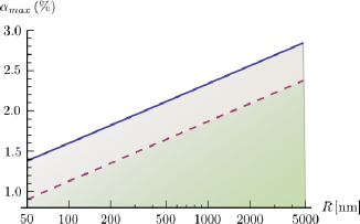
Refer to caption
Figure 4.5: The blue line stands for the maximum excess area corresponding to u2=0.05delimited-⟨⟩superscript𝑢20.05\sqrt{\langle u^{2}\rangle}=0.05 for poked vesicles, while the red dashed line stands closed vesicles. In abscissa is the vesicle’s radius. Here, Λ15nmsimilar-to-or-equalssuperscriptΛ15nm\Lambda^{-1}\simeq 5\,\mathrm{nm} and κ=25kBT𝜅25subscript𝑘B𝑇\kappa=25\,k_{\mathrm{B}}T.

Eq.(4.60), which gives τclosedsubscript𝜏closed\tau_{\mathrm{closed}} by the stress tensor method, is valid whatever the form of H~lsubscript~𝐻𝑙\tilde{H}_{l}, since τ𝜏\tau bears no term on u𝑢u. Hence, we need just to replace H~lsubscript~𝐻𝑙\tilde{H}_{l} by H~l+4κσ¯subscript~𝐻𝑙4𝜅¯𝜎\tilde{H}_{l}+4\kappa\bar{\sigma}, which yields:

τpoked=σkBT8πR2l=2Ll(l+1)(2l+1)l2+l+σ¯+4σ¯(l1)(l+2).subscript𝜏poked𝜎subscript𝑘𝐵𝑇8𝜋superscript𝑅2superscriptsubscript𝑙2𝐿𝑙𝑙12𝑙1superscript𝑙2𝑙¯𝜎4¯𝜎𝑙1𝑙2\tau_{\mathrm{poked}}=\sigma-\frac{k_{B}T}{8\pi R^{2}}\sum_{l=2}^{L}\frac{l\left({l+1}\right)\left({2l+1}\right)}{l^{2}+l+\bar{\sigma}+\frac{4\bar{\sigma}}{\left({l-1}\right)\left({l+2}\right)}}\,. (4.67)

In the limit of large vesicles, we recover again the result for flat membranes.

4.5 Discussion on τ𝜏\tau for closed and poked vesicles

We show in Fig. 4.6 the behavior of στ𝜎𝜏\sigma-\tau as a function of the Lagrange multiplier σ𝜎\sigma for closed and poked vesicles, as well as the limiting case of planar membranes. First of all, although eqs.(4.67) and (4.61) differ mathematically, it turns out that their difference as a function of σ𝜎\sigma is numerically irrelevant (see Fig. 4.6). Indeed the extra term 4σ¯/[(l1)(l+2)]4¯𝜎delimited-[]𝑙1𝑙24\bar{\sigma}/[(l-1)(l+2)] in the denominator of eq.(4.67) is only important for small l𝑙l’s, while the sum is dominated by large l𝑙l’s.

Refer to caption
Figure 4.6: Difference between the Lagrange multiplier σ𝜎\sigma and the effective mechanical tension τ𝜏\tau as a function of σ𝜎\sigma for κ=1019J𝜅superscript1019J\kappa=10^{-19}\,\mathrm{J}, kBT=4×10²¹Jsubscript𝑘B𝑇4superscript1021Jk_{\mathrm{B}}T=4\times 10^{-21}\,\mathrm{J} and Λ1=5nmsuperscriptΛ15nm\Lambda^{-1}=5\,\mathrm{nm}. The colored solid lines correspond to closed vesicles of R=50nm𝑅50nmR=50\,\mathrm{nm} (blue) and R=0.5μm𝑅0.5𝜇𝑚R=0.5\,\mu m (red), whereas the corresponding colored dashed lines represent the results for a poked vesicle. The end-points indicate the limit beyond which our Gaussian approximation is no longer valid according to section 4.3.1 (circles) or according to the discussion in section 4.4 (stars). The thick gray line corresponds to a flat membrane (eq.(4.62)).

This representation is however not very useful, since σ𝜎\sigma is not a control parameter. The most physical representation is shown in Fig. 4.7, where we see the behavior of τ𝜏\tau as a function of the excess area α𝛼\alpha. We show also the limiting case R𝑅R\rightarrow\infty. In this case, the relation between α𝛼\alpha and σ𝜎\sigma is analytical and given in eq.(2.71). In the limit of large membranes, we obtain

σ=κΛ2e8πβκα1.𝜎𝜅superscriptΛ2superscript𝑒8𝜋𝛽𝜅𝛼1\sigma=\frac{\kappa\Lambda^{2}}{e^{8\pi\beta\kappa\alpha}-1}\,. (4.68)

Applying this result to eq.(4.1), we obtain an analytical expression for τ𝜏\tau as a function of the area excess, given by

τflat(α)=κΛ2(1+α)e8πβκα1kBTΛ28π.subscript𝜏flat𝛼𝜅superscriptΛ21𝛼superscript𝑒8𝜋𝛽𝜅𝛼1subscript𝑘B𝑇superscriptΛ28𝜋\tau_{\mathrm{flat}}(\alpha)=\frac{\kappa\Lambda^{2}(1+\alpha)}{e^{8\pi\beta\kappa\alpha}-1}-\frac{k_{\mathrm{B}}T\Lambda^{2}}{8\pi}\,. (4.69)

For vesicles, α𝛼\alpha given in eq.(4.57) (or in eq.(4.66)) is numerically inverted in order to obtain σ(α)𝜎𝛼\sigma(\alpha). The result is then applied to eq.(4.61) (respectively, eq.(4.67)), yielding the curves of Fig 4.7.
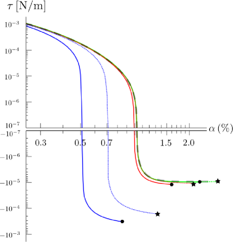
Refer to caption
Figure 4.7: Effective mechanical tension τ𝜏\tau as a function of the excess area α𝛼\alpha for κ=1019J𝜅superscript1019J\kappa=10^{-19}\,\mathrm{J}, kBT=4×10²¹Jsubscript𝑘B𝑇4superscript1021Jk_{\mathrm{B}}T=4\times 10^{-21}\,\mathrm{J} and Λ1=5nmsuperscriptΛ15nm\Lambda^{-1}=5\,\mathrm{nm}. The colored solid lines correspond to closed vesicles of R=50nm𝑅50nmR=50\,\mathrm{nm} (blue leftmost curves), R=0.5μm𝑅0.5𝜇𝑚R=0.5\,\mu m (red central curves) and R=5μm𝑅5𝜇𝑚R=5\,\mu m (green rightmost curves), while the corresponding dotted lines represent τpokedsubscript𝜏poked\tau_{\mathrm{poked}}. The end-points/stars indicate the limit beyond which our Gaussian approximation is no longer valid. The gray dashed line corresponds to the flat membrane limit given in eq.(4.69).

There are several salient points:

  1. 1.

    Even though τclosedsubscript𝜏closed\tau_{\mathrm{closed}} and τpokedsubscript𝜏poked\tau_{\mathrm{poked}} are almost indistinguishable as a function of σ𝜎\sigma, αclosedsubscript𝛼closed\alpha_{\mathrm{closed}} and αpokedsubscript𝛼poked\alpha_{\mathrm{poked}} present different dependences in terms of σ𝜎\sigma, as shown in Fig. 4.8, especially for small values of R𝑅R. This indicates that the volume constraint affects mainly the excess area and explains the differences shown in Fig. 4.7.
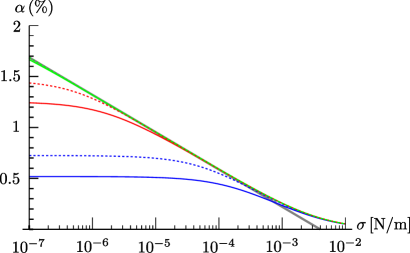
    Refer to caption
    Figure 4.8: Solid/dashed lines stand for the excess area for closed/poked vesicles for R=50nm𝑅50nmR=50\,\mathrm{nm} (blue lower curves), R=0.5μm𝑅0.5𝜇𝑚R=0.5\,\mu m (red central curves) and R=5μm𝑅5𝜇𝑚R=5\,\mu m (green upper curves). The limit of large planar membranes is shown in gray. Curves for κ=1019J𝜅superscript1019J\kappa=10^{-19}\,\mathrm{J}, kBT=4×10²¹Jsubscript𝑘B𝑇4superscript1021Jk_{\mathrm{B}}T=4\times 10^{-21}\,\mathrm{J} and Λ1=5nmsuperscriptΛ15nm\Lambda^{-1}=5\,\mathrm{nm}.
  2. 2.

    The results for τ𝜏\tau deviate from the flat limit (R𝑅R\rightarrow\infty) essentially for R1μm𝑅1𝜇𝑚R\leq 1\mu m for both closed and poked vesicles (see Fig. 4.7). Consequently, for GUVs, one is allowed to use simply the relation given in eq.(4.1). Moreover, for small tensions, it is justified to assume τσσ0similar-to-or-equals𝜏𝜎subscript𝜎0\tau\simeq\sigma-\sigma_{0}, justifying the assumptions made on [87] and presented in section 2.5.2.

  3. 3.

    Negative and quite large values of τ𝜏\tau are indeed accessible within the validity range of our Gaussian analysis in both cases (see Fig. 4.9).
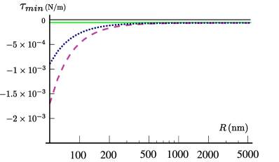
    Refer to caption
    Figure 4.9: Largest negative tension within our validity condition (for Umax=5%subscript𝑈𝑚𝑎𝑥percent5U_{max}=5\%) as a function of the vesicle’s radius for κ=1019J𝜅superscript1019J\kappa=10^{-19}\,\mathrm{J}, kBT=4×10²¹Jsubscript𝑘B𝑇4superscript1021Jk_{\mathrm{B}}T=4\times 10^{-21}\,\mathrm{J} and Λ1=5nmsuperscriptΛ15nm\Lambda^{-1}=5\,\mathrm{nm}. The violet dashed line stands for closed vesicles, while the blue dotted one stands for poked vesicles. The green solid line represents the smallest value of τ𝜏\tau for the limit of large planar membranes.

    From Fig. 4.9, we note that the biggest negative tension τminsubscript𝜏min\tau_{\mathrm{min}} that GUVs (with R1μm𝑅1𝜇mR\geq 1\mathrm{\mu m}) may sustain coincide with the biggest negative tension that large planar membranes sustain:

    τmin=kBTΛ28π.subscript𝜏minsubscript𝑘B𝑇superscriptΛ28𝜋\tau_{\mathrm{min}}=-\frac{k_{\mathrm{B}}T\,\Lambda^{2}}{8\pi}\,. (4.70)

    Depending on the uncertainty on the value of the cutoff, τminsubscript𝜏min\tau_{\mathrm{min}} may be of order 106N/msuperscript106Nm-10^{-6}\,\mathrm{N/m} or 105N/msuperscript105Nm-10^{-5}\,\mathrm{N/m}.

    Let’s recall the Young–Laplace equation

    ΔP=PinnerPouter=τ(1R1+1R2),Δ𝑃subscript𝑃innersubscript𝑃outer𝜏1subscript𝑅11subscript𝑅2\Delta P=P_{\mathrm{inner}}-P_{\mathrm{outer}}=\tau\left(\frac{1}{R_{1}}+\frac{1}{R_{2}}\right)\,, (4.71)

    where Pinner/outersubscript𝑃innerouterP_{\mathrm{inner/outer}} is, respectively, the inner and the outer pressure of the vesicle, R1subscript𝑅1R_{1} and R2subscript𝑅2R_{2} are the two principal radii (R1=R2subscript𝑅1subscript𝑅2R_{1}=R_{2} in the spherical case). As our analysis shows that τ𝜏\tau may indeed become negative, this would imply that vesicles could sustain an inner pressure lower than the outer pressure. For liquid drops, this situation is impossible, since the surface tension is a true material constant always positive.

    The possibility to sustain negative tensions, or negative pressure differences, might be experimentally investigated: i) by controlling the outer osmotic pressure, in the case of small vesicles, or ii) by poking a giant vesicle with a micropipette to which it would adhere and gently decreasing its inner pressure.

  4. 4.

    τ𝜏\tau has a plateau at large values of α𝛼\alpha for both closed and poked vesicles, which probably corresponds to the actual transition to oblate shapes: when τ𝜏\tau reaches a critical value τc<0subscript𝜏𝑐0\tau_{c}<0, the excess area rises dramatically. For small closed vesicles we find roughly τcR2/κ5subscript𝜏𝑐superscript𝑅2𝜅5\tau_{c}R^{2}/\kappa\approx-5 while for giant closed vesicles it is given by τckBTΛ2/(8π)similar-to-or-equalssubscript𝜏𝑐subscript𝑘B𝑇superscriptΛ28𝜋\tau_{c}\simeq-k_{\mathrm{B}}T\Lambda^{2}/(8\pi), i. e., below the mean-field threshold (see discussion after eq.(4.41)). The high symmetry phase (spherical vesicle) is thus stabilized by its entropic fluctuations, as one might have expected.

    Experimentally, this transition might be tested by controlling the pressure outside the vesicle. Indeed, applying the Young–Laplace pressure formula given in eq.(4.71) for a vesicle of radius R𝑅R and at τcsubscript𝜏𝑐\tau_{c}, we find that the critical pressure difference yielding the shape transition is ΔPcsup[10κ/R3,kBTΛ2/(4πR)]Δsubscript𝑃𝑐supremum10𝜅superscript𝑅3subscript𝑘B𝑇superscriptΛ24𝜋𝑅\Delta P_{c}\approx-\sup[10\kappa/R^{3},k_{\mathrm{B}}T\Lambda^{2}/(4\pi R)]. Numerically, for a closed spherical vesicle with κ=25kBT𝜅25subscript𝑘B𝑇\kappa=25\,k_{\mathrm{B}}T, T=300K𝑇300𝐾T=300\,K and Λ=(1/5nm)Λ15nm\Lambda=(1/5\,\mathrm{nm}), we find ΔPc= 8×10³PaΔsubscript𝑃𝑐8superscript103Pa\Delta P_{c}=-\,8\times 10^{3}\,\mathrm{Pa} and ΔPc=25PaΔsubscript𝑃𝑐25Pa\Delta P_{c}=-25\,\mathrm{Pa}, for vesicles with radius 50nm50nm50\,\mathrm{nm} and 5μm5𝜇m5\,\mathrm{\mu m}, respectively.

  5. 5.

    There exists a well defined excess area α0subscript𝛼0\alpha_{0} corresponding to a vanishing lateral tension τ=0𝜏0\tau=0 (see Fig. 4.10). This corresponds to the case where the pressure difference between the inner and the outer media vanishes. Its value is very much radius dependent for R1μm𝑅1𝜇𝑚R\leq 1\,\mu m, but one recovers for R2μm𝑅2𝜇𝑚R\geq 2\,\mu m the flat membrane limit given in eq.(2.76).
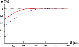
    Refer to caption
    Figure 4.10: Spontaneous excess area α0subscript𝛼0\alpha_{0}, corresponding to τ=0𝜏0\tau=0, as a function of the vesicle radius for closed (blue dashed line) and poked (red solid line) vesicles. The dotted horizontal line gives the flat membrane limit. The material parameters are the same as in Fig. 4.7.

4.6 Derivation of τ𝜏\tau using the free-energy

For a flat membrane, one may also obtain τ𝜏\tau by differentiating the free-energy with respect to the projected area Apsubscript𝐴𝑝A_{p}, as we have shown in section 2.2 [72],[2], [3], but there are two pitfalls. One must: i) take the thermodynamic limit Apsubscript𝐴𝑝A_{p}\to\infty only after the differentiation, and ii) introduce a variation of the cutoff in order that the total number of modes remains constant during the differentiation, as discussed in [3].

Let us investigate the free-energy method in the case of quasi-spherical vesicles. The free-energy, \mathcal{F}, is given by

=1βln𝒟[𝒓]eβ,1𝛽𝒟delimited-[]𝒓superscript𝑒𝛽\mathcal{F}=-\frac{1}{\beta}\ln\!\int\!\mathcal{D}[\bm{r}]\,e^{-\beta\mathcal{H}}, (4.72)

the integral running over all the configurations of the vesicle. At the Gaussian level and for closed vesicles, \mathcal{H} is given in terms of spherical harmonics by eq.(4.39), and since 𝒓=R𝒆r+Ru(θ,ϕ)𝒆r𝒓𝑅subscript𝒆𝑟𝑅𝑢𝜃italic-ϕsubscript𝒆𝑟\bm{r}=R\,\bm{e}_{r}+R\,u(\theta,\phi)\,\bm{e}_{r}, we may write (in agreement with ref. [60]):

𝒟[𝒓]=l=2L(m=0lRdul,m)(m=1lRdul,m),𝒟delimited-[]𝒓superscriptsubscriptproduct𝑙2𝐿superscriptsubscriptproduct𝑚0𝑙𝑅𝑑superscriptsubscript𝑢𝑙𝑚superscriptsubscriptproduct𝑚1𝑙𝑅𝑑superscriptsubscript𝑢𝑙𝑚\displaystyle\mathcal{D}[\bm{r}]=\prod_{l=2}^{L}\left({\prod_{m=0}^{l}\,R\,du_{l,m}^{\mathcal{R}}}\right)\left({\prod_{m=1}^{l}\,R\,du_{l,m}^{\mathcal{I}}}\right), (4.73)

where the superscripts \mathcal{R} and \mathcal{I} signify real part and imaginary part, respectively. This measure corresponds to the so-called normal gauge, which is known to be correct for small fluctuations [60]. We note that the radius R𝑅R of the reference sphere appears explicitly and that for each value of l𝑙l, only half of the allowed values of m𝑚m have to be considered, as 𝐫𝐫\mathbf{r} is real. Performing the Gaussian integrals, one obtains

=4πR2σ+kBTl=2L2l+12ln(βH~lR2).4𝜋superscript𝑅2𝜎subscript𝑘𝐵𝑇superscriptsubscript𝑙2𝐿2𝑙12𝛽subscript~𝐻𝑙superscript𝑅2\mathcal{F}=4\pi R^{2}\sigma+k_{B}T\sum_{l=2}^{L}\frac{2l+1}{2}\ln\left({\frac{\beta\widetilde{H}_{l}}{R^{2}}}\right)\,. (4.74)

In order to obtain τclosedsubscript𝜏closed\tau_{\mathrm{closed}}, we must differentiate \mathcal{F} with respect to the vesicle’s “projected area" Apsubscript𝐴𝑝A_{p}. Which one, however? The area AV=4πR2subscript𝐴𝑉4𝜋superscript𝑅2A_{V}=4\pi R^{2} of the reference sphere (i.e., the sphere having the same volume as the vesicle’s), or the area of the vesicle’s average shape, defined as Am=4πR(1+u)2subscript𝐴𝑚4𝜋superscriptdelimited-⟨⟩𝑅1𝑢2A_{m}=4\pi\langle R(1+u)\rangle^{2}? It will turn out that the former choice is the correct one. In a sense, this is natural because it corresponds to our parametrization. However, it is not that obvious, because the definition of τclosedsubscript𝜏closed\tau_{\mathrm{closed}} in eq.(4.58) involves the area of the average vesicle’s shape.

Let us thus pick Ap=AV4πR2subscript𝐴𝑝subscript𝐴𝑉4𝜋superscript𝑅2A_{p}=A_{V}\equiv 4\pi R^{2}. It is worth noticing that H~lsubscript~𝐻𝑙\widetilde{H}_{l} depends on Apsubscript𝐴𝑝A_{p} only through σ¯=σR2/κ¯𝜎𝜎superscript𝑅2𝜅\bar{\sigma}=\sigma R^{2}/\kappa, yielding

H~lR2=(l1)(l+2)σ.subscript~𝐻𝑙superscript𝑅2𝑙1𝑙2𝜎\frac{\partial\widetilde{H}_{l}}{\partial R^{2}}=\left({l-1}\right)\left({l+2}\right)\sigma\,. (4.75)

With this choice:

τclosed=Ap=14πR2,subscript𝜏closedsubscript𝐴𝑝14𝜋superscript𝑅2\tau_{\mathrm{closed}}=\frac{\partial\mathcal{F}}{\partial A_{p}}=\frac{1}{4\pi}\frac{\partial\mathcal{F}}{\partial R^{2}}\,, (4.76)

we obtain

τclosed=σkBT8πR2l=2Ll(l+1)(2l+1)l2+l+σ¯,subscript𝜏closed𝜎subscript𝑘𝐵𝑇8𝜋superscript𝑅2superscriptsubscript𝑙2𝐿𝑙𝑙12𝑙1superscript𝑙2𝑙¯𝜎\tau_{\mathrm{closed}}=\sigma-\frac{k_{B}T}{8\pi R^{2}}\sum_{l=2}^{L}\frac{l\left({l+1}\right)\left({2l+1}\right)}{l^{2}+l+\bar{\sigma}}\,, (4.77)

which is identical to the result obtained from the stress tensor approach, eq.(4.61). How about the pitfalls mentioned above? First, we didn’t take the thermodynamic limit before differentiating. Actually, this would not be problematic, since the quantification of the modes does not involve the size of the system, like it is the case for planar membranes. Second, we have kept L𝐿L (hence the number of modes) constant during the differentiation, in agreement with the fact that L=4+R2Λ21𝐿4superscript𝑅2superscriptΛ21L=\lfloor\sqrt{4+R^{2}\Lambda^{2}}-1\rfloor is constant for a mathematically infinitesimal change of R𝑅R.

We may obtain a more intrinsic expression for τclosedsubscript𝜏closed\tau_{\mathrm{closed}}. With A=Ap(1+α)delimited-⟨⟩𝐴subscript𝐴𝑝1𝛼\left<{A}\right>=A_{p}\,(1+\alpha), and Nmodes=l=2L(2l+1)subscript𝑁modessuperscriptsubscript𝑙2𝐿2𝑙1N_{\mathrm{modes}}=\sum_{l=2}^{L}(2l+1), we may rewrite τclosedsubscript𝜏closed\tau_{\mathrm{closed}} as

τclosedAp=AσkBT2Nmodes.subscript𝜏closedsubscript𝐴𝑝delimited-⟨⟩𝐴𝜎subscript𝑘𝐵𝑇2subscript𝑁modes\tau_{\mathrm{closed}}\,A_{p}=\left<{A}\right>\sigma-\frac{k_{B}T}{2}N_{\mathrm{modes}}\,. (4.78)

The quickest way to obtain this result is to keep separate, when differentiating with respect to R2superscript𝑅2R^{2}, the two terms coming from ln(H~l)subscript~𝐻𝑙\ln(\tilde{H}_{l}) and ln(1/R2)1superscript𝑅2\ln(1/R^{2}) in eq.(4.74). The interpretation of this equation is not straightforward, because 12kBT12subscript𝑘B𝑇\frac{1}{2}k_{\mathrm{B}}T is the internal energy per mode (not the free-energy per mode). Note that the same form for τ𝜏\tau is also valid in the planar case, as shown in [3].

In addition, let’s see what happens if we take Ap=Am4πR2(1+u)2subscript𝐴𝑝subscript𝐴𝑚4𝜋superscript𝑅2superscript1delimited-⟨⟩𝑢2A_{p}=A_{m}\equiv 4\pi R^{2}(1+\langle u\rangle)^{2}:

τAm=Ap=AV(AmAV)1subscript𝜏subscript𝐴𝑚subscript𝐴𝑝subscript𝐴𝑉superscriptsubscript𝐴𝑚subscript𝐴𝑉1\tau_{A_{m}}=\frac{\partial\mathcal{F}}{\partial A_{p}}=\frac{\partial\mathcal{F}}{\partial A_{V}}\left(\frac{\partial A_{m}}{\partial A_{V}}\right)^{-1}\, (4.79)

where we remind AV=4πR2subscript𝐴𝑉4𝜋superscript𝑅2A_{V}=4\pi R^{2}. Using u=u2delimited-⟨⟩𝑢delimited-⟨⟩superscript𝑢2\langle u\rangle=-\langle u^{2}\rangle, one obtains

(AmAV)1=11u2=1+u2+𝒪(u3).superscriptsubscript𝐴𝑚subscript𝐴𝑉111delimited-⟨⟩superscript𝑢21delimited-⟨⟩superscript𝑢2𝒪superscript𝑢3\left(\frac{\partial A_{m}}{\partial A_{V}}\right)^{-1}=\frac{1}{1-\langle u^{2}\rangle}=1+\langle u^{2}\rangle+\mathcal{O}(u^{3})\,. (4.80)

Clearly, differentiating with respect to Amsubscript𝐴𝑚A_{m} yields supplemental terms of order u2superscript𝑢2u^{2} The result is thus wrong, in the sense that it differs from the result obtained by the stress tensor method.

Let’s now re-derive eq.(4.67) by deriving the free-energy. In the case of poked vesicles, it is given by the same expression as eq.(4.74) with H~lsubscript~𝐻𝑙\tilde{H}_{l} replaced by H~lsubscriptsuperscript~𝐻𝑙\tilde{H}^{\prime}_{l}:

=4πR2σ+kBTl=2L2l+12ln(βH~lR2).superscript4𝜋superscript𝑅2𝜎subscript𝑘B𝑇superscriptsubscript𝑙2𝐿2𝑙12𝛽subscriptsuperscript~𝐻𝑙superscript𝑅2\mathcal{F^{\prime}}=4\pi R^{2}\sigma+k_{\mathrm{B}}T\sum_{l=2}^{L}\frac{2l+1}{2}\ln\left(\frac{\beta\tilde{H}^{\prime}_{l}}{R^{2}}\right)\,. (4.81)

It turns out, again, that τpoked=/(4πR2)subscript𝜏pokedsuperscript4𝜋superscript𝑅2\tau_{\mathrm{poked}}=\partial\mathcal{F}^{\prime}/\partial(4\pi R^{2}) exactly. This result is satisfying, but at the same time it shows how slippery the free-energy approach can be: differentiating with respect to the area of the average vesicle is correct in the case of poked vesicles but not in the case of closed vesicles. The stress tensor method is thus a much safer.

Our expression for τpokedsubscript𝜏poked\tau_{\mathrm{poked}} differs from that obtained in ref.[72], where the authors considered also a quasi-spherical membrane without volume constraint. In particular, the mechanical tension obtained in that reference cannot take negative values. We believe that the discrepancy between the two results comes from the omission in ref.[72] of the factors R𝑅R within the measure. Indeed the factor 1/R21superscript𝑅21/R^{2} in the logarithm of our eq.(4.81) is absent in the corresponding expression (A.9) of ref.[72].

4.7 In a nutshell

In this chapter, we have compared the mechanical tension τ𝜏\tau one applies by aspiring a vesicle with a micropipette, for instance, with the tension σ𝜎\sigma theoretically introduced in the Hamiltonian to fix the membrane’s area in the case of quasi-spherical vesicles. We have studied both the case of usual closed vesicles and the case of poked vesicles, free to exchange liquid with the outer media. We conclude that in both cases, for GUVs, the relation between τ𝜏\tau and σ𝜎\sigma is very well approximated by the relation obtained in the case of planar membranes, given in eq.(4.1). Accordingly, for GUVs under small tensions, we can assume simply τσσ0similar-to-or-equals𝜏𝜎subscript𝜎0\tau\simeq\sigma-\sigma_{0}, as in the case of planar membranes. Moreover, in both cases, we predict the possibility of an internal pressure smaller than the outer, situation impossible in the case of liquid drops. Regarding comparatively the behavior of closed and poked vesicles, we expect the excess area of both to differ for small vesicles. At last, we have shown that the concept of projected area for vesicles is not clear. Thus, we conclude that it is much safer to derive τ𝜏\tau by averaging the projected stress tensor.

Part III Nanotubes of membrane

Chapter 5 Force needed to extract a fluctuating nanotube

In this and in the following chapter, we shall study the membrane nanotubes presented in section 1.4.4. The main results of both chapters were obtained with Jean-Baptiste Fournier and were published in [6]. As we have seen, these tubes are very thin, with a radius ranging from dozens up to hundreds of nanometers, while their length may achieve micrometers. They are very current in living cells and seem to play an important role in cell transport and communication [92].

In laboratory, nanotubes can be extracted by applying very localized forces to membranes. In Fig. 1.36 of chapter 1, we have presented a brief sum-up of the more popular methods used to extract nanotubes. Here we interest ourselves in the force needed to extract (and hold) these tubes, which can be precisely measured in experiments using optical tweezer. The experimental procedure in this case consists in attaching a small glass bead to a vesicle held by a micropipette [96][100]. A laser is pointed to the glass bead, which is thus attracted to the center of the beam with a force that depends linearly on the distance between the bead and the center of the beam. In experiments, one displaces the position of the center of the beam, denoted xtrapsubscript𝑥trapx_{\mathrm{trap}}, while measuring the position x𝑥x of the bead, as shown in Fig. 5.1. One then deduces the applied force through f=ktrap(xxtrap)𝑓subscript𝑘trap𝑥subscript𝑥trapf=-k_{\mathrm{trap}}(x-x_{\mathrm{trap}}), where ktrapsubscript𝑘trapk_{\mathrm{trap}} is a constant that characterizes the stiffness of the optical trap.

Refer to caption
Figure 5.1: Extraction of nanotubes using optical tweezers. The laser beam, represented in red, traps the glass bead attached to the membrane (in blue). The laser is then displaced and a tube is pulled. By controlling the position of the center of the laser beam xtrapsubscript𝑥trapx_{\mathrm{trap}} and of the bead x𝑥x, one deduces the applied force in the direction of the extracted tube.

Remark that usually, as in the case of Fig. 5.1, one measures only the force in the axis of the tube, which is by symmetry the only component with non-vanishing average. Note also that nanotubes are not stable: if one stops applying the point force, the membrane will evolve to a less curve configuration and the tube will be re-absorbed in the vesicle.

Former theoretical works studied both the formation mechanism of nanotubes [102], [112] and their (dynamical) stability [113], [114],  [115]. As nanotubes are very thin compared to the GUVs from which they are usually pulled, it is usually assumed that the vesicle acts as a lipid reservoir to the tube. In this case, as discussed in refs. [102] and  [112], one can neglect the pressure difference across the tube. The effective energy superscript\mathcal{H}^{\prime} is thus simply given by the Helfrich Hamiltonian (eq.(1.15)) plus the work of the force that keeps the tube. For a symmetrical membrane, i. e., a membrane whose spontaneous curvature vanishes, the energy for a perfectly cylindrical tube with radius R𝑅R and length L𝐿L is [102]

=(κ2R2+σ)2πRLfL.superscript𝜅2superscript𝑅2𝜎2𝜋𝑅𝐿𝑓𝐿\mathcal{H}^{\prime}=\left(\frac{\kappa}{2R^{2}}+\sigma\right)2\pi RL-fL\,. (5.1)

where κ𝜅\kappa is the bending rigidity and σ𝜎\sigma is the Lagrange multiplier associated to the microscopical area of the membrane, which we remind is not directly measurable. The energy coming from the Gaussian curvature is omitted, since we do not consider topological changes. Minimizing this energy with respect to R𝑅R and L𝐿L, one obtains, respectively

R0=κ2σsubscript𝑅0𝜅2𝜎R_{0}=\sqrt{\frac{\kappa}{2\sigma}} (5.2)

and

f0=2π2κσ.subscript𝑓02𝜋2𝜅𝜎f_{0}=2\pi\sqrt{2\kappa\sigma}\,. (5.3)

These values correspond to the mean-field values of the radius and of the force needed to hold a tube, in the sense that thermal fluctuations relatives to the cylindrical shape were totally neglected.

At first glance, one may think that neglecting the effects of thermal fluctuations is largely justified, since it is a reasonable assumption for planar membranes: as the correlation length is σ1/2proportional-toabsentsuperscript𝜎12\propto\sigma^{-1/2}, fluctuations are quickly suppressed as the tension increases [112]. Recently, however, it has been shown that the tubular geometry implied a substantially different behavior: tubes should present very strong shape fluctuations due to a one-dimensional set of extremely soft modes (Goldstone modes, see Fig. 5.2[7].

Refer to caption
Figure 5.2: The first soft, Goldstone modes [7].

Accordingly, it is natural to ask how the average force along the tube’s axis f𝑓f, taking into account its fluctuations, differs from the mean-field value f0subscript𝑓0f_{0}. It is our aim this chapter to settle this question. To do so, we follow roughly the same steps as in the last chapter, starting by introducing the parametrization and the energy in 5.1. Afterwards, we shall derive the projected stress tensor for quasi-cylindrical geometry in section 5.2. As this calculation is totally new, we propose some verifications in the same section. In section 5.3, we average the stress tensor and evaluate f𝑓f. At last, in section 5.4, we compare f𝑓f with f0subscript𝑓0f_{0} and discuss in which cases one is allowed to assume ff0similar-to-or-equals𝑓subscript𝑓0f\simeq f_{0}. There we discuss also experimental consequences and re-interpret the curve shown in Fig. 1.37.

5.1 Parametrization and Hamiltonian

We shall restrict our attention to deformed tubes weakly departing from the cylinder corresponding the mean-field approximation whose radius, as we have shown above, is given by

R0=κ2σ.subscript𝑅0𝜅2𝜎R_{0}=\sqrt{\frac{\kappa}{2\sigma}}\,. (5.4)

Let’s consider a cylindrical coordinate system (O;r,θ,z)𝑂𝑟𝜃𝑧(O;r,\theta,z) aligned with the tube (see Fig. 5.3).

Refer to caption
Figure 5.3: Parametrization of the fluctuating tube (thick line). The thin solid line represents the reference cylinder with radius R0subscript𝑅0R_{0}.

The shape of the fluctuating tube is parametrized by

𝒓(ρ,z)=R0[1+u(ρ,z)]𝒆r(ρ)+z𝒆z,𝒓𝜌𝑧subscript𝑅0delimited-[]1𝑢𝜌𝑧subscript𝒆𝑟𝜌𝑧subscript𝒆𝑧\bm{r}(\rho,z)=R_{0}\left[1+u(\rho,z)\right]\bm{e}_{r}(\rho)+z\,\bm{e}_{z}\,, (5.5)

with u1much-less-than𝑢1u\ll 1 and z[0,L]𝑧0𝐿z\in[0,L], where L𝐿L is the total length of the tube. Note that instead of θ𝜃\theta, we have used ρ=R0θ[0,2πR0]𝜌subscript𝑅0𝜃02𝜋subscript𝑅0\rho=R_{0}\,\theta\in[0,2\pi R_{0}], in order to have u𝑢u as a function of two variables with the same dimension.

We shall consider the situation of a relatively short tubule extracted from a giant vesicle of radius RvesR0much-greater-thansubscript𝑅vessubscript𝑅0R_{\mathrm{ves}}\gg R_{0} (or from a vesicle connected to a lipid reservoir), so that each monolayer of the tubule is actually exchanging material with a very large reservoir and the standard Helfrich model (see section 1.3) is sufficient for the calculation of equilibrium and statistical properties [102][112]. As we do not consider topology changes, the Hamiltonian is simply given by

=S(σ+κ2H2)𝑑A,subscript𝑆𝜎𝜅2superscript𝐻2differential-d𝐴\mathcal{H}=\int_{S}\left(\sigma+\frac{\kappa}{2}H^{2}\right)\,dA\,, (5.6)

where S𝑆S is the tube’s surface. Note that taking into account the area-difference elasticity, as is done in the ADE𝐴𝐷𝐸ADE model, is essential in the situation where very long tubules are extracted from small vesicles [116], or when studying the formation of small tethered vesicles under the action of an axial load [117]. Remark also that one should usually consider the pressure difference across the membrane by adding a term ΔPVΔ𝑃𝑉-\Delta P\,V to the Hamiltonian, where V𝑉V is the volume of the tube and ΔP=PinPoutΔ𝑃subscript𝑃insubscript𝑃out\Delta P=P_{\mathrm{in}}-P_{\mathrm{out}}, with Pinsubscript𝑃inP_{\mathrm{in}} (resp. Poutsubscript𝑃outP_{\mathrm{out}}) is the pressure inside (resp. outside) the vesicle from which the tube is extracted. From the Young-Laplace equation (eq.(1.35)), ΔPΔ𝑃\Delta P relates to the vesicle’s radius and tension through ΔP=2τ/RvesΔ𝑃2𝜏subscript𝑅ves\Delta P=2\tau/R_{\mathrm{ves}}. Let’s compare the contribution of this term with the contribution coming the term proportional to σ𝜎\sigma for a tube of radius RRvesmuch-less-than𝑅subscript𝑅vesR\ll R_{\mathrm{ves}} and length L𝐿L:

ΔPVσA=ΔPπR2Lσ 2πRL=τσ×RRves1,Δ𝑃𝑉𝜎𝐴Δ𝑃𝜋superscript𝑅2𝐿𝜎2𝜋𝑅𝐿𝜏𝜎𝑅subscript𝑅vesmuch-less-than1\frac{\Delta P\,V}{\sigma\,A}=\frac{\Delta P\,\pi R^{2}\,L}{\sigma\,2\pi R\,L}=\frac{\tau}{\sigma}\times\frac{R}{R_{\mathrm{ves}}}\ll 1\,, (5.7)

since we are extracting tubes far smaller than the vesicle and since τ<σ𝜏𝜎\tau<\sigma. It is justified thus to neglect the pressure difference across the tubule [102][112].

Differential geometry yields the general dA𝑑𝐴dA given in eq.(4.4) and H𝐻H given in eq.(4.9). For the case of quasi-cylindrical geometry, we obtain up to order two on u𝑢u

Ωh(u,{ui},{uij})𝑑ρ𝑑z,similar-to-or-equalssubscriptΩ𝑢subscript𝑢𝑖subscript𝑢𝑖𝑗differential-d𝜌differential-d𝑧\mathcal{H}\simeq\int_{\Omega}h(u,\{u_{i}\},\{u_{ij}\})\,d\rho\,dz, (5.8)

where i,j{ρ,z}𝑖𝑗𝜌𝑧i,j\in\{\rho,z\}, uiiu=u/isubscript𝑢𝑖subscript𝑖𝑢𝑢𝑖u_{i}\equiv\partial_{i}u=\partial u/\partial i, ΩΩ\Omega corresponds to the domain of the reference cylinder of radius R0subscript𝑅0R_{0} over which the membrane stands, and [7]

h\displaystyle h =\displaystyle= σ[2+u22R02(uρρ+uzz)+R04(uρρ+uzz)2\displaystyle\sigma\left[2+u^{2}-2\,R_{0}^{2}\,(u_{\rho\rho}+u_{zz})+R_{0}^{4}\,(u_{\rho\rho}+u_{zz})^{2}\right. (5.9)
+\displaystyle+ 2R02uρ2+4R02uuρρ]+𝒪(u3).\displaystyle\left.2\,R_{0}^{2}\,u_{\rho}^{2}+4\,R_{0}^{2}\,u\,u_{\rho\rho}\right]+\mathcal{O}(u^{3}).

5.2 Derivation of the stress tensor for a cylindrical
geometry

In analogy to the planar and quasi-spherical cases, the projected stress tensor relates linearly the force that the region 111 exerts over region 222 to the length of the projected cut d𝑑d\ell through

dϕ12=𝚺𝒎d,𝑑subscriptbold-italic-ϕ12𝚺𝒎𝑑d\bm{\phi}_{\mathrm{1\rightarrow 2}}=\bm{\Sigma}\cdot\bm{m}\,d\ell\,, (5.10)

where 𝒎=mρ𝒆ρ+mz𝒆z𝒎subscript𝑚𝜌subscript𝒆𝜌subscript𝑚𝑧subscript𝒆𝑧\bm{m}=m_{\rho}\,\bm{e}_{\rho}+m_{z}\,\bm{e}_{z} is the normal to the cut on the reference cylinder (see Fig 5.4).
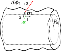
Refer to caption
Figure 5.4: The upper vector in red represents the three-dimensional force exchanged through an infinitesimal cut on the membrane. In green, we see the projection of the cut onto the reference cylinder. Note that the vector 𝒎𝒎\bm{m}, normal to the projected cut, is contained on the reference cylinder (dashed lines).

In order to derive 𝚺𝚺\bm{\Sigma}, we consider at each point of the membrane an arbitrary infinitesimal displacement δ𝒂=δaρ𝒆ρ+δaz𝒆z+δar𝒆r𝛿𝒂𝛿subscript𝑎𝜌subscript𝒆𝜌𝛿subscript𝑎𝑧subscript𝒆𝑧𝛿subscript𝑎𝑟subscript𝒆𝑟\delta\bm{a}=\delta a_{\rho}\,\bm{e}_{\rho}+\delta a_{z}\,\bm{e}_{z}+\delta a_{r}\,\bm{e}_{r} corresponding to a variation (δρ,δz)𝛿𝜌𝛿𝑧(\delta\rho,\delta z) on the projected cylinder (see Fig. 5.5). Accordingly, the membrane’s shape becomes u~(ρ,z)=u(ρ,z)+δu(ρ,z)~𝑢𝜌𝑧𝑢𝜌𝑧𝛿𝑢𝜌𝑧\tilde{u}(\rho,z)=u(\rho,z)+\delta u(\rho,z).

Refer to caption
(a) Coordinate space used in the parametrization of the tube’s shape. The shaded area represents ΩΩ\Omega, the thick solid line represents ΩΩ\partial\Omega and the dashed line represents ΩΩ\partial\Omega after an infinitesimal displacement δ𝒂𝛿𝒂\delta\bm{a} of the membrane. The line in the center represents the projected cut.
Refer to caption
(b) Fluctuating tube before (shaded) and after (dashed red) a general displacement. The reference cylinder is shown by the dashed black line.
Figure 5.5: Deriving the projected stress tensor.

As one can see in Fig. 5.5(b), the new edge’s position satisfies R0[1+u~(ρ+δρ,z+δz)]𝒆r(ρ+δρ)+(z+δz)𝒆z=R0[1+u(ρ,z)]𝒆r(ρ)+z𝒆z+δ𝒂subscript𝑅0delimited-[]1~𝑢𝜌𝛿𝜌𝑧𝛿𝑧subscript𝒆𝑟𝜌𝛿𝜌𝑧𝛿𝑧subscript𝒆𝑧subscript𝑅0delimited-[]1𝑢𝜌𝑧subscript𝒆𝑟𝜌𝑧subscript𝒆𝑧𝛿𝒂R_{0}[1+\tilde{u}(\rho+\delta\rho,z+\delta z)]\,\bm{e}_{r}(\rho+\delta\rho)+(z+\delta z)\,\bm{e}_{z}=R_{0}[1+u(\rho,z)]\,\bm{e}_{r}(\rho)+z\,\bm{e}_{z}+\delta\bm{a}, which implies

δaρ𝛿subscript𝑎𝜌\displaystyle\delta a_{\rho} =\displaystyle= δρ(1+u),𝛿𝜌1𝑢\displaystyle\delta\rho\left(1+u\right), (5.11)
δaz𝛿subscript𝑎𝑧\displaystyle\delta a_{z} =\displaystyle= δz,𝛿𝑧\displaystyle\delta z\,, (5.12)
δar𝛿subscript𝑎𝑟\displaystyle\delta a_{r} =\displaystyle= R0(δu+uzδz+uρδρ).subscript𝑅0𝛿𝑢subscript𝑢𝑧𝛿𝑧subscript𝑢𝜌𝛿𝜌\displaystyle R_{0}\left(\delta u+u_{z}\delta z+u_{\rho}\delta\rho\right). (5.13)

We now impose that δ𝒂𝛿𝒂\delta\bm{a} is done at fixed orientation of the membrane’s normal: in this way, only the boundary forces work, not the torques. The normal to the membrane is 𝒏=𝒕ρ×𝒕z/|𝒕ρ×𝒕z|𝒏subscript𝒕𝜌subscript𝒕𝑧subscript𝒕𝜌subscript𝒕𝑧\bm{n}=\bm{t}_{\rho}\times\bm{t}_{z}/|\bm{t}_{\rho}\times\bm{t}_{z}|, with 𝒕ρ=ρ𝒓=R0uρ𝒆r+(1+u)𝒆ρsubscript𝒕𝜌subscript𝜌𝒓subscript𝑅0subscript𝑢𝜌subscript𝒆𝑟1𝑢subscript𝒆𝜌\bm{t}_{\rho}=\partial_{\rho}\bm{r}=R_{0}\,u_{\rho}\,\bm{e}_{r}+(1+u)\,\bm{e}_{\rho} and 𝒕z=z𝒓=R0uz𝒆r+𝒆zsubscript𝒕𝑧subscript𝑧𝒓subscript𝑅0subscript𝑢𝑧subscript𝒆𝑟subscript𝒆𝑧\bm{t}_{z}=\partial_{z}\bm{r}=R_{0}\,u_{z}\,\bm{e}_{r}+\bm{e}_{z}. This gives 𝒏=[1R02(uρ2+uz2)/2]𝒆r(ρ)+R0(u1)uρ𝒆ρ(ρ)R0uz𝒆z+𝒪(u3)𝒏delimited-[]1superscriptsubscript𝑅02superscriptsubscript𝑢𝜌2superscriptsubscript𝑢𝑧22subscript𝒆𝑟𝜌subscript𝑅0𝑢1subscript𝑢𝜌subscript𝒆𝜌𝜌subscript𝑅0subscript𝑢𝑧subscript𝒆𝑧𝒪superscript𝑢3\bm{n}=\left[1-R_{0}^{2}\left(u_{\rho}^{2}+u_{z}^{2}\right)/2\right]\,\bm{e}_{r}(\rho)+R_{0}\left(u-1\right)\,u_{\rho}\,\bm{e}_{\rho}(\rho)-R_{0}\,u_{z}\,\bm{e}_{z}+\mathcal{O}(u^{3}). The normal variation is given by δ𝒏=𝒏~(ρ+δρ,z+δz)𝒏(ρ,z)𝛿𝒏~𝒏𝜌𝛿𝜌𝑧𝛿𝑧𝒏𝜌𝑧\delta\bm{n}=\tilde{\bm{n}}(\rho+\delta\rho,z+\delta z)-\bm{n}(\rho,z), 𝒏~~𝒏\tilde{\bm{n}} being the analog of 𝒏𝒏\bm{n} for u~~𝑢\tilde{u} instead of u𝑢u. In order to impose δ𝒏=0𝛿𝒏0\delta\bm{n}=0, we require that δ𝒏𝒕ρ=0𝛿𝒏subscript𝒕𝜌0\delta\bm{n}\cdot\bm{t}_{\rho}=0 and δ𝒏𝒕z=0𝛿𝒏subscript𝒕𝑧0\delta\bm{n}\cdot\bm{t}_{z}=0, yielding, up to order u2superscript𝑢2u^{2}

δuz𝛿subscript𝑢𝑧\displaystyle\delta u_{z} =\displaystyle= (uzuρuρz)δρuzzδz,subscript𝑢𝑧subscript𝑢𝜌subscript𝑢𝜌𝑧𝛿𝜌subscript𝑢𝑧𝑧𝛿𝑧\displaystyle\left(u_{z}\,u_{\rho}-u_{\rho z}\right)\delta\rho-u_{zz}\,\delta z\,,
δuρ𝛿subscript𝑢𝜌\displaystyle\delta u_{\rho} =\displaystyle= [R02(1+u)+2uρ2uρρ]δρdelimited-[]superscriptsubscript𝑅021𝑢2superscriptsubscript𝑢𝜌2subscript𝑢𝜌𝜌𝛿𝜌\displaystyle\left[R_{0}^{-2}\left(1+u\right)+2\,u_{\rho}^{2}-u_{\rho\rho}\right]\delta\rho (5.15)
+\displaystyle+ (uzuρuρz)δz+uρδu.subscript𝑢𝑧subscript𝑢𝜌subscript𝑢𝜌𝑧𝛿𝑧subscript𝑢𝜌𝛿𝑢\displaystyle\left(u_{z}\,u_{\rho}-u_{\rho z}\right)\delta z+u_{\rho}\,\delta u\,.

Using eqs.(5.11)–(5.15), we may now express the variations {δρ,δz,δu,δuρ,δuz}𝛿𝜌𝛿𝑧𝛿𝑢𝛿subscript𝑢𝜌𝛿subscript𝑢𝑧\{\delta\rho,\delta z,\delta u,\delta u_{\rho},\delta u_{z}\} at the boundary in terms of the components of δ𝒂𝛿𝒂\delta\bm{a}. We obtain, to order u2superscript𝑢2u^{2}

δρ𝛿𝜌\displaystyle\delta\rho =\displaystyle= (1u+u2)δaρ,1𝑢superscript𝑢2𝛿subscript𝑎𝜌\displaystyle\left(1-u+u^{2}\right)\delta a_{\rho}\,, (5.16)
δz𝛿𝑧\displaystyle\delta z =\displaystyle= δaz,𝛿subscript𝑎𝑧\displaystyle\delta a_{z}\,, (5.17)
δu𝛿𝑢\displaystyle\delta u =\displaystyle= (u1)uρδaρuzδaz+R01δar,𝑢1subscript𝑢𝜌𝛿subscript𝑎𝜌subscript𝑢𝑧𝛿subscript𝑎𝑧superscriptsubscript𝑅01𝛿subscript𝑎𝑟\displaystyle(u-1)u_{\rho}\,\delta a_{\rho}-u_{z}\,\delta a_{z}+R_{0}^{-1}\,\delta a_{r}\,, (5.18)
δuρ𝛿subscript𝑢𝜌\displaystyle\delta u_{\rho} =\displaystyle= [R02+uρ2+(u1)uρρ]δaρdelimited-[]superscriptsubscript𝑅02superscriptsubscript𝑢𝜌2𝑢1subscript𝑢𝜌𝜌𝛿subscript𝑎𝜌\displaystyle\left[R_{0}^{-2}+u_{\rho}^{2}+\left(u-1\right)u_{\rho\rho}\right]\,\delta a_{\rho} (5.19)
\displaystyle- uρzδaz+R01(1u)uρδar,subscript𝑢𝜌𝑧𝛿subscript𝑎𝑧superscriptsubscript𝑅011𝑢subscript𝑢𝜌𝛿subscript𝑎𝑟\displaystyle u_{\rho z}\,\delta a_{z}+R_{0}^{-1}\left(1-u\right)u_{\rho}\,\delta a_{r}\,,
δuz𝛿subscript𝑢𝑧\displaystyle\delta u_{z} =\displaystyle= [uρuz+(u1)uρz]δaρuzzδaz.delimited-[]subscript𝑢𝜌subscript𝑢𝑧𝑢1subscript𝑢𝜌𝑧𝛿subscript𝑎𝜌subscript𝑢𝑧𝑧𝛿subscript𝑎𝑧\displaystyle\left[u_{\rho}\,u_{z}+\left(u-1\right)u_{\rho z}\right]\,\delta a_{\rho}-u_{zz}\,\delta a_{z}\,. (5.20)

To obtain 𝚺𝚺\bm{\Sigma}, we study the variation of the energy after the displacement δ𝒂𝛿𝒂\delta\bm{a}. On the one hand, in terms of hh, one has

δbulk=Ω[hui(hui)+ij(huij)]𝑑ρ𝑑z𝛿subscriptbulksubscriptΩdelimited-[]𝑢subscript𝑖subscript𝑢𝑖subscript𝑖subscript𝑗subscript𝑢𝑖𝑗differential-d𝜌differential-d𝑧\delta\mathcal{H}_{\mathrm{bulk}}=\int_{\Omega}\left[\frac{\partial h}{\partial u}-\partial_{i}\left(\frac{\partial h}{\partial u_{i}}\right)+\partial_{i}\partial_{j}\left(\frac{\partial h}{\partial u_{ij}}\right)\right]\,d\rho\,dz\, (5.21)

for the bulk of the membrane and

δboundary=Ωmi[hδi+(huijhuij)δu+huijδuj]𝑑,𝛿subscriptboundarysubscriptΩsubscript𝑚𝑖delimited-[]𝛿𝑖subscript𝑢𝑖subscript𝑗subscript𝑢𝑖𝑗𝛿𝑢subscript𝑢𝑖𝑗𝛿subscript𝑢𝑗differential-d\delta\mathcal{H}_{\mathrm{boundary}}=\int_{\partial\Omega}\!m_{i}\left[h\,\delta i+\left(\frac{\partial h}{\partial u_{i}}-\partial_{j}\frac{\partial h}{\partial u_{ij}}\right)\delta u+\frac{\partial h}{\partial u_{ij}}\,\delta u_{j}\right]d\ell\,, (5.22)

for the boundary energy variation. On the other hand, the work of forces at the boundary is given by

δboundary=Ωδ𝒂𝚺𝒎𝑑.𝛿subscriptboundarysubscriptΩ𝛿𝒂𝚺𝒎differential-d\delta\mathcal{H}_{\mathrm{boundary}}=\!\!\int_{\partial\Omega}\!\delta\bm{a}\cdot\bm{\Sigma}\cdot\bm{m}\,d\ell\,. (5.23)

By comparing the last two equations, we obtain ΣzisubscriptΣ𝑧𝑖\Sigma_{zi}, ΣrisubscriptΣ𝑟𝑖\Sigma_{ri} and ΣρisubscriptΣ𝜌𝑖\Sigma_{\rho i} (i𝑖i being either ρ𝜌\rho or z𝑧z):

ΣzisubscriptΣ𝑧𝑖\displaystyle\Sigma_{zi} =\displaystyle= hδzi(huijhuij)uzhuiρuρzhuizuzz+𝒪(u3),subscript𝛿𝑧𝑖subscript𝑢𝑖subscript𝑗subscript𝑢𝑖𝑗subscript𝑢𝑧subscript𝑢𝑖𝜌subscript𝑢𝜌𝑧subscript𝑢𝑖𝑧subscript𝑢𝑧𝑧𝒪superscript𝑢3\displaystyle h\,\delta_{zi}-\left(\frac{\partial h}{\partial u_{i}}-\partial_{j}\frac{\partial h}{\partial u_{ij}}\right)u_{z}-\frac{\partial h}{\partial u_{i\rho}}\,u_{\rho z}-\frac{\partial h}{\partial u_{iz}}\,u_{zz}+\mathcal{O}(u^{3})\,, (5.24)
ΣrisubscriptΣ𝑟𝑖\displaystyle\Sigma_{ri} =\displaystyle= 1R0(huijhuij)+1R0(1u)huiρuρ+𝒪(u3),1subscript𝑅0subscript𝑢𝑖subscript𝑗subscript𝑢𝑖𝑗1subscript𝑅01𝑢subscript𝑢𝑖𝜌subscript𝑢𝜌𝒪superscript𝑢3\displaystyle\frac{1}{R_{0}}\left(\frac{\partial h}{\partial u_{i}}-\partial_{j}\frac{\partial h}{\partial u_{ij}}\right)+\frac{1}{R_{0}}\left(1-u\right)\frac{\partial h}{\partial u_{i\rho}}\,u_{\rho}+\mathcal{O}(u^{3})\,, (5.25)
ΣρisubscriptΣ𝜌𝑖\displaystyle\Sigma_{\rho i} =\displaystyle= (1u+u2)hδρi+(huijhuij)(u1)uρ1𝑢superscript𝑢2subscript𝛿𝜌𝑖subscript𝑢𝑖subscript𝑗subscript𝑢𝑖𝑗𝑢1subscript𝑢𝜌\displaystyle\left(1-u+u^{2}\right)h\,\delta_{\rho i}+\left(\frac{\partial h}{\partial u_{i}}-\partial_{j}\frac{\partial h}{\partial u_{ij}}\right)\left(u-1\right)u_{\rho}
+\displaystyle+ huiz[uρuz+(u1)uρz]+huiρ[1R02+uρ2+(u1)uρρ]+𝒪(u3).subscript𝑢𝑖𝑧delimited-[]subscript𝑢𝜌subscript𝑢𝑧𝑢1subscript𝑢𝜌𝑧subscript𝑢𝑖𝜌delimited-[]1superscriptsubscript𝑅02superscriptsubscript𝑢𝜌2𝑢1subscript𝑢𝜌𝜌𝒪superscript𝑢3\displaystyle\frac{\partial h}{\partial u_{iz}}\left[u_{\rho}\,u_{z}+\left(u-1\right)u_{\rho z}\right]+\frac{\partial h}{\partial u_{i\rho}}\left[\frac{1}{R_{0}^{2}}+u_{\rho}^{2}+\left(u-1\right)u_{\rho\rho}\right]+\mathcal{O}(u^{3})\,.

Note that due to the presence of terms such as R02h/uiρsuperscriptsubscript𝑅02subscript𝑢𝑖𝜌R_{0}^{-2}\,\partial h/\partial u_{i\rho} (see, e.g., the expression of ΣρisubscriptΣ𝜌𝑖\Sigma_{\rho i}), it is in general necessary to have hh at 𝒪(u3)𝒪superscript𝑢3\mathcal{O}(u^{3}) in order to get the stress components at 𝒪(u2)𝒪superscript𝑢2\mathcal{O}(u^{2}). This means adding

h3subscript3\displaystyle h_{3} =\displaystyle= u3R02(6uuρρ+5uρ2uz2)usuperscript𝑢3superscriptsubscript𝑅026𝑢subscript𝑢𝜌𝜌5superscriptsubscript𝑢𝜌2superscriptsubscript𝑢𝑧2𝑢\displaystyle-u^{3}-R_{0}^{2}\,\left(6\,u\,u_{\rho\rho}+5\,u_{\rho}^{2}-u_{z}^{2}\right)\,u (5.27)
+\displaystyle+ R04(uzz23uρρ22uzzuρρ)+4R04uρuzuρzsuperscriptsubscript𝑅04superscriptsubscript𝑢𝑧𝑧23superscriptsubscript𝑢𝜌𝜌22subscript𝑢𝑧𝑧subscript𝑢𝜌𝜌4superscriptsubscript𝑅04subscript𝑢𝜌subscript𝑢𝑧subscript𝑢𝜌𝑧\displaystyle R_{0}^{4}\left(u_{zz}^{2}-3\,u_{\rho\rho}^{2}-2\,u_{zz}\,u_{\rho\rho}\right)+4\,R_{0}^{4}\,u_{\rho}\,u_{z}\,u_{\rho z}
+\displaystyle+ R04(uρρuzz)uρ2+R04(uρρ+3uzz)uz2superscriptsubscript𝑅04subscript𝑢𝜌𝜌subscript𝑢𝑧𝑧superscriptsubscript𝑢𝜌2superscriptsubscript𝑅04subscript𝑢𝜌𝜌3subscript𝑢𝑧𝑧superscriptsubscript𝑢𝑧2\displaystyle R_{0}^{4}\left(u_{\rho\rho}-u_{zz}\right)u_{\rho}^{2}+R_{0}^{4}\left(u_{\rho\rho}+3u_{zz}\right)u_{z}^{2}

to hh given in eq.(5.9) before evaluating the derivatives in eqs.(5.24)–(5.2). For ΣzisubscriptΣ𝑧𝑖\Sigma_{zi}, however, one may check the 𝒪(u2)𝒪superscript𝑢2\mathcal{O}(u^{2}) terms in hh are sufficient. Explicitly, we obtain up to order two on u𝑢u

ΣzzsubscriptΣ𝑧𝑧\displaystyle\Sigma_{zz} =\displaystyle= σ{2+u2+2R02[uρ2+(2u1)uρρ]\displaystyle\sigma\left\{2+u^{2}+2R_{0}^{2}\left[u_{\rho}^{2}+\left(2u-1\right)u_{\rho\rho}\right]\right. (5.28)
+\displaystyle+ R04[uρρ2uzz2+2uz(uzzz+uρρz)]},\displaystyle R_{0}^{4}\left.\left[u_{\rho\rho}^{2}-u_{zz}^{2}+2u_{z}\left(u_{zzz}+u_{\rho\rho z}\right)\right]\right\}\,,
ΣzρsubscriptΣ𝑧𝜌\displaystyle\Sigma_{z\rho} =\displaystyle= 2R02(12u)uρz+2R04[uz(uρzz+uρρρ)uρz(uzz+uρρ)],2superscriptsubscript𝑅0212𝑢subscript𝑢𝜌𝑧2superscriptsubscript𝑅04delimited-[]subscript𝑢𝑧subscript𝑢𝜌𝑧𝑧subscript𝑢𝜌𝜌𝜌subscript𝑢𝜌𝑧subscript𝑢𝑧𝑧subscript𝑢𝜌𝜌\displaystyle 2\,R_{0}^{2}\left(1-2\,u\right)u_{\rho z}+2\,R_{0}^{4}\left[u_{z}\left(u_{\rho zz}+u_{\rho\rho\rho}\right)-u_{\rho z}\left(u_{zz}+u_{\rho\rho}\right)\right]\,, (5.29)
ΣrzsubscriptΣ𝑟𝑧\displaystyle\Sigma_{rz} =\displaystyle= 2R0uuz2R03[(1+u)uzzz+(1u)uρρz+uzuzzuρuzρ],2subscript𝑅0𝑢subscript𝑢𝑧2superscriptsubscript𝑅03delimited-[]1𝑢subscript𝑢𝑧𝑧𝑧1𝑢subscript𝑢𝜌𝜌𝑧subscript𝑢𝑧subscript𝑢𝑧𝑧subscript𝑢𝜌subscript𝑢𝑧𝜌\displaystyle 2\,R_{0}\,u\,u_{z}-2\,R_{0}^{3}\left[\left(1+u\right)u_{zzz}+\left(1-u\right)u_{\rho\rho z}+u_{z}\,u_{zz}-u_{\rho}\,u_{z\rho}\right]\,, (5.30)
ΣrρsubscriptΣ𝑟𝜌\displaystyle\Sigma_{r\rho} =\displaystyle= 2R0(14u)uρ2subscript𝑅014𝑢subscript𝑢𝜌\displaystyle-2\,R_{0}\left(1-4\,u\right)u_{\rho} (5.31)
\displaystyle- 2R03[(13u)uρρρ+(1u)uρzz4uρuρρ+uρuzz+uzuρz],2superscriptsubscript𝑅03delimited-[]13𝑢subscript𝑢𝜌𝜌𝜌1𝑢subscript𝑢𝜌𝑧𝑧4subscript𝑢𝜌subscript𝑢𝜌𝜌subscript𝑢𝜌subscript𝑢𝑧𝑧subscript𝑢𝑧subscript𝑢𝜌𝑧\displaystyle 2\,R_{0}^{3}\,\left[\left(1-3\,u\right)u_{\rho\rho\rho}+\left(1-u\right)u_{\rho zz}-4u_{\rho}\,u_{\rho\rho}+u_{\rho}\,u_{zz}+u_{z}\,u_{\rho z}\right]\,,
ΣρzsubscriptΣ𝜌𝑧\displaystyle\Sigma_{\rho z} =\displaystyle= 2R02[(1u)uρz+uρuz]2superscriptsubscript𝑅02delimited-[]1𝑢subscript𝑢𝜌𝑧subscript𝑢𝜌subscript𝑢𝑧\displaystyle 2\,R_{0}^{2}\left[\left(1-u\right)u_{\rho z}+u_{\rho}\,u_{z}\right] (5.32)
\displaystyle- 2R04[(uzz+uρρ)uρz(uρρz+uzzz)uρ],2superscriptsubscript𝑅04delimited-[]subscript𝑢𝑧𝑧subscript𝑢𝜌𝜌subscript𝑢𝜌𝑧subscript𝑢𝜌𝜌𝑧subscript𝑢𝑧𝑧𝑧subscript𝑢𝜌\displaystyle 2\,R_{0}^{4}\left[\left(u_{zz}+u_{\rho\rho}\right)u_{\rho z}-\left(u_{\rho\rho z}+u_{zzz}\right)u_{\rho}\right]\,,
ΣρρsubscriptΣ𝜌𝜌\displaystyle\Sigma_{\rho\rho} =\displaystyle= 2u3u2+R02[uz2+uρ2+2(13u)uρρ]2𝑢3superscript𝑢2superscriptsubscript𝑅02delimited-[]superscriptsubscript𝑢𝑧2superscriptsubscript𝑢𝜌2213𝑢subscript𝑢𝜌𝜌\displaystyle 2\,u-3\,u^{2}+R_{0}^{2}\left[u_{z}^{2}+u_{\rho}^{2}+2\left(1-3\,u\right)u_{\rho\rho}\right] (5.33)
+\displaystyle+ R04[uzz2uρρ2+2(uρzz+uρρρ)uρ].superscriptsubscript𝑅04delimited-[]superscriptsubscript𝑢𝑧𝑧2superscriptsubscript𝑢𝜌𝜌22subscript𝑢𝜌𝑧𝑧subscript𝑢𝜌𝜌𝜌subscript𝑢𝜌\displaystyle R_{0}^{4}\left[u_{zz}^{2}-u_{\rho\rho}^{2}+2\left(u_{\rho zz}+u_{\rho\rho\rho}\right)u_{\rho}\right]\,.

Note that we may easily recover from ΣzzsubscriptΣ𝑧𝑧\Sigma_{zz} the mean-field force needed to hold a tubule. Indeed, u=0𝑢0u=0 yields Σzz=2σsubscriptΣ𝑧𝑧2𝜎\Sigma_{zz}=2\sigma [4], i.e., f0=2πR×2σ=2π2κσsubscript𝑓02𝜋𝑅2𝜎2𝜋2𝜅𝜎f_{0}=2\pi R\times 2\sigma=2\pi\sqrt{2\kappa\sigma}. As we have discussed in section 1.4.4, this result is very interesting: if the mechanical tension were due only to the tension σ𝜎\sigma, we should expect f0=σ×2πR0subscript𝑓0𝜎2𝜋subscript𝑅0f_{0}=\sigma\times 2\pi R_{0}. In reality, the curvature yields a supplementary term 1/2(κ/R02)12𝜅superscriptsubscript𝑅021/2\,(\kappa/R_{0}^{2}) to the mechanical tension τ𝜏\tau, which explains the factor two in our result. In the next two sections we shall propose some tests to verify the correctness of these equations.

5.2.1 Verification: stress tensor in the tangent frame

Here we propose a first check by showing that from eqs.(5.28)–(5.33), one re-obtains the stress tensor in the local frame given in eq.(1.50). We consider a general membrane, not necessarily tubular. At a general point P𝑃P of the membrane, there are two principal curvatures CXsubscript𝐶𝑋C_{X} and CYsubscript𝐶𝑌C_{Y} whose principal directions 𝒆Xsubscript𝒆𝑋\bm{e}_{X} and 𝒆Ysubscript𝒆𝑌\bm{e}_{Y} are orthogonal. We place our reference cylinder tangent to the membrane at P𝑃P, with its axis direction 𝒆zsubscript𝒆𝑧\bm{e}_{z} parallel to 𝒆Ysubscript𝒆𝑌\bm{e}_{Y} and 𝒆ρsubscript𝒆𝜌\bm{e}_{\rho} parallel to 𝒆Xsubscript𝒆𝑋\bm{e}_{X} , as shown in Fig. 5.6.

Refer to caption
Figure 5.6: The shaded surface represents a piece of membrane. The principal curvatures, as well as the principal directions 𝒆Xsubscript𝒆𝑋\bm{e}_{X} and 𝒆Ysubscript𝒆𝑌\bm{e}_{Y} in P𝑃P, are shown in red and green. The dashed cylinder represents the reference cylinder.

By geometry (see Fig. 5.7), one determines the shape of the membrane near to P𝑃P in the cylindrical coordinate system, yielding

𝒓=R0[1+12(CX+1R0)ρ2R0+12CYz2R2]𝒆r.𝒓subscript𝑅0delimited-[]112subscript𝐶𝑋1subscript𝑅0superscript𝜌2subscript𝑅012subscript𝐶𝑌superscript𝑧2superscript𝑅2subscript𝒆𝑟\bm{r}=R_{0}\,\left[1+\frac{1}{2}\left(C_{X}+\frac{1}{R_{0}}\right)\frac{\rho^{2}}{R_{0}}+\frac{1}{2}\,C_{Y}\frac{z^{2}}{R^{2}}\right]\bm{e}_{r}\,. (5.34)

Comparing eq.(5.5) and eq.(5.34), we identify

u(ρ,z)=12(CX+1R0)ρ2R0+12CYz2R2.𝑢𝜌𝑧12subscript𝐶𝑋1subscript𝑅0superscript𝜌2subscript𝑅012subscript𝐶𝑌superscript𝑧2superscript𝑅2u(\rho,z)=\frac{1}{2}\left(C_{X}+\frac{1}{R_{0}}\right)\frac{\rho^{2}}{R_{0}}+\frac{1}{2}\,C_{Y}\frac{z^{2}}{R^{2}}\,. (5.35)
Refer to caption
Figure 5.7: Schematic representation highlighting the geometrical quantities needed to determine u(ρ,z)𝑢𝜌𝑧u(\rho,z) in the plan perpendicular to 𝒆zsubscript𝒆𝑧\bm{e}_{z}.

Applying eq.(5.35) to eqs.(5.28)–(5.33), one obtains

ΣzzsubscriptΣ𝑧𝑧\displaystyle\Sigma_{zz} =\displaystyle= σκ2CY2+κ2CX2,𝜎𝜅2superscriptsubscript𝐶𝑌2𝜅2superscriptsubscript𝐶𝑋2\displaystyle\sigma-\frac{\kappa}{2}\,C_{Y}^{2}+\frac{\kappa}{2}\,C_{X}^{2}\,, (5.36)
ΣρρsubscriptΣ𝜌𝜌\displaystyle\Sigma_{\rho\rho} =\displaystyle= σ+κ2CY2κ2CX2,𝜎𝜅2superscriptsubscript𝐶𝑌2𝜅2superscriptsubscript𝐶𝑋2\displaystyle\sigma+\frac{\kappa}{2}\,C_{Y}^{2}-\frac{\kappa}{2}\,C_{X}^{2}\,, (5.37)
ΣrzsubscriptΣ𝑟𝑧\displaystyle\Sigma_{rz} =\displaystyle= κCz,𝜅𝐶𝑧\displaystyle-\kappa\,\frac{\partial C}{\partial z}\,, (5.38)
ΣrρsubscriptΣ𝑟𝜌\displaystyle\Sigma_{r\rho} =\displaystyle= κCρ,𝜅𝐶𝜌\displaystyle-\kappa\,\frac{\partial C}{\partial\rho}\,, (5.39)
ΣzρsubscriptΣ𝑧𝜌\displaystyle\Sigma_{z\rho} =\displaystyle= 0,0\displaystyle 0\,, (5.40)
ΣρzsubscriptΣ𝜌𝑧\displaystyle\Sigma_{\rho z} =\displaystyle= 0,0\displaystyle 0\,, (5.41)

where C=CX+CY𝐶subscript𝐶𝑋subscript𝐶𝑌C=C_{X}+C_{Y} is the total curvature. Noting that we have the equivalences Xρ𝑋𝜌X\equiv\rho, Yz𝑌𝑧Y\equiv z and Zr𝑍𝑟Z\equiv r near P𝑃P, these equations are identical to eq.(1.50).

5.2.2 Verification: force between two rings constraining the tube

In order to control the validity of the formula giving ΣzzsubscriptΣ𝑧𝑧\Sigma_{zz}, which will be the only component used in the next sections, let us calculate the force acting between two “undulating rings" separated by a distance L𝐿L (see Fig. 5.8) by deriving the free-energy and compare to the force obtained using the projected stress tensor.
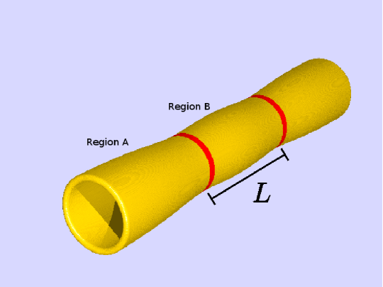
Refer to caption
Figure 5.8: Tube constrained by two rings separated by a distance L𝐿L. We have also considered the case of “undulating rings”. The region A𝐴A goes from very far to the first ring up to it, while the region B𝐵B stands for the region between the rings.

The rings are described by the boundary conditions

u(ρ,±L/2)=U0cos(nρR),𝑢𝜌plus-or-minus𝐿2subscript𝑈0𝑛𝜌𝑅u(\rho,\pm L/2)=U_{0}\,\cos\left(\frac{n\rho}{R}\right)\,, (5.42)

and zu(ρ,±L/2)=0subscript𝑧𝑢𝜌plus-or-minus𝐿20\partial_{z}u(\rho,\pm L/2)=0, for n>1𝑛1n>1. By symmetry, we assume u(ρ,z)=U(z)cos(nρ/R)𝑢𝜌𝑧𝑈𝑧𝑛𝜌𝑅u(\rho,z)=U(z)\,\cos(n\rho/R). Thus the distortion energy (5.8)–(5.9) between the rings takes the form:

=πR0σL2L2[(n21)2U22n2R02UU′′+R04U′′2]𝑑z.𝜋subscript𝑅0𝜎superscriptsubscript𝐿2𝐿2delimited-[]superscriptsuperscript𝑛212superscript𝑈22superscript𝑛2superscriptsubscript𝑅02𝑈superscript𝑈′′superscriptsubscript𝑅04superscript𝑈′′2differential-d𝑧\mathcal{H}=\pi R_{0}\,\sigma\int_{-\frac{L}{2}}^{\frac{L}{2}}\left[\left(n^{2}-1\right)^{2}U^{2}-2\,n^{2}R_{0}^{2}\,U\,U^{\prime\prime}+R_{0}^{4}\,U^{\prime\prime 2}\right]\,dz\,. (5.43)

The equilibrium shape is given by the Euler-Lagrange equation given in eq.(5.21), yielding

(n21)2U(z)2n2R2U′′(z)+R4U′′′′(z)=0.superscriptsuperscript𝑛212𝑈𝑧2superscript𝑛2superscript𝑅2superscript𝑈′′𝑧superscript𝑅4superscript𝑈′′′′𝑧0(n^{2}-1)^{2}U(z)-2n^{2}R^{2}U^{\prime\prime}(z)+R^{4}U^{\prime\prime\prime\prime}(z)=0\,. (5.44)

The solution satisfying the boundary conditions is

U(z)=U0[n+sinh(n+)cosh(nz/R0)nsinh(n)cosh(n+z/R0)]A(),𝑈𝑧subscript𝑈0delimited-[]subscript𝑛subscript𝑛subscript𝑛𝑧subscript𝑅0subscript𝑛subscript𝑛subscript𝑛𝑧subscript𝑅0𝐴U(z)=U_{0}\,\frac{\left[n_{+}\sinh(n_{+}\ell)\cosh(n_{-}z/R_{0})-n_{-}\sinh(n_{-}\ell)\cosh(n_{+}z/R_{0})\right]}{A(\ell)}\,, (5.45)

where =L/(2R0)𝐿2subscript𝑅0\ell=L/(2R_{0}), A()=n+sinh(n+)cosh(n)nsinh(n)cosh(n+)𝐴subscript𝑛subscript𝑛subscript𝑛subscript𝑛subscript𝑛subscript𝑛A(\ell)=n_{+}\sinh(n_{+}\ell)\cosh(n_{-}\ell)-n_{-}\sinh(n_{-}\ell)\cosh(n_{+}\ell) and n±=(n2±2n21)1/2subscript𝑛plus-or-minussuperscriptplus-or-minussuperscript𝑛22superscript𝑛2112n_{\pm}=(n^{2}\pm\sqrt{2n^{2}-1})^{1/2}.

To evaluate the balance of the forces acting over first ring, which is symmetrical from the force acting over the second one, we have to consider the force exerted by region A𝐴A, 𝒇Asubscript𝒇𝐴\bm{f}_{A}, and the force exerted by region B𝐵B, 𝒇Bsubscript𝒇𝐵\bm{f}_{B}. Each region is in equilibrium, implying that the integral of ΣzzsubscriptΣ𝑧𝑧\Sigma_{zz} over ρ𝜌\rho is constant in each one of them. We may thus consider an arbitrary projected path with 𝒎=𝒆z𝒎subscript𝒆𝑧\bm{m}=\bm{e}_{z} in each region to evaluate forces. For the region A𝐴A, we will consider a path very far from the ring, so that u0𝑢0u\rightarrow 0. We have

𝒇Asubscript𝒇𝐴\displaystyle\bm{f}_{A} =\displaystyle= 02πR0𝚺𝒆z𝑑ρ,superscriptsubscript02𝜋subscript𝑅0𝚺subscript𝒆𝑧differential-d𝜌\displaystyle\int_{0}^{2\pi R_{0}}\bm{\Sigma}\cdot\bm{e}_{z}\,d\rho\,, (5.46)
=\displaystyle= 02πR0Σρz𝑑ρ𝒆ρ+02πR0Σrz𝑑ρ𝒆r+02πR0Σzz𝑑ρ𝒆z,superscriptsubscript02𝜋subscript𝑅0subscriptΣ𝜌𝑧differential-d𝜌subscript𝒆𝜌superscriptsubscript02𝜋subscript𝑅0subscriptΣ𝑟𝑧differential-d𝜌subscript𝒆𝑟superscriptsubscript02𝜋subscript𝑅0subscriptΣ𝑧𝑧differential-d𝜌subscript𝒆𝑧\displaystyle\int_{0}^{2\pi R_{0}}\Sigma_{\rho z}\,d\rho\,\bm{e}_{\rho}+\int_{0}^{2\pi R_{0}}\Sigma_{rz}\,d\rho\,\bm{e}_{r}+\int_{0}^{2\pi R_{0}}\Sigma_{zz}\,d\rho\,\bm{e}_{z}\,,
=\displaystyle= 02πR02σ𝑑ρ𝒆z.superscriptsubscript02𝜋subscript𝑅02𝜎differential-d𝜌subscript𝒆𝑧\displaystyle\int_{0}^{2\pi R_{0}}2\sigma\,d\rho\,\bm{e}_{z}\,.

In the last passage, we have used the fact that Σzz2σsubscriptΣ𝑧𝑧2𝜎\Sigma_{zz}\to 2\sigma, Σρz0subscriptΣ𝜌𝑧0\Sigma_{\rho z}\to 0 and Σrz0subscriptΣ𝑟𝑧0\Sigma_{rz}\to 0 as u0𝑢0u\to 0. For the region B𝐵B, we consider a path at z=0𝑧0z=0. We obtain

𝒇Bsubscript𝒇𝐵\displaystyle\bm{f}_{B} =\displaystyle= 02πR0𝚺|z=0𝒆zdρ,evaluated-atsuperscriptsubscript02𝜋subscript𝑅0𝚺𝑧0subscript𝒆𝑧𝑑𝜌\displaystyle\int_{0}^{2\pi R_{0}}\bm{\Sigma}|_{z=0}\cdot\bm{e}_{z}\,d\rho\,, (5.47)
=\displaystyle= 02πR0Σρz|z=0dρ𝒆ρ+02πR0Σrz|z=0dρ𝒆r+02πR0Σzz|z=0dρ𝒆z,evaluated-atsuperscriptsubscript02𝜋subscript𝑅0subscriptΣ𝜌𝑧𝑧0𝑑𝜌subscript𝒆𝜌evaluated-atsuperscriptsubscript02𝜋subscript𝑅0subscriptΣ𝑟𝑧𝑧0𝑑𝜌subscript𝒆𝑟evaluated-atsuperscriptsubscript02𝜋subscript𝑅0subscriptΣ𝑧𝑧𝑧0𝑑𝜌subscript𝒆𝑧\displaystyle\int_{0}^{2\pi R_{0}}\Sigma_{\rho z}|_{z=0}\,d\rho\,\bm{e}_{\rho}+\int_{0}^{2\pi R_{0}}\Sigma_{rz}|_{z=0}\,d\rho\,\bm{e}_{r}+\int_{0}^{2\pi R_{0}}\Sigma_{zz}|_{z=0}\,d\rho\,\bm{e}_{z}\,,
=\displaystyle= 02πR0Σzz|z=0dρ𝒆z.evaluated-atsuperscriptsubscript02𝜋subscript𝑅0subscriptΣ𝑧𝑧𝑧0𝑑𝜌subscript𝒆𝑧\displaystyle\int_{0}^{2\pi R_{0}}\Sigma_{zz}|_{z=0}\,d\rho\,\bm{e}_{z}\,.

The forces in the other directions, 𝒆ρsubscript𝒆𝜌\bm{e}_{\rho} and 𝒆rsubscript𝒆𝑟\bm{e}_{r}, vanish after integration, as expected given the symmetry of the system. The resulting force is then

f(L)𝒆z=𝒇A𝒇B=02πR0(2σΣzz|z=0)𝑑ρ𝒆z.𝑓𝐿subscript𝒆𝑧subscript𝒇𝐴subscript𝒇𝐵superscriptsubscript02𝜋subscript𝑅02𝜎evaluated-atsubscriptΣ𝑧𝑧𝑧0differential-d𝜌subscript𝒆𝑧f(L)\,\bm{e}_{z}=\bm{f}_{A}-\bm{f}_{B}=\int_{0}^{2\pi R_{0}}\left(2\sigma-\Sigma_{zz}|_{z=0}\right)\,d\rho\,\bm{e}_{z}\,. (5.48)

Using eq.(5.28) to calculate ΣzzsubscriptΣ𝑧𝑧\Sigma_{zz}, we obtain

f(L)=B(n21)2cosh(2n+)cosh(2n)A()2,𝑓𝐿𝐵superscriptsuperscript𝑛2122subscript𝑛2subscript𝑛𝐴superscript2f(L)=-B\left(n^{2}-1\right)^{2}\,\frac{\cosh\left(2n_{+}\ell\right)-\cosh\left(2n_{-}\ell\right)}{A(\ell)^{2}}\,, (5.49)

where B=πRσU022n21𝐵𝜋𝑅𝜎superscriptsubscript𝑈022superscript𝑛21B=\pi R\sigma U_{0}^{2}\sqrt{2n^{2}-1}. Intuitively, one should expect the rings to collapse in order to minimize the tube’s deformation. Indeed, the resulting force between the rings is always attractive.

In order to check this result, we propose ourselves to re-derive f(L)𝑓𝐿f(L) using a different method that does not involve the stress tensor. First, we will evaluate the energy stored between the rings, given in eq.(5.43). As the tube is in equilibrium, it’s shape obeys eq.(5.44). Applying this equation to the first term of eq.(5.43), we obtain

=πR05σL2L2(UU′′′′+U′′2)𝑑z.𝜋superscriptsubscript𝑅05𝜎superscriptsubscript𝐿2𝐿2𝑈superscript𝑈′′′′superscript𝑈′′2differential-d𝑧\mathcal{H}=\pi R_{0}^{5}\,\sigma\int_{-\frac{L}{2}}^{\frac{L}{2}}\left(-U\,U^{\prime\prime\prime\prime}+U^{\prime\prime 2}\right)\,dz\,. (5.50)

Integrating by parts the term on UU′′′′𝑈superscript𝑈′′′′U\,U^{\prime\prime\prime\prime} and reminding that U(z)𝑈𝑧U(z) is an even function, that U(±L/2)=U0𝑈plus-or-minus𝐿2subscript𝑈0U(\pm L/2)=U_{0} and that U(±L/2)=0superscript𝑈plus-or-minus𝐿20U^{\prime}(\pm L/2)=0, we obtain

\displaystyle\mathcal{H} =\displaystyle= 2πR05σU0U′′′(L/2),2𝜋superscriptsubscript𝑅05𝜎subscript𝑈0superscript𝑈′′′𝐿2\displaystyle 2\pi\,R_{0}^{5}\,\sigma\,U_{0}\,U^{\prime\prime\prime}(-L/2)\,, (5.51)
=\displaystyle= 4BR0n+nsinh(n+)sinh(n)A(),4𝐵subscript𝑅0subscript𝑛subscript𝑛subscript𝑛subscript𝑛𝐴\displaystyle 4BR_{0}\,\frac{n_{+}n_{-}\sinh(n_{+}\ell)\sinh(n_{-}\ell)}{A(\ell)}\,,

where we have used the solution given in eq.(5.45) to obtain the last passage. From the stored energy, the resulting force between the rings is given by

f(L)=d(L)dL.𝑓𝐿𝑑𝐿𝑑𝐿f(L)=-\frac{d\mathcal{H}(L)}{dL}\,. (5.52)

After a careful calculation, we recover the result obtained from the stress tensor (eq.(5.28)), testifying of the correctness of the component ΣzzsubscriptΣ𝑧𝑧\Sigma_{zz} of the stress tensor.

5.3 Evaluation of the average force

In order to hold a nanotube, one must apply a force exactly equivalent to the force that the rest of the fluctuating tubule exerts. Thus, considering a section of the tube with 𝒎=𝒆z𝒎subscript𝒆𝑧\bm{m}=\bm{e}_{z}, the average force needed to hold a fluctuating tube is

f𝒆z𝑓subscript𝒆𝑧\displaystyle f\,\bm{e}_{z} =\displaystyle= 02πR0𝚺𝒆z𝑑ρ,delimited-⟨⟩superscriptsubscript02𝜋subscript𝑅0𝚺subscript𝒆𝑧differential-d𝜌\displaystyle\left\langle\int_{0}^{2\pi R_{0}}\bm{\Sigma}\cdot\bm{e}_{z}\,d\rho\right\rangle\,, (5.53)
=\displaystyle= 02πR0(Σrz𝒆r+Σρz𝒆ρ+Σzz𝒆z)𝑑ρ,superscriptsubscript02𝜋subscript𝑅0delimited-⟨⟩subscriptΣ𝑟𝑧subscript𝒆𝑟delimited-⟨⟩subscriptΣ𝜌𝑧subscript𝒆𝜌delimited-⟨⟩subscriptΣ𝑧𝑧subscript𝒆𝑧differential-d𝜌\displaystyle\int_{0}^{2\pi R_{0}}\left(\langle\Sigma_{rz}\rangle\,\bm{e}_{r}+\langle\Sigma_{\rho z}\rangle\,\bm{e}_{\rho}+\langle\Sigma_{zz}\rangle\,\bm{e}_{z}\right)\,d\rho\,,
=\displaystyle= 02πR0Σzz𝑑ρ𝒆z=(f0+ffl)𝒆z,superscriptsubscript02𝜋subscript𝑅0delimited-⟨⟩subscriptΣ𝑧𝑧differential-d𝜌subscript𝒆𝑧subscript𝑓0subscript𝑓flsubscript𝒆𝑧\displaystyle\int_{0}^{2\pi R_{0}}\langle\Sigma_{zz}\rangle\,d\rho\,\bm{e}_{z}=(f_{0}+f_{\mathrm{fl}})\,\bm{e}_{z}\,,

where we remind that f0=2π2κσ=2πκ/R0subscript𝑓02𝜋2𝜅𝜎2𝜋𝜅subscript𝑅0f_{0}=2\pi\sqrt{2\kappa\sigma}=2\pi\kappa/R_{0} is the mean-field force and fflsubscript𝑓flf_{\mathrm{fl}} is the correction due to fluctuations. Note that in average, there is no force perpendicular to the tube’s axis, as expected by symmetry reasons.

5.3.1 Correlation function

Let us consider a tubule of length L𝐿L with periodic boundary conditions for simplicity. The fluctuations of the tube’s shape may be decomposed in Fourier modes:

u(ρ,z)=R02πLm,q¯um,q¯eiR01(mρ+q¯z),𝑢𝜌𝑧subscript𝑅02𝜋𝐿subscript𝑚¯𝑞subscript𝑢𝑚¯𝑞superscript𝑒𝑖superscriptsubscript𝑅01𝑚𝜌¯𝑞𝑧u(\rho,z)=\sqrt{\frac{R_{0}}{2\pi L}}\,{\sum_{m,\bar{q}}}u_{m,\bar{q}}\,e^{iR_{0}^{-1}(m\rho+\bar{q}z)}, (5.54)

where m=0,±1,,±M𝑚0plus-or-minus1plus-or-minus𝑀m=0,\pm 1,\ldots,\pm M and q¯=2πnR0L¯𝑞2𝜋𝑛subscript𝑅0𝐿\bar{q}=2\pi nR_{0}L, with n=0,±1,,±N𝑛0plus-or-minus1plus-or-minus𝑁n=0,\pm 1,\ldots,\pm N. As the modes with m=±1𝑚plus-or-minus1m=\pm 1 and q¯=0¯𝑞0\bar{q}=0 correspond to pure translation, they will be omitted in the following. The cutoffs M𝑀M and q¯maxsubscript¯𝑞max\bar{q}_{\mathrm{max}} (or N𝑁N) are related to the high wave-vector cutoff ΛΛ\Lambda through M=ΛR0𝑀Λsubscript𝑅0M=\Lambda R_{0} and q¯max=2πNR0/L=ΛR0subscript¯𝑞max2𝜋𝑁subscript𝑅0𝐿Λsubscript𝑅0\bar{q}_{\mathrm{max}}=2\pi NR_{0}/L=\Lambda R_{0}. As in the last chapters, we assume that π/Λ𝜋Λ\pi/\Lambda is somewhat larger than the membrane thickness a5𝑎5a\approx 5 nm and we take Λ1/aΛ1𝑎\Lambda\approx 1/a. Note that there is an uncertainty on ΛΛ\Lambda of a factor of order unity.

In terms of the Fourier modes, the Hamiltonian given in eq.(5.8) becomes [7], [118]

κ2m,q¯[(m21)2+q¯2(q¯2+2m2)]|um,q¯|2.similar-to-or-equals𝜅2subscript𝑚¯𝑞delimited-[]superscriptsuperscript𝑚212superscript¯𝑞2superscript¯𝑞22superscript𝑚2superscriptsubscript𝑢𝑚¯𝑞2\mathcal{H}\simeq\frac{\kappa}{2}\sum_{m,\bar{q}}\left[\left(m^{2}-1\right)^{2}+\bar{q}^{2}\left(\bar{q}^{2}+2m^{2}\right)\right]|u_{m,\bar{q}}|^{2}\,. (5.55)

Using the equipartition of energy, we have

um,q¯un,k¯=kBTκ1(m21)2+q¯2(q¯2+2m2)δm,nδq¯,k¯,delimited-⟨⟩subscript𝑢𝑚¯𝑞subscript𝑢𝑛¯𝑘subscript𝑘B𝑇𝜅1superscriptsuperscript𝑚212superscript¯𝑞2superscript¯𝑞22superscript𝑚2subscript𝛿𝑚𝑛subscript𝛿¯𝑞¯𝑘\langle u_{m,\bar{q}}\,u_{n,\bar{k}}\rangle=\frac{k_{\mathrm{B}}T}{\kappa}\,\frac{1}{(m^{2}-1)^{2}+\bar{q}^{2}(\bar{q}^{2}+2m^{2})}\,\delta_{m,n}\delta_{\bar{q},\bar{k}}\,, (5.56)

where δ𝛿\delta stands for the delta of Kronecker. Hence, with uu(ρ,z)𝑢𝑢𝜌𝑧u\equiv u(\rho,z) and uu(ρ,z)superscript𝑢𝑢superscript𝜌superscript𝑧u^{\prime}\equiv u(\rho^{\prime},z^{\prime}), the correlation function of the tubule thermal fluctuations is given by

G(ρρ,zz)𝐺𝜌superscript𝜌𝑧superscript𝑧\displaystyle G(\rho-\rho^{\prime},z-z^{\prime}) \displaystyle\equiv uu,delimited-⟨⟩𝑢superscript𝑢\displaystyle\langle u\,u^{\prime}\rangle\,, (5.57)
=\displaystyle= kBTR02πκLm,q¯eiR01[m(ρρ)+q¯(zz)](m21)2+q¯2(q¯2+2m2),subscript𝑘B𝑇subscript𝑅02𝜋𝜅𝐿subscript𝑚¯𝑞superscript𝑒𝑖superscriptsubscript𝑅01delimited-[]𝑚𝜌superscript𝜌¯𝑞𝑧superscript𝑧superscriptsuperscript𝑚212superscript¯𝑞2superscript¯𝑞22superscript𝑚2\displaystyle\frac{k_{\mathrm{B}}T\,R_{0}}{2\pi\kappa L}\sum_{m,\bar{q}}\frac{e^{iR_{0}^{-1}\left[m\left(\rho-\rho^{\prime}\right)+\bar{q}\left(z-z^{\prime}\right)\right]}}{\left(m^{2}-1\right)^{2}+\bar{q}^{2}\left(\bar{q}^{2}+2m^{2}\right)}\,,
=\displaystyle= kBT(2π)2κmeiR01[m(ρρ)+q¯(zz)](m21)2+q¯2(q¯2+2m2)𝑑q¯.subscript𝑘B𝑇superscript2𝜋2𝜅subscript𝑚superscript𝑒𝑖superscriptsubscript𝑅01delimited-[]𝑚𝜌superscript𝜌¯𝑞𝑧superscript𝑧superscriptsuperscript𝑚212superscript¯𝑞2superscript¯𝑞22superscript𝑚2differential-d¯𝑞\displaystyle\frac{k_{\mathrm{B}}T}{(2\pi)^{2}\kappa}\sum_{m}\int\frac{e^{iR_{0}^{-1}\left[m\left(\rho-\rho^{\prime}\right)+\bar{q}\left(z-z^{\prime}\right)\right]}}{\left(m^{2}-1\right)^{2}+\bar{q}^{2}\left(\bar{q}^{2}+2m^{2}\right)}\,d\bar{q}\,. (5.58)

Here, as in the last sections, kBTsubscript𝑘B𝑇k_{\mathrm{B}}T is the temperature and the brackets indicate the thermal average. In the last passage, we have transformed the sum over n𝑛n into an integral, which is legitimate for tubes longer than a few times R0subscript𝑅0R_{0}, so that both the sum and the integral run from ΛR0Λsubscript𝑅0-\Lambda R_{0} to ΛR0Λsubscript𝑅0\Lambda R_{0}. Using this correlation, one can easily derive other correlations involving derivatives with respect to ρ𝜌\rho or z𝑧z. Let’s see an example in detail: first, let’s evaluate an average without using the correlation function

uz(ρ,z)uρρz(ρ,z)=delimited-⟨⟩subscript𝑢𝑧𝜌𝑧subscript𝑢𝜌𝜌𝑧superscript𝜌superscript𝑧absent\displaystyle\langle u_{z}(\rho,z)\,u_{\rho\rho z}(\rho^{\prime},z^{\prime})\rangle= (5.59)
=\displaystyle= R02πLz(m,q¯um,q¯eiR01(mρ+q¯z))×ρ2z(n,k¯un,k¯eiR01(nρ+k¯z)),subscript𝑅02𝜋𝐿delimited-⟨⟩subscript𝑧subscript𝑚¯𝑞subscript𝑢𝑚¯𝑞superscript𝑒𝑖superscriptsubscript𝑅01𝑚𝜌¯𝑞𝑧superscriptsubscript𝜌2subscript𝑧subscript𝑛¯𝑘subscript𝑢𝑛¯𝑘superscript𝑒𝑖superscriptsubscript𝑅01𝑛superscript𝜌¯𝑘superscript𝑧\displaystyle\frac{R_{0}}{2\pi L}\left\langle\partial_{z}\left(\sum_{m,\bar{q}}u_{m,\bar{q}}\,e^{i\,R_{0}^{-1}(m\rho+\bar{q}z)}\right)\times\partial_{\rho}^{2}\partial_{z}\left(\sum_{n,\bar{k}}u_{n,\bar{k}}\,e^{i\,R_{0}^{-1}(n\rho^{\prime}+\bar{k}z^{\prime})}\right)\right\rangle\,,
=\displaystyle= R02πL[m,q¯(iq¯R0)um,q¯eiR01(mρ+q¯z)]×[n,k¯(inR0)2(ik¯R0)un,k¯eiR01(nρ+k¯z)],subscript𝑅02𝜋𝐿delimited-⟨⟩delimited-[]subscript𝑚¯𝑞𝑖¯𝑞subscript𝑅0subscript𝑢𝑚¯𝑞superscript𝑒𝑖superscriptsubscript𝑅01𝑚𝜌¯𝑞𝑧delimited-[]subscript𝑛¯𝑘superscript𝑖𝑛subscript𝑅02𝑖¯𝑘subscript𝑅0subscript𝑢𝑛¯𝑘superscript𝑒𝑖superscriptsubscript𝑅01𝑛superscript𝜌¯𝑘superscript𝑧\displaystyle\frac{R_{0}}{2\pi L}\left\langle\left[\sum_{m,\bar{q}}\left(\frac{i\,\bar{q}}{R_{0}}\right)u_{m,\bar{q}}\,e^{i\,R_{0}^{-1}(m\rho+\bar{q}z)}\right]\times\left[\sum_{n,\bar{k}}\left(\frac{i\,n}{R_{0}}\right)^{2}\left(\frac{i\,\bar{k}}{R_{0}}\right)u_{n,\bar{k}}\,e^{i\,R_{0}^{-1}(n\rho^{\prime}+\bar{k}z^{\prime})}\right]\right\rangle\,,
=\displaystyle= R02πLm,q¯n,k¯(n2q¯k¯R04)um,q¯un,k¯eiR01(mρ+q¯z)eiR01(nρ+k¯z),subscript𝑅02𝜋𝐿subscript𝑚¯𝑞subscript𝑛¯𝑘superscript𝑛2¯𝑞¯𝑘superscriptsubscript𝑅04delimited-⟨⟩subscript𝑢𝑚¯𝑞subscript𝑢𝑛¯𝑘superscript𝑒𝑖superscriptsubscript𝑅01𝑚𝜌¯𝑞𝑧superscript𝑒𝑖superscriptsubscript𝑅01𝑛superscript𝜌¯𝑘superscript𝑧\displaystyle\frac{R_{0}}{2\pi L}\sum_{m,\bar{q}}\sum_{n,\bar{k}}\left(\frac{n^{2}\bar{q}\bar{k}}{R_{0}^{4}}\right)\langle u_{m,\bar{q}}\,u_{n,\bar{k}}\rangle e^{i\,R_{0}^{-1}(m\rho+\bar{q}z)}\,e^{i\,R_{0}^{-1}(n\rho^{\prime}+\bar{k}z^{\prime})}\,,
=\displaystyle= kBTR02πκLm,q¯(m2q¯2R04)eiR01[m(ρρ)+q¯(zz)](m21)2+q¯2(q¯2+2m2),subscript𝑘B𝑇subscript𝑅02𝜋𝜅𝐿subscript𝑚¯𝑞superscript𝑚2superscript¯𝑞2superscriptsubscript𝑅04superscript𝑒𝑖superscriptsubscript𝑅01delimited-[]𝑚𝜌superscript𝜌¯𝑞𝑧superscript𝑧superscriptsuperscript𝑚212superscript¯𝑞2superscript¯𝑞22superscript𝑚2\displaystyle-\frac{k_{\mathrm{B}}T\,R_{0}}{2\pi\kappa L}\sum_{m,\bar{q}}\left(\frac{m^{2}\bar{q}^{2}}{R_{0}^{4}}\right)\frac{e^{i\,R_{0}^{-1}[m(\rho-\rho^{\prime})+\bar{q}(z-z^{\prime})]}}{(m^{2}-1)^{2}+\bar{q}^{2}(\bar{q}^{2}+2m^{2})}\,,

where we have used eq.(5.56) to obtain eq.(5.59). One can easily verify that this result can be simply obtained from eq.(5.58) through

uz(ρ,z)uρρz(ρ,z)=z|(ρ,z)(ρ2z)|(ρ,z)[G(ρρ,zz)],delimited-⟨⟩subscript𝑢𝑧𝜌𝑧subscript𝑢𝜌𝜌𝑧superscript𝜌superscript𝑧evaluated-atevaluated-atsubscript𝑧𝜌𝑧superscriptsubscript𝜌2subscript𝑧superscript𝜌superscript𝑧delimited-[]𝐺𝜌superscript𝜌𝑧superscript𝑧\langle u_{z}(\rho,z)\,u_{\rho\rho z}(\rho^{\prime},z^{\prime})\rangle=\partial_{z}|_{(\rho,z)}\left(\partial_{\rho}^{2}\partial_{z}\right)|_{(\rho^{\prime},z^{\prime})}\left[G(\rho-\rho^{\prime},z-z^{\prime})\right]\,, (5.60)

where |(ρ,z)|_{(\rho,z)} indicates that the derivative is taken at the point (ρ,z)𝜌𝑧(\rho,z). This method can be generalized to the calculation of similar averages.

5.3.2 Average force

Calculating the average of each term of eq.(5.28), we obtain

Σzz=2σ+kBT4πR0Lm,q¯(m21)2q¯2(3q¯2+2m2)(m21)2+q¯2(q¯2+2m2).delimited-⟨⟩subscriptΣ𝑧𝑧2𝜎subscript𝑘B𝑇4𝜋subscript𝑅0𝐿subscript𝑚¯𝑞superscriptsuperscript𝑚212superscript¯𝑞23superscript¯𝑞22superscript𝑚2superscriptsuperscript𝑚212superscript¯𝑞2superscript¯𝑞22superscript𝑚2\langle\Sigma_{zz}\rangle=2\sigma+\frac{k_{\mathrm{B}}T}{4\pi R_{0}L}\sum_{m,\bar{q}}\frac{(m^{2}-1)^{2}-\bar{q}^{2}(3\bar{q}^{2}+2m^{2})}{(m^{2}-1)^{2}+\bar{q}^{2}(\bar{q}^{2}+2m^{2})}\,. (5.61)

The average force is thus

f𝑓\displaystyle f =\displaystyle= 4πσR0+kBT2Lm,q¯(m21)2q¯2(3q¯2+2m2)(m21)2+q¯2(q¯2+2m2),4𝜋𝜎subscript𝑅0subscript𝑘B𝑇2𝐿subscript𝑚¯𝑞superscriptsuperscript𝑚212superscript¯𝑞23superscript¯𝑞22superscript𝑚2superscriptsuperscript𝑚212superscript¯𝑞2superscript¯𝑞22superscript𝑚2\displaystyle 4\pi\sigma R_{0}+\frac{k_{\mathrm{B}}T}{2L}\sum_{m,\bar{q}}\frac{(m^{2}-1)^{2}-\bar{q}^{2}(3\bar{q}^{2}+2m^{2})}{(m^{2}-1)^{2}+\bar{q}^{2}(\bar{q}^{2}+2m^{2})}\,, (5.62)
=\displaystyle= f0+kBT2Lm,q¯(m21)2q¯2(3q¯2+2m2)(m21)2+q¯2(q¯2+2m2),subscript𝑓0subscript𝑘B𝑇2𝐿subscript𝑚¯𝑞superscriptsuperscript𝑚212superscript¯𝑞23superscript¯𝑞22superscript𝑚2superscriptsuperscript𝑚212superscript¯𝑞2superscript¯𝑞22superscript𝑚2\displaystyle f_{0}+\frac{k_{\mathrm{B}}T}{2L}\sum_{m,\bar{q}}\frac{(m^{2}-1)^{2}-\bar{q}^{2}(3\bar{q}^{2}+2m^{2})}{(m^{2}-1)^{2}+\bar{q}^{2}(\bar{q}^{2}+2m^{2})}\,,

with, in tubes whose length is bigger than R0subscript𝑅0R_{0},

ffl=kBT4πR0m=MMΛR0ΛR0(m21)2q¯2(3q¯2+2m2)(m21)2+q¯2(q¯2+2m2)𝑑q¯.subscript𝑓flsubscript𝑘B𝑇4𝜋subscript𝑅0superscriptsubscript𝑚𝑀𝑀superscriptsubscriptΛsubscript𝑅0Λsubscript𝑅0superscriptsuperscript𝑚212superscript¯𝑞23superscript¯𝑞22superscript𝑚2superscriptsuperscript𝑚212superscript¯𝑞2superscript¯𝑞22superscript𝑚2differential-d¯𝑞f_{\mathrm{fl}}=\frac{k_{\mathrm{B}}T}{4\pi R_{0}}\sum_{m=-M}^{M}\int_{-\Lambda R_{0}}^{\Lambda R_{0}}\frac{\left(m^{2}-1\right)^{2}-\bar{q}^{2}\left(3\bar{q}^{2}+2m^{2}\right)}{\left(m^{2}-1\right)^{2}+\bar{q}^{2}\left(\bar{q}^{2}+2m^{2}\right)}\,d\bar{q}\,. (5.63)

For |m|1much-greater-than𝑚1|m|\gg 1 the integral yields 6M+8marctan(M/m)similar-to-or-equalsabsent6𝑀8𝑚𝑀𝑚\simeq\!-6M+8m\arctan(M/m). A crude approximation may then be obtained by replacing the sum over m𝑚m by MM[6M+8marctan(M/m)]𝑑m=4M2superscriptsubscript𝑀𝑀delimited-[]6𝑀8𝑚𝑀𝑚differential-d𝑚4superscript𝑀2\int_{-M}^{M}\,[-6M+8m\arctan(M/m)]\,dm=-4M^{2}. It turns out that this approximation is excellent in the regimes of interest (see Fig. 5.9). It follows

fflkBTπΛ2R0,similar-to-or-equalssubscript𝑓flsubscript𝑘B𝑇𝜋superscriptΛ2subscript𝑅0f_{\mathrm{fl}}\simeq-\frac{k_{\mathrm{B}}T}{\pi}\Lambda^{2}R_{0}\,, (5.64)

and consequently

f2πκR0[1kBT2π2κR02Λ2].similar-to-or-equals𝑓2𝜋𝜅subscript𝑅0delimited-[]1subscript𝑘B𝑇2superscript𝜋2𝜅superscriptsubscript𝑅02superscriptΛ2f\simeq\frac{2\pi\kappa}{R_{0}}\left[1-\frac{k_{\mathrm{B}}T}{2\pi^{2}\kappa}\,R_{0}^{2}\,\Lambda^{2}\right]\,. (5.65)

Equivalently, using the definition of R0subscript𝑅0R_{0} given in eq.(5.4), we obtain in terms of σ𝜎\sigma

f2π2κσ[1kBT4π2Λ2σ].similar-to-or-equals𝑓2𝜋2𝜅𝜎delimited-[]1subscript𝑘B𝑇4superscript𝜋2superscriptΛ2𝜎f\simeq 2\pi\sqrt{2\kappa\sigma}\left[1-\frac{k_{\mathrm{B}}T}{4\pi^{2}}\,\frac{\Lambda^{2}}{\sigma}\right]\,. (5.66)

Hence, we find that the actual force f𝑓f is significantly smaller than the mean-field approximation f0subscript𝑓0f_{0}, the correction being more important when R0subscript𝑅0R_{0} is large (Fig. 5.9). Note, however, the strong influence of the uncertainty on ΛΛ\Lambda.

Refer to caption
Figure 5.9: Average force f𝑓f as a function of the tubule radius R0subscript𝑅0R_{0}. The dashed line corresponds to the mean-field force f0subscript𝑓0f_{0}. The solid lines correspond to the renormalized force, as given by eq.(5.65), with, from top to bottom Λa=0.5Λ𝑎0.5\Lambda a=0.5, 111, 222, as indicated. The circles are obtained using the exact numerical sum (5.63), showing the quality of the approximation (5.65). The parameters used are a5nmsimilar-to-or-equals𝑎5nma\simeq 5\,\mathrm{nm}, kBT4×1021Jsimilar-to-or-equalssubscript𝑘B𝑇4superscript1021Jk_{\mathrm{B}}T\simeq 4\times 10^{-21}\,\mathrm{J} and κ50kBTsimilar-to-or-equals𝜅50subscript𝑘B𝑇\kappa\simeq 50\,k_{\mathrm{B}}T.
5.3.3 Discussion on the validity of our results

Let us comment on the validity of our results. First, we should recall that eq.(5.65) actually corresponds to the first term in a power series expansion of the form f=f0[1+(kBT/κ)f1(ΛR0)+(kBT/κ)2f2(ΛR0)+]𝑓subscript𝑓0delimited-[]1subscript𝑘B𝑇𝜅subscript𝑓1Λsubscript𝑅0superscriptsubscript𝑘B𝑇𝜅2subscript𝑓2Λsubscript𝑅0f=f_{0}[1+(k_{\mathrm{B}}T/\kappa)f_{1}(\Lambda R_{0})+(k_{\mathrm{B}}T/\kappa)^{2}f_{2}(\Lambda R_{0})+\ldots], the higher-order terms arising from terms beyond 𝒪(u2)𝒪superscript𝑢2\mathcal{O}(u^{2}) within the expressions of hh and ΣzzsubscriptΣ𝑧𝑧\Sigma_{zz}. The fact that kBT/κ1much-less-thansubscript𝑘B𝑇𝜅1k_{\mathrm{B}}T/\kappa\ll 1 for biological membranes is good for the convergence of the series, but R0subscript𝑅0R_{0} should not become too large. Obviously, f𝑓f must be positive, implying the upper bound condition

R0<a2π2κkBT150nm,subscript𝑅0𝑎2superscript𝜋2𝜅subscript𝑘B𝑇150nmR_{0}<a\,\sqrt{\frac{2\pi^{2}\kappa}{k_{\mathrm{B}}T}}\approx 150\,\mathrm{nm}\,, (5.67)

with aΛ15nm𝑎superscriptΛ15nma\equiv\Lambda^{-1}\approx 5\,\mathrm{nm} and κ50kBTsimilar-to-or-equals𝜅50subscript𝑘B𝑇\kappa\simeq 50\,k_{\mathrm{B}}T. This condition, essentially due to the existence of an upper wave-vector cutoff, is normally verified (see, e.g., Ref. [116]).

At the same time, we must require u21much-less-thandelimited-⟨⟩superscript𝑢21\langle u^{2}\rangle\ll 1 for the harmonic approximation to be valid. As shown in ref. [4], eq. (5.58) is well approximated by

u(0,0)u(ρ,z)kBT4πκ(L6R0|z|R0+z2LR0)cos(ρR0).similar-to-or-equalsdelimited-⟨⟩𝑢00𝑢𝜌𝑧subscript𝑘B𝑇4𝜋𝜅𝐿6subscript𝑅0𝑧subscript𝑅0superscript𝑧2𝐿subscript𝑅0𝜌subscript𝑅0\langle u(0,0)\,u(\rho,z)\rangle\simeq\frac{k_{\mathrm{B}}T}{4\pi\kappa}\left(\frac{L}{6R_{0}}-\frac{|z|}{R_{0}}+\frac{z^{2}}{L\,R_{0}}\right)\cos\left(\frac{\rho}{R_{0}}\right)\,. (5.68)

Requiring, e.g., u2<0.2delimited-⟨⟩superscript𝑢20.2\sqrt{\langle u^{2}\rangle}<0.2 corresponds to the condition L/R0<πκ/(kBT)𝐿subscript𝑅0𝜋𝜅subscript𝑘B𝑇L/R_{0}<\pi\kappa/(k_{\mathrm{B}}T), i.e., L/R0<200𝐿subscript𝑅0200L/R_{0}<200 for κ50kBTsimilar-to-or-equals𝜅50subscript𝑘B𝑇\kappa\simeq 50\,k_{\mathrm{B}}T. When R050nmsubscript𝑅050nmR_{0}\leq 50\,\mathrm{nm} this corresponds to L<10μm𝐿10𝜇mL<10\,\mathrm{\mu m}. These ranges, together with the requirement that the vesicle from which the tubule is extracted should be very large, define the conditions of validity of our analysis. To conclude, let us comment on the influence of the boundary conditions. Due to the force conservation principle, f𝑓f cannot depend on the position at which it is measured. Therefore, the boundary conditions are not important to the average force and it is justified to choose periodic boundary conditions, as we have done here.

5.4 Discussion on experiments

In this chapter, we have analyzed the influence of the thermal fluctuations on the force exerted by a nanotube which is pulled from a membrane with bending rigidity κ𝜅\kappa and internal tension σ𝜎\sigma. Two other parameters play a role: the thermal energy kBTsubscript𝑘B𝑇k_{\mathrm{B}}T and the upper wave-vector cutoff Λ1/aΛ1𝑎\Lambda\approx 1/a (up to a prefactor of order unity), where a𝑎a is the membrane thickness. While κ𝜅\kappa, ΛΛ\Lambda and kBTsubscript𝑘B𝑇k_{\mathrm{B}}T are rather fixed, σ𝜎\sigma, the in-plane stress, may span several decades as it depends on the way the membrane is tangentially stressed. As we have seen previously, the problem is that σ𝜎\sigma itself is not exactly a control parameter. Instead, one usually controls the effective mechanical tension τ𝜏\tau.

Let’s examine a typical experiment involving nanotubes, as presented in section 1.4.4. To a giant vesicle, held by a micropipette, one attaches a glass or magnetic bead. This bead is subsequently displaced, forming a tube, while the vesicle is held at the same position. By measuring the difference of pressure between the interior of the micropipette and the aqueous solution, the tension τ𝜏\tau can be obtained, using eq.(1.35). Let’s suppose one is interested in studying the force f𝑓f needed to extract a tube as a function of the membrane’s tension. As we have discussed in section 1.4.4, two assumptions are usually made:

  1. 1.

    firstly, one considers στ𝜎𝜏\sigma\approx\tau;

  2. 2.

    secondly, one neglects the thermal fluctuations of the tube, implying that the force to extract a tube is simply f0subscript𝑓0f_{0}.

Thus, under these assumptions, the force needed to extract a tube, which we will call f0superscriptsubscript𝑓0f_{0}^{\prime}, is given by

f0=2π2πτ.superscriptsubscript𝑓02𝜋2𝜋𝜏f_{0}^{\prime}=2\pi\sqrt{2\pi\tau}\,. (5.69)

In Fig. 5.10, we have plotted this relation, which is simply linear in log-scale (line in red). In experiments, as one can see for instance in the Fig. 1.37 in section 1.4.4, this linear behavior seems to be indeed verified and consequently, up to now, these two assumptions were held as justified [96],[98],[119].

In the chapter 2, however, we have seen that τ𝜏\tau was considerably different from σ𝜎\sigma, since τ𝜏\tau has additional contributions arising from the curvature strains excited by the thermal undulation. For a planar membrane, we have in general

τσσ0=kBTΛ28π,similar-to-or-equals𝜏𝜎subscript𝜎0subscript𝑘B𝑇superscriptΛ28𝜋\tau-\sigma\simeq-\sigma_{0}=-\frac{k_{\mathrm{B}}T\Lambda^{2}}{8\pi}\,, (5.70)

relation still valid for large vesicles (see chapter 4). Taking into account this difference, but still neglecting thermal fluctuations, the force needed to extract a tube should be

f0=2π2κσ=2π2κ(τ+σ0).subscript𝑓02𝜋2𝜅𝜎2𝜋2𝜅𝜏subscript𝜎0f_{0}=2\pi\sqrt{2\kappa\sigma}=2\pi\sqrt{2\kappa(\tau+\sigma_{0})}\,. (5.71)

This curve is shown in blue in Fig. 5.10, which seems to be completely incompatible with the linear trend of experimental data.

Finally, we have seen in the previous section that the contribution of the thermal fluctuations to the force may be important. Taking into account the difference between τ𝜏\tau and σ𝜎\sigma as well as the thermal fluctuations, we obtain from eq.(5.66)

f2π2κ(τ+σ0)[12πσ0τ+σ0].similar-to-or-equals𝑓2𝜋2𝜅𝜏subscript𝜎0delimited-[]12𝜋subscript𝜎0𝜏subscript𝜎0f\simeq 2\pi\sqrt{2\kappa(\tau+\sigma_{0})}\left[1-\frac{2}{\pi}\,\frac{\sigma_{0}}{\tau+\sigma_{0}}\right]\,. (5.72)

This curve is plotted in green in Fig. 5.10.
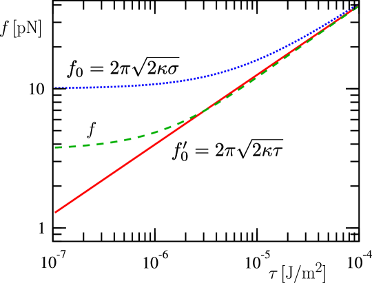
Refer to caption

Figure 5.10: Average force f𝑓f as a function of the effectively applied mechanical tension τ𝜏\tau. The red solid line shows the usual relation given in eq.(5.69), under the assumption that τσ𝜏𝜎\tau\approx\sigma and neglecting thermal fluctuations. The upper blue dotted line shown the expected relation if one considers τ=σσ0𝜏𝜎subscript𝜎0\tau=\sigma-\sigma_{0}, but neglects the thermal fluctuations (eq.(5.71)). Finally, the green dashed curve represents the expected relation taking into account both the difference between τ𝜏\tau and σ𝜎\sigma and the thermal fluctuations (eq.(5.72)). The parameters used are Λa=1Λ𝑎1\Lambda a=1 with a5nmsimilar-to-or-equals𝑎5nma\simeq 5\,\mathrm{nm}, kBT4×1021Jsimilar-to-or-equalssubscript𝑘𝐵𝑇4superscript1021Jk_{B}T\simeq 4\times 10^{-21}\,\mathrm{J} and κ50kBTsimilar-to-or-equals𝜅50subscript𝑘𝐵𝑇\kappa\simeq 50\,k_{B}T.

We observe that thermal fluctuations are indeed important: the average force f𝑓f differs significantly from the mean-field approximation f0=2π2κσsubscript𝑓02𝜋2𝜅𝜎f_{0}=2\pi\sqrt{2\kappa\sigma}. The relative error (f0f)/fsubscript𝑓0𝑓𝑓(f_{0}-f)/f is of order 5%percent55\% at τ=104J/m2𝜏superscript104Jsuperscriptm2\tau=10^{-4}\,\mathrm{J/m}^{2}, of 30%percent3030\% at τ=105J/m2𝜏superscript105Jsuperscriptm2\tau=10^{-5}\,\mathrm{J/m}^{2} and it reaches 100%percent100100\% at τ=106J/m2𝜏superscript106Jsuperscriptm2\tau=10^{-6}\,\mathrm{J/m}^{2} (see Fig. 5.10). Interestingly, the relative error (f0f)/fsuperscriptsubscript𝑓0𝑓𝑓(f_{0}^{\prime}-f)/f is much smaller than (f0f)/fsubscript𝑓0𝑓𝑓(f_{0}-f)/f (see Fig. 5.10). Indeed, it is less than 1%percent11\% for τ>105J/m2𝜏superscript105Jsuperscriptm2\tau>10^{-5}\,\mathrm{J/m}^{2}, and it becomes larger than 20%percent2020\% only for τ<106J/m2𝜏superscript106Jsuperscriptm2\tau<10^{-6}\,\mathrm{J/m}^{2}. Hence f0subscriptsuperscript𝑓0f^{\prime}_{0} appears to be indeed a good approximation of the average force: for τ>106J/m2𝜏superscript106Jsuperscriptm2\tau>10^{-6}\,\mathrm{J/m}^{2}, one should expect a linear behavior. This happens however by a happy coincidence, since one makes two non justified assumptions.

Let us discuss what could be done experimentally in order to test these predictions. The difference between f𝑓f and f0superscriptsubscript𝑓0f_{0}^{\prime} will be difficult to evidence, because one should detect a difference of the order of a few pNpN\mathrm{pN} while measuring precisely the tension in the range τ<106J/m2𝜏superscript106Jsuperscriptm2\tau<10^{-6}\,\mathrm{J/m}^{2}. It should be easier to detect the difference between f𝑓f and f0=2π2κσsubscript𝑓02𝜋2𝜅𝜎f_{0}=2\pi\sqrt{2\kappa\sigma}, since it is already significant at τ105J/m2similar-to-or-equals𝜏superscript105Jsuperscriptm2\tau\simeq 10^{-5}\,\mathrm{J/m}^{2}. This could be done if the tension r𝑟r were measured simultaneously from the thermal fluctuation spectrum of the vesicle from which the tubule is drawn and then assuming that rσ𝑟𝜎r\approx\sigma. It would be interesting to measure R0subscript𝑅0R_{0} as a function of τ𝜏\tau directly, in order to check the difference between R0subscript𝑅0R_{0} and the usually assumed relation κ/(2τ)𝜅2𝜏\sqrt{\kappa/(2\tau)} (we expect κ/[2(τ+σ0)]𝜅delimited-[]2𝜏subscript𝜎0\sqrt{\kappa/[2(\tau+\sigma_{0})]}). This would require a specific experiment, since R0subscript𝑅0R_{0} is normally below optical resolution.

5.5 In a nutshell

The mean-field force needed to extract a membrane nanotube in terms of the membrane rigidity κ𝜅\kappa and it’s microscopical tension σ𝜎\sigma is well known and given by

f0=2π2κσ.subscript𝑓02𝜋2𝜅𝜎f_{0}=2\pi\sqrt{2\kappa\sigma}\,. (5.73)

Assuming that thermal fluctuations are negligible and that the mechanical tension τ𝜏\tau coming from the flattening of the membrane’s fluctuation is a good approximation for σ𝜎\sigma, this relation seemed to be successfully experimentally verified. Recently, however, it was shown that these nanotubes, due to their geometry, present very soft modes and should thus have strong fluctuations, implying that the actual force f𝑓f needed to extract a tube should be somewhat different from f0subscript𝑓0f_{0}. To evaluate this difference, we have derived the stress tensor for quasi-cylindrical geometry and averaged it appropriately, yielding

ff0[12πσ0σ],similar-to-or-equals𝑓subscript𝑓0delimited-[]12𝜋subscript𝜎0𝜎f\simeq f_{0}\left[1-\frac{2}{\pi}\,\frac{\sigma_{0}}{\sigma}\right]\,, (5.74)

where

σ0=κΛ28πκβ.subscript𝜎0𝜅superscriptΛ28𝜋𝜅𝛽\sigma_{0}=\frac{\kappa\Lambda^{2}}{8\pi\kappa\beta}\,. (5.75)

Numerically, the difference between f𝑓f and f0subscript𝑓0f_{0} is non-negligible. The fact that it has not been previously noticed comes from a happy coincidence: the assumption that στ𝜎𝜏\sigma\approx\tau seems to make up for the neglected thermal fluctuations.

Chapter 6 Fluctuation of the force needed to extract a membrane nanotube

As discussed in section 1.4.4, nanotubes are extracted from vesicles by applying point forces. In the last chapter, we have described a popular method for pulling nanotubes, which consists in attaching a glass bead to the membrane and displacing the bead with a laser. The advantage of this method is that one deduces with precision the applied force by measuring the position of the center of the beam and the position of the bead along the tube’s axis (see Fig. 5.1). In general, only the force in the direction of the tube’s axis fzsubscript𝑓𝑧f_{z} is measured, since by symmetry the averages of the transversal components of the force vanish. A typical time-sequence of the bead’s position along the tube’s axis and force fzsubscript𝑓𝑧f_{z} can be seen in Fig. 6.1.

Refer to caption
Figure 6.1: Extraction and retraction of a nanotube using a glass bead and an optical trap [120]. The blue well-defined line represents the displacement of the glass bead as a function of time. The bead was moved in order to elongate the vesicle and create a tube (from 00 up to 80s80s80\,\mathrm{s}), then kept roughly at the same point for 20s20s20\,\mathrm{s} and finally moved in the opposite direction. The red fluctuating line shows the force applied to the bead. Note that there is a force barrier to form a tube (region before 40s40s40\,\mathrm{s}), but afterwards, the force does almost not depend on the length of the tube.

In the last chapter and here, we are interested in the situation where the tube’s length is kept constant (results published in [6]). In Fig. 6.1, this corresponds to the interval between the dashed lines, where we can see that the force is roughly a plateau. We have studied the average value of this plateau in the last chapter, obtaining

fz2π2κσ[1kBT4π2Λ2σ],similar-to-or-equalsdelimited-⟨⟩subscript𝑓𝑧2𝜋2𝜅𝜎delimited-[]1subscript𝑘B𝑇4superscript𝜋2superscriptΛ2𝜎\langle f_{z}\rangle\simeq 2\pi\sqrt{2\kappa\sigma}\left[1-\frac{k_{\mathrm{B}}T}{4\pi^{2}}\,\frac{\Lambda^{2}}{\sigma}\right]\,, (6.1)

where κ𝜅\kappa is the bending rigidity, ΛΛ\Lambda is a wave-vector cutoff and σ𝜎\sigma is the tension associated to the microscopical area of the membrane.

Interestingly, in Fig. 6.1, we see that the measures of fzsubscript𝑓𝑧f_{z} present a considerable dispersion, mainly coming from the fluctuations of the bead’s position (we cannot see this fluctuation on the blue curve due to the length scale). In effect, the bead is subjected to many sources of thermal fluctuations, such as the fluctuating forces that the solvent applies to the bead, producing a Brownian movement, and the thermal fluctuations of the membrane to which the bead is attached.

As membrane nanotubes present very soft Goldstone modes [7], the membrane fluctuation is possibly responsible for an important part of the dispersion, in which case measures of force fluctuation could be used to characterize membranes. Indeed, in section 1.4.4, we have seen that from measures of the average force fzdelimited-⟨⟩subscript𝑓𝑧\langle f_{z}\rangle, one can deduce the bending rigidity of a membrane. Likewise, the fluctuation of the force in the direction of the tube’s axis, easily accessible with the same experimental setting, could provide supplemental informations. Accordingly, our aim in this chapter is to study the contribution of the membrane fluctuations to the fluctuation of the force in the direction of the tube’s axis, defined through

(Δfz)2superscriptΔsubscript𝑓𝑧2\displaystyle(\Delta f_{z})^{2} =\displaystyle= fz2fz2.delimited-⟨⟩superscriptsubscript𝑓𝑧2superscriptdelimited-⟨⟩subscript𝑓𝑧2\displaystyle\langle f_{z}^{2}\rangle-\langle f_{z}\rangle^{2}\,. (6.2)

As in chapter 5, we will consider a tube small enough so that we can consider the vesicle from which it is extracted as a lipid reservoir and we can neglect volume constraints. In section 6.1 we remind some important results deduced in the last chapter. To evaluate ΔfzΔsubscript𝑓𝑧\Delta f_{z}, we will use the diagrammatic tools introduced in chapter 3. We will thus sum-up some properties of these diagrams and write the stress tensor using them in section 6.2. In section 6.3, we evaluate ΔfzΔsubscript𝑓𝑧\Delta f_{z}. Finally, we discuss our results in section 6.4.

6.1 Some important definitions and results

As in chapter 5, we shall restrict our attention to deformed tubes weakly departing from the mean-field cylinder, whose radius is given by

R0=κ2σ.subscript𝑅0𝜅2𝜎R_{0}=\sqrt{\frac{\kappa}{2\sigma}}\,. (6.3)

We will keep the same coordinate system presented in Fig. 5.3 and the tube’s shape will be parametrized by eq.(5.5).

As before, we consider a tube relatively short compared to the vesicle from which it is extracted, so that the vesicle can be treated as a lipid reservoir. In the case of short tubes, one can also neglect the pressure difference across the tube’s membrane (see discussion in section 5.1). The energy is simply given by the Helfrich Hamiltonian, given in eq.(5.8) and eq.(5.9). The corresponding correlation function is given by

G(ρρ,zz)𝐺𝜌superscript𝜌𝑧superscript𝑧\displaystyle G(\rho-\rho^{\prime},z-z^{\prime}) =\displaystyle= u(ρ,z)u(ρ,z),delimited-⟨⟩𝑢𝜌𝑧𝑢superscript𝜌superscript𝑧\displaystyle\langle u(\rho,z)\,u(\rho^{\prime},z^{\prime})\rangle\,, (6.4)
=\displaystyle= kBTR02πκLmq¯eiR0[m(ρρ)+q¯(zz)](m21)2+q¯2(q¯2+2m2),subscript𝑘B𝑇subscript𝑅02𝜋𝜅𝐿subscript𝑚subscript¯𝑞superscript𝑒𝑖subscript𝑅0delimited-[]𝑚𝜌superscript𝜌¯𝑞𝑧superscript𝑧superscriptsuperscript𝑚212superscript¯𝑞2superscript¯𝑞22superscript𝑚2\displaystyle\frac{k_{\mathrm{B}}T\,R_{0}}{2\pi\kappa L}\sum_{m}\sum_{\bar{q}}\frac{e^{\frac{i}{R_{0}}\left[m(\rho-\rho^{\prime})+\bar{q}(z-z^{\prime})\right]}}{(m^{2}-1)^{2}+\bar{q}^{2}(\bar{q}^{2}+2m^{2})}\,,

where m{M,,M}𝑚𝑀𝑀m\in\{-M,\cdots,M\} and q¯=2πnR0/L¯𝑞2𝜋𝑛subscript𝑅0𝐿\bar{q}=2\pi nR_{0}/L, with n{N,,N}𝑛𝑁𝑁n\in\{-N,\cdots,N\}. We remind that the upper bounds N𝑁N and M𝑀M are given by M=ΛR0𝑀Λsubscript𝑅0M=\Lambda R_{0} and q¯max=2πNR0/L=ΛR0subscript¯𝑞max2𝜋𝑁subscript𝑅0𝐿Λsubscript𝑅0\bar{q}_{\mathrm{max}}=2\pi NR_{0}/L=\Lambda R_{0}, where Λ=1/aΛ1𝑎\Lambda=1/a is the high wave-vector cutoff and a𝑎a is of the order of the membrane thickness.

The force needed to extract a tube is given by

𝒇=(02πR0Σrz𝑑ρ)𝒆r+(02πR0Σρz𝑑ρ)𝒆ρ+(02πR0Σzz𝑑ρ)𝒆z,𝒇superscriptsubscript02𝜋subscript𝑅0subscriptΣ𝑟𝑧differential-d𝜌subscript𝒆𝑟superscriptsubscript02𝜋subscript𝑅0subscriptΣ𝜌𝑧differential-d𝜌subscript𝒆𝜌superscriptsubscript02𝜋subscript𝑅0subscriptΣ𝑧𝑧differential-d𝜌subscript𝒆𝑧\bm{f}=\left(\int_{0}^{2\pi R_{0}}\Sigma_{rz}\,d\rho\right)\bm{e}_{r}+\left(\int_{0}^{2\pi R_{0}}\Sigma_{\rho z}\,d\rho\right)\bm{e}_{\rho}+\left(\int_{0}^{2\pi R_{0}}\Sigma_{zz}\,d\rho\right)\bm{e}_{z}\,, (6.5)

where ΣrzsubscriptΣ𝑟𝑧\Sigma_{rz}, ΣρzsubscriptΣ𝜌𝑧\Sigma_{\rho z} and

ΣzzsubscriptΣ𝑧𝑧\displaystyle\Sigma_{zz} =\displaystyle= σ{2+u2+2R02[uρ2+(2u1)uρρ]\displaystyle\sigma\left\{2+u^{2}+2R_{0}^{2}\left[u_{\rho}^{2}+\left(2u-1\right)u_{\rho\rho}\right]\right. (6.6)
+\displaystyle+ R04[uρρ2uzz2+2uz(uzzz+uρρz)]}\displaystyle R_{0}^{4}\left.\left[u_{\rho\rho}^{2}-u_{zz}^{2}+2u_{z}\left(u_{zzz}+u_{\rho\rho z}\right)\right]\right\}

are the components of the projected stress tensor for quasi-cylindrical geometry derived in section 5.2. As in the last chapter, the subscript ρ𝜌\rho (resp. z𝑧z) indicates the derivative with respect to ρ𝜌\rho (resp. z𝑧z). Here we will evaluate the fluctuation of the force in the direction of the tube’s axis:

(Δfz)2superscriptΔsubscript𝑓𝑧2\displaystyle(\Delta f_{z})^{2} =\displaystyle= fz2fz2,delimited-⟨⟩superscriptsubscript𝑓𝑧2superscriptdelimited-⟨⟩subscript𝑓𝑧2\displaystyle\langle f_{z}^{2}\rangle-\langle f_{z}\rangle^{2}\,, (6.7)
=\displaystyle= 02πR002πR0Σzz(ρ,z)Σzz(ρ,z)Σzz2dρdρ.superscriptsubscript02𝜋subscript𝑅0superscriptsubscript02𝜋subscript𝑅0delimited-⟨⟩subscriptΣ𝑧𝑧𝜌𝑧subscriptΣ𝑧𝑧superscript𝜌𝑧superscriptdelimited-⟨⟩subscriptΣ𝑧𝑧2𝑑𝜌𝑑superscript𝜌\displaystyle\int_{0}^{2\pi R_{0}}\int_{0}^{2\pi R_{0}}\langle\Sigma_{zz}(\rho,z)\Sigma_{zz}(\rho^{\prime},z)\rangle-\langle\Sigma_{zz}\rangle^{2}\,d\rho d\rho^{\prime}\,.

As in chapter 3, the first step is to evaluate the correlation function of the stress tensor over the same section of tube:

C(ρ,ρ)=Σzz(ρ,z)Σzz(ρ,z)Σzz2.𝐶𝜌superscript𝜌delimited-⟨⟩subscriptΣ𝑧𝑧𝜌𝑧subscriptΣ𝑧𝑧superscript𝜌𝑧superscriptdelimited-⟨⟩subscriptΣ𝑧𝑧2C(\rho,\rho^{\prime})=\langle\Sigma_{zz}(\rho,z)\Sigma_{zz}(\rho^{\prime},z)\rangle-\langle\Sigma_{zz}\rangle^{2}\,. (6.8)

To do so, we will use another time the diagrammatic tools introduced in chapter 3. We recall their properties in the next section.

6.2 Diagrammatic tools

Throughout this chapter, we will use notations similar to those introduced in section 3.2. Each field u(ρ,z)𝑢𝜌𝑧u(\rho,z) is represented by a straight line. The derivatives with respect to ρ𝜌\rho are represented by a dot over the field, while a derivative with respect to z𝑧z is represented by a slash. An adapted diagrammatic vocabulary is presented in table 6.1.

Usually Diagrammatically
u(ρ,z)𝑢𝜌𝑧u(\rho,z)
[Uncaptioned image]
uz(ρ,z)subscript𝑢𝑧𝜌𝑧u_{z}(\rho,z)
[Uncaptioned image]
uρ(ρ,z)subscript𝑢𝜌𝜌𝑧u_{\rho}(\rho,z)
[Uncaptioned image]
u(ρ,z)u(ρ,z)𝑢𝜌𝑧𝑢𝜌𝑧u(\rho,z)\,u(\rho,z)
[Uncaptioned image]
u(ρ,z)u(ρ,z)𝑢𝜌𝑧𝑢superscript𝜌superscript𝑧u(\rho,z)\,u(\rho^{\prime},z^{\prime})
[Uncaptioned image]
[Uncaptioned image]
Table 6.1: Basic translation rules from the usual notation into diagrams.

Averages are performed using Wick’s theorem, i. e., by adding all complete contractions of fields. Each contraction yields a propagator and, as in the case of section 3.2, one can pass a derivative from one branch of the propagator to the other by multiplying the diagram’s coefficient by 11-1. For instance, with 𝒓=(ρ,z)𝒓𝜌𝑧\bm{r}=(\rho,z) and 𝒓=(ρ,z)superscript𝒓superscript𝜌superscript𝑧\bm{r}^{\prime}=(\rho^{\prime},z^{\prime}), we have

[Uncaptioned image]𝒓[Uncaptioned image]𝒓delimited-⟨⟩[Uncaptioned image]𝒓[Uncaptioned image]superscript𝒓bold-′\displaystyle\left\langle\begin{array}[]{c}\begin{tabular}[]{c}\includegraphics[angle={0},scale={.18}]{./figures_Chap4/simple_1.epsi}\end{tabular}\\ {}^{\bm{r}}\end{array}\begin{array}[]{c}\begin{tabular}[]{c}\includegraphics[angle={0},scale={.18}]{./figures_Chap4/simple_4.epsi}\end{tabular}\\ {}^{\bm{r^{\prime}}}\end{array}\right\rangle =\displaystyle= [Uncaptioned image],[Uncaptioned image]\displaystyle\begin{tabular}[]{c}\includegraphics[angle={0},scale={.18}]{./figures_Chap4/reto_3.epsi}\end{tabular}\,, (6.16)
=\displaystyle= (1)×[Uncaptioned image],1[Uncaptioned image]\displaystyle(-1)\times\begin{tabular}[]{c}\includegraphics[angle={0},scale={.18}]{./figures_Chap4/reto_4.epsi}\end{tabular}\,,
=\displaystyle= (1)×zρ[G(𝒓𝒓)],1subscript𝑧subscript𝜌delimited-[]𝐺superscript𝒓𝒓\displaystyle(-1)\times\partial_{z}\partial_{\rho}\,[G(\bm{r}^{\prime}-\bm{r})]\,,
=\displaystyle= kBTR02πκLmq¯(im/R0)(iq¯/R0)eiR0[m(ρρ)+q¯(zz)](m21)2+q¯2(q¯2+2m2).subscript𝑘B𝑇subscript𝑅02𝜋𝜅𝐿subscript𝑚subscript¯𝑞𝑖𝑚subscript𝑅0𝑖¯𝑞subscript𝑅0superscript𝑒𝑖subscript𝑅0delimited-[]𝑚𝜌superscript𝜌¯𝑞𝑧superscript𝑧superscriptsuperscript𝑚212superscript¯𝑞2superscript¯𝑞22superscript𝑚2\displaystyle\frac{k_{\mathrm{B}}T\,R_{0}}{2\pi\kappa L}\sum_{m}\sum_{\bar{q}}\frac{(i\,m/R_{0})(i\,\bar{q}/R_{0})\,e^{\frac{i}{R_{0}}\left[m(\rho-\rho^{\prime})+\bar{q}(z-z^{\prime})\right]}}{(m^{2}-1)^{2}+\bar{q}^{2}(\bar{q}^{2}+2m^{2})}\,. (6.19)

This time, once the derivatives are grouped, every slash contributes with a factor iq¯/R0𝑖¯𝑞subscript𝑅0i\,\bar{q}/R_{0} and every dot contributes with a factor im/R0𝑖𝑚subscript𝑅0i\,m/R_{0}.

In the following section, we will evaluate the propagators between points over the same section of tube, i. e., with z=z𝑧superscript𝑧z=z^{\prime}. In this case, as the sum over q¯¯𝑞\bar{q} is symmetrical, an uneven number of slashes over a propagator implies a vanishing contribution. Here follows a typical example of the terms that we will need to evaluate:

[Uncaptioned image]𝒓[Uncaptioned image]𝒓delimited-⟨⟩[Uncaptioned image]𝒓[Uncaptioned image]superscript𝒓\displaystyle\left\langle\begin{array}[]{c}\begin{tabular}[]{c}\includegraphics[angle={0},scale={.18}]{./figures_Chap4/champ_7_n1.epsi}\end{tabular}\\ {}^{\bm{r}}\end{array}\begin{array}[]{c}\begin{tabular}[]{c}\includegraphics[angle={0},scale={.18}]{./figures_Chap4/champ_7_n2.epsi}\end{tabular}\\ {}^{\bm{r}^{\prime}}\end{array}\right\rangle =\displaystyle= [Uncaptioned image]𝒓[Uncaptioned image]𝒓+[Uncaptioned image]+[Uncaptioned image],[Uncaptioned image]𝒓[Uncaptioned image]superscript𝒓[Uncaptioned image][Uncaptioned image]\displaystyle\begin{array}[]{c}\begin{tabular}[]{c}\includegraphics[angle={0},scale={.18}]{./figures_Chap4/wick_n1.epsi}\end{tabular}\\ {}^{\bm{r}}\end{array}\begin{array}[]{c}\begin{tabular}[]{c}\includegraphics[angle={0},scale={.18}]{./figures_Chap4/wick_n2.epsi}\end{tabular}\\ {}^{\bm{r}^{\prime}}\end{array}+\begin{tabular}[]{c}\includegraphics[angle={0},scale={.18}]{./figures_Chap4/peixe_n11.epsi}\end{tabular}+\begin{tabular}[]{c}\includegraphics[angle={0},scale={.18}]{./figures_Chap4/peixe_n21.epsi}\end{tabular}\,, (6.34)
=\displaystyle=
[Uncaptioned image]
[Uncaptioned image]
+[Uncaptioned image]+[Uncaptioned image]
,
[Uncaptioned image]
[Uncaptioned image]
[Uncaptioned image][Uncaptioned image]
\displaystyle\begin{tabular}[]{c}\includegraphics[angle={0},scale={.18}]{./figures_Chap4/wick_n1_1.epsi}\end{tabular}\begin{tabular}[]{c}\includegraphics[angle={0},scale={.18}]{./figures_Chap4/wick_n1_1.epsi}\end{tabular}+\begin{tabular}[]{c}\includegraphics[angle={0},scale={.18}]{./figures_Chap4/peixe_n1_1.epsi}\end{tabular}+\begin{tabular}[]{c}\includegraphics[angle={0},scale={.18}]{./figures_Chap4/peixe_n2_1.epsi}\end{tabular}\,,
(6.39)

which one can readily read by noting the equivalence

[Uncaptioned image]=[Uncaptioned image]×[Uncaptioned image].[Uncaptioned image][Uncaptioned image][Uncaptioned image]\begin{tabular}[]{c}\includegraphics[angle={0},scale={.18}]{./figures_Chap4/peixe_n2_1.epsi}\end{tabular}=\begin{tabular}[]{c}\includegraphics[angle={0},scale={.18}]{./figures_Chap4/reto_4.epsi}\end{tabular}\times\begin{tabular}[]{c}\includegraphics[angle={0},scale={.18}]{./figures_Chap4/reto_4.epsi}\end{tabular}\,. (6.41)

As the number of slashes over these propagators is uneven, the contribution of this diagram vanishes. The first term of eq.(LABEL:eq_4_avediag) is also composed by diagrams with an uneven number of slashes whose contribution vanishes. At the end, one obtains simply

[Uncaptioned image]𝒓[Uncaptioned image]𝒓delimited-⟨⟩[Uncaptioned image]𝒓[Uncaptioned image]superscript𝒓\displaystyle\left\langle\begin{array}[]{c}\begin{tabular}[]{c}\includegraphics[angle={0},scale={.18}]{./figures_Chap4/champ_7_n1.epsi}\end{tabular}\\ {}^{\bm{r}}\end{array}\begin{array}[]{c}\begin{tabular}[]{c}\includegraphics[angle={0},scale={.18}]{./figures_Chap4/champ_7_n2.epsi}\end{tabular}\\ {}^{\bm{r}^{\prime}}\end{array}\right\rangle =\displaystyle= [Uncaptioned image].[Uncaptioned image]\displaystyle\begin{tabular}[]{c}\includegraphics[angle={0},scale={.18}]{./figures_Chap4/peixe_n1_1.epsi}\end{tabular}\,. (6.49)

In the next section, we will re-derive Σzzdelimited-⟨⟩subscriptΣ𝑧𝑧\langle\Sigma_{zz}\rangle in terms of diagrams in order to gain familiarity with these tools.

6.2.1 Getting familiar: re-deriving 𝚺𝒛𝒛delimited-⟨⟩subscript𝚺𝒛𝒛\bm{\langle\Sigma_{zz}\rangle}

The component ΣzzsubscriptΣ𝑧𝑧\Sigma_{zz}, given in eq.(6.6), can be written in terms of diagrams as

σ1Σzzsuperscript𝜎1delimited-⟨⟩subscriptΣ𝑧𝑧\displaystyle\sigma^{-1}\,\langle\Sigma_{zz}\rangle =\displaystyle= 2+[Uncaptioned image]+2R02[Uncaptioned image]+4R02[Uncaptioned image]2R02[Uncaptioned image]2[Uncaptioned image]2superscriptsubscript𝑅02[Uncaptioned image]4superscriptsubscript𝑅02[Uncaptioned image]2superscriptsubscript𝑅02[Uncaptioned image]\displaystyle 2+\begin{tabular}[]{c}\includegraphics[angle={0},scale={.18}]{./figures_Chap4/champ_0.epsi}\end{tabular}+2R_{0}^{2}\begin{tabular}[]{c}\includegraphics[angle={0},scale={.18}]{./figures_Chap4/champ_4.epsi}\end{tabular}+4R_{0}^{2}\begin{tabular}[]{c}\includegraphics[angle={0},scale={.18}]{./figures_Chap4/champ_12.epsi}\end{tabular}-2R_{0}^{2}\begin{tabular}[]{c}\includegraphics[angle={0},scale={.18}]{./figures_Chap4/simple_5.epsi}\end{tabular} (6.54)
+\displaystyle+ R04[Uncaptioned image]R04[Uncaptioned image]+2R04[Uncaptioned image]+2R04[Uncaptioned image].superscriptsubscript𝑅04[Uncaptioned image]superscriptsubscript𝑅04[Uncaptioned image]2superscriptsubscript𝑅04[Uncaptioned image]2superscriptsubscript𝑅04[Uncaptioned image]\displaystyle R_{0}^{4}\begin{tabular}[]{c}\includegraphics[angle={0},scale={.18}]{./figures_Chap4/champ_6.epsi}\end{tabular}-R_{0}^{4}\begin{tabular}[]{c}\includegraphics[angle={0},scale={.18}]{./figures_Chap4/champ_5.epsi}\end{tabular}+2R_{0}^{4}\begin{tabular}[]{c}\includegraphics[angle={0},scale={.18}]{./figures_Chap4/champ_1.epsi}\end{tabular}+2R_{0}^{4}\begin{tabular}[]{c}\includegraphics[angle={0},scale={.18}]{./figures_Chap4/champ_2.epsi}\end{tabular}\,. (6.59)

Using Wick’s theorem to evaluate the average, we obtain

σ1Σzzsuperscript𝜎1delimited-⟨⟩subscriptΣ𝑧𝑧\displaystyle\sigma^{-1}\,\langle\Sigma_{zz}\rangle =\displaystyle= 2+[Uncaptioned image]+2R02[Uncaptioned image]+4R02[Uncaptioned image]2[Uncaptioned image]2superscriptsubscript𝑅02[Uncaptioned image]4superscriptsubscript𝑅02[Uncaptioned image]\displaystyle 2+\begin{tabular}[]{c}\includegraphics[angle={0},scale={.18}]{./figures_Chap4/wick_0.epsi}\end{tabular}+2R_{0}^{2}\begin{tabular}[]{c}\includegraphics[angle={0},scale={.18}]{./figures_Chap4/wick_3.epsi}\end{tabular}+4R_{0}^{2}\begin{tabular}[]{c}\includegraphics[angle={0},scale={.18}]{./figures_Chap4/wick_14.epsi}\end{tabular} (6.63)
+\displaystyle+ R04[Uncaptioned image]R04[Uncaptioned image]+2R04[Uncaptioned image]+2R04[Uncaptioned image].superscriptsubscript𝑅04[Uncaptioned image]superscriptsubscript𝑅04[Uncaptioned image]2superscriptsubscript𝑅04[Uncaptioned image]2superscriptsubscript𝑅04[Uncaptioned image]\displaystyle R_{0}^{4}\begin{tabular}[]{c}\includegraphics[angle={0},scale={.18}]{./figures_Chap4/wick_5.epsi}\end{tabular}-R_{0}^{4}\begin{tabular}[]{c}\includegraphics[angle={0},scale={.18}]{./figures_Chap4/wick_6.epsi}\end{tabular}+2R_{0}^{4}\begin{tabular}[]{c}\includegraphics[angle={0},scale={.18}]{./figures_Chap4/wick_1.epsi}\end{tabular}+2R_{0}^{4}\begin{tabular}[]{c}\includegraphics[angle={0},scale={.18}]{./figures_Chap4/wick_15.epsi}\end{tabular}\,. (6.68)

Grouping the derivatives, we have

σ1Σzzsuperscript𝜎1delimited-⟨⟩subscriptΣ𝑧𝑧\displaystyle\sigma^{-1}\,\langle\Sigma_{zz}\rangle =\displaystyle= 2+[Uncaptioned image]2R02[Uncaptioned image]+4R02[Uncaptioned image]2[Uncaptioned image]2superscriptsubscript𝑅02[Uncaptioned image]4superscriptsubscript𝑅02[Uncaptioned image]\displaystyle 2+\begin{tabular}[]{c}\includegraphics[angle={0},scale={.18}]{./figures_Chap4/wick_0_0.epsi}\end{tabular}-2R_{0}^{2}\begin{tabular}[]{c}\includegraphics[angle={0},scale={.18}]{./figures_Chap4/wick_7.epsi}\end{tabular}+4R_{0}^{2}\begin{tabular}[]{c}\includegraphics[angle={0},scale={.18}]{./figures_Chap4/wick_7.epsi}\end{tabular} (6.72)
+\displaystyle+ R04[Uncaptioned image]R04[Uncaptioned image]2R04[Uncaptioned image]2R04[Uncaptioned image],superscriptsubscript𝑅04[Uncaptioned image]superscriptsubscript𝑅04[Uncaptioned image]2superscriptsubscript𝑅04[Uncaptioned image]2superscriptsubscript𝑅04[Uncaptioned image]\displaystyle R_{0}^{4}\begin{tabular}[]{c}\includegraphics[angle={0},scale={.18}]{./figures_Chap4/wick_9.epsi}\end{tabular}-R_{0}^{4}\begin{tabular}[]{c}\includegraphics[angle={0},scale={.18}]{./figures_Chap4/wick_10.epsi}\end{tabular}-2R_{0}^{4}\begin{tabular}[]{c}\includegraphics[angle={0},scale={.18}]{./figures_Chap4/wick_10.epsi}\end{tabular}-2R_{0}^{4}\begin{tabular}[]{c}\includegraphics[angle={0},scale={.18}]{./figures_Chap4/wick_11.epsi}\end{tabular}\,, (6.77)
=\displaystyle= 2+[Uncaptioned image]+2R02[Uncaptioned image]+R04[Uncaptioned image]3R04[Uncaptioned image]2R04[Uncaptioned image].2[Uncaptioned image]2superscriptsubscript𝑅02[Uncaptioned image]superscriptsubscript𝑅04[Uncaptioned image]3superscriptsubscript𝑅04[Uncaptioned image]2superscriptsubscript𝑅04[Uncaptioned image]\displaystyle 2+\begin{tabular}[]{c}\includegraphics[angle={0},scale={.18}]{./figures_Chap4/wick_0_0.epsi}\end{tabular}+2R_{0}^{2}\begin{tabular}[]{c}\includegraphics[angle={0},scale={.18}]{./figures_Chap4/wick_7.epsi}\end{tabular}+R_{0}^{4}\begin{tabular}[]{c}\includegraphics[angle={0},scale={.18}]{./figures_Chap4/wick_9.epsi}\end{tabular}-3R_{0}^{4}\begin{tabular}[]{c}\includegraphics[angle={0},scale={.18}]{./figures_Chap4/wick_10.epsi}\end{tabular}-2R_{0}^{4}\begin{tabular}[]{c}\includegraphics[angle={0},scale={.18}]{./figures_Chap4/wick_11.epsi}\end{tabular}\,. (6.83)

Let’s read eq.(LABEL:eq_4_aveSigma):

Σzzdelimited-⟨⟩subscriptΣ𝑧𝑧\displaystyle\langle\Sigma_{zz}\rangle =\displaystyle= 2σ+σkBTR02πκLmq¯1+2(im)2+(im)43(iq¯)42(im)2(iq¯)2(m21)2+q¯2(q¯2+2m2),2𝜎𝜎subscript𝑘B𝑇subscript𝑅02𝜋𝜅𝐿subscript𝑚subscript¯𝑞12superscript𝑖𝑚2superscript𝑖𝑚43superscript𝑖¯𝑞42superscript𝑖𝑚2superscript𝑖¯𝑞2superscriptsuperscript𝑚212superscript¯𝑞2superscript¯𝑞22superscript𝑚2\displaystyle 2\sigma+\sigma\frac{k_{\mathrm{B}}T\,R_{0}}{2\pi\kappa L}\sum_{m}\sum_{\bar{q}}\frac{1+2(i\,m)^{2}+(i\,m)^{4}-3(i\,\bar{q})^{4}-2(i\,m)^{2}(i\,\bar{q})^{2}}{(m^{2}-1)^{2}+\bar{q}^{2}(\bar{q}^{2}+2m^{2})}\,, (6.85)
=\displaystyle= 2σ+kBT4πR0Lmq¯(1m2)2q¯2(3q¯2+2m2)(m21)2+q¯2(q¯2+2m2),2𝜎subscript𝑘B𝑇4𝜋subscript𝑅0𝐿subscript𝑚subscript¯𝑞superscript1superscript𝑚22superscript¯𝑞23superscript¯𝑞22superscript𝑚2superscriptsuperscript𝑚212superscript¯𝑞2superscript¯𝑞22superscript𝑚2\displaystyle 2\sigma+\frac{k_{\mathrm{B}}T}{4\pi R_{0}L}\sum_{m}\sum_{\bar{q}}\frac{(1-m^{2})^{2}-\bar{q}^{2}(3\bar{q}^{2}+2m^{2})}{(m^{2}-1)^{2}+\bar{q}^{2}(\bar{q}^{2}+2m^{2})}\,,

which coincides, as it should, with eq.(5.61).

6.3 Evaluation of the fluctuation of the force

Aiming to obtain ΔfzΔsubscript𝑓𝑧\Delta f_{z}, we start this section by evaluating the correlation function of the component ΣzzsubscriptΣ𝑧𝑧\Sigma_{zz} of the stress tensor. In section 6.3.2, we integrate twice this correlation and derive the force fluctuation. There, we discuss also some approximations in order to obtain a simple analytical expression. Finally, we conclude by a short discussion on the validity of our final result in section 6.3.3.

6.3.1 Correlation of 𝚺𝒛𝒛subscript𝚺𝒛𝒛\bm{\Sigma_{zz}}

Here we will evaluate the correlation function

C(ρ,ρ)=Σzz(ρ,z)Σzz(ρ,z)Σzz2.𝐶𝜌superscript𝜌delimited-⟨⟩subscriptΣ𝑧𝑧𝜌𝑧subscriptΣ𝑧𝑧superscript𝜌𝑧superscriptdelimited-⟨⟩subscriptΣ𝑧𝑧2C(\rho,\rho^{\prime})=\langle\Sigma_{zz}(\rho,z)\Sigma_{zz}(\rho^{\prime},z)\rangle-\langle\Sigma_{zz}\rangle^{2}\,. (6.86)

From eq.(6.59), using Wick’s Theorem and the rules presented in section 6.2, we obtain

σ2C(ρ,ρ)superscript𝜎2𝐶𝜌superscript𝜌\displaystyle\sigma^{-2}\,C(\rho,\rho^{\prime}) =\displaystyle= 2[Uncaptioned image]+8R02[Uncaptioned image]+16R02[Uncaptioned image]+28R04[Uncaptioned image]2[Uncaptioned image]8superscriptsubscript𝑅02[Uncaptioned image]16superscriptsubscript𝑅02[Uncaptioned image]28superscriptsubscript𝑅04[Uncaptioned image]\displaystyle 2\begin{tabular}[]{c}\includegraphics[angle={0},scale={.5}]{./figures_Chap4/diag.eps}\end{tabular}+8R_{0}^{2}\begin{tabular}[]{c}\includegraphics[angle={0},scale={.5}]{./figures_Chap4/diagpop.eps}\end{tabular}+16R_{0}^{2}\begin{tabular}[]{c}\includegraphics[angle={0},scale={.5}]{./figures_Chap4/diagppo.eps}\end{tabular}+28R_{0}^{4}\begin{tabular}[]{c}\includegraphics[angle={0},scale={.5}]{./figures_Chap4/diagppopp.eps}\end{tabular} (6.91)
+\displaystyle+ 32R04[Uncaptioned image]+16R04[Uncaptioned image]4R04[Uncaptioned image]+8R06[Uncaptioned image]32superscriptsubscript𝑅04[Uncaptioned image]16superscriptsubscript𝑅04[Uncaptioned image]4superscriptsubscript𝑅04[Uncaptioned image]8superscriptsubscript𝑅06[Uncaptioned image]\displaystyle 32R_{0}^{4}\begin{tabular}[]{c}\includegraphics[angle={0},scale={.5}]{./figures_Chap4/diagpppop.eps}\end{tabular}+16R_{0}^{4}\begin{tabular}[]{c}\includegraphics[angle={0},scale={.5}]{./figures_Chap4/diagppppo.eps}\end{tabular}-4R_{0}^{4}\begin{tabular}[]{c}\includegraphics[angle={0},scale={.5}]{./figures_Chap4/diagttott.eps}\end{tabular}+8R_{0}^{6}\begin{tabular}[]{c}\includegraphics[angle={0},scale={.5}]{./figures_Chap4/diagpppoppp.eps}\end{tabular} (6.96)
\displaystyle- 8R06[Uncaptioned image]+16R06[Uncaptioned image]16R06[Uncaptioned image]+2R08[Uncaptioned image]8superscriptsubscript𝑅06[Uncaptioned image]16superscriptsubscript𝑅06[Uncaptioned image]16superscriptsubscript𝑅06[Uncaptioned image]2superscriptsubscript𝑅08[Uncaptioned image]\displaystyle 8R_{0}^{6}\begin{tabular}[]{c}\includegraphics[angle={0},scale={.5}]{./figures_Chap4/diagttpottp.eps}\end{tabular}+16R_{0}^{6}\begin{tabular}[]{c}\includegraphics[angle={0},scale={.5}]{./figures_Chap4/diagppppopp.eps}\end{tabular}-16R_{0}^{6}\begin{tabular}[]{c}\includegraphics[angle={0},scale={.5}]{./figures_Chap4/diagttppott.eps}\end{tabular}+2R_{0}^{8}\begin{tabular}[]{c}\includegraphics[angle={0},scale={.5}]{./figures_Chap4/diagppppopppp.eps}\end{tabular} (6.101)
+\displaystyle+ 6R08[Uncaptioned image]+8R08[Uncaptioned image]+4R08[Uncaptioned image]+4R08[Uncaptioned image]6superscriptsubscript𝑅08[Uncaptioned image]8superscriptsubscript𝑅08[Uncaptioned image]4superscriptsubscript𝑅08[Uncaptioned image]4superscriptsubscript𝑅08[Uncaptioned image]\displaystyle 6R_{0}^{8}\begin{tabular}[]{c}\includegraphics[angle={0},scale={.5}]{./figures_Chap4/diagttttotttt.eps}\end{tabular}+8R_{0}^{8}\begin{tabular}[]{c}\includegraphics[angle={0},scale={.5}]{./figures_Chap4/diagttppotttt.eps}\end{tabular}+4R_{0}^{8}\begin{tabular}[]{c}\includegraphics[angle={0},scale={.5}]{./figures_Chap4/diagttttttott.eps}\end{tabular}+4R_{0}^{8}\begin{tabular}[]{c}\includegraphics[angle={0},scale={.5}]{./figures_Chap4/diagttppppott.eps}\end{tabular} (6.106)
+\displaystyle+ 8R08[Uncaptioned image]+4R04[Uncaptioned image].8superscriptsubscript𝑅08[Uncaptioned image]4superscriptsubscript𝑅04[Uncaptioned image]\displaystyle 8R_{0}^{8}\begin{tabular}[]{c}\includegraphics[angle={0},scale={.5}]{./figures_Chap4/diagttttppott.eps}\end{tabular}+4R_{0}^{4}\begin{tabular}[]{c}\includegraphics[angle={0},scale={.5}]{./figures_Chap4/diagpppp.eps}\end{tabular}\,. (6.109)

Note that all the terms involving diagrams of the kind [Uncaptioned image] vanish. Explicitly, we obtain

C(ρ,ρ)𝐶𝜌superscript𝜌\displaystyle C(\rho,\rho^{\prime}) =\displaystyle= (kBT4πR0L)2m,q¯n,k¯fn,m,q¯,k¯eiR01(m+n)(ρρ)superscriptsubscript𝑘𝐵𝑇4𝜋subscript𝑅0𝐿2subscript𝑚¯𝑞subscript𝑛¯𝑘subscript𝑓𝑛𝑚¯𝑞¯𝑘superscript𝑒𝑖superscriptsubscript𝑅01𝑚𝑛𝜌superscript𝜌\displaystyle\left(\frac{k_{B}T}{4\pi R_{0}L}\right)^{2}\sum_{m,\bar{q}}\sum_{n,\bar{k}}f_{n,m,\bar{q},\bar{k}}\,e^{iR_{0}^{-1}(m+n)(\rho-\rho^{\prime})} (6.110)
+\displaystyle+ 2κR02(kBT4πR0L)m,q¯m4eiR01m(ρρ)(m21)2+q¯2(q¯2+2m2),2𝜅superscriptsubscript𝑅02subscript𝑘B𝑇4𝜋subscript𝑅0𝐿subscript𝑚¯𝑞superscript𝑚4superscript𝑒𝑖superscriptsubscript𝑅01𝑚𝜌superscript𝜌superscriptsuperscript𝑚212superscript¯𝑞2superscript¯𝑞22superscript𝑚2\displaystyle 2\,\frac{\kappa}{R_{0}^{2}}\left(\frac{k_{\mathrm{B}}T}{4\pi R_{0}L}\right)\sum_{m,\bar{q}}\frac{m^{4}\,e^{iR_{0}^{-1}m(\rho-\rho^{\prime})}}{(m^{2}-1)^{2}+\bar{q}^{2}(\bar{q}^{2}+2m^{2})}\,,

where fn,m,q¯,q¯subscript𝑓𝑛𝑚¯𝑞¯𝑞f_{n,m,\bar{q},\bar{q}} is a complicated coefficient depending on m𝑚m, n𝑛n, q¯¯𝑞\bar{q} and k¯¯𝑘\bar{k}:

fn,m,q¯,k¯=gn,m,q¯,k¯[(m21)2+q¯2(q¯2+2m2)][(n21)2+k¯2(k¯2+2n2)],subscript𝑓𝑛𝑚¯𝑞¯𝑘subscript𝑔𝑛𝑚¯𝑞¯𝑘delimited-[]superscriptsuperscript𝑚212superscript¯𝑞2superscript¯𝑞22superscript𝑚2delimited-[]superscriptsuperscript𝑛212superscript¯𝑘2superscript¯𝑘22superscript𝑛2f_{n,m,\bar{q},\bar{k}}=\frac{g_{n,m,\bar{q},\bar{k}}}{\left[(m^{2}-1)^{2}+\bar{q}^{2}(\bar{q}^{2}+2m^{2})\right]\left[(n^{2}-1)^{2}+\bar{k}^{2}(\bar{k}^{2}+2n^{2})\right]}\,, (6.111)

with

gn,m,q¯,k¯subscript𝑔𝑛𝑚¯𝑞¯𝑘\displaystyle g_{n,m,\bar{q},\bar{k}} =\displaystyle= 216m2+16m48mn+32m3n+28m2n216m4n2216superscript𝑚216superscript𝑚48𝑚𝑛32superscript𝑚3𝑛28superscript𝑚2superscript𝑛216superscript𝑚4superscript𝑛2\displaystyle 2-16\,m^{2}+16\,m^{4}-8\,m\,n+32\,m^{3}\,n+28\,m^{2}\,n^{2}-16\,m^{4}\,n^{2} (6.112)
\displaystyle- 8m3n3+2m4n44q¯2k¯2+16m2q¯2k¯2+8m2q¯2k¯48superscript𝑚3superscript𝑛32superscript𝑚4superscript𝑛44superscript¯𝑞2superscript¯𝑘216superscript𝑚2superscript¯𝑞2superscript¯𝑘28superscript𝑚2superscript¯𝑞2superscript¯𝑘4\displaystyle 8\,m^{3}\,n^{3}+2\,m^{4}\,n^{4}-4\,\bar{q}^{2}\,\bar{k}^{2}+16\,m^{2}\,\bar{q}^{2}\,\bar{k}^{2}+8\,m^{2}\,\bar{q}^{2}\,\bar{k}^{4}
+\displaystyle+ 4m4q¯2k¯2+8mnq¯2k¯2+6q¯4k¯4+8m2q¯4k¯2+4q¯6k¯2.4superscript𝑚4superscript¯𝑞2superscript¯𝑘28𝑚𝑛superscript¯𝑞2superscript¯𝑘26superscript¯𝑞4superscript¯𝑘48superscript𝑚2superscript¯𝑞4superscript¯𝑘24superscript¯𝑞6superscript¯𝑘2\displaystyle 4\,m^{4}\,\bar{q}^{2}\bar{k}^{2}+8\,m\,n\,\bar{q}^{2}\,\bar{k}^{2}+6\,\bar{q}^{4}\,\bar{k}^{4}+8\,m^{2}\,\bar{q}^{4}\,\bar{k}^{2}+4\,\bar{q}^{6}\,\bar{k}^{2}\,.

The second term of eq.(6.110), with an unique sum over the wavenumbers, is the contribution given by the last diagram of eq.(6.109). As expected, the correlation depends only on ρρ𝜌superscript𝜌\rho-\rho^{\prime}. In Fig. 6.2, we show the behavior of the correlation normalized by it’s value at ρ=0𝜌0\rho=0 for two different tubes with the same length, bending rigidity and wave-length cutoff.
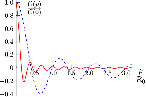
Refer to caption
Figure 6.2: Correlation function of the component ΣzzsubscriptΣ𝑧𝑧\Sigma_{zz} of the stress tensor normalized by it’s value at ρ=0𝜌0\rho=0 as a function of ρ/R0𝜌subscript𝑅0\rho/R_{0}. In both curves, we considered tubes of length 500nm500nm500\,\mathrm{nm} and bending rigidity κ=50kBT𝜅50subscript𝑘B𝑇\kappa=50\,k_{\mathrm{B}}T. We have chosen Λ1=5nmsuperscriptΛ15nm\Lambda^{-1}=5\,\mathrm{nm} as the value of the microscopical cut-off. The blue dashed curve stands for a thin tube with R0=30nmsubscript𝑅030nmR_{0}=30\,\mathrm{nm}, while the red solid curve stands for a tube with R0=100nmsubscript𝑅0100nmR_{0}=100\,\mathrm{nm}.

First of all, we note that even though the stress tensor correlation decreases with the distance, we have no more the fast decay found in the case of planar membranes (see section 3.4). In both cases, the function C(ρ)𝐶𝜌C(\rho) presents oscillations that remain non negligible throughout the whole section of the tube, indicating that the stress tensor is correlated all over the length of a tube’s cross section. This is a signature of the fact that the fluctuations in the shape of membrane tubes are themselves correlated over a whole cross section, whatever the tube’s radius [7]. Moreover, we observe that the oscillations in Fig. 6.2 take place over a roughly constant wave-length λ𝜆\lambda. For the tube with R0=30nmsubscript𝑅030nmR_{0}=30\,\mathrm{nm}, we have 666 oscillations distributed over the perimeter, which gives a wave-length λ31nm6Λ1𝜆31nmsimilar-to6superscriptΛ1\lambda\approx 31\,\mathrm{nm}\sim 6\,\Lambda^{-1}, with Λ15nmsimilar-tosuperscriptΛ15nm\Lambda^{-1}\sim 5\,\mathrm{nm}. Interestingly, we find the same value for the larger tube. This characteristic wave-length corresponds to the length beyond which the correlation of the stress tensor in planar membranes becomes negligible (see section 3.4). It is thus probably an universal quantity, valid for any value of R0subscript𝑅0R_{0}.

To characterize better how the stress tensor correlation decreases, we have plotted the absolute value of the extrema of the oscillations of the red curve as a function of ρ/R0𝜌subscript𝑅0\rho/R_{0} in a log-log scale (see Fig. 6.3). This curve seems to indicate that the amplitude of the oscillations decay with a power law, which is a characteristic sign of long-range correlations.
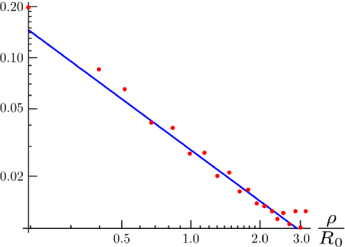
Refer to caption
Figure 6.3: The red dots represent the absolute value of the extrema of the red solid curve in Fig. 6.2 as a function of ρ/R0𝜌subscript𝑅0\rho/R_{0}. The blue solid curve is proportional to x1superscript𝑥1x^{-1}.

Finally, we have compared the contribution of the first term of eq.(6.110), involving two sums over the wavenumbers, and the contribution of the second term of eq.(6.110), with an unique sum over the wavenumbers, to the total stress tensor correlation. As one can see in Fig. 6.4(a) and in Fig. 6.4(b), in general, both contributions are oscillating and important. In the following, however, we will see that the second term of eq.(6.110), with an unique sum and represented by the solid lines in these figures, gives a vanishing contribution to ΔfzΔsubscript𝑓𝑧\Delta f_{z}.

Refer to caption
(a) Tube with R0=30nmsubscript𝑅030nmR_{0}=30\,\mathrm{nm}.
Refer to caption
(b) Tube with R0=100nmsubscript𝑅0100nmR_{0}=100\,\mathrm{nm}.
Figure 6.4: Contribution of the first term of eq.(6.110) (term with the double sum over the wavenumbers) to the stress tensor correlation (red dashed line) compared to the contribution of the second term of this equation, with an unique sum over the wavenumbers (blue solid curve). In both cases, we have considered tubes with length 500nm500nm500\,\mathrm{nm}, κ=50kBT𝜅50subscript𝑘B𝑇\kappa=50\,k_{\mathrm{B}}T and Λ1=5nmsuperscriptΛ15nm\Lambda^{-1}=5\,\mathrm{nm}.
6.3.2 Force fluctuation 𝚫𝒇𝒛𝚫subscript𝒇𝒛\bm{\Delta f_{z}}

As we have seen in eq.(6.7), the force fluctuation is given by

(Δfz)2superscriptΔsubscript𝑓𝑧2\displaystyle(\Delta f_{z})^{2} =\displaystyle= 02πR002πR0C(ρ,ρ)𝑑ρ𝑑ρ,superscriptsubscript02𝜋subscript𝑅0superscriptsubscript02𝜋subscript𝑅0𝐶𝜌superscript𝜌differential-d𝜌differential-dsuperscript𝜌\displaystyle\int_{0}^{2\pi R_{0}}\int_{0}^{2\pi R_{0}}C(\rho,\rho^{\prime})\,d\rho d\rho^{\prime}\,, (6.113)
=\displaystyle= 02πR002πR0C(ρρ,0)𝑑ρ𝑑ρ.superscriptsubscript02𝜋subscript𝑅0superscriptsubscript02𝜋subscript𝑅0𝐶𝜌superscript𝜌0differential-d𝜌differential-dsuperscript𝜌\displaystyle\int_{0}^{2\pi R_{0}}\int_{0}^{2\pi R_{0}}C(\rho-\rho^{\prime},0)\,d\rho d\rho^{\prime}\,.

The last passage follows from the fact that the correlation function is invariant under translation. The function C(ρ,0)𝐶𝜌0C(\rho,0) is periodic with period 2πR02𝜋subscript𝑅02\pi R_{0}. Consequently, eq.(6.113) is equivalent to

(Δfz)2=2πR002πR0C(ρ′′,0)𝑑ρ′′.superscriptΔsubscript𝑓𝑧22𝜋subscript𝑅0superscriptsubscript02𝜋subscript𝑅0𝐶superscript𝜌′′0differential-dsuperscript𝜌′′(\Delta f_{z})^{2}=2\pi R_{0}\int_{0}^{2\pi R_{0}}C(\rho^{\prime\prime},0)\,d\rho^{\prime\prime}\,. (6.114)

Using the fact that

02πR0eiR01(m+n)ρ′′𝑑ρ′′=2πR0δn,m,superscriptsubscript02𝜋subscript𝑅0superscript𝑒𝑖superscriptsubscript𝑅01𝑚𝑛superscript𝜌′′differential-dsuperscript𝜌′′2𝜋subscript𝑅0subscript𝛿𝑛𝑚\int_{0}^{2\pi R_{0}}e^{iR_{0}^{-1}(m+n)\rho^{\prime\prime}}\,d\rho^{\prime\prime}=2\pi R_{0}\,\delta_{n,-m}\,, (6.115)

we obtain

(Δfz)2superscriptΔsubscript𝑓𝑧2\displaystyle(\Delta f_{z})^{2} =\displaystyle= (2πR0)2(kBT4πR0L)2m,q¯k¯fm,m,q¯,k¯,superscript2𝜋subscript𝑅02superscriptsubscript𝑘𝐵𝑇4𝜋subscript𝑅0𝐿2subscript𝑚¯𝑞subscript¯𝑘subscript𝑓𝑚𝑚¯𝑞¯𝑘\displaystyle(2\pi R_{0})^{2}\left(\frac{k_{B}T}{4\pi R_{0}L}\right)^{2}\sum_{m,\bar{q}}\sum_{\bar{k}}f_{-m,m,\bar{q},\bar{k}}\,,
=\displaystyle= (kBT2L)2m,q¯k¯2(m21)4+4k¯2q¯2[k¯41+2m2(1+2k¯2)+m4]+6k¯4q¯4[(m21)2+q¯2(q¯2+2m2)][(m21)2+k¯2(k¯2+2m2)].superscriptsubscript𝑘B𝑇2𝐿2subscript𝑚¯𝑞subscript¯𝑘2superscriptsuperscript𝑚2144superscript¯𝑘2superscript¯𝑞2delimited-[]superscript¯𝑘412superscript𝑚212superscript¯𝑘2superscript𝑚46superscript¯𝑘4superscript¯𝑞4delimited-[]superscriptsuperscript𝑚212superscript¯𝑞2superscript¯𝑞22superscript𝑚2delimited-[]superscriptsuperscript𝑚212superscript¯𝑘2superscript¯𝑘22superscript𝑚2\displaystyle\left(\frac{k_{\mathrm{B}}T}{2L}\right)^{2}\sum_{m,\bar{q}}\sum_{\bar{k}}\frac{2(m^{2}-1)^{4}+4\bar{k}^{2}\bar{q}^{2}\left[\bar{k}^{4}-1+2m^{2}\left(1+2\bar{k}^{2}\right)+m^{4}\right]+6\bar{k}^{4}\bar{q}^{4}}{\left[(m^{2}-1)^{2}+\bar{q}^{2}(\bar{q}^{2}+2m^{2})\right]\,\left[(m^{2}-1)^{2}+\bar{k}^{2}(\bar{k}^{2}+2m^{2})\right]}\,.

Note that the contribution of the last term of eq.(6.110) vanishes after integration.

Long tubes

For the case of L>R0𝐿subscript𝑅0L>R_{0}, we can substitute the sums over q¯¯𝑞\bar{q} and over k¯¯𝑘\bar{k} by integrals, yielding

(Δfz)2=(kBT4πR0)2m=MMΛR0ΛR0ΛR0ΛR02(m21)4+4k¯2q¯2[k¯41+2m2(1+2k¯2)+m4]+6k¯4q¯4[(m21)2+q¯2(q¯2+2m2)][(m21)2+k¯2(k¯2+2m2)]𝑑q¯𝑑k¯.superscriptΔsubscript𝑓𝑧2superscriptsubscript𝑘B𝑇4𝜋subscript𝑅02superscriptsubscript𝑚𝑀𝑀superscriptsubscriptΛsubscript𝑅0Λsubscript𝑅0superscriptsubscriptΛsubscript𝑅0Λsubscript𝑅02superscriptsuperscript𝑚2144superscript¯𝑘2superscript¯𝑞2delimited-[]superscript¯𝑘412superscript𝑚212superscript¯𝑘2superscript𝑚46superscript¯𝑘4superscript¯𝑞4delimited-[]superscriptsuperscript𝑚212superscript¯𝑞2superscript¯𝑞22superscript𝑚2delimited-[]superscriptsuperscript𝑚212superscript¯𝑘2superscript¯𝑘22superscript𝑚2differential-d¯𝑞differential-d¯𝑘\begin{split}&(\Delta f_{z})^{2}=\\ &\left(\frac{k_{\mathrm{B}}T}{4\pi R_{0}}\right)^{2}\!\sum_{m=-M}^{M}\int_{-\Lambda R_{0}}^{\Lambda R_{0}}\int_{-\Lambda R_{0}}^{\Lambda R_{0}}\frac{2(m^{2}-1)^{4}+4\bar{k}^{2}\bar{q}^{2}\left[\bar{k}^{4}-1+2m^{2}\left(1+2\bar{k}^{2}\right)+m^{4}\right]+6\bar{k}^{4}\bar{q}^{4}}{\left[(m^{2}-1)^{2}+\bar{q}^{2}(\bar{q}^{2}+2m^{2})\right]\,\left[(m^{2}-1)^{2}+\bar{k}^{2}(\bar{k}^{2}+2m^{2})\right]}\,d\bar{q}\,d\bar{k}\,.\end{split} (6.117)

Taking into account the fact that eq.(6.117) depends only on |m|𝑚|m|, it can be rewritten as

(Δfz)2=(kBT4πR0)2(T0+2T1+2m=2MTm),superscriptΔsubscript𝑓𝑧2superscriptsubscript𝑘B𝑇4𝜋subscript𝑅02subscript𝑇02subscript𝑇12superscriptsubscript𝑚2𝑀subscript𝑇𝑚(\Delta f_{z})^{2}=\left(\frac{k_{\mathrm{B}}T}{4\pi R_{0}}\right)^{2}\!\left(T_{0}+2\,T_{1}+2\,\sum_{m=2}^{M}T_{m}\right)\,, (6.118)

with

T0=ΛR0ΛR0ΛR0ΛR02q¯4k¯4(q¯2+k¯2)+(1q¯2k¯2)2(1+q¯4)(1+k¯4)𝑑q¯𝑑k¯,subscript𝑇0superscriptsubscriptΛsubscript𝑅0Λsubscript𝑅0superscriptsubscriptΛsubscript𝑅0Λsubscript𝑅02superscript¯𝑞4superscript¯𝑘4superscript¯𝑞2superscript¯𝑘2superscript1superscript¯𝑞2superscript¯𝑘221superscript¯𝑞41superscript¯𝑘4differential-d¯𝑞differential-d¯𝑘T_{0}=\int_{-\Lambda R_{0}}^{\Lambda R_{0}}\int_{-\Lambda R_{0}}^{\Lambda R_{0}}\frac{2\bar{q}^{4}\bar{k}^{4}\left(\bar{q}^{2}+\bar{k}^{2}\right)+\left(1-\bar{q}^{2}\bar{k}^{2}\right)^{2}}{\left(1+\bar{q}^{4}\right)\left(1+\bar{k}^{4}\right)}\,d\bar{q}\,d\bar{k}\,, (6.119)
T1=ΛR0ΛR0ΛR0ΛR08+4k¯4+2k¯2(8+3q¯2)(2+q¯2)(2+k¯2)𝑑q¯𝑑k¯,subscript𝑇1superscriptsubscriptΛsubscript𝑅0Λsubscript𝑅0superscriptsubscriptΛsubscript𝑅0Λsubscript𝑅084superscript¯𝑘42superscript¯𝑘283superscript¯𝑞22superscript¯𝑞22superscript¯𝑘2differential-d¯𝑞differential-d¯𝑘T_{1}=\int_{-\Lambda R_{0}}^{\Lambda R_{0}}\int_{-\Lambda R_{0}}^{\Lambda R_{0}}\frac{8+4\bar{k}^{4}+2\bar{k}^{2}\left(8+3\bar{q}^{2}\right)}{\left(2+\bar{q}^{2}\right)\left(2+\bar{k}^{2}\right)}\,d\bar{q}\,d\bar{k}\,, (6.120)

and

Tm=ΛR0ΛR0ΛR0ΛR02(m21)4+4k¯2q¯2[k¯41+2m2(1+2k¯2)+m4]+6k¯4q¯4[(m21)2+q¯2(q¯2+2m2)][(m21)2+k¯2(k¯2+2m2)]𝑑q¯𝑑k¯.subscript𝑇𝑚superscriptsubscriptΛsubscript𝑅0Λsubscript𝑅0superscriptsubscriptΛsubscript𝑅0Λsubscript𝑅02superscriptsuperscript𝑚2144superscript¯𝑘2superscript¯𝑞2delimited-[]superscript¯𝑘412superscript𝑚212superscript¯𝑘2superscript𝑚46superscript¯𝑘4superscript¯𝑞4delimited-[]superscriptsuperscript𝑚212superscript¯𝑞2superscript¯𝑞22superscript𝑚2delimited-[]superscriptsuperscript𝑚212superscript¯𝑘2superscript¯𝑘22superscript𝑚2differential-d¯𝑞differential-d¯𝑘T_{m}=\int_{-\Lambda R_{0}}^{\Lambda R_{0}}\int_{-\Lambda R_{0}}^{\Lambda R_{0}}\frac{2(m^{2}-1)^{4}+4\bar{k}^{2}\bar{q}^{2}\left[\bar{k}^{4}-1+2m^{2}\left(1+2\bar{k}^{2}\right)+m^{4}\right]+6\bar{k}^{4}\bar{q}^{4}}{\left[(m^{2}-1)^{2}+\bar{q}^{2}(\bar{q}^{2}+2m^{2})\right]\,\left[(m^{2}-1)^{2}+\bar{k}^{2}(\bar{k}^{2}+2m^{2})\right]}\,d\bar{q}\,d\bar{k}\,. (6.121)

Both integrals over q¯¯𝑞\bar{q} and over k¯¯𝑘\bar{k} in eq.(6.119), eq.(6.120) and eq.(6.121) can be performed analytically. One can compare the contributions of some modes to the force fluctuation in Fig. 6.5. Not surprisingly, the modes |m|=1𝑚1|m|=1, which are extremely soft [7], give a greater contribution.
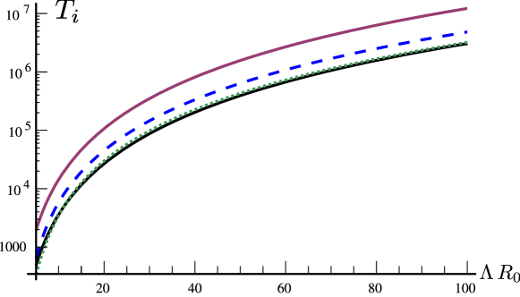
Refer to caption
Figure 6.5: For very long tubes, each radial mode i𝑖i gives a contribution [kBT/(4πR0)]2×Tisuperscriptdelimited-[]subscript𝑘B𝑇4𝜋subscript𝑅02subscript𝑇𝑖[k_{\mathrm{B}}T/(4\pi R_{0})]^{2}\times T_{i} to (Δfz)2superscriptΔsubscript𝑓𝑧2(\Delta f_{z})^{2}, with Tisubscript𝑇𝑖T_{i} given by eqs.(6.119)–(6.121). We compare here the contributions of the modes with m=0𝑚0m=0 (lower solid line, in black), m=1𝑚1m=1 (upper solid line, in red), m=2𝑚2m=2 (dashed blue line) and m=3𝑚3m=3 (dotted green line) as a function of the tube’s radius. The vertical scale is shown in units of [kBT/(4πR0)]2superscriptdelimited-[]subscript𝑘B𝑇4𝜋subscript𝑅02[k_{\mathrm{B}}T/(4\pi R_{0})]^{2}, while the radius of the tube is shown in units of the microscopical cutoff a=Λ1𝑎superscriptΛ1a=\Lambda^{-1}. We see that the Goldstone modes, with m=1𝑚1m=1, give indeed a greater contribution to the force fluctuation.

In Fig. 6.6, we show the percent contribution of these soft modes to the total fluctuation. In agreement with the curves of Fig. 6.5, the modes with |m|=1𝑚1|m|=1 are responsible for more than one third of the force fluctuation.
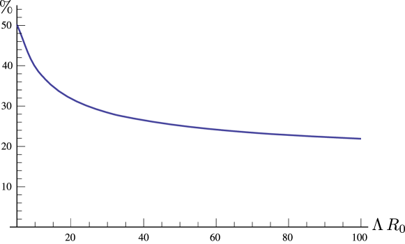
Refer to caption
Figure 6.6: Percent contribution of the soft modes (|m|=1𝑚1|m|=1) to the total force fluctuation.
Approximations and an analytical formula for 𝚫𝒇𝒛𝚫subscript𝒇𝒛\bm{\Delta f_{z}}

In order to obtain a simple analytical expression to the force fluctuation, we consider the limit of relatively thick tubes, with ΛR0>6Λsubscript𝑅06\Lambda\,R_{0}>6. Considering a=Λ1=5nm𝑎superscriptΛ15nma=\Lambda^{-1}=5\,\mathrm{nm}, this corresponds to tubes with a radius R0>30nmsubscript𝑅030nmR_{0}>30\,\mathrm{nm}, which is currently observed in experiments. In this limit, we have

T022π3(ΛR0)3,subscript𝑇022𝜋3superscriptΛsubscript𝑅03T_{0}\approx\frac{2\sqrt{2}\pi}{3}\,(\Lambda\,R_{0})^{3}\,, (6.122)
T142π3(ΛR0)3,subscript𝑇142𝜋3superscriptΛsubscript𝑅03T_{1}\approx\frac{4\sqrt{2}\pi}{3}\,(\Lambda\,R_{0})^{3}\,, (6.123)

and

Tm24(ΛR0)2+83m[(ΛR0)321m2(ΛR0)+12m3arctan(ΛR0m)]arctan(ΛR0m).subscript𝑇𝑚24superscriptΛsubscript𝑅0283𝑚delimited-[]superscriptΛsubscript𝑅0321superscript𝑚2Λsubscript𝑅012superscript𝑚3Λsubscript𝑅0𝑚Λsubscript𝑅0𝑚\displaystyle T_{m}\approx 24(\Lambda\,R_{0})^{2}+\frac{8}{3m}\left[(\Lambda\,R_{0})^{3}-21m^{2}(\Lambda\,R_{0})+12m^{3}\arctan\left(\frac{\Lambda\,R_{0}}{m}\right)\right]\arctan\left(\frac{\Lambda\,R_{0}}{m}\right)\,.

The sum over m𝑚m in eq.(6.118) can be approximated by an integral, yielding

m=2MTm2ΛR0Tm𝑑m22π3(ΛR0)3+4π3(ΛR0)3ln(ΛR0).superscriptsubscript𝑚2𝑀subscript𝑇𝑚superscriptsubscript2Λsubscript𝑅0subscript𝑇𝑚differential-d𝑚similar-to-or-equals22𝜋3superscriptΛsubscript𝑅034𝜋3superscriptΛsubscript𝑅03Λsubscript𝑅0\sum_{m=2}^{M}T_{m}\approx\int_{2}^{\Lambda\,R_{0}}T_{m}\,dm\simeq\frac{2\sqrt{2}\pi}{3}\,(\Lambda\,R_{0})^{3}\,+\frac{4\pi}{3}\,(\Lambda\,R_{0})^{3}\,\ln(\Lambda\,R_{0})\,. (6.125)

At last, we obtain

(Δfz)2(kBT)2R0Λ36π[52+ln(ΛR0)].similar-to-or-equalssuperscriptΔsubscript𝑓𝑧2superscriptsubscript𝑘B𝑇2subscript𝑅0superscriptΛ36𝜋delimited-[]52Λsubscript𝑅0\left(\Delta f_{z}\right)^{2}\simeq\frac{(k_{\mathrm{B}}T)^{2}\,R_{0}\,\Lambda^{3}}{6\pi}\left[\frac{5}{2}+\ln\left(\Lambda\,R_{0}\right)\right]\,. (6.126)

We discuss the quality of this approximation and its meaning in section 6.4.

6.3.3 Discussion on the validity of this result

Here we remind the conditions of validity of eq.(6.118). First, denoting u𝑢u the deformation of the tube relative to the mean-field cylinder, we considered here only terms up to 𝒪(u2)𝒪superscript𝑢2\mathcal{O}(u^{2}) in the Hamiltonian and in the stress tensor. Accordingly, our result corresponds actually to the first term in a series expansion of the form

(Δfz)2=f02[(kBTκ)2g1(ΛR0)+(kBTκ)3g2(ΛR0)+].superscriptΔsubscript𝑓𝑧2superscriptsubscript𝑓02delimited-[]superscriptsubscript𝑘B𝑇𝜅2subscript𝑔1Λsubscript𝑅0superscriptsubscript𝑘B𝑇𝜅3subscript𝑔2Λsubscript𝑅0(\Delta f_{z})^{2}=f_{0}^{2}\left[\left(\frac{k_{\mathrm{B}}T}{\kappa}\right)^{2}\,g_{1}(\Lambda\,R_{0})+\left(\frac{k_{\mathrm{B}}T}{\kappa}\right)^{3}\,g_{2}(\Lambda\,R_{0})+\cdots\right]\,. (6.127)

The term (kBT)2proportional-toabsentsuperscriptsubscript𝑘B𝑇2\propto(k_{\mathrm{B}}T)^{2} corresponds to the contributions of terms up to order two in u𝑢u, coming from the diagrams of the form [Uncaptioned image] . Further terms of higher order on kBTsubscript𝑘B𝑇k_{\mathrm{B}}T come from the terms beyond 𝒪(u2)𝒪superscript𝑢2\mathcal{O}(u^{2}) in the Hamiltonian and in the stress tensor. Secondly, eq.(6.118) is valid for tubes relatively long, i. e., whose length is bigger than the radius, but still small compared to the radius of the vesicle from which it is extracted. The simplified eq.(6.126) is a good approximation under the supplemental condition ΛR0>6Λsubscript𝑅06\Lambda\,R_{0}>6.

Finally, let us comment on the influence of the boundary conditions. Differently from the case of the average force, there is no conservation principle for ΔfzΔsubscript𝑓𝑧\Delta f_{z}. Here, we have calculated ΔfzΔsubscript𝑓𝑧\Delta f_{z} assuming periodic boundary conditions, or equivalently, through an arbitrary section in the middle of a long enough tube. The actual value of ΔfzΔsubscript𝑓𝑧\Delta f_{z} at the extremity of a tubule with specific boundary conditions might be somewhat different. Note also that we have only calculated the fluctuation of the component of the force which is parallel to the tube axis.

6.4 Discussion and consequences for experiments

First of all, let us discuss on the dependence of ΔfzΔsubscript𝑓𝑧\Delta f_{z} on R0subscript𝑅0R_{0}. From eq.(6.126), we have

ΔfzR0a(kBTa)×ln(R0a),proportional-toΔsubscript𝑓𝑧subscript𝑅0𝑎subscript𝑘B𝑇𝑎subscript𝑅0𝑎\Delta f_{z}\propto\sqrt{\frac{R_{0}}{a}}\left(\frac{k_{\mathrm{B}}T}{a}\right)\times\sqrt{\ln\left(\frac{R_{0}}{a}\right)}\,, (6.128)

with a=Λ1𝑎superscriptΛ1a=\Lambda^{-1} of the order of the membrane thickness. The first term reminds the result obtained in chapter 3. There, we have seen that for planar membranes, the correlation of the stress tensor decreases over a very short length, whatever the membrane tension or rigidity. One could thus consider that a piece of membrane was a composition of uncorrelated patches of size aabsent𝑎\approx a and use the Central Limit Theorem to obtain the force fluctuation. In this case, however, the force fluctuation of tubes has a supplemental logarithmic correction relative to force fluctuation in planar membranes. This correction can be explained by the fact that the correlation of the stress tensor in membrane nanotubes decreases in a power law, as we have shown in section 6.3.1.

In Fig. 6.7, we show ΔfzΔsubscript𝑓𝑧\Delta f_{z} as a function on R0subscript𝑅0R_{0} for different values of the cutoff ΛΛ\Lambda. The exact curve for long tubes given in eq.(6.118) is indicated by circles, while the approximation given in eq.(6.126) corresponds to the solid lines. We can see the good quality of the approximation. For a given value of ΛΛ\Lambda, ΔfzΔsubscript𝑓𝑧\Delta f_{z} does not vary much over the experimental range of R0subscript𝑅0R_{0}. On the contrary, it depends strongly on the value of the cutoff ΛΛ\Lambda.

Numerically, we have found a force fluctuation of some pNpN\mathrm{pN}, which is of the same order of magnitude of the value obtained experimentally experimentally (see Fig. 6.1, [98] and [119]). For an accurate comparison, however, time-resolved measurements should be performed and the Brownian force on the pulling bead should be taken into account.
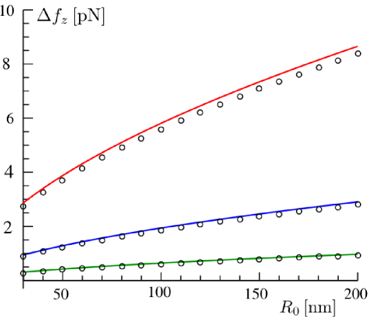
Refer to caption
Figure 6.7: Force fluctuation as a function of the tube’s radius. The solid lines correspond to the approximation given in eq.(6.126). The curves for Λa=2, 1,0.5Λ𝑎210.5\Lambda\,a=2,\,1\,,0.5 are shown, respectively, in blue (curve in the middle), red (upper curve) and green (lower curve). The circles stand for the exact numerical sum (eq.(6.118)). Remark the good quality of the approximation. In this plot, we have considered kBT=4×10²¹Jsubscript𝑘B𝑇4superscript1021Jk_{\mathrm{B}}T=4\times 10^{-21}\,\mathrm{J} and a=5nm𝑎5nma=5\,\mathrm{nm}.

Finally, we compare the average of the force needed to extract a tube, given by eq.(5.72), with it’s fluctuation. We trace both curves as a function of the effective mechanical tension τ𝜏\tau, since this tension can be experimentally controlled (by changing the difference of pressure in micropipettes experiments, for instance). In agreement with the results of the previous chapters, we assume τ=σσ0𝜏𝜎subscript𝜎0\tau=\sigma-\sigma_{0}, where σ0=(kBTΛ2)/(8π)subscript𝜎0subscript𝑘B𝑇superscriptΛ28𝜋\sigma_{0}=(k_{\mathrm{B}}T\,\Lambda^{2})/(8\pi). Applying this relation to eq.(6.126), we obtain

(Δfz)2(kBT)2Λ36πκ2(τ+σ0)[52+ln(Λκ2(τ+σ0))].similar-to-or-equalssuperscriptΔsubscript𝑓𝑧2superscriptsubscript𝑘B𝑇2superscriptΛ36𝜋𝜅2𝜏subscript𝜎0delimited-[]52Λ𝜅2𝜏subscript𝜎0\left(\Delta f_{z}\right)^{2}\simeq\frac{(k_{\mathrm{B}}T)^{2}\,\Lambda^{3}}{6\pi}\sqrt{\frac{\kappa}{2(\tau+\sigma_{0})}}\left[\frac{5}{2}+\ln\left(\Lambda\,\sqrt{\frac{\kappa}{2(\tau+\sigma_{0})}}\right)\right]\,. (6.129)

The curve for fzdelimited-⟨⟩subscript𝑓𝑧\langle f_{z}\rangle, already presented in Fig. 5.10 and the curve of ΔfzΔsubscript𝑓𝑧\Delta f_{z} given above is shown in Fig. 6.8. We can remark that ΔfzΔsubscript𝑓𝑧\Delta f_{z} is in general small compared to the force fzsubscript𝑓𝑧f_{z} needed to extract a tube, despite the presence of soft Goldstone modes: it is comparable to fzsubscript𝑓𝑧f_{z} for τ<106J/m2𝜏superscript106Jsuperscriptm2\tau<10^{-6}\mathrm{J/m}^{2}, but quite negligible for τ>105J/m2𝜏superscript105Jsuperscriptm2\tau>10^{-5}\mathrm{J/m}^{2}.

Refer to caption

Figure 6.8: Average force needed to pull a tube (solid red line) and it’s fluctuation ΔfzΔsubscript𝑓𝑧\Delta f_{z} (dashed blue line) as a function of the effective mechanical tension τ𝜏\tau. The parameters used are Λa=1Λ𝑎1\Lambda\,a=1 with a5nmsimilar-to-or-equals𝑎5nma\simeq 5\,\mathrm{nm}, kBT4×1021Jsimilar-to-or-equalssubscript𝑘𝐵𝑇4superscript1021Jk_{B}T\simeq 4\times 10^{-21}\,\mathrm{J} and κ50kBTsimilar-to-or-equals𝜅50subscript𝑘𝐵𝑇\kappa\simeq 50\,k_{B}T.

Sadly, from Fig. 6.7 and 6.8, we conclude that ΔfzΔsubscript𝑓𝑧\Delta f_{z} does almost not depend on the tension of the membrane nor on it’s rigidity. The force fluctuation seems thus of little interest in the mechanical characterization of membranes. On the other hand, the fact that ΔfzΔsubscript𝑓𝑧\Delta f_{z} does not depend neither in κ𝜅\kappa, neither on the membrane tension, could be of great interest to experiments involving active membranes. Differently from the membranes studied in this work, which are passive, active membranes have proteins embedded in it that add non-equilibrium noise to the system. Experimentally, the activity of these proteins depends on a external source of energy. It has been observed that the protein activity causes an enhancement of the membrane fluctuations and of the excess area relative to the passive case, as if the membrane were in contact with a thermal bath of higher temperature [121]. Let’s imagine now an experiment in which tubes were extracted from an active membrane. If the membrane fluctuations were intensified, ΔfzΔsubscript𝑓𝑧\Delta f_{z} should be also affected. Since it does almost not depend on the tension nor on the bending rigidity, it could thus be a used as a direct indicator of the proteins activity.

6.5 In a nutshell

In this chapter, we have examined the possibility of using the fluctuation of the force along a membrane tube’s axis ΔfzΔsubscript𝑓𝑧\Delta f_{z} as a tool to characterize membranes. We have only considered the contribution of the membrane’s fluctuation, that can be very important due to the presence of very soft modes. For a weakly fluctuating tube of length L𝐿L, with RvesL>R0much-greater-thansubscript𝑅ves𝐿subscript𝑅0R_{\mathrm{ves}}\gg L>R_{0}, where Rvessubscript𝑅vesR_{\mathrm{ves}} is the radius of the vesicle from which the tube is pulled and R0subscript𝑅0R_{0} is the mean-field radius of the tube, we obtained

(Δfz)2(kBT)2R0Λ36π[52+ln(ΛR0)],similar-to-or-equalssuperscriptΔsubscript𝑓𝑧2superscriptsubscript𝑘B𝑇2subscript𝑅0superscriptΛ36𝜋delimited-[]52Λsubscript𝑅0\left(\Delta f_{z}\right)^{2}\simeq\frac{(k_{\mathrm{B}}T)^{2}\,R_{0}\,\Lambda^{3}}{6\pi}\left[\frac{5}{2}+\ln\left(\Lambda\,R_{0}\right)\right]\,, (6.130)

where Λ1=asuperscriptΛ1𝑎\Lambda^{-1}=a, with a𝑎a of the order of the membrane thickness. Interestingly, ΔfzΔsubscript𝑓𝑧\Delta f_{z} can generally be written as

ΔfzR0a(kBTa)×ln(R0a),proportional-toΔsubscript𝑓𝑧subscript𝑅0𝑎subscript𝑘B𝑇𝑎subscript𝑅0𝑎\Delta f_{z}\propto\sqrt{\frac{R_{0}}{a}}\left(\frac{k_{\mathrm{B}}T}{a}\right)\times\sqrt{\ln\left(\frac{R_{0}}{a}\right)}\,, (6.131)

which reminds the result found for the force fluctuation in planar membranes. The logarithmic correction is a signature of the long-range correlations present in the tubes. Numerically, for a5nm𝑎5nma\approx 5\,\mathrm{nm}, these equations yield Δfz1pNΔsubscript𝑓𝑧1pN\Delta f_{z}\approx 1\mathrm{pN}, which is compatible with experimental data. Studying the behavior of the force fluctuation, we have found that it is extremely sensitive to the value of ΛΛ\Lambda, whereas it does almost not depend on the bending rigidity nor on the tension. Thus, ΔfzΔsubscript𝑓𝑧\Delta f_{z} seems of little usefulness to the mechanical characterization of membranes. It could however be used in experiments involving active membranes, i. e., membranes containing proteins whose activity can be modified, as an indicator of their activity. Indeed, when proteins are active, the membrane fluctuations are increased, which would affect ΔfzΔsubscript𝑓𝑧\Delta f_{z} regardless of variations on the bending rigidity or on the tension.

Part IV Preliminar works on a 2-D simulation

Chapter 7 Preliminary results on a 𝟐2\bm{2}-d membrane simulation

In section 2.3, we proposed a simple numerical system to verify our predictions concerning the mechanical tension τ𝜏\tau, the internal tension σ𝜎\sigma and the tension r𝑟r obtained from the fluctuation spectrum of a membrane. Our model was composed of a set of variable-sized rods, each one representing a coarse-graining of several lipids, free to move in a two-dimensional space.

In this chapter, we present a more complex numerical experiment consisting of a 222-dimensional membrane that evolves in a three-dimensional space, which corresponds more accurately to the experimental situation. We are motivated by the fact that a more elaborated numerical system would not only allow us to verify precisely our predictions concerning τ𝜏\tau, σ𝜎\sigma and r𝑟r, but it would also give access to other quantities, such as the fluctuation of the force that a frame exerts over a membrane, studied in chapter 3. Moreover, in chapters 5 and 6 we predict the dependence of the force needed to extract a tube and its fluctuation on τ𝜏\tau, which could also be verified by pulling tubes from a numerical membrane. Sadly, due to time constraints, the results presented here are far from complete and many questions are left unanswered.

In our numerical experiment, we would like to study a piece of membrane held by a circular frame and weakly departing from a plane (see Fig. 7.1). We find many popular methods used to numerically simulate membranes in the scientific literature, which we sum-up briefly in section 7.1. We have chosen to use a phenomenological model consisting in a triangular network of extensible bonds connecting effective particles. The connectivity of the network could be modified in order to mimic the membrane’s liquidity (see details in section 7.2) and a harmonic potential acted over the particles at the network’s edge, forcing a circular frame. Thus, we could measure directly the force applied to the frame and derive the effective tension τ𝜏\tau as well as its fluctuation ΔτΔ𝜏\Delta\tau (see section 7.4.1). The minima of this potential could be modified to widen the frame’s radius, decreasing the excess area α𝛼\alpha and increasing the membrane’s tension.
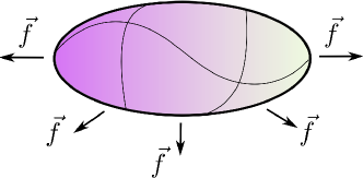
Refer to caption
Figure 7.1: Numerical experiment: a fluctuating membrane weakly departing from a plane held by a circular frame. A force could be applied to the frame in order to widen its radius, increasing thus the membrane’s effective tension.

To obtain representative averages of τ𝜏\tau, α𝛼\alpha and other variables, we needed to generate large sets of configurations of the numerical membrane, which was done through a Monte Carlo dynamics, described in section 7.3. In this section, we discuss also which were the criteria used by us to determine whether a sampling was large enough.

As usually done in laboratory experiments (see section 1.4.2), the bending rigidity κ𝜅\kappa and tension r𝑟r were deduced from the average of the fluctuation spectrum of the membrane. Since we simulate the membrane using a network, obtaining the fluctuation spectrum is somewhat complicated, as we discuss in section 7.4.2. Finally, we explain in section 7.4.3 how we could estimate the internal tension σ𝜎\sigma. In section 7.5 we discuss some preliminary results. At last, in section 7.6, we comment briefly on extracting tubes from our numerical membrane and we end this chapter with a brief discussion on issues that should be investigated in the future (section 7.7).

7.1 Short panorama of numerical models on membranes

Processes in membranes happen in a wide range of time, size and energy scales. For instance, interactions between lipids and proteins inside the membrane occur in distances of the order of the nanometer with a characteristic time of some psps\mathrm{ps}, while the evolution of the shape of a vesicle involves scales of micrometers and may take many seconds. Consequently, depending on the process one is interested in, several different models are used to numerically simulate biological membranes (see [122], [123] and [124] for some reviews). Schematically, they can be grouped in three classes:
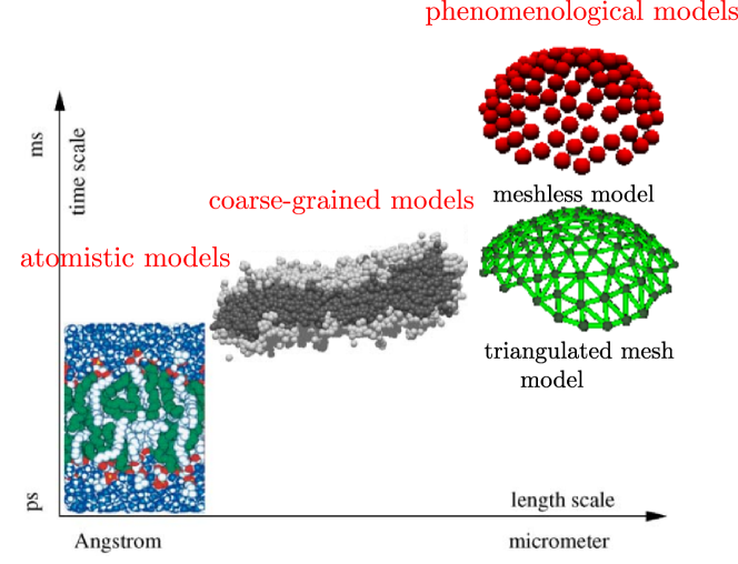
Refer to caption
Figure 7.2: Illustration of the three main classes of numerical models used to simulate biological membranes, ordered in terms of the characteristic time and length scale (figure based on [122]).
  1. 1.

    atomistic models: these models try to take into account all the chemical details of the molecules by considering the interactions between atoms. They are used to study how lipids interact among themselves and with proteins. As these simulations involve many degrees of freedom, they are very computer consuming. Consequently, one can at most simulate small patches of a dozen of nanometers for dozens of nanoseconds.

  2. 2.

    coarse-grained models: in these models, small groups of atoms are lumped together into effective particles that interact via simplified potentials. The solvent can be effectively or implicitly present. As the number of degrees of freedom is reduced, one can observe collective movements of the membrane, such as its self-assembly, stretching [109], pore formation [109] and thermal fluctuations [3]. The main difficulty of these models is deciding which interactions are truly essential to reproduce the membrane’s behavior. A popular model of this category is the spring-and-bead model presented in section 2.5. Sadly, with these models one is still restrained to length scales of hundreds of nanometers, which is a limitation if one wants to study large-scale processes.

  3. 3.

    phenomenological models: these models take coarse-graining one step further, representing several molecules as a single effective particle, which we will call a bead in the following. The solvent is always implicit. They are suitable to study the universal properties of amphiphilic systems. The effective particles can be attached between themselves through a triangular or square mesh or instead, the mesh can be absent [125],  [126] (meshless models). In the first case, to mimic liquidity, the topology of the mesh is changed during the simulation. The meshwork is then called dynamic. Our previous simple model, presented in section 2.3, belong to this category.

Throughout this work, we were interested in the general properties of membranes, regardless of the molecular details, at length scales far bigger than the membrane’s thickness. Accordingly, phenomenological models are the most adapted to our case. We give some further details on them in the following.

The meshless models were first proposed by Drouffe et al. in 1991 [127]: the beads interact via a hard-core repulsion, an anisotropic attraction that depends on their orientation and an effective multi-body interaction favoring a closed packed environment to simulate the hydrophobic interactions between lipids and the aqueous solvent. These models are very elegant, since one can easily observe the membrane self-assembly, topological changes, pore formation and the gel-liquid transition [127][125][126]. As in real experiments, the bending rigidity is usually measured through the fluctuation spectrum. Recently, however, an alternative method in which one imposes κ𝜅\kappa directly was proposed by Noguchi et al. [125]. At each point of the membrane, a quadratic curve is fitted to the beads contained in a small region in order to obtain the local curvature. Subsequently, the standard Helfrich Hamiltonian is used to evaluate the configuration’s energy.

The meshwork phenomenological models are a bit older [128] (see [129] for a comprehensive review). Actually, very similar models were already studied at that time in other contexts, such as lattice field theories and lattice approximations to relativistic string theories [130][131]. The beads were connected by a triangular meshwork that could have fixed topology, i. e., each bead had always six neighbors or they could be connected by a meshwork whose connectivity evolved over time, forming dynamically triangulated surfaces [132],  [133]. At this point, membranes were usually phantom, i. e., beads could superpose and the self-penetration of the network was allowed.

In the context of biological membranes, models with fixed connectivity, representing a polymerized membrane, were first used in 1987 [134]. For the first time, the curvature energy was taken into account by introducing an interaction between adjacent triangles of the network. Many contemporary works were interested in the dependence of the gyration radius of the membrane on it’s linear length [128][135] and in the crumpling transition [136]. As biological membranes are self-avoiding, the effects of the self-avoidance were also studied by introducing a hard-core potential between any two beads and limiting the length of the network’s bonds to max=23σ0superscriptmax23subscript𝜎0\ell^{\mathrm{max}}=2\sqrt{3}\,\sigma_{0}, where σ0subscript𝜎0\sigma_{0} denotes the beads radius, in order to ensure the impenetrability of the surface [135] (see Fig. 7.3 for a geometrical explanation of this value).
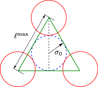
Refer to caption
Figure 7.3: In order to assure that the membrane cannot self-penetrate, one imposes a maximal length maxsuperscriptmax\ell^{\mathrm{max}} to the network’s bonds plus a hard-core potential between any two beads of the network. Here we show how max=23σ0superscriptmax23subscript𝜎0\ell^{\mathrm{max}}=2\sqrt{3}\,\sigma_{0} is obtained, with σ0subscript𝜎0\sigma_{0} the beads’ radius.

From 1990 on, the fluidity was taken into account by dynamically modifying the triangulation, while keeping the self-avoiding restrictions [137][138]. Since then, this model has been used in a wide variety of complex numerical experiments, such as studying the dynamics of vesicles and red blood cells in flows [139][140] and the budding of vesicles mediated by proteins [141]. As we explain in the next section, this well-established dynamical triangular network model was the basis for our numerical model of membrane.

7.2 Our numerical membrane

As shown in Fig. 7.1, we wanted to simulate a relatively large piece of weakly fluctuating membrane attached to a circular frame. Under these conditions, the probability of overhangs is very small and thus the probability that large fluctuations bring distant segments of the membrane into close spatial proximity is negligible. Consequently, in an approximation, we decided to ignore the hard-core potential between any two beads and consider only the interactions between neighboring beads, which is much less computer consuming. In this case, the meshwork phenomenological model presents a great advantage: with a mesh, we know at every instant which beads are neighbors, since they are attached by bonds, whereas in meshless models determining neighbors is not straightforward. So, we have decided to use a dynamically triangulated meshwork whose beads are phantom if they are not first neighbors.

In agreement with section 7.1, we denote the beads’ radius σ0subscript𝜎0\sigma_{0}. Each pair of neighboring beads interact through the potential

Vbond()={for<min,s(0)22formin<<max,for>max,subscript𝑉bondcasesforsuperscriptminmissing-subexpressionmissing-subexpressionmissing-subexpressionmissing-subexpressionmissing-subexpressionmissing-subexpressionmissing-subexpression𝑠superscriptsubscript022forsuperscriptminsuperscriptmaxmissing-subexpressionmissing-subexpressionmissing-subexpressionmissing-subexpressionmissing-subexpressionmissing-subexpressionmissing-subexpressionforsuperscriptmaxmissing-subexpressionmissing-subexpressionV_{\mathrm{bond}}(\ell)=\left\{\begin{array}[]{ccccc}\infty&$for$&\,\ell<\ell^{\mathrm{min}}\,,\\ \\ s\,\frac{(\ell-\ell_{0})^{2}}{2}&$for$&\,\ell^{\mathrm{min}}<\ell<\ell^{\mathrm{max}},\\ \\ \infty&$for$&\,\ell>\ell^{\mathrm{max}}\,,\end{array}\right. (7.1)

where \ell is the distance between the center of adjacent beads; min=2σ0superscriptmin2subscript𝜎0\ell^{\mathrm{min}}=2\,\sigma_{0} and max=23σ0superscriptmax23subscript𝜎0\ell^{\mathrm{max}}=2\sqrt{3}\,\sigma_{0} are, respectively, the minimal and maximal distance between the center of adjacent beads. The length 0subscript0\ell_{0} corresponds to a preferred distance that we have chosen as the average of the minimal and maximal allowed length: 0=(min+max)/2=(1+3)σ0subscript0superscriptminsuperscriptmax213subscript𝜎0\ell_{0}=(\ell^{\mathrm{min}}+\ell^{\mathrm{max}})/2=(1+\sqrt{3})\,\sigma_{0} (see Fig. 7.4).

Refer to caption
Figure 7.4: Potential between neighboring beads as a function of their distance \ell. The regions where the potential is \infty are shaded.

In section 1.3.6, we have seen that the bending rigidity of a weakly fluctuating membrane gives a contribution

Eκ=κ2Ap(2h)2𝑑Apsubscript𝐸𝜅𝜅2subscriptsubscript𝐴𝑝superscriptsuperscript22differential-dsubscript𝐴𝑝E_{\kappa}=\frac{\kappa}{2}\int_{A_{p}}(\nabla^{2}h)^{2}\,dA_{p}\, (7.2)

to the membrane’s energy. We will not consider topological changes in our simulation, so the Gaussian contribution to the curvature energy need not to be taken into account. In our network, we considered the commonly used bending energy discretization [128]

Eκdiscret=k2α,β|𝒏α𝒏β|2=kα,β(1𝒏α𝒏β),superscriptsubscript𝐸𝜅discret𝑘2subscript𝛼𝛽superscriptsubscript𝒏𝛼subscript𝒏𝛽2𝑘subscript𝛼𝛽1subscript𝒏𝛼subscript𝒏𝛽E_{\kappa}^{\mathrm{discret}}=\frac{k}{2}\sum_{\langle\alpha,\beta\rangle}|\bm{n}_{\alpha}-\bm{n}_{\beta}|^{2}=k\sum_{\langle\alpha,\beta\rangle}(1-\bm{n}_{\alpha}\cdot\bm{n}_{\beta})\,, (7.3)

where the sum runs over all pairs of adjacent triangles α𝛼\alpha and β𝛽\beta, with normal vectors 𝒏αsubscript𝒏𝛼\bm{n}_{\alpha} and 𝒏βsubscript𝒏𝛽\bm{n}_{\beta}, respectively. This discretization, however, presents a major problem: the relationship between κ𝜅\kappa and k𝑘k depends on the membrane’s geometry. Alternative more complex discretizations were proposed (see [129] for further details), but here we have chosen to keep this simplified discretization, since κ𝜅\kappa will be measured through the spectrum fluctuation. Note that eq.(7.3) is a good approximation only for 𝒏α𝒏βsubscript𝒏𝛼subscript𝒏𝛽\bm{n}_{\alpha}\approx\bm{n}_{\beta}. Indeed, for two triangles with 𝒏α=𝒏βsubscript𝒏𝛼subscript𝒏𝛽\bm{n}_{\alpha}=-\bm{n}_{\beta}, we have a contribution 2k2𝑘2\,k, while this configuration should be prohibitively costly.

At last, to impose a circular frame, each bead i𝑖i of the network’s boundary, shown in red in Fig. 7.5, is subject to a harmonic potential

Vfi=kf(RiRf)22,superscriptsubscript𝑉𝑓𝑖subscript𝑘fsuperscriptsubscript𝑅𝑖subscript𝑅𝑓22V_{f}^{i}=k_{\mathrm{f}}\,\frac{(R_{i}-R_{f})^{2}}{2}\,, (7.4)

where kfsubscript𝑘𝑓k_{f} is a constant that determines the rigidity of the potential, Risubscript𝑅𝑖R_{i} is the distance of the bead with respect to the center of the network and Rfsubscript𝑅𝑓R_{f} is the desired frame radius, imposed at the beginning of the simulation. Note that the projected area of the membrane Apsubscript𝐴𝑝A_{p} is not necessarily equivalent to πRf2𝜋superscriptsubscript𝑅𝑓2\pi R_{f}^{2}: it can vary more or less, depending on the choice of kfsubscript𝑘𝑓k_{f}.

To initialize the network, we construct a planar triangular network alternating lines with Nxsubscript𝑁𝑥N_{x} and Nx+1subscript𝑁𝑥1N_{x}+1 beads, up to Nxsubscript𝑁𝑥N_{x} lines. The beads are distanced by 0subscript0\ell_{0} and arranged as in Fig. 7.5.

Refer to caption
Figure 7.5: Initial configuration of the triangular network with Nx=5subscript𝑁𝑥5N_{x}=5. At this point, the network is planar and each bond measures 0subscript0\ell_{0}. The dashed circle represents the frame with Rf=6.96σ0subscript𝑅𝑓6.96subscript𝜎0R_{f}=6.96\,\sigma_{0} and Risubscript𝑅𝑖\vec{R}_{i} is the distance from a boundary bead to the center of the frame. The red large beads are subjected to the potential (7.4) in order to impose the circular frame. The ratio 0=(1+3)σ0subscript013subscript𝜎0\ell_{0}=(1+\sqrt{3})\sigma_{0} has not been taken into account in this graphical representation.

During the simulation, two kinds of moves were possible:

  1. 1.

    Move P: the position of one bead is modified. The beads shown in blue in Fig. 7.5 are free to move in three dimensions, while the ones belonging to the boundary can only move in the frame’s plane.

  2. 2.

    Move Flip: the network’s connectivity is changed in order to represent the membrane fluidity. This is done by eliminating an existing bond and proposing a new one, as shown in Fig. 7.6.
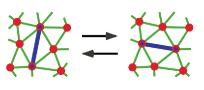
    Refer to caption
    Figure 7.6: Move called flip: a bond is deleted and a new one is proposed, changing the connectivity of the network.

In the following section, we will see how these moves were numerically implemented.

7.3 Simulation dynamics

As in section 2.3, we used a Monte Carlo method to generate a large sample of configurations. Again, the configurations were generated through a Markov chain algorithm: from a certain configuration ΩisubscriptΩ𝑖\Omega_{i}, a new configuration Ωi+1subscriptΩ𝑖1\Omega_{i+1} was accepted with a probability

P(ΩiΩi+1)=min[1,eβΔ],𝑃subscriptΩ𝑖subscriptΩ𝑖11superscript𝑒𝛽ΔP(\Omega_{i}\rightarrow\Omega_{i+1})=\min\left[1,e^{-\beta\,\Delta\mathcal{H}}\right]\,, (7.5)

where Δ=i+1iΔsubscript𝑖1subscript𝑖\Delta\mathcal{H}=\mathcal{H}_{i+1}-\mathcal{H}_{i} is the energy variation. In practice, we have

  1. 1.

    Move P: one particle i𝑖i is taken at random. If the particle belongs to the bulk of the network (blue beads in Fig. 7.5), we propose a new position 𝒓i=𝒓i+Δ𝒓superscriptsubscript𝒓𝑖subscript𝒓𝑖Δ𝒓\bm{r}_{i}^{\prime}=\bm{r}_{i}+\Delta\bm{r}, where Δ𝒓=δr×[rand(1,1)𝒆x+rand(1,1)𝒆y+rand(1,1)𝒆z]Δ𝒓𝛿𝑟delimited-[]rand11subscript𝒆𝑥rand11subscript𝒆𝑦rand11subscript𝒆𝑧\Delta\bm{r}=\delta r\times[\mathrm{rand}(-1,1)\,\bm{e}_{x}+\mathrm{rand}(-1,1)\,\bm{e}_{y}+\mathrm{rand}(-1,1)\,\bm{e}_{z}] , with rand(a,b)rand𝑎𝑏\mathrm{rand}(a,b) a random number between a𝑎a and b𝑏b, 𝒆zsubscript𝒆𝑧\bm{e}_{z} the direction perpendicular to the frame’s plane and 𝒆xsubscript𝒆𝑥\bm{e}_{x}, 𝒆ysubscript𝒆𝑦\bm{e}_{y} two perpendicular directions contained in the frame’s plane. Each bond attached to the particle i𝑖i has its length modified. The normal, area and projected area of all triangles that have the particle i𝑖i as a vertex must also be re-evaluated. The energy variation has thus two contributions: one coming from the changing on the bond’s length and other coming from the curvature. We can see a representation of them in Fig. 7.7.

    In the case of a boundary bead (red large beads in Fig. 7.5), one has simply Δ𝒓=δr×[rand(1,1)𝒆x+rand(1,1)𝒆y]Δ𝒓𝛿𝑟delimited-[]rand11subscript𝒆𝑥rand11subscript𝒆𝑦\Delta\bm{r}=\delta r\times[\mathrm{rand}(-1,1)\,\bm{e}_{x}+\mathrm{rand}(-1,1)\,\bm{e}_{y}]. In addition to the former contributions, one needs also in this case to consider the energy variation coming from the frame’s potential. The value of δr𝛿𝑟\delta r was adjusted to have an acceptance rate of 50%similar-toabsentpercent50\sim 50\%.

    Refer to caption
    (a) Bonds’ contribution.
    Refer to caption
    (b) Curvature contribution.
    Figure 7.7: Contributions to the energy variation when the position of a bead, here shown in blue, is modified. At left, we represent the energy variation due to the modification of the length of each tether attached to the bead. At right, we represent the curvature contribution: the normal (segment at the center of the triangles shown in green), area and projected area of the triangles that have the blue bead as a vertex (dark violet triangles) must be re-evaluated. One must subsequently consider the variation of the curvature energy between all adjacent violet triangles.
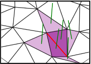
    Refer to caption
    (a) Before the flip.
    Refer to caption
    (b) After the flip.
    Figure 7.8: Energy variation for a typical flip move. The red bond represents the bond that is suppressed (at left) / created (at right). The energy variation is due to the construction of a new bond of different length and to the modification of the normals (segment at the center of the triangles shown in green) of the dark violet triangles. Consequently, one has to consider the variation of the curvature energy between the dark violet triangles and their neighbors, shown in light violet.
  2. 2.

    Move Flip: we randomly choose a bond belonging to the network’s bulk. We propose a substitution to this bond, as shown in Fig. 7.6. The normal, area and projected area of the two new triangles is calculated and the total energy variation involves the terms illustrated in Fig. 7.8. Remark that the frame potential never contributes to this kind of move, since the position of the beads remain constant.

    Note also that the acceptance rate of flip moves is completely determined by the tension applied to the network through the choice of Rfsubscript𝑅𝑓R_{f} and by the choice of the constants s𝑠s and k𝑘k. Typically, we have an acceptance rate between 1%percent11\% and 10%percent1010\%, depending on the chosen values. For very large tensions, this can be a serious issue, since the energy variation ΔΔ\Delta\mathcal{H} is in general very large. Consequently, almost no flip is accepted and the network does not mimic the membrane’s fluidity.

In both kinds of move, one has to re-evaluate the normal, area and projected area of some triangles. For each triangle, we evaluate the cross product of two of its edges to obtain the direction of its normal and its new area. One must however pay attention to the order in which the cross product is evaluated to assure that the orientation of the normal is correct. Similarly, to obtain the new projected area, we considered the cross product of the projection of two of the triangle’s edges onto the frame’s plane.
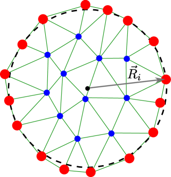
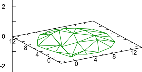
Refer to caption
(a) Top view.
Refer to caption
(b) Side view.
Figure 7.9: Configuration for a small network with Nx=5subscript𝑁𝑥5N_{x}=5 and a total of N=27𝑁27N=27 beads, βσ02s=1𝛽superscriptsubscript𝜎02𝑠1\beta\,\sigma_{0}^{2}\,s=1, βk=10𝛽𝑘10\beta\,k=10, βσ02kf=30𝛽superscriptsubscript𝜎02subscript𝑘𝑓30\beta\,\sigma_{0}^{2}\,k_{f}=30 and Rf=6.96σ0subscript𝑅𝑓6.96subscript𝜎0R_{f}=6.96\,\sigma_{0} after the first 2×1042superscript1042\times 10^{4} Monte Carlo steps. In the top view, we see that the boundaries roughly coincide with the imposed circular frame after Nneg=2×10⁴subscript𝑁neg2superscript104N_{\mathrm{neg}}=2\times 10^{4} steps (the center of the frame is indicated by the black dot). Observe also that the topology of the network has changed: one finds beads with five and seven neighbors. In the side view, we can see that the membrane fluctuates around the plane (note that the vertical and the horizontal scales are different).

For each attempt of move P𝑃P, we try a flip. We call a Monte Carlo step a set of N𝑁N sequences of a move P followed by a move flip, with N𝑁N the number of beads. The first Nnegsubscript𝑁negN_{\mathrm{neg}} steps are not taken into account in the evaluation of averages to assure that the membrane has reached equilibrium. In Fig. 7.9, we show the configuration of a small network after Nneg=2×10⁴subscript𝑁neg2superscript104N_{\mathrm{neg}}=2\times 10^{4} Monte Carlo steps. The frame is already roughly circular (the fit with the frame depends on the choice of kfsubscript𝑘𝑓k_{f}). We will call a complete sequence of Nnegsubscript𝑁negN_{\mathrm{neg}} Monte Carlo steps followed by a number of equilibrium Monte Carlo steps Nitersubscript𝑁iterN_{\mathrm{iter}} a run.

Refer to caption
Figure 7.10: Snapshots of the network at every 2×1042superscript1042\times 10^{4} Monte Carlo steps. The height of the membrane is represented by the shading scale at right and the three spatial coordinates are measured in unities of σ0subscript𝜎0\sigma_{0}. This image was obtained using the interpolation explained in the following (section 7.4.2) for Ngrid=128subscript𝑁grid128N_{\mathrm{grid}}=128. Remark that the membrane weakly departs from the plane and that the configurations look uncorrelated after 2×1042superscript1042\times 10^{4} iterations.
7.3.1 Verifications and equilibration criteria

In order to obtain meaningful averages, we have to assure that our configuration sampling is reasonably uniform over the space of the possible configurations, i. e, we have to assure that Nitersubscript𝑁iterN_{\mathrm{iter}} is large enough. We have not done a systematic study on how the equilibration time depends on the network’s size and constants at this preliminary stage. We have rather evaluated the equilibration at each run. In the following, we exemplify how we have carried this out using a typical network with 410410410 beads (Nx=10subscript𝑁𝑥10N_{x}=10), βk=5𝛽𝑘5\beta\,k=5, βσ02kf=10𝛽superscriptsubscript𝜎02subscript𝑘𝑓10\beta\,\sigma_{0}^{2}\,k_{f}=10, βσ02s=1𝛽superscriptsubscript𝜎02𝑠1\beta\,\sigma_{0}^{2}\,s=1 and Rf=33.04σ0subscript𝑅𝑓33.04subscript𝜎0R_{f}=33.04\,\sigma_{0}. We assume that the system has already relaxed to its equilibrium state after Nnegsubscript𝑁negN_{\mathrm{neg}} Monte Carlo steps. First of all, we have evaluated visually the system’s evolution, as shown in Fig. 7.10. We can see that in this case, the configurations are already very different after 2×1042superscript1042\times 10^{4} Monte Carlo steps.

Visually, we have also checked if all the bonds were being flipped with a similar frequency. For the same network as before, we show in Fig. 7.11(a) a map of the bonds colored as a function of the relative frequency with which they were flipped. We can see that the coloring is very uniform, indicating that the network does not present regions with different liquidity. As a supplementary check, we have also studied the diffusion of one bead over time (see Fig. 7.11(b)).
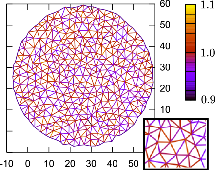
Refer to caption
(a) Flip frequency.
Refer to caption
(b) Diffusion of one bead.
Figure 7.11: At left, we see the top view of the network after 2×1052superscript1052\times 10^{5} iterations. The inset shows a detail of the network. Each bond was colored with the relative frequency with which flips were accepted (the average was normalized to one). We see that flips happened uniformly in space. At right, the diffusion of a bead after the same number of iterations testify of the membrane’s liquidity (red curve). We have superposed a network snapshot (in green) for comparison.

On a second moment, we have studied the spatial average of the membrane’s height: since there is no asymmetry, after a sufficiently large number of steps, one should expect this quantity to vanish. This condition is however not sufficient, since the membrane can have a vanishing spatial average and be non-planar. We have thus monitored the local average of the membrane’s height, i. e., we have studied the average shape of the membrane (see Fig. 7.12). In practice, this was done by constructing an interpolation that will be explained in section 7.4.2 and averaging the height over each cell of the interpolation grid.
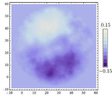
Refer to caption
Figure 7.12: Average shape of the membrane after 2×1062superscript1062\times 10^{6} Monte Carlo steps. The average height of the membrane is represented by the shading scale at right and the three spatial coordinates are measured in unities of σ0subscript𝜎0\sigma_{0}. Once again, we have used Ngrid=128subscript𝑁grid128N_{\mathrm{grid}}=128 to construct an interpolation grid. Note that the vertical scale is far smaller than the horizontal. The parameters are the same as in the last figures.

Finally, we have monitored the evolution of longest Fourier modes h1,0subscript10h_{1,0}, h0,1subscript01h_{0,1} and h1,1subscript11h_{1,1} (in the next section we explain how we have obtained the Fourier decomposition). Typical curves can be seen in Fig. 7.13. We can see that after 104absentsuperscript104\approx 10^{4} steps, the coefficients are uncorrelated, which means that the longest modes have relaxed. Accordingly, we have considered that in this case, 2×1062superscript1062\times 10^{6} steps generated a sufficiently large sampling of the configuration space.
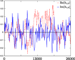
Refer to caption
(a) Mode h1,0subscript10h_{1,0}.
Refer to caption
(b) Mode h0,1subscript01h_{0,1}.
Refer to caption
(c) Mode h1,1subscript11h_{1,1}.
Figure 7.13: Fourier coefficients as a function of the number of Monte Carlo steps. The parameters of the network are the same as before.

7.4 Measuring tensions and the excess area

In this section we describe how we measured the effective tension τ𝜏\tau and the excess area α𝛼\alpha. We explain also the algorithm used to derive the fluctuation spectrum, from whose average we could derive κ𝜅\kappa and the tension r𝑟r. Finally, we discuss the internal tension σ𝜎\sigma in section 7.4.3.

7.4.1 Excess area and mechanical tension measures

In order to obtain τ𝜏\tau, we study the total force that the harmonic potential given in eq.(7.4) exerts over the beads at the network’s boundary, which represents the force applied by the frame onto the membrane:

f=kfi(RiRf),𝑓subscript𝑘𝑓subscript𝑖subscript𝑅𝑖subscript𝑅𝑓f=-k_{f}\sum_{i}(R_{i}-R_{f})\,, (7.6)

where the sum runs over the beads at the network’s edge and Risubscript𝑅𝑖R_{i} is their distance to the center of the frame. For kfsubscript𝑘𝑓k_{f} large enough, the edge of the network fits well with the frame with radius Rfsubscript𝑅𝑓R_{f} and thus the effective tension of a configuration is given by

τi=f2πRf.subscript𝜏𝑖𝑓2𝜋subscript𝑅𝑓\tau_{i}=\frac{f}{2\pi R_{f}}\,. (7.7)

During a run, τisubscript𝜏𝑖\tau_{i} was evaluated at the end of each Monte Carlo step. At the end of it, we obtained τ=τi𝜏delimited-⟨⟩subscript𝜏𝑖\tau=\langle\tau_{i}\rangle and its standard deviation (Δτ)2=τi2τi2superscriptΔ𝜏2delimited-⟨⟩superscriptsubscript𝜏𝑖2superscriptdelimited-⟨⟩subscript𝜏𝑖2(\Delta\tau)^{2}=\langle\tau_{i}^{2}\rangle-\langle\tau_{i}\rangle^{2}.

Concerning the excess area, we carefully updated the membrane’s projected area Apsubscript𝐴𝑝A_{p} and actual area A𝐴A after each attempt of move. At the end of each Monte Carlo step, the excess area of the configuration

αi=AApApsubscript𝛼𝑖𝐴subscript𝐴𝑝subscript𝐴𝑝\alpha_{i}=\frac{A-A_{p}}{A_{p}}\, (7.8)

was added to a variable in order to obtain α=αi𝛼delimited-⟨⟩subscript𝛼𝑖\alpha=\langle\alpha_{i}\rangle in the end of the run.

7.4.2 Fluctuation spectrum

Let’s consider a square piece of membrane with lateral size L𝐿L weakly departing from a plane, whose shape is described in the Monge’s gauge by h(𝒓)𝒓h(\bm{r}). In terms of Fourier modes, h(𝒓)𝒓h(\bm{r}) can be written as

h(𝒓)=𝒒hn,mei𝒒𝒓,𝒓subscript𝒒subscript𝑛𝑚superscript𝑒𝑖𝒒𝒓h(\bm{r})=\sum_{\bm{q}}h_{n,m}\,e^{i\,\bm{q}\cdot\bm{r}}\,, (7.9)

with 𝒓=x𝒆x+y𝒆y𝒓𝑥subscript𝒆𝑥𝑦subscript𝒆𝑦\bm{r}=x\,\bm{e}_{x}+y\,\bm{e}_{y}, 𝒒=2π/L(n,m)𝒒2𝜋𝐿𝑛𝑚\bm{q}=2\pi/L\,(n,m), n,m𝑛𝑚n,m\in\mathbb{N} and

𝒒|n|Nmax|m|Nmax,subscript𝒒subscript𝑛subscript𝑁maxsubscript𝑚subscript𝑁max\sum_{\bm{q}}\equiv\sum_{|n|\leq N_{\mathrm{max}}}\sum_{|m|\leq N_{\mathrm{max}}}\,, (7.10)

where Nmax=L/(2a)subscript𝑁max𝐿2𝑎N_{\mathrm{max}}=L/(2a) corresponds to the smallest possible wave length. Note that here we have used a slightly different normalization from the rest of this work. The coefficients hn,msubscript𝑛𝑚h_{n,m} are in general complex and hn,m=hn,msubscript𝑛𝑚superscriptsubscript𝑛𝑚h_{-n,-m}=h_{n,m}^{*}, where the superscript * stands for the complex conjugate. It is given by

hn,m=1L20L0Lh(𝒓)ei𝒒𝒓𝑑𝒓.subscript𝑛𝑚1superscript𝐿2superscriptsubscript0𝐿superscriptsubscript0𝐿𝒓superscript𝑒𝑖𝒒𝒓differential-d𝒓h_{n,m}=\frac{1}{L^{2}}\int_{0}^{L}\int_{0}^{L}h(\bm{r})\,e^{-i\,\bm{q}\cdot\bm{r}}\,d\bm{r}\,. (7.11)

In section 1.3.6, we have seen that membranes connected to a lipid reservoir could have their energy described by the Helfrich Hamiltonian (eq.(1.15)). Accordingly, the average of the Fourier coefficients respects

|hn,m|2=1L2kBTrq2+κq4,delimited-⟨⟩superscriptsubscript𝑛𝑚21superscript𝐿2subscript𝑘B𝑇𝑟superscript𝑞2𝜅superscript𝑞4\langle|h_{n,m}|^{2}\rangle=\frac{1}{L^{2}}\,\frac{k_{\mathrm{B}}T}{rq^{2}+\kappa q^{4}}\,, (7.12)

where r𝑟r is the macroscopic counterpart of the internal tension σ𝜎\sigma and κ𝜅\kappa is the bending rigidity (in fact, as discussed before in section 1.3.6, it corresponds more precisely to an effective bending rigidity due to renormalization effects). As in laboratory experiments, we would like to measure the fluctuation spectrum of our numerical membrane in order to derive r𝑟r and κ𝜅\kappa. In the following, we will explain how it was done.

Obtaining the fluctuation spectrum

For a general wave-vector (n,m)𝑛𝑚(n,m), we have to evaluate eq.(7.11) in order to obtain hn,msubscript𝑛𝑚h_{n,m}. The first numerical difficulty comes from the fact that instead of a continuous surface h(𝒓)𝒓h(\bm{r}), we have access only to the position and height of the beads. Consequently, the first step is to built an approximation to the network’s surface by discretizing it over a square grid of Ngrid×Ngridsubscript𝑁gridsubscript𝑁gridN_{\mathrm{grid}}\times N_{\mathrm{grid}} cells with lateral side L𝐿L, as exemplified in Fig. 7.14. Each cell of has a lateral size Δ=L/NgridΔ𝐿subscript𝑁grid\Delta=L/N_{\mathrm{grid}}. We choose L𝐿L slightly bigger than 2Rf2subscript𝑅𝑓2\,R_{f} to avoid problems with the discontinuities at the edges of the grid.
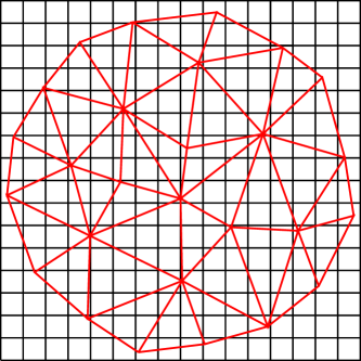
Refer to caption
Figure 7.14: Top view of a network with Nx=5subscript𝑁𝑥5N_{x}=5 and a total of N=27𝑁27N=27 beads (red). To evaluate the coefficients of the Fourier transform, we discretized the membrane over the grid shown in black (Ngrid=16subscript𝑁grid16N_{\mathrm{grid}}=16 here).

The discretized version of eq.(7.11), known as DFT (Discrete Fourier Transform) is given by

hn,m=1Ngrid2α=0Ngrid1β=0Ngrid1hα,βe2πi(nα+mβ)Ngrid,subscript𝑛𝑚1superscriptsubscript𝑁grid2superscriptsubscript𝛼0subscript𝑁grid1superscriptsubscript𝛽0subscript𝑁grid1subscript𝛼𝛽superscript𝑒2𝜋𝑖𝑛𝛼𝑚𝛽subscript𝑁gridh_{n,m}=\frac{1}{N_{\mathrm{grid}}^{2}}\sum_{\alpha=0}^{N_{\mathrm{grid}}-1}\sum_{\beta=0}^{N_{\mathrm{grid}}-1}h_{\alpha,\beta}\,e^{2\pi i\,\frac{(n\alpha+m\beta)}{N_{\mathrm{grid}}}}\,, (7.13)

where hα,βsubscript𝛼𝛽h_{\alpha,\beta} is the height of the cell whose bottom left corner position is 𝒓=Δ×(α,β)𝒓Δ𝛼𝛽\bm{r}=\Delta\times(\alpha,\beta). At this point, we need to attribute a height to each cell of the grid, which is initially set to zero. We do so in two steps:

  • First, we obtain the plane’s equation for each triangle from the position of its three vertex. Using this equation, we evaluate the height of some points inside the triangle, as shown in Fig. 7.15.
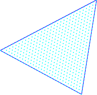
    Refer to caption
    (a) Top view.
    Refer to caption
    (b) Side view.
    Figure 7.15: Initially, we know only the position of the triangle’s vertex. From them, the plane’s equation is obtained and the height is evaluated over each dot on the triangle.
  • Secondly, the cell that contains the projection of a dot receives its height. If the projection of more than one dot falls inside the same cell, we attribute the average of the their height to the cell (see Fig. 7.16).
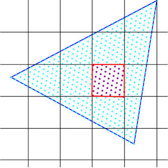
    Refer to caption
    Figure 7.16: To evaluate the height of the cell shown in red, we averaged the height of the dots whose projection are shown in violet.

Fig. 7.17 shows an example to testify of the quality of our approximation.
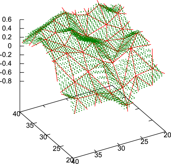
Refer to caption
Figure 7.17: Piece of a network with Nx=10subscript𝑁𝑥10N_{x}=10 (N=410𝑁410N=410 beads) and Ngrid=128subscript𝑁grid128N_{\mathrm{grid}}=128, shown in red. The green dots correspond to the height of each cell of the grid, obtained through the method explained above. Remark the good quality of the approximation procedure. Note that the vertical scale is different from the horizontal.

Once the approximative grid is built, we can evaluate eq.(7.13) which has a great advantage: it can be evaluated using the FFT (Fast Fourier Transform) algorithm with a Ngrid2log(Ngrid)superscriptsubscript𝑁grid2subscript𝑁gridN_{\mathrm{grid}}^{2}\log(N_{\mathrm{grid}}) complexity, instead of a Ngrid4superscriptsubscript𝑁grid4N_{\mathrm{grid}}^{4} complexity for naive algorithms. We used thus the cdft (complex discrete Fourier transform) routine of the FFT library implemented by Takuya Ooura [142], which is a general library to evaluate FFT under the condition that Ngridsubscript𝑁gridN_{\mathrm{grid}} is a power of 222.

A subtlety

The prediction given in eq.(7.12) is valid for a squared piece of membrane with lateral size L𝐿L. Since our membrane is round, our situation corresponds to a squared membrane seen through a circular mask, given by

circ(𝒓)={1forr<Rf,0forr>Rf.circ𝒓cases1for𝑟subscript𝑅𝑓missing-subexpressionmissing-subexpressionmissing-subexpressionmissing-subexpressionmissing-subexpressionmissing-subexpressionmissing-subexpression0for𝑟subscript𝑅𝑓missing-subexpressionmissing-subexpression\mathrm{circ}(\bm{r})=\left\{\begin{array}[]{ccccc}1&$for$&\,r<R_{f}\,,\\ \\ 0&$for$&\,r>R_{f}\ .\end{array}\right. (7.14)

So, we are actually performing numerically the Fourier transform of the function h(𝒓)𝒓h(\bm{r}) that denotes the height of the membrane multiplied by circ(𝒓)circ𝒓\mathrm{circ}(\bm{r}), instead of just performing the Fourier transform of h(𝒓)𝒓h(\bm{r}). Indicating the Fourier transform by a superscript ^^absent\,\hat{}\,, we recall the convolution theorem:

(hcirc)^=h^circ^,^circ^^circ\widehat{(h\,\,\mathrm{circ})}=\hat{h}*\widehat{\mathrm{circ}}\,, (7.15)

where * indicates the convolution between the two functions.

In order to obtain h^^\hat{h}, we will evaluate the Fourier transform of circ(𝒓)circ𝒓\mathrm{circ}(\bm{r}). Using the above presented definition, we have [143]

circ^^circ\displaystyle\widehat{\mathrm{circ}} =\displaystyle= 1L20L0Lcirc(𝒓)ei𝒒𝒓𝑑𝒓,1superscript𝐿2superscriptsubscript0𝐿superscriptsubscript0𝐿circ𝒓superscript𝑒𝑖𝒒𝒓differential-d𝒓\displaystyle\frac{1}{L^{2}}\int_{0}^{L}\int_{0}^{L}\mathrm{circ}(\bm{r})\,e^{-i\,\bm{q}\cdot\bm{r}}\,d\bm{r}\,, (7.16)
=\displaystyle= 1L20Rfrcirc(𝒓)(02πei𝒒𝒓𝑑θ)𝑑r,1superscript𝐿2superscriptsubscript0subscript𝑅𝑓𝑟circ𝒓superscriptsubscript02𝜋superscript𝑒𝑖𝒒𝒓differential-d𝜃differential-d𝑟\displaystyle\frac{1}{L^{2}}\int_{0}^{R_{f}}r\,\mathrm{circ}(\bm{r})\left(\int_{0}^{2\pi}e^{-i\,\bm{q}\cdot\bm{r}}d\theta\right)\,dr\,,
=\displaystyle= 2πL20RfrJ0(qr)𝑑r,2𝜋superscript𝐿2superscriptsubscript0subscript𝑅𝑓𝑟subscript𝐽0𝑞𝑟differential-d𝑟\displaystyle\frac{2\pi}{L^{2}}\int_{0}^{R_{f}}r\,J_{0}(q\,r)\,dr\,,
similar-to-or-equals\displaystyle\simeq π2RfJ1(qRf)q,𝜋2subscript𝑅𝑓subscript𝐽1𝑞subscript𝑅𝑓𝑞\displaystyle\frac{\pi}{2\,R_{f}}\,\frac{J_{1}(q\,R_{f})}{q}\,,

where Jisubscript𝐽𝑖J_{i} is the Bessel function of order i𝑖i. In the last passage, we have used the fact that L2Rf𝐿2subscript𝑅𝑓L\approx 2\,R_{f}. This function has a very marked pike, as shown in Fig. 7.18.
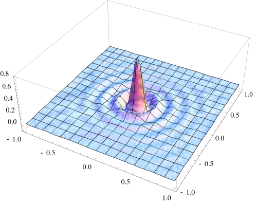
Refer to caption
Figure 7.18: Plot of circ^^circ\widehat{\mathrm{circ}} as a function of the wave-vector q𝑞q for Rf=32σ0subscript𝑅𝑓32subscript𝜎0R_{f}=32\,\sigma_{0}. Note that the function presents a very marked pike.

From eq.(7.15), since circ^^circ\widehat{\mathrm{circ}} is so piked, we have

(hcirc)^^circ\displaystyle\widehat{(h\,\mathrm{circ})} similar-to-or-equals\displaystyle\simeq h^×circ^(0),^^circ0\displaystyle\hat{h}\times\widehat{\mathrm{circ}}(0)\,, (7.17)
similar-to-or-equals\displaystyle\simeq h^×π4.^𝜋4\displaystyle\hat{h}\times\frac{\pi}{4}\,.

Finally, to obtain the Fourier transform of h(𝒓)𝒓h(\bm{r}), we have to multiply the Fourier coefficients h~n,msubscript~𝑛𝑚\tilde{h}_{n,m} obtained numerically (considering the mask) by 4/π4𝜋4/\pi:

hn,m=4πh~n,m.subscript𝑛𝑚4𝜋subscript~𝑛𝑚h_{n,m}=\frac{4}{\pi}\,\tilde{h}_{n,m}\,. (7.18)

In the following, we will keep the notation h~n,msubscript~𝑛𝑚\tilde{h}_{n,m} for the coefficients obtained with the mask.

During a run

As the process of grid construction is relatively computer consuming, the fluctuation spectrum was measured over Nspecsubscript𝑁specN_{\mathrm{spec}} configurations uniformly spaced during a run. At each time, we obtained the Re(h~n,m)Resubscript~𝑛𝑚\mathrm{Re}(\tilde{h}_{n,m}) and Im(h~n,m)Imsubscript~𝑛𝑚\mathrm{Im}(\tilde{h}_{n,m}), i. e., the real and complex parts of each Fourier coefficient, with |n|Ngrid𝑛subscript𝑁grid|n|\leq N_{\mathrm{grid}} and |m|Ngrid𝑚subscript𝑁grid|m|\leq N_{\mathrm{grid}}. In the end of the run, we evaluated |h~n,m|2=Re(h~n,m)2+Im(h~n,m)2delimited-⟨⟩superscriptsubscript~𝑛𝑚2delimited-⟨⟩Resuperscriptsubscript~𝑛𝑚2delimited-⟨⟩Imsuperscriptsubscript~𝑛𝑚2\langle|\tilde{h}_{n,m}|^{2}\rangle=\langle\mathrm{Re}(\tilde{h}_{n,m})^{2}\rangle+\langle\mathrm{Im}(\tilde{h}_{n,m})^{2}\rangle.

We plotted then 1/(q2L2|hn,m|2)1superscript𝑞2superscript𝐿2delimited-⟨⟩superscriptsubscript𝑛𝑚21/(q^{2}L^{2}\langle|h_{n,m}|^{2}\rangle) as a function of q2superscript𝑞2q^{2}, with q2=(4π2)/(L2)(n2+m2)superscript𝑞24superscript𝜋2superscript𝐿2superscript𝑛2superscript𝑚2q^{2}=(4\pi^{2})/(L^{2})\,(n^{2}+m^{2}) and hnm=4/πh~n,msubscript𝑛𝑚4𝜋subscript~𝑛𝑚h_{nm}=4/\pi\,\tilde{h}_{n,m}. From eq.(7.11), we expect, at least for large wave-lengths, a linear relation between these quantities: from the y𝑦y-intercept of the curve, we derive r𝑟r, while from it’s slope we obtain κ𝜅\kappa. In Fig. 7.19, we show an example such a plot with a linear fit to the region of large wave-lengths.

7.4.3 Internal tension 𝝈𝝈\bm{\sigma}

As discussed in section 1.3.5, the internal tension σ𝜎\sigma is the energetic cost associated to an unitary increase in the microscopical area A𝐴A of the membrane. From the energy E𝐸E of a system, it can be obtained through:

σ=(EA).𝜎𝐸𝐴\sigma=\left(\frac{\partial E}{\partial A}\right)\,. (7.19)

Let’s consider a general triangle in the bulk of our meshwork. In an approximation, let’s consider that the triangle is equilateral and has \ell as lateral size. From eq.(7.1), the local energy Etrisubscript𝐸triE_{\mathrm{tri}} associated to this triangle is given by

Etri=3×12×s(0)22+Ecurv,subscript𝐸tri312𝑠superscriptsubscript022subscript𝐸curvE_{\mathrm{tri}}=3\times\frac{1}{2}\times s\,\frac{(\ell-\ell_{0})^{2}}{2}+E_{\mathrm{curv}}\,, (7.20)

where Ecurvsubscript𝐸curvE_{\mathrm{curv}} is a contribution coming from the bending rigidity. The factor 333 comes from the three sides of the triangle, while the term 1/2121/2 comes from the fact that each side is shared by two adjacent triangles. Note that the first term is the only contribution involving the bead-to-bead distance \ell. Under the assumption that the triangle is equilateral, its area is given by

Atri=342.subscript𝐴tri34superscript2A_{\mathrm{tri}}=\frac{\sqrt{3}}{4}\,\ell^{2}\,. (7.21)

From eq.(7.19) and under the assumption of an equilateral triangle, we can define a local internal tension:

σlocsubscript𝜎loc\displaystyle\sigma_{\mathrm{loc}} =\displaystyle= (EtriAtri),subscript𝐸trisubscript𝐴tri\displaystyle\left(\frac{\partial E_{\mathrm{tri}}}{\partial A_{\mathrm{tri}}}\right)\,, (7.22)
=\displaystyle= (Etri)(Atri)1,subscript𝐸trisuperscriptsubscript𝐴tri1\displaystyle\left(\frac{\partial E_{\mathrm{tri}}}{\partial\ell}\right)\,\left(\frac{\partial A_{\mathrm{tri}}}{\partial\ell}\right)^{-1}\,,
=\displaystyle= 3s0.3𝑠subscript0\displaystyle\sqrt{3}\,s\,\frac{\ell-\ell_{0}}{\ell}\,.

Now, in our simulation, the sides of all triangles are submitted to the same harmonic potential given in eq.(7.1). Accordingly, the hypothesis that each triangle is in average equilateral is very reasonable. Moreover, as the system is spatially uniform, we propose thus a generalization of eq.(7.22) as a estimate of the internal tension:

σ=3s¯0¯,𝜎3𝑠delimited-⟨⟩¯subscript0delimited-⟨⟩¯\sigma=\sqrt{3}\,s\,\frac{\langle\bar{\ell}\rangle-\ell_{0}}{\langle\bar{\ell}\rangle}\,, (7.23)

where the bar over \ell indicates the spatial average of the bead-to-bead distance, while \langle\rangle indicates as usually the average over an ensemble of configurations.

In practice, we have kept track of the average length of the bonds over the network ¯¯\bar{\ell} at each Monte Carlo step. At the end of the run, we could thus evaluate the average of ¯¯\bar{\ell} over a the ensemble of configurations to obtain σ𝜎\sigma.

7.5 Some first results

The results presented here consist of a preliminary set of runs for a network with Nx=10subscript𝑁𝑥10N_{x}=10, with a total of N=410𝑁410N=410 beads. We have kept the parameters βk=5𝛽𝑘5\beta\,k=5, βσ02kf=10𝛽superscriptsubscript𝜎02subscript𝑘𝑓10\beta\,\sigma_{0}^{2}\,k_{f}=10 and βσ02s=1𝛽superscriptsubscript𝜎02𝑠1\beta\,\sigma_{0}^{2}\,s=1. As discussed in section 7.3.1, we let the system evolve during Nneg=104subscript𝑁negsuperscript104N_{\mathrm{neg}}=10^{4} steps in order to assure that the final frame shape had been attained. The averages were made in a second time, over Niter=2×10⁶subscript𝑁iter2superscript106N_{\mathrm{iter}}=2\times 10^{6} steps during which 150015001500 spectra were evaluated.

We performed fifteen runs with these parameters, increasing at each run the membrane’s tension by widening the frame’s radius: the initial radius Rf=32.34σ0subscript𝑅𝑓32.34subscript𝜎0R_{f}=32.34\,\sigma_{0} was successively increased of 0.35σ00.35subscript𝜎00.35\,\sigma_{0} up to Rf=37.39σ0subscript𝑅𝑓37.39subscript𝜎0R_{f}=37.39\,\sigma_{0}. As the radius increased, the excess area decreased from 3.3%absentpercent3.3\approx 3.3\% to 2.4%absentpercent2.4\approx 2.4\%.

For each run, we have plotted the fluctuation spectrum as detailed in section 7.4.2 to obtain r𝑟r and κ𝜅\kappa. A typical example is shown in Fig. 7.19, where we have colored the points in function of the angle that the wave-vector associated to the mode did with the horizontal direction of the grid. First, we can remark that there is no clear color pattern, which indicates that the membrane is indeed isotropic. Second, we can see that in the region of large wave-lengths, the dots are well-fitted by a linear curve, from which we deduce r𝑟r and κ𝜅\kappa.

Refer to caption
Figure 7.19: Deducing r𝑟r and κ𝜅\kappa: the colored dots represent the inverse of the average intensity of a mode plotted as a function of the squared wave vector. The colored scale represents the angle that the wave-vector does with the horizontal direction of the grid. Remark that there is no color pattern, which is an evidence of the system’s isotropy. The line represents the linear fit for large wave lengths (λ>9σ0𝜆9subscript𝜎0\lambda>9\,\sigma_{0}, corresponding to q2<0.5superscript𝑞20.5q^{2}<0.5) from which r𝑟r and κ𝜅\kappa are deduced.

We plot the results obtained for each run as a function of the corresponding excess area in Fig. 7.20 (we remind that the smaller the excess area, the bigger the frame’s radius). In Fig. 7.20(a), we note a small dependence of κ𝜅\kappa as a function of the excess area. In Fig. 7.20(b), we compare the values of τ𝜏\tau, σ𝜎\sigma and r𝑟r: the three decrease as the excess area increases, as expected. As we predict, we have always σ𝜎\sigma bigger than τ𝜏\tau and their difference is bigger for small tensions. Concerning the renormalized tension r𝑟r, we find values not very different from τ𝜏\tau and σ𝜎\sigma, which is reassuring. The tension fluctuation ΔτΔ𝜏\Delta\tau, represented by red bars, seems almost constant, which agrees at least qualitatively with the predictions of chapter 3.
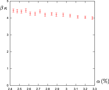
Refer to caption
(a) Bending rigidity.
Refer to caption
(b) Tensions.
Figure 7.20: At left: values of κ𝜅\kappa in units of kBTsubscript𝑘B𝑇k_{\mathrm{B}}T obtained by the linear fit shown in Fig. 7.19 for different values of excess area. At right: measured tensions as a function of the excess area.

At this point, we have good indications that the our network mimics well a liquid membrane under the Helfrich Hamiltonian. In the next section, we will test quantitatively the compatibility of these results with our theoretical predictions.

7.5.1 Difference between 𝝉𝝉\bm{\tau}, 𝝈𝝈\bm{\sigma} and 𝒓𝒓\bm{r} and our predictions

In chapter 2, we predicted that

τ=σkBTΛ28π[1σσrln(1+σrσ)],𝜏𝜎subscript𝑘B𝑇superscriptΛ28𝜋delimited-[]1𝜎subscript𝜎𝑟1subscript𝜎𝑟𝜎\tau=\sigma-\frac{k_{\mathrm{B}}T\,\Lambda^{2}}{8\pi}\left[1-\frac{\sigma}{\sigma_{r}}\ln\left(1+\frac{\sigma_{r}}{\sigma}\right)\right]\,, (7.24)

where ΛΛ\Lambda is the bigger wave-vector possible and σr=κΛ2subscript𝜎𝑟𝜅superscriptΛ2\sigma_{r}=\kappa\Lambda^{2}.

In this section, we would like to verify quantitatively the compatibility of eq.(7.24) with the data of the last section. We made a one-variable fit of eq.(7.24) by adjusting the value of ΛΛ\Lambda. The best fit, for Λ=1.03σ01Λ1.03superscriptsubscript𝜎01\Lambda=1.03\,\sigma_{0}^{-1}, is shown in Fig. 7.21(a). The compatibility between the data obtained from the simulation and the predicted values is relatively poor.
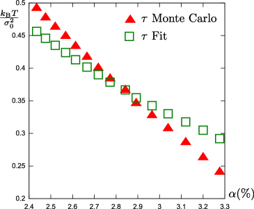
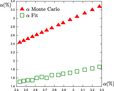
Refer to caption
(a) Tension τ𝜏\tau.
Refer to caption
(b) Excess area.
Figure 7.21: At left, we show with the red triangles the measured values of τ𝜏\tau in units of kBT/σ02subscript𝑘B𝑇superscriptsubscript𝜎02k_{\mathrm{B}}T/\sigma_{0}^{2}. We have fitted eq.(7.24) to the red triangles by adjusting ΛΛ\Lambda. The best result, obtained for Λ=1.03σ01Λ1.03superscriptsubscript𝜎01\Lambda=1.03\,\sigma_{0}^{-1}, is shown with green squares. At right, we applied this value of ΛΛ\Lambda to eq.(7.25) and obtained the predicted excess area (green squares), which are clearly incompatible with the measured excess area (red triangles).

In chapter 2, we have also predicted the dependence of the excess area on the tension σ𝜎\sigma:

α=kBT8πκln(σrσ).𝛼subscript𝑘B𝑇8𝜋𝜅subscript𝜎𝑟𝜎\alpha=\frac{k_{\mathrm{B}}T}{8\pi\kappa}\ln\left(\frac{\sigma_{r}}{\sigma}\right)\,. (7.25)

Both eqs.(7.24) and (7.25) should be valid under the same conditions. Accordingly, we decided to make a self-consistency test by plotting the predicted values of the excess area obtained through eq.(7.25), with the ΛΛ\Lambda obtained above. We observe that the predicted values for the excess area are consistently smaller than the values measured during the simulation.

Up to now, we have not a clear explanation for these results. Two hypothesis deserve further attention:

  • our membrane is not exactly very tense, since it is very easy to stretch the bonds. Indeed, stretching a bond to its maximum costs only 0.25kBTsimilar-toabsent0.25subscript𝑘B𝑇\sim 0.25k_{\mathrm{B}}T for βσ02s=1𝛽superscriptsubscript𝜎02𝑠1\beta\,\sigma_{0}^{2}\,s=1. It is thus possible that the simulated membrane is not under the hypothesis of our theory. We could thus imagine further tests with a higher s𝑠s, but in this case, as discussed earlier, the membrane would loose its liquidity.

  • the projected area of the membrane could be bigger, which would explain why the measured excess area is consistently bigger than the predicted. When we proposed the equilibration criteria in section 7.3.1, we studied the average shape of the membrane, as shown in Fig. 7.12. We have not however excluded the possibility of a rotating deformed shape: in this case, we would still have an average shape nearly flat, but the membrane would actually fluctuate around this deformed shape, with a projected area bigger than if it fluctuated effectively around a plane. To verify that, we should perform a rotation to align the configurations before evaluating the average shape by aligning the direction of the maximum height at each step, for instance. This would however not explain the poor fit shown in Fig. 7.21(a).

7.6 Extraction of tubes

In parallel with the studies on the membrane tension, we have explored the possibility of extracting tubes from our simplified membrane. To pull a tube, we have applied a harmonic potential

Vtube=ktube(hh0)22,subscript𝑉tubesubscript𝑘tubesuperscriptsubscript022V_{\mathrm{tube}}=k_{\mathrm{tube}}\,\frac{(h-h_{0})^{2}}{2}\,, (7.26)

to a central bead whose height is denoted by hh. The preferred height of the tube is defined by the choice of h0subscript0h_{0}. As in the case of the frame’s force, we could obtain the force applied to pull the tube, as well as its fluctuation. The first results for the same parameters of the last section, with Rf=33.04σ0subscript𝑅𝑓33.04subscript𝜎0R_{f}=33.04\,\sigma_{0}, are shown in Fig. 7.22.

Refer to caption
(a) h0=10σ0subscript010subscript𝜎0h_{0}=10\,\sigma_{0}.
Refer to caption
(b) h0=15σ0subscript015subscript𝜎0h_{0}=15\,\sigma_{0}.
Figure 7.22: Tube pulled from a membrane for two different values of h0subscript0h_{0}. At right, remark that the angle between the triangles is very important in the protruded region. The vertical and horizontal scales are different.

Looking at these images, we remark a first problem: the angle between the triangles is very large. This phenomenon is still more marked for a bigger tubes (see Fig. 7.23(a)), where the protuberance becomes almost flat. The problem comes from the discretization of the curvature energy:

Eκdiscret=kα,β(1𝒏α𝒏β),superscriptsubscript𝐸𝜅discret𝑘subscript𝛼𝛽1subscript𝒏𝛼subscript𝒏𝛽E_{\kappa}^{\mathrm{discret}}=k\sum_{\langle\alpha,\beta\rangle}(1-\bm{n}_{\alpha}\cdot\bm{n}_{\beta})\,, (7.27)

where α𝛼\alpha and β𝛽\beta are adjacent triangles. As discussed before, this discretization is valid only for 𝒏α𝒏βsubscript𝒏𝛼subscript𝒏𝛽\bm{n}_{\alpha}\approx\bm{n}_{\beta}, since large deformations bear an unphysical finite cost. We proposed thus an alternative discretization

Eκdiscret=kα,β(1𝒏α𝒏β)e0.8(1+𝒏α𝒏β).superscriptsubscriptsuperscript𝐸𝜅discret𝑘subscript𝛼𝛽1subscript𝒏𝛼subscript𝒏𝛽superscript𝑒0.81subscript𝒏𝛼subscript𝒏𝛽{E^{\prime}}_{\kappa}^{\mathrm{discret}}=k\sum_{\langle\alpha,\beta\rangle}(1-\bm{n}_{\alpha}\cdot\bm{n}_{\beta})\,e^{\frac{0.8}{(1+\bm{n}_{\alpha}\cdot\bm{n}_{\beta})}}\,. (7.28)

With this discretization, the energy cost is roughly the same as before for 𝒏α𝒏βsubscript𝒏𝛼subscript𝒏𝛽\bm{n}_{\alpha}\approx\bm{n}_{\beta}, but it increases exponentially as 𝒏αsubscript𝒏𝛼\bm{n}_{\alpha} approaches 𝒏βsubscript𝒏𝛽-\bm{n}_{\beta}. The resulting tube, with the same parameters as in Fig. 7.23(a), has a more normal appearance (see Fig. 7.23(b)).

Refer to caption
(a) h0=20σ0subscript020subscript𝜎0h_{0}=20\,\sigma_{0} with eq.(7.27).
Refer to caption
(b) h0=20σ0subscript020subscript𝜎0h_{0}=20\,\sigma_{0} with eq.(7.28).
Figure 7.23: Tubes pulled from membranes with the same parameters as before, but with different discretizations for the curvature energy. The vertical and horizontal scales are different. At left, we see an almost flat protuberance, while at right we see a normal tube.

Due to time constraints, we have not examined the dependence of the force needed to extract a tube as a function of its radius. It would also be interesting to measure the tube’s radius: together with the measure of the force, one could thus deduce the tension σ𝜎\sigma and the bending rigidity κ𝜅\kappa.

7.7 Perspectives and discussion

As mentioned at the beginning of this chapter, we presented here only preliminary results and many issues need further attention, such as:

  1. 1.

    verify more carefully if the average shape of the membrane is indeed planar.

  2. 2.

    study the dependence of ΔτΔ𝜏\Delta\tau on σ𝜎\sigma.

  3. 3.

    in section 2.4.1 of chapter 2, we predicted that for a membrane under no external force, i. e., with τ=0𝜏0\tau=0, the natural excess area was given by

    αeqln(8πβκ)8πβκ,similar-to-or-equalssubscript𝛼eq8𝜋𝛽𝜅8𝜋𝛽𝜅\alpha_{\mathrm{eq}}\simeq\frac{\ln(8\pi\beta\kappa)}{8\pi\beta\kappa}\,, (7.29)

    which depends only on the membrane bending rigidity and temperature. If however one forgets the difference between τ𝜏\tau and σ𝜎\sigma, αeqsubscript𝛼eq\alpha_{\mathrm{eq}} should also depend logarithmically on the size of the membrane (see eq.(2.77)). Numerically, we could thus adjust the frame’s radius Rfsubscript𝑅𝑓R_{f} for different membrane sizes in order to have τ=0delimited-⟨⟩𝜏0\langle\tau\rangle=0 and measure the excess area in each case.

  4. 4.

    study better the extraction of tubes and the effects of the alternative discretization of the curvature energy proposed by us.

  5. 5.

    perform a systematic study on the time needed for a system to equilibrate as a function of its size and parameters.

At last, even if using a network to simulate a membrane presents many advantages, it presents a severe drawback: in order to assure liquidity, the bonds must be very easily stretched. To make the bonds stiffer without affecting the membrane liquidity, one possible solution would be to pass to a macrocanonical ensemble of effective particles: the network would have thus a non-fixed number of beads. A new particle could be introduced in the middle of a very stretched triangle, which would restore the liquidity for the case of high tension. Conversely, beads should also be deleted from the network. In practice, this is very difficult to implement already from a data structure point of view and the results are not sure.

7.8 In a nutshell

In this chapter we presented some preliminary results of a numerical experiment consisting in a piece of weakly fluctuating membrane attached to a circular frame. Numerically, it was represented by a triangular network whose connectivity evolved to simulate liquidity. At each vertex of the network, we placed effective particles that could interact with their first neighbors. The bending rigidity was mimicked by an interaction between adjacent triangles and the particles in the network’s edge were submitted to a harmonic potential in order to force the circular frame. We used a Monte Carlo method to obtain a large sample of equilibrium configurations, from which we could evaluate averages of the mechanical tension, excess area and fluctuation spectrum. Our first results seems to show that the network behaves similarly to a membrane, but we could not quantitatively verify our predictions concerning the membrane tension. Many questions in this chapter were left untackled due to time constraints.

Conclusion

Lipid membranes are very particular materials: despite being almost unstretchable microscopically, in mesoscopic scale they can be easily stretched through the flattening of thermal fluctuations. Indeed, lipid membranes are highly fluctuating and present thus an excess area relative to its optically resolvable area.

In the beginning of this work, we have seen that the term surface tension designates several quantities in the context of lipid membranes. First, there is the tension τ𝜏\tau needed to increase the projected area, or equivalently, to reduce the excess area. Secondly, there is σ𝜎\sigma, the Lagrange-multiplier introduced theoretically to impose a fixed microscopical area to the membrane. Finally, there is the macroscopic counterpart of σ𝜎\sigma, r𝑟r, related to the spectrum of fluctuation.

Experimentally, r𝑟r can be obtained directly from the fluctuation spectrum and τ𝜏\tau can be measured through the Laplace pressure, for instance. On the other hand, the theoretical predictions usually involve σ𝜎\sigma, which is not directly measurable. To interpret experimental data, the equality between these quantities is often taken for granted. Our main goal throughout this work was to determine under which conditions these suppositions are justifiable, specially the equality between τ𝜏\tau and σ𝜎\sigma.

Firstly, we have treated the simplest case of a planar membrane. In the literature, we find some former calculations relating τ𝜏\tau to σ𝜎\sigma and r𝑟r. There was, however, no consensus: different results were found, depending on how the calculation was made and on the precise definition of τ𝜏\tau. Indeed, the method involved deriving the free-energy with respect to the projected area of the membrane, which we have shown here to be very tricky. To work around this problem, we have chosen to use a more recent tool: the projected stress tensor, a tensor that relates the force exchanged through an infinitesimal cut on the membrane to the projection of this cut on the projected plane. The definition of the mechanical tension τ𝜏\tau is thus straightforward: it is simply given by the average of the projected stress tensor. As supplemental advantage, the projected stress tensor can be relatively easily derived for other geometries, such as spherical and cylindrical, which we have treated in this dissertation.

After evaluating the average of the projected stress tensor, we have obtained an exact relation between τ𝜏\tau and σ𝜎\sigma for weakly fluctuating planar membranes. In a general way, we have τσσ0similar-to-or-equals𝜏𝜎subscript𝜎0\tau\simeq\sigma-\sigma_{0}, which is the most important result of this dissertation. The constant σ0subscript𝜎0\sigma_{0} depends on the temperature and on the frequency cutoff ΛΛ\Lambda, i. e., the highest wave-vector allowed. At room temperature and considering Λ=1/(5nm)Λ15nm\Lambda=1/(5\,\mathrm{nm}), we find σ05×106N/msubscript𝜎05superscript106Nm\sigma_{0}\approx 5\times 10^{-6}\,\mathrm{N/m}. Accordingly, the assumption στ𝜎𝜏\sigma\approx\tau is justifiable only for high tensions. Otherwise, one must consider the corrected relation to interpret correctly experimental data. Indeed, some experiments on the adhesion of vesicles seems to agree with our predictions.

In laboratory, planar membranes are very difficult to manipulate. Vesicles are more commonly used, specially the giant vesicles that can be easily manipulated with a micropipette. These vesicles can be poked, i. e., free to exchange inner material with the suspension medium, or closed, i. e., with a fixed volume. We examined thus how the volume constraint and the geometry affected the above mentioned relation for quasi-spherical vesicles. For both poked and closed vesicles, we conclude that the relation obtained in the planar case is a very good approximation. Interestingly, we predict that the internal pressure of a spherical vesicle can be smaller than the outer, which is impossible in liquid drops.

Another popularly geometry found in membrane experiments is the cylinder. Indeed, nanotubes are extracted from a piece of membrane, typically a vesicle, by applying a point force with an optical tweezer or with a magnetic field. Using a simplified mean-field calculations and supposing στ𝜎𝜏\sigma\approx\tau, the bending rigidity is usually obtained from the curve force versus tension. Recently, however, theoretical calculations have predicted that the shape fluctuations for this geometry are very strong. We expect hence that these fluctuations may affect the interpretation of force measurements. In this work, we have found that these fluctuation do affect indeed the value of the mean-field force. Curiously, the effect has never been observed, since the assumption στ𝜎𝜏\sigma\approx\tau seems to coincidently make up for the thermal fluctuations.

Aside from the evaluation of tensions and forces, we have also evaluated for the first time the standard deviation of these quantities due to thermal fluctuations. As in tubular geometry the shape fluctuations are important, we would like to verify if the fluctuation of the force needed to extract a membrane tube could be used to characterize a membrane. Our results show that the force fluctuation depends on the temperature and that it is very sensitive to the values of ΛΛ\Lambda, whereas it does almost not depend on the bending rigidity nor on the tension. It should thus be of little usefulness to characterize mechanically a membrane. On the other hand, it is possibly interesting to study the activity of active proteins embedded in the membrane, which has an effect similar to changing temperature.

Finally, while we have characterized rather well the relation between τ𝜏\tau and σ𝜎\sigma, we leave almost untackled the question of how r𝑟r relates to the other tensions: we have just questioned a former prediction stating that r=τ𝑟𝜏r=\tau and observed a non-trivial behavior of r𝑟r in two numerical experiments proposed by us. The question is however very important and needs further attention, since r𝑟r is a popular non-invasive method used to accede to the tension of a membrane.

Appendix A Alternative derivation of the projected stress tensor

We re-derive here eqs.(1.58)–(1.60) directly from eq.(1.50). We consider a local tangent frame (X,Y,Z)𝑋𝑌𝑍(X,Y,Z) attached to the membrane, with the first two axes parallel to the principal curvature directions and the third one parallel to the membrane normal, as shown in Fig. 1.38(a). In this principal tangent frame, as introduced in section 1.5.1, the force exchanged through a cut of length d𝑑superscriptd\ell^{\prime} is given by

dϕ=𝚺~𝝂d,𝑑bold-italic-ϕ~𝚺𝝂𝑑superscriptd\bm{\phi}=\tilde{\bm{\Sigma}}\cdot\bm{\nu}\,d\ell^{\prime}\,, (A.1)

where 𝝂𝝂\bm{\nu} is the normal to the cut within the tangent plane and𝚺~~𝚺\tilde{\bm{\Sigma}} is given by eq.(1.50).

Now, consider the fixed reference plane ΠΠ\Pi introduced on section 1.5.2. The projected stress tensor 𝚺𝚺\bm{\Sigma} is defined by

dϕ=𝚺𝒎d,𝑑bold-italic-ϕ𝚺𝒎𝑑d\bm{\phi}=\bm{\Sigma}\cdot\bm{m}\,d\ell\,, (A.2)

where d𝑑d\ell is the length of the cut’s projection onto ΠΠ\Pi and 𝒎𝒎\bm{m} the normal to the cut’s projection within ΠΠ\Pi (see Fig. 1.39). We aim to obtain 𝚺𝚺\bm{\Sigma} by comparing eq.(A.1) and eq.(A.2) when the membrane normal exhibits only small deviations with respect to the normal to ΠΠ\Pi.

We consider an orthonormal basis (x,y,z)𝑥𝑦𝑧(x,y,z) with 𝒆xsubscript𝒆𝑥\bm{e}_{x} and 𝒆ysubscript𝒆𝑦\bm{e}_{y} belonging to ΠΠ\Pi. We choose 𝒎=𝒆x𝒎subscript𝒆𝑥\bm{m}=\bm{e}_{x}, the cut’s projection being parallel to 𝒆ysubscript𝒆𝑦\bm{e}_{y}. Locally, the membrane shape may be approximated by a quadratic form:

z=h(x,y)h0+ax+by+12αx2+βxy+12γy2,𝑧𝑥𝑦similar-to-or-equalssubscript0𝑎𝑥𝑏𝑦12𝛼superscript𝑥2𝛽𝑥𝑦12𝛾superscript𝑦2z=h(x,y)\simeq h_{0}+a\,x+b\,y+\frac{1}{2}\,\alpha\,x^{2}+\beta\,xy+\frac{1}{2}\,\gamma\,y^{2}\,, (A.3)

with (a,b,α,β,γ)(hx,hy,hxx,hxy,hyy)=𝒪(ϵ)𝑎𝑏𝛼𝛽𝛾subscript𝑥subscript𝑦subscript𝑥𝑥subscript𝑥𝑦subscript𝑦𝑦𝒪italic-ϵ(a,b,\alpha,\beta,\gamma)\equiv(h_{x},h_{y},h_{xx},h_{xy},h_{yy})=\mathcal{O}(\epsilon) and ϵ1much-less-thanitalic-ϵ1\epsilon\ll 1. We shall apply three successive frame rotations in order to bring the fixed frame (x,y,z)𝑥𝑦𝑧(x,y,z) to the tangent principal frame (X,Y,Z)𝑋𝑌𝑍(X,Y,Z).

First, we make a rotation about 𝒆xsubscript𝒆𝑥\bm{e}_{x} of angle θ1=bsubscript𝜃1𝑏\theta_{1}=b, plus a vertical translation. The new coordinates, indicated by a prime, are related to the old ones by

x𝑥\displaystyle x =\displaystyle= x,superscript𝑥\displaystyle x^{\prime}\,, (A.4)
y𝑦\displaystyle y =\displaystyle= (1b22)ybz+𝒪(ϵ3),1superscript𝑏22superscript𝑦𝑏superscript𝑧𝒪superscriptitalic-ϵ3\displaystyle\left(1-\frac{b^{2}}{2}\right)y^{\prime}-b\,z^{\prime}+\mathcal{O}(\epsilon^{3})\,, (A.5)
z𝑧\displaystyle z =\displaystyle= h0+by+(1b22)z+𝒪(ϵ3).subscript0𝑏superscript𝑦1superscript𝑏22superscript𝑧𝒪superscriptitalic-ϵ3\displaystyle h_{0}+b\,y^{\prime}+\left(1-\frac{b^{2}}{2}\right)z^{\prime}+\mathcal{O}(\epsilon^{3})\,. (A.6)

Note that 𝒆ysuperscriptsubscript𝒆𝑦\bm{e}_{y}^{\prime} is thus parallel to the actual cut within the membrane. We perform a second rotation, about the new axis 𝒆ysuperscriptsubscript𝒆𝑦\bm{e}_{y}^{\prime} of angle θ2=asubscript𝜃2𝑎\theta_{2}=a in order to make the new plane (x′′,y′′)superscript𝑥′′superscript𝑦′′(x^{\prime\prime},y^{\prime\prime}) coincide with the tangent plane:

xsuperscript𝑥\displaystyle x^{\prime} =\displaystyle= (1a22)x′′az′′+𝒪(ϵ3),1superscript𝑎22superscript𝑥′′𝑎superscript𝑧′′𝒪superscriptitalic-ϵ3\displaystyle\left(1-\frac{a^{2}}{2}\right)x^{\prime\prime}-a\,z^{\prime\prime}+\mathcal{O}(\epsilon^{3})\,, (A.7)
ysuperscript𝑦\displaystyle y^{\prime} =\displaystyle= y′′,superscript𝑦′′\displaystyle y^{\prime\prime}\,, (A.8)
zsuperscript𝑧\displaystyle z^{\prime} =\displaystyle= ax′′+(1a22)z′′+𝒪(ϵ3).𝑎superscript𝑥′′1superscript𝑎22superscript𝑧′′𝒪superscriptitalic-ϵ3\displaystyle a\,x^{\prime\prime}+\left(1-\frac{a^{2}}{2}\right)z^{\prime\prime}+\mathcal{O}(\epsilon^{3})\,. (A.9)

Note that 𝒆y′′𝒆ysuperscriptsubscript𝒆𝑦′′superscriptsubscript𝒆𝑦\bm{e}_{y}^{\prime\prime}\equiv\bm{e}_{y}^{\prime} is still parallel to the actual cut, while 𝒆x′′superscriptsubscript𝒆𝑥′′\bm{e}_{x}^{\prime\prime} is now the normal to the cut within the tangent plane. In other words 𝒆x′′=𝝂superscriptsubscript𝒆𝑥′′𝝂\bm{e}_{x}^{\prime\prime}=\bm{\nu}.

In the (x′′,y′′,z′′)superscript𝑥′′superscript𝑦′′superscript𝑧′′(x^{\prime\prime},y^{\prime\prime},z^{\prime\prime}) coordinate system, the membrane shape is given simply by

z′′=12αx′′2+βx′′y′′+12γy′′2+𝒪(ϵ3).superscript𝑧′′12𝛼superscript𝑥′′2𝛽superscript𝑥′′superscript𝑦′′12𝛾superscript𝑦′′2𝒪superscriptitalic-ϵ3z^{\prime\prime}=\frac{1}{2}\,\alpha\,x^{\prime\prime 2}+\beta\,x^{\prime\prime}y^{\prime\prime}+\frac{1}{2}\,\gamma\,y^{\prime\prime 2}+\mathcal{O}(\epsilon^{3})\,. (A.10)

Finally, we arrive to the principal tangent frame (X,Y,Z)𝑋𝑌𝑍(X,Y,Z) by making a rotation about 𝒆z′′subscript𝒆superscript𝑧′′\bm{e}_{z^{\prime\prime}} in order to diagonalize the quadratic form. Indeed, if we set

x′′superscript𝑥′′\displaystyle x^{\prime\prime} =\displaystyle= XcosθYsinθ,𝑋𝜃𝑌𝜃\displaystyle X\cos\theta-Y\sin\theta\,, (A.11)
y′′superscript𝑦′′\displaystyle y^{\prime\prime} =\displaystyle= Xsinθ+Ycosθ,𝑋𝜃𝑌𝜃\displaystyle X\sin\theta+Y\cos\theta\,, (A.12)
z′′superscript𝑧′′\displaystyle z^{\prime\prime} =\displaystyle= Z,𝑍\displaystyle Z\,, (A.13)

where θ𝜃\theta is the solution of

2βcos2θ=(αγ)sin2θ,2𝛽2𝜃𝛼𝛾2𝜃2\beta\,\cos 2\theta=(\alpha-\gamma)\sin 2\theta\,, (A.14)

the cross term vanishes, leaving Z=12CXX2+12CYY2𝑍12subscript𝐶𝑋superscript𝑋212subscript𝐶𝑌superscript𝑌2Z=\frac{1}{2}\,C_{X}X^{2}+\frac{1}{2}\,C_{Y}Y^{2}, where CX=αcos2θ+γsin2θ+βsin2θ+𝒪(ϵ3)subscript𝐶𝑋𝛼superscript2𝜃𝛾superscript2𝜃𝛽2𝜃𝒪superscriptitalic-ϵ3C_{X}=\alpha\cos^{2}\theta+\gamma\sin^{2}\theta+\beta\sin 2\theta+\mathcal{O}(\epsilon^{3}) and CY=γcos2θ+αsin2θβsin2θ+𝒪(ϵ3)subscript𝐶𝑌𝛾superscript2𝜃𝛼superscript2𝜃𝛽2𝜃𝒪superscriptitalic-ϵ3C_{Y}=\gamma\cos^{2}\theta+\alpha\sin^{2}\theta-\beta\sin 2\theta+\mathcal{O}(\epsilon^{3}) are the principal curvatures.

Comparing eqs.(A.1) and (A.2) while using 𝒎=𝒆x𝒎subscript𝒆𝑥\bm{m}=\bm{e}_{x}, 𝝂=𝒆x′′𝝂subscript𝒆superscript𝑥′′\bm{\nu}=\bm{e}_{x^{\prime\prime}} and d=d(1+b2/2)+𝒪(ϵ3)𝑑superscript𝑑1superscript𝑏22𝒪superscriptitalic-ϵ3d\ell^{\prime}=d\ell(1+b^{2}/2)+\mathcal{O}(\epsilon^{3}), yields

Σxx=(1+b22)𝒆x𝚺~𝒆x′′+𝒪(ϵ3),subscriptΣ𝑥𝑥1superscript𝑏22subscript𝒆𝑥~𝚺subscript𝒆superscript𝑥′′𝒪superscriptitalic-ϵ3\displaystyle\Sigma_{xx}=\left(1+\frac{b^{2}}{2}\right)\bm{e}_{x}\cdot\tilde{\bm{\Sigma}}\cdot\bm{e}_{x^{\prime\prime}}+\mathcal{O}(\epsilon^{3})\,, (A.15)
Σyx=(1+b22)𝒆y𝚺~𝒆x′′+𝒪(ϵ3),subscriptΣ𝑦𝑥1superscript𝑏22subscript𝒆𝑦~𝚺subscript𝒆superscript𝑥′′𝒪superscriptitalic-ϵ3\displaystyle\Sigma_{yx}=\left(1+\frac{b^{2}}{2}\right)\bm{e}_{y}\cdot\tilde{\bm{\Sigma}}\cdot\bm{e}_{x^{\prime\prime}}+\mathcal{O}(\epsilon^{3})\,, (A.16)
Σzx=(1+b22)𝒆z𝚺~𝒆x′′+𝒪(ϵ3).subscriptΣ𝑧𝑥1superscript𝑏22subscript𝒆𝑧~𝚺subscript𝒆superscript𝑥′′𝒪superscriptitalic-ϵ3\displaystyle\Sigma_{zx}=\left(1+\frac{b^{2}}{2}\right)\bm{e}_{z}\cdot\tilde{\bm{\Sigma}}\cdot\bm{e}_{x^{\prime\prime}}+\mathcal{O}(\epsilon^{3})\,. (A.17)

Calculating 𝚺~𝒆x′′~𝚺subscript𝒆superscript𝑥′′\tilde{\bm{\Sigma}}\cdot\bm{e}_{x^{\prime\prime}} from eq.(1.50), we obtain

𝚺~𝒆x′′~𝚺subscript𝒆superscript𝑥′′\displaystyle\tilde{\bm{\Sigma}}\cdot\bm{e}_{x^{\prime\prime}} =\displaystyle= cosθ(σ+κ2CY2κ2CX2)𝒆X𝜃𝜎𝜅2superscriptsubscript𝐶𝑌2𝜅2superscriptsubscript𝐶𝑋2subscript𝒆𝑋\displaystyle\cos\theta\left(\sigma+\frac{\kappa}{2}\,C_{Y}^{2}-\frac{\kappa}{2}\,C_{X}^{2}\right)\bm{e}_{X} (A.18)
\displaystyle- sinθ(σ+κ2CX2κ2CY2)𝒆Y𝜃𝜎𝜅2superscriptsubscript𝐶𝑋2𝜅2superscriptsubscript𝐶𝑌2subscript𝒆𝑌\displaystyle\sin\theta\left(\sigma+\frac{\kappa}{2}\,C_{X}^{2}-\frac{\kappa}{2}\,C_{Y}^{2}\right)\bm{e}_{Y}
\displaystyle- κCx′′𝒆Z,𝜅𝐶superscript𝑥′′subscript𝒆𝑍\displaystyle\kappa\,\frac{\partial C}{\partial x^{\prime\prime}}\bm{e}_{Z}\,,

with C=2h+𝒪(ϵ2)𝐶superscript2𝒪superscriptitalic-ϵ2C=\nabla^{2}h+\mathcal{O}(\epsilon^{2}). We have taken advantage that the terms 𝒆Zproportional-toabsentsubscript𝒆𝑍\propto\bm{e}_{Z} in eq.(1.50) are equal κ𝒆ZCtensor-product𝜅subscript𝒆𝑍bold-∇𝐶-\kappa\,\bm{e}_{Z}\otimes\bm{\nabla}C. Going to the (x′′,y′′,z′′)superscript𝑥′′superscript𝑦′′superscript𝑧′′(x^{\prime\prime},y^{\prime\prime},z^{\prime\prime}) basis and using eq.(A.14), we have simply

𝚺~𝒆x′′~𝚺subscript𝒆superscript𝑥′′\displaystyle\tilde{\bm{\Sigma}}\cdot\bm{e}_{x^{\prime\prime}} =\displaystyle= (σ+κ2γ2κ2α2)𝒆x′′𝜎𝜅2superscript𝛾2𝜅2superscript𝛼2subscript𝒆superscript𝑥′′\displaystyle\left(\sigma+\frac{\kappa}{2}\,\gamma^{2}-\frac{\kappa}{2}\,\alpha^{2}\right)\bm{e}_{x^{\prime\prime}} (A.19)
\displaystyle- κ2β(α+γ)𝒆y′′κCx′′𝒆z′′+𝒪(ϵ3).𝜅2𝛽𝛼𝛾subscript𝒆superscript𝑦′′𝜅𝐶superscript𝑥′′subscript𝒆superscript𝑧′′𝒪superscriptitalic-ϵ3\displaystyle\frac{\kappa}{2}\,\beta\left(\alpha+\gamma\right)\bm{e}_{y^{\prime\prime}}-\kappa\,\frac{\partial C}{\partial x^{\prime\prime}}\,\bm{e}_{z^{\prime\prime}}+\mathcal{O}(\epsilon^{3})\,.\qquad

Since C=𝒪(ϵ)𝐶𝒪italic-ϵC=\mathcal{O}(\epsilon), we can replace /x′′superscript𝑥′′\partial/\partial x^{\prime\prime} by /x𝑥\partial/\partial x, since the difference between the latter is of order ϵ2superscriptitalic-ϵ2\epsilon^{2}. Using now directly eqs.(A.15)–(A.17), with 𝒆x′′𝒆x=(1a2/2)+𝒪(ϵ3)subscript𝒆superscript𝑥′′subscript𝒆𝑥1superscript𝑎22𝒪superscriptitalic-ϵ3\bm{e}_{x^{\prime\prime}}\cdot\bm{e}_{x}=(1-a^{2}/2)+\mathcal{O}(\epsilon^{3}), 𝒆y′′𝒆x=0subscript𝒆superscript𝑦′′subscript𝒆𝑥0\bm{e}_{y^{\prime\prime}}\cdot\bm{e}_{x}=0, 𝒆z′′𝒆x=a+𝒪(ϵ3)subscript𝒆superscript𝑧′′subscript𝒆𝑥𝑎𝒪superscriptitalic-ϵ3\bm{e}_{z^{\prime\prime}}\cdot\bm{e}_{x}=-a+\mathcal{O}(\epsilon^{3}), etc., yields

ΣxxsubscriptΣ𝑥𝑥\displaystyle\Sigma_{xx} =\displaystyle= σ+σ2(b2a2)+κ2(γ2α2)𝜎𝜎2superscript𝑏2superscript𝑎2𝜅2superscript𝛾2superscript𝛼2\displaystyle\sigma+\frac{\sigma}{2}\left(b^{2}-a^{2}\right)+\frac{\kappa}{2}\left(\gamma^{2}-\alpha^{2}\right) (A.20)
+κaxC+𝒪(ϵ3),𝜅𝑎subscript𝑥𝐶𝒪superscriptitalic-ϵ3\displaystyle+\kappa\,a\,\partial_{x}C+\mathcal{O}(\epsilon^{3})\,,
ΣyxsubscriptΣ𝑦𝑥\displaystyle\Sigma_{yx} =\displaystyle= σabκβ(α+γ)+κbxC+𝒪(ϵ3),𝜎𝑎𝑏𝜅𝛽𝛼𝛾𝜅𝑏subscript𝑥𝐶𝒪superscriptitalic-ϵ3\displaystyle-\sigma\,ab-\kappa\,\beta\left(\alpha+\gamma\right)+\kappa\,b\,\partial_{x}C+\mathcal{O}(\epsilon^{3})\,,\qquad (A.21)
ΣzxsubscriptΣ𝑧𝑥\displaystyle\Sigma_{zx} =\displaystyle= σaκxC+𝒪(ϵ3),𝜎𝑎𝜅subscript𝑥𝐶𝒪superscriptitalic-ϵ3\displaystyle\sigma a-\kappa\,\partial_{x}C+\mathcal{O}(\epsilon^{3})\,, (A.22)

which coincide with eqs.(1.58)–(1.60).

Appendix B Projected stress tensor for a 111-d filament

The derivation of the projected stress tensor for a 111-d filament follows the same reasoning presented in section 1.5.2. The force exchanged through a cut is given by

𝒇=𝚺1D𝒎=(Σx1D𝒆x+Σz1D𝒆z)mx,𝒇superscript𝚺1D𝒎subscriptsuperscriptΣ1D𝑥subscript𝒆𝑥subscriptsuperscriptΣ1D𝑧subscript𝒆𝑧subscript𝑚𝑥\bm{f}=\bm{\Sigma}^{\mathrm{1D}}\cdot\bm{m}=\left(\Sigma^{\mathrm{1D}}_{x}\,\bm{e}_{x}+\Sigma^{\mathrm{1D}}_{z}\,\bm{e}_{z}\right)m_{x}\,, (B.1)

where 𝒎=mx𝒆𝒙=±𝒆x𝒎subscript𝑚𝑥subscript𝒆𝒙plus-or-minussubscript𝒆𝑥\bm{m}=m_{x}\,\bm{e_{x}}=\pm\,\bm{e}_{x}, depending on the orientation of the projected cut. Note that the stress tensor now has just two components. For a general filament whose energy is given by

=Lpf(hx,hxx)𝑑x,subscriptsubscript𝐿𝑝𝑓subscript𝑥subscript𝑥𝑥differential-d𝑥\mathcal{H}=\int_{L_{p}}f(h_{x},h_{xx})\,dx\,, (B.2)

an arbitrary small displacement δ𝒂=δax𝒆x+δaz𝒆z𝛿𝒂𝛿subscript𝑎𝑥subscript𝒆𝑥𝛿subscript𝑎𝑧subscript𝒆𝑧\delta\bm{a}=\delta a_{x}\,\bm{e}_{x}+\delta a_{z}\,\bm{e}_{z} of the membrane, at equilibrium, leads to the energy variation

δ=[fδax+(fhxxfhxx)δufhxxδux]mx|δLp,𝛿evaluated-atdelimited-[]𝑓𝛿subscript𝑎𝑥𝑓subscript𝑥subscript𝑥𝑓subscript𝑥𝑥𝛿𝑢𝑓subscript𝑥𝑥𝛿subscript𝑢𝑥subscript𝑚𝑥𝛿subscript𝐿𝑝\delta\mathcal{H}=\left.\left[f\,\delta a_{x}+\left(\frac{\partial f}{\partial h_{x}}-\partial_{x}\frac{\partial f}{\partial h_{xx}}\right)\delta u-\frac{\partial f}{\partial h_{xx}}\,\delta u_{x}\right]m_{x}\right|_{\delta L_{p}}\,, (B.3)

where δLp𝛿subscript𝐿𝑝\delta L_{p} indicates a sum over the two edges of the filament. Keeping the tangent to the filament at the edges unchanged so that torques perform no work, we have

δu=δazδazhx,𝛿𝑢𝛿subscript𝑎𝑧𝛿subscript𝑎𝑧subscript𝑥\delta u=\delta a_{z}-\delta a_{z}\,h_{x}\,, (B.4)

and

δux=δaxhxx.𝛿subscript𝑢𝑥𝛿subscript𝑎𝑥subscript𝑥𝑥\delta u_{x}=-\,\delta a_{x}\,h_{xx}\,. (B.5)

Finally, comparing the work of the force 𝒇𝒇\bm{f} given in eq.(B.1) and the work given in eq.(B.3), using eq.(B.4) and eq.(B.5), we obtain

Σx1DsubscriptsuperscriptΣ1D𝑥\displaystyle\Sigma^{\mathrm{1D}}_{x} =\displaystyle= ffhxhxfhxxhxx+x(fhxx)hx,𝑓𝑓subscript𝑥subscript𝑥𝑓subscript𝑥𝑥subscript𝑥𝑥subscript𝑥𝑓subscript𝑥𝑥subscript𝑥\displaystyle f-\frac{\partial f}{\partial h_{x}}h_{x}-\frac{\partial f}{\partial h_{xx}}h_{xx}+\partial_{x}\left(\frac{\partial f}{\partial h_{xx}}\right)h_{x}\,,
Σz1DsubscriptsuperscriptΣ1D𝑧\displaystyle\Sigma^{\mathrm{1D}}_{z} =\displaystyle= fhxx(fhxx).𝑓subscript𝑥subscript𝑥𝑓subscript𝑥𝑥\displaystyle\frac{\partial f}{\partial h_{x}}-\partial_{x}\left(\frac{\partial f}{\partial h_{xx}}\right)\,. (B.6)

For 1Dsubscript1D\mathcal{H}_{\mathrm{1D}} (eq.(2.44), we have

Σx1DsubscriptsuperscriptΣ1D𝑥\displaystyle\Sigma^{\mathrm{1D}}_{x} =\displaystyle= σσ2hx2κ2hxx2+κhxxxhx,𝜎𝜎2superscriptsubscript𝑥2𝜅2superscriptsubscript𝑥𝑥2𝜅subscript𝑥𝑥𝑥subscript𝑥\displaystyle\sigma-\frac{\sigma}{2}h_{x}^{2}-\frac{\kappa}{2}h_{xx}^{2}+\kappa\,h_{xxx}h_{x}\,,
Σz1DsubscriptsuperscriptΣ1D𝑧\displaystyle\Sigma^{\mathrm{1D}}_{z} =\displaystyle= σhxκhxxx.𝜎subscript𝑥𝜅subscript𝑥𝑥𝑥\displaystyle\sigma\,h_{x}-\kappa\,h_{xxx}\,. (B.7)

Appendix C Estimative of 𝑾𝑨𝐭𝐡𝐞𝐨superscriptsubscript𝑾𝑨𝐭𝐡𝐞𝐨\bm{W_{A}^{\mathrm{theo}}}

In this section we explain in details the theoretical estimative of the adhesion energy per unit area WAtheosuperscriptsubscript𝑊𝐴theoW_{A}^{\mathrm{theo}} proposed by Rädler et al. [84]. They took into account two attractive interactions, coming from the van der Waals interactions and gravity, and a repulsive interaction with entropic origins, due to the restrictions imposed on the membrane fluctuation. They considered the screened van der Waals potential given by

VvdW=AH12π[1s21(s+a)2](2sλDe2sλD),subscript𝑉vdWsubscript𝐴𝐻12𝜋delimited-[]1superscript𝑠21superscript𝑠𝑎22𝑠subscript𝜆𝐷superscript𝑒2𝑠subscript𝜆𝐷V_{\mathrm{vdW}}=-\frac{A_{H}}{12\pi}\left[\frac{1}{s^{2}}-\frac{1}{(s+a)^{2}}\right]\,\left(\frac{2s}{\lambda_{D}}\,e^{-2\frac{s}{\lambda_{D}}}\right)\,, (C.1)

where AHsubscript𝐴𝐻A_{H} is the Hamacker constant, s𝑠s is the distance between the membrane and the substrate, a𝑎a is the membrane thickness and λDsubscript𝜆𝐷\lambda_{D} is the Debye screening length, given by

λD=ε0εrkBTe2NAicizi2,subscript𝜆𝐷subscript𝜀0subscript𝜀𝑟subscript𝑘B𝑇superscript𝑒2subscript𝑁𝐴subscript𝑖subscript𝑐𝑖superscriptsubscript𝑧𝑖2\lambda_{D}=\sqrt{\frac{\varepsilon_{0}\,\varepsilon_{r}k_{\mathrm{B}}T}{e^{2}N_{A}\sum_{i}c_{i}z_{i}^{2}}}\,, (C.2)

where ε0subscript𝜀0\varepsilon_{0} is the vacuum electrical permittivity, εrsubscript𝜀𝑟\varepsilon_{r} is the dielectric constant of the solvent, e𝑒e is the elementary charge, NAsubscript𝑁𝐴N_{A} is the Avogadro number, zisubscript𝑧𝑖z_{i} is the charge number of a dissolved ion and cisubscript𝑐𝑖c_{i} is the respective molar concentration. The last term in eq.(C.1) is a correction coming from the screening of the substrate due to the presence of ions in the solution. Indeed, it is expected that some part of the MgF2𝑀𝑔superscript𝐹2MgF^{2} coating of the glass cover slip is present in small concentration in the buffer solution .

As vesicles are prepared in a sucrose solution, there is possibly a difference of density between the internal fluid of GUVs and the buffer solution. The potential due to gravity per unit area is given by

Vgrav=gΔρhCMVvAC,subscript𝑉grav𝑔Δ𝜌subscriptCMsubscript𝑉𝑣subscript𝐴𝐶V_{\mathrm{grav}}=g\,\Delta\rho\,h_{\mathrm{CM}}\,\frac{V_{v}}{A_{C}}\,, (C.3)

where g𝑔g is the gravity acceleration, ΔρΔ𝜌\Delta\rho is the density difference, Vv=4/3πRves3subscript𝑉𝑣43𝜋superscriptsubscript𝑅ves3V_{v}=4/3\pi R_{\mathrm{ves}}^{3} is the vesicle volume, AC=πRa2subscript𝐴𝐶𝜋superscriptsubscript𝑅𝑎2A_{C}=\pi R_{a}^{2} is the contact area and hCMsubscriptCMh_{\mathrm{CM}} is the height of the center of mass. Assuming that the shape of the vesicle does not change with the distance from the substrate, we have hMR+ssimilar-to-or-equalssubscript𝑀subscript𝑅perpendicular-todelimited-⟨⟩𝑠h_{M}\simeq R_{\perp}+\langle s\rangle, where Rsubscript𝑅perpendicular-toR_{\perp} is the height of the center of mass relative to the contact region of the vesicle and so the free-energy is simply given by

Vgrav=gΔρsVvAC.subscript𝑉grav𝑔Δ𝜌delimited-⟨⟩𝑠subscript𝑉𝑣subscript𝐴𝐶V_{\mathrm{grav}}=g\,\Delta\rho\,\langle s\rangle\,\frac{V_{v}}{A_{C}}\,. (C.4)

Finally, to evaluate the steric potential that arises when fluctuations are limited, they used the equipartition of energy to estimate the energy per uncorrelated patch of membrane of size ξsubscript𝜉parallel-to\xi_{\parallel}:

Vsteric=bkBTξ2,subscript𝑉steric𝑏subscript𝑘B𝑇superscriptsubscript𝜉parallel-to2V_{\mathrm{steric}}=b\,\frac{k_{\mathrm{B}}T}{\xi_{\parallel}^{2}}\,, (C.5)

where b𝑏b is a numerical factor. To obtain ξsubscript𝜉parallel-to\xi_{\parallel}, the group assumed that the contact area was equivalent to a flat membrane under a quadratic potential (Hamiltonian given in eq.(1.38)) which yields two limiting cases: the case where adhesion is dominated by rigidity (with the corresponding equations shown in the first line of table C.1) and the case where adhesion is dominated by tension (second line of the same table). Further details on the derivation of these equations are given in appendix D.

Case ξ2superscriptsubscript𝜉perpendicular-to2\xi_{\perp}^{2} ξsubscript𝜉parallel-to\xi_{\parallel} Relation
σ<σ𝜎superscript𝜎\sigma<\sigma^{*} kBT8κV′′subscript𝑘B𝑇8𝜅superscript𝑉′′\frac{k_{\mathrm{B}}T}{8\sqrt{\kappa V^{\prime\prime}}} (4κV′′)14superscript4𝜅superscript𝑉′′14\left(\frac{4\kappa}{V^{\prime\prime}}\right)^{\frac{1}{4}} ξ2kBT16κξ2superscriptsubscript𝜉perpendicular-to2subscript𝑘B𝑇16𝜅superscriptsubscript𝜉parallel-to2\xi_{\perp}^{2}\approx\frac{k_{\mathrm{B}}T}{16\kappa}\xi_{\parallel}^{2}
σ>σ𝜎superscript𝜎\sigma>\sigma^{*} kBT2πσln(2σσ)subscript𝑘B𝑇2𝜋𝜎2𝜎superscript𝜎\frac{k_{\mathrm{B}}T}{2\pi\sigma}\ln\left(\frac{2\sigma}{\sigma^{*}}\right) (σV′′)12superscript𝜎superscript𝑉′′12\left(\frac{\sigma}{V^{\prime\prime}}\right)^{\frac{1}{2}} ξ2kBT4πσln(σξ2κ)superscriptsubscript𝜉perpendicular-to2subscript𝑘B𝑇4𝜋𝜎𝜎superscriptsubscript𝜉parallel-to2𝜅\xi_{\perp}^{2}\approx\frac{k_{\mathrm{B}}T}{4\pi\sigma}\ln\left(\frac{\sigma\,\xi_{\parallel}^{2}}{\kappa}\right)
Table C.1: Theoretical previsions for ξsubscript𝜉perpendicular-to\xi_{\perp} and ξsubscript𝜉parallel-to\xi_{\parallel} as a function of σ𝜎\sigma, κ𝜅\kappa and V′′superscript𝑉′′V^{\prime\prime}, with σ=4κV′′superscript𝜎4𝜅superscript𝑉′′\sigma^{*}=\sqrt{4\kappa V^{\prime\prime}}. The first line corresponds to the case where adhesion is dominated by rigidity, while the second line corresponds to the case where it is dominated by tension. The last column is obtained by substituting the third column on the second.

To determine whether experimentally the adhesion was dominated by rigidity or tension, Rädler et al. plotted the measured values of ξ2superscriptsubscript𝜉perpendicular-to2\xi_{\perp}^{2} as a function of V′′superscript𝑉′′V^{\prime\prime}, kBTsubscript𝑘B𝑇k_{\mathrm{B}}T, κ𝜅\kappa and σ𝜎\sigma (assuming rσsimilar-to𝑟𝜎r\sim\sigma) using the equations given in the second column of table C.1. For the equation corresponding to the case dominated by the tension, they obtained a nice linear relation (see Fig. C.1). The same analysis was performed on ξsubscript𝜉parallel-to\xi_{\parallel}, this time using the equations of the third column of table C.1. Again, a linear relation was obtained for the lower equation (see Fig. C.1, lower figure). They concluded that it was reasonable to assume σr𝜎𝑟\sigma\approx r in this experiment and that the behavior of the membrane was dominated by tension.
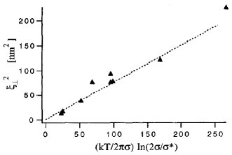
Refer to caption
(a) Experimental vertical roughness ξsubscript𝜉perpendicular-to\xi_{\perp} as a function of the expected curve for the case dominated by tension (lower line of table C.1).
Refer to caption
(b) Lateral correlation length as a function of the curve expected in the same limit (lower line of table C.1).
Figure C.1: Experimental correlation lengths as a function of the expected curves for the regime dominated by tension [84]. Note that the curves were traced under the assumption σr𝜎𝑟\sigma\approx r.

Besides, in this case, it is theoretically expected that ξsubscript𝜉perpendicular-to\xi_{\perp} relates to the mean separation from the substrate sdelimited-⟨⟩𝑠\langle s\rangle through [144]

2(ξσ)2=sσ+14ln(sσ).2superscriptsubscript𝜉perpendicular-tosubscript𝜎2delimited-⟨⟩𝑠subscript𝜎14delimited-⟨⟩𝑠subscript𝜎2\left(\frac{\xi_{\perp}}{\ell_{\sigma}}\right)^{2}=\frac{\langle s\rangle}{\ell_{\sigma}}+\frac{1}{4}\ln\left(\frac{\langle s\rangle}{\ell_{\sigma}}\right)\,. (C.6)

where σ=kBT/(2πσ)subscript𝜎subscript𝑘B𝑇2𝜋𝜎\ell_{\sigma}=\sqrt{k_{\mathrm{B}}T/(2\pi\sigma)}.

From eq.(C.5), the last equation of table C.1 and eq.(C.6), one obtains finally

Vsteric=bkBTσκ(σs)14esσ,subscript𝑉steric𝑏subscript𝑘B𝑇𝜎𝜅superscriptsubscript𝜎delimited-⟨⟩𝑠14superscript𝑒delimited-⟨⟩𝑠subscript𝜎V_{\mathrm{steric}}=b\,\frac{k_{\mathrm{B}}T\,\sigma}{\kappa}\left(\frac{\ell_{\sigma}}{\langle s\rangle}\right)^{\frac{1}{4}}e^{-\frac{\langle s\rangle}{\ell_{\sigma}}}\,, (C.7)

where b𝑏b is a dimensionless prefactor. One can see the plot of Vtotal=VvdW+Vsteric+Vgravsubscript𝑉totalsubscript𝑉vdWsubscript𝑉stericsubscript𝑉gravV_{\mathrm{total}}=V_{\mathrm{vdW}}+V_{\mathrm{steric}}+V_{\mathrm{grav}} for typical experimental values σ=1.7×10⁵N/m𝜎1.7superscript105Nm\sigma=1.7\times 10^{-5}\,\mathrm{N/m}, κ=35kBT𝜅35subscript𝑘B𝑇\kappa=35\,k_{\mathrm{B}}T, b=0.085𝑏0.085b=0.085, AH=2.6×10²¹Jsubscript𝐴𝐻2.6superscript1021JA_{H}=2.6\times 10^{-21}\,\mathrm{J}, DM=20μmsubscript𝐷𝑀20𝜇mD_{M}=20\,\mathrm{\mu m}, DA=10μmsubscript𝐷𝐴10𝜇mD_{A}=10\,\mathrm{\mu m}, Δρ=7kg/m3Δ𝜌7kgsuperscriptm3\Delta\rho=7\,\mathrm{kg/m^{3}} can be seen in Fig. 1.33(b).

Appendix D Determination of ξsubscript𝜉perpendicular-to\xi_{\perp} and ξsubscript𝜉parallel-to\xi_{\parallel} for planar membranes under a quadratic potential

In this section we derive the correlation length ξsubscript𝜉parallel-to\xi_{\parallel} and the roughness ξsubscript𝜉perpendicular-to\xi_{\perp} for a planar membrane under a quadratic potential [145][144]. Assuming that the Hamiltonian is given by eq.(1.38), the correlation function is given by

G(𝒓𝒓)=kBTAp𝒒ei𝒒(𝒓𝒓)V′′+σq2+κq4.𝐺𝒓superscript𝒓subscript𝑘B𝑇subscript𝐴𝑝subscript𝒒superscript𝑒𝑖𝒒𝒓superscript𝒓bold-′superscript𝑉′′𝜎superscript𝑞2𝜅superscript𝑞4G(\bm{r}-\bm{r}^{\prime})=\frac{k_{\mathrm{B}}T}{A_{p}}\sum_{\bm{q}}\frac{e^{i\,\bm{q}\cdot(\bm{r}-\bm{r^{\prime}})}}{V^{\prime\prime}+\sigma\,q^{2}+\kappa\,q^{4}}\,. (D.1)

By definition, one has

ξ2superscriptsubscript𝜉perpendicular-to2\displaystyle\xi_{\perp}^{2} =\displaystyle= h(𝒓)h(𝒓)delimited-⟨⟩𝒓𝒓\displaystyle\langle h(\bm{r})h(\bm{r})\rangle\, (D.2)
=\displaystyle= kBTAp𝒒1V′′+σq2+κq4,subscript𝑘B𝑇subscript𝐴𝑝subscript𝒒1superscript𝑉′′𝜎superscript𝑞2𝜅superscript𝑞4\displaystyle\frac{k_{\mathrm{B}}T}{A_{p}}\sum_{\bm{q}}\frac{1}{V^{\prime\prime}+\sigma\,q^{2}+\kappa\,q^{4}}\,,
=\displaystyle= kBTApqminqmaxd𝒒(2π)21V′′+σq2+κq4,subscript𝑘B𝑇subscript𝐴𝑝superscriptsubscriptsubscript𝑞minsubscript𝑞max𝑑𝒒superscript2𝜋21superscript𝑉′′𝜎superscript𝑞2𝜅superscript𝑞4\displaystyle\frac{k_{\mathrm{B}}T}{A_{p}}\int_{q_{\mathrm{min}}}^{q_{\mathrm{max}}}\frac{d\bm{q}}{(2\pi)^{2}}\frac{1}{V^{\prime\prime}+\sigma\,q^{2}+\kappa\,q^{4}}\,,
=\displaystyle= kBT2πσΩ(σσ),subscript𝑘B𝑇2𝜋𝜎Ω𝜎superscript𝜎\displaystyle\frac{k_{\mathrm{B}}T}{2\pi\sigma}\,\Omega\left(\frac{\sigma}{\sigma^{*}}\right)\,,

where the last step is justified for very large Apsubscript𝐴𝑝A_{p} and for σa2/κ1much-less-than𝜎superscript𝑎2𝜅1\sigma a^{2}/\kappa\ll 1 (a𝑎a is a microscopical cut-off of order of the membrane thickness). The crossover tension σ=4κV′′superscript𝜎4𝜅superscript𝑉′′\sigma^{*}=\sqrt{4\,\kappa\,V^{\prime\prime}} defines two limits: one dominated by tension (σ>σ𝜎superscript𝜎\sigma>\sigma^{*}) and one dominated by the rigidity (σ<σ𝜎superscript𝜎\sigma<\sigma^{*}). The function ΩΩ\Omega is given explicitly by

Ω(y)={tan1(y21)y21fory<1,tanh1(1y2)1y2fory>1.Ω𝑦casessuperscript1superscript𝑦21superscript𝑦21for𝑦1missing-subexpressionmissing-subexpressionmissing-subexpressionsuperscript11superscript𝑦21superscript𝑦2for𝑦1\Omega(y)=\left\{\begin{array}[]{ccc}\frac{\tan^{-1}\left(\sqrt{y^{-2}-1}\right)}{\sqrt{y^{-2}-1}}&$for$&\,y<1\,,\\ \\ \frac{\tanh^{-1}\left(\sqrt{1-y^{-2}}\right)}{\sqrt{1-y^{-2}}}&$for$&\,y>1\,.\end{array}\right. (D.3)

To estimate ξsubscript𝜉parallel-to\xi_{\parallel}, one must evaluate the general correlation function

h(𝒓)h(0)delimited-⟨⟩𝒓0\displaystyle\langle h(\bm{r})h(0)\rangle =\displaystyle= kBTAp𝒒ei𝒒𝒓V′′+σq2+κq4,subscript𝑘B𝑇subscript𝐴𝑝subscript𝒒superscript𝑒𝑖𝒒𝒓superscript𝑉′′𝜎superscript𝑞2𝜅superscript𝑞4\displaystyle\frac{k_{\mathrm{B}}T}{A_{p}}\sum_{\bm{q}}\frac{e^{i\bm{q}\cdot\bm{r}}}{V^{\prime\prime}+\sigma\,q^{2}+\kappa\,q^{4}}\,, (D.4)
=\displaystyle= kBTApqminqmaxd𝒒(2π)2ei𝒒𝒓V′′+σq2+κq4,subscript𝑘B𝑇subscript𝐴𝑝superscriptsubscriptsubscript𝑞𝑚𝑖𝑛subscript𝑞𝑚𝑎𝑥𝑑𝒒superscript2𝜋2superscript𝑒𝑖𝒒𝒓superscript𝑉′′𝜎superscript𝑞2𝜅superscript𝑞4\displaystyle\frac{k_{\mathrm{B}}T}{A_{p}}\int_{q_{min}}^{q_{max}}\frac{d\bm{q}}{(2\pi)^{2}}\frac{e^{i\bm{q}\cdot\bm{r}}}{V^{\prime\prime}+\sigma\,q^{2}+\kappa\,q^{4}}\,,
=\displaystyle= kBTApqminqmaxdq(2π)qJ0(qr)V′′+σq2+κq4,subscript𝑘B𝑇subscript𝐴𝑝superscriptsubscriptsubscript𝑞𝑚𝑖𝑛subscript𝑞𝑚𝑎𝑥𝑑𝑞2𝜋𝑞subscript𝐽0𝑞𝑟superscript𝑉′′𝜎superscript𝑞2𝜅superscript𝑞4\displaystyle\frac{k_{\mathrm{B}}T}{A_{p}}\int_{q_{min}}^{q_{max}}\frac{dq}{(2\pi)}\frac{q\,J_{0}(qr)}{V^{\prime\prime}+\sigma\,q^{2}+\kappa\,q^{4}}\,,

where J0(x)subscript𝐽0𝑥J_{0}(x) is the Bessel function of the first kind and of order 00 and compare its asymptotic behavior with ξ2er/ξsuperscriptsubscript𝜉perpendicular-to2superscript𝑒𝑟subscript𝜉parallel-to\xi_{\perp}^{2}e^{-r/\xi_{\parallel}}.

The results coming from eq.(D.2) and eq.(D.4) for the two limiting situations are summed up in table D.1.

Case ξ2superscriptsubscript𝜉perpendicular-to2\xi_{\perp}^{2} ξsubscript𝜉parallel-to\xi_{\parallel} Relation
σ<σ𝜎superscript𝜎\sigma<\sigma^{*} kBT8κV′′subscript𝑘B𝑇8𝜅superscript𝑉′′\frac{k_{\mathrm{B}}T}{8\sqrt{\kappa V^{\prime\prime}}} (4κV′′)14superscript4𝜅superscript𝑉′′14\left(\frac{4\kappa}{V^{\prime\prime}}\right)^{\frac{1}{4}} ξ2kBT16κξ2superscriptsubscript𝜉perpendicular-to2subscript𝑘B𝑇16𝜅superscriptsubscript𝜉parallel-to2\xi_{\perp}^{2}\approx\frac{k_{\mathrm{B}}T}{16\kappa}\xi_{\parallel}^{2}
σ>σ𝜎superscript𝜎\sigma>\sigma^{*} kBT2πσln(2σσ)subscript𝑘B𝑇2𝜋𝜎2𝜎superscript𝜎\frac{k_{\mathrm{B}}T}{2\pi\sigma}\ln\left(\frac{2\sigma}{\sigma^{*}}\right) (σV′′)12superscript𝜎superscript𝑉′′12\left(\frac{\sigma}{V^{\prime\prime}}\right)^{\frac{1}{2}} ξ2kBT4πσln(σξ2κ)superscriptsubscript𝜉perpendicular-to2subscript𝑘B𝑇4𝜋𝜎𝜎superscriptsubscript𝜉parallel-to2𝜅\xi_{\perp}^{2}\approx\frac{k_{\mathrm{B}}T}{4\pi\sigma}\ln\left(\frac{\sigma\,\xi_{\parallel}^{2}}{\kappa}\right)
Table D.1: Theoretical previsions for ξsubscript𝜉perpendicular-to\xi_{\perp} and ξsubscript𝜉parallel-to\xi_{\parallel} as a function of σ𝜎\sigma, κ𝜅\kappa and V′′superscript𝑉′′V^{\prime\prime}. The last column is obtained by substituting the third column on the second.

Appendix E Verification of the projected stress tensor in spherical geometry: the planar limit

In order to check the expressions given in eqs.(4.2)-(4.2), we consider the limit R𝑅R\rightarrow\infty, which should yield the projected stress tensor for a flat membrane given in section 1.5.2. We consider a general point (θ,ϕ)𝜃italic-ϕ(\theta,\phi) on the sphere and we define a local system of Cartesian coordinates (x,y,z)𝑥𝑦𝑧(x,y,z), such that dx=Rdθ𝑑𝑥𝑅𝑑𝜃dx=Rd\theta, dy=Rsinθdϕ𝑑𝑦𝑅𝜃𝑑italic-ϕdy=R\sin\theta d\phi and dz=dr𝑑𝑧𝑑𝑟dz=dr. We want to determine the projected stress tensor 𝚺superscript𝚺\bm{\Sigma}^{\prime} in these new coordinates. The component of the elementary force dfα𝑑subscript𝑓𝛼df_{\alpha} along a general direction α{x,y,z}𝛼𝑥𝑦𝑧\alpha\in\{x,y,z\} exerted through a cut perpendicular to x𝑥x reads dfα=Σαxd=Σαθdϕ𝑑subscript𝑓𝛼superscriptsubscriptΣ𝛼𝑥𝑑subscriptΣ𝛼𝜃𝑑italic-ϕdf_{\alpha}=\Sigma_{\alpha x}^{\prime}\,d\ell=\Sigma_{\alpha\theta}\,d\phi, with the correspondence d=Rsinθdϕ𝑑𝑅𝜃𝑑italic-ϕd\ell=R\sin\theta\,d\phi. Thus we have Σαx=Σαθ/(Rsinθ)superscriptsubscriptΣ𝛼𝑥subscriptΣ𝛼𝜃𝑅𝜃\Sigma_{\alpha x}^{\prime}=\Sigma_{\alpha\theta}/(R\sin\theta). Likewise, Σαy=Σαϕ/RsuperscriptsubscriptΣ𝛼𝑦subscriptΣ𝛼italic-ϕ𝑅\Sigma_{\alpha y}^{\prime}=\Sigma_{\alpha\phi}/R, since in this case d=Rdθ𝑑𝑅𝑑𝜃d\ell=R\,d\theta. In the limit of large R𝑅R, the plane tangent to the sphere at the point (θ,ϕ)𝜃italic-ϕ(\theta,\phi) becomes the reference plane of the membrane, and the height of the membrane over this plane is h(x,y)=Ru(θ,ϕ)𝑥𝑦𝑅𝑢𝜃italic-ϕh(x,y)=R\,u(\theta,\phi). Hence uθ=Rux=hxsubscript𝑢𝜃𝑅subscript𝑢𝑥subscript𝑥u_{\theta}=R\,u_{x}=h_{x}, uϕ=Rsinθuy=sinθhysubscript𝑢italic-ϕ𝑅𝜃subscript𝑢𝑦𝜃subscript𝑦u_{\phi}=R\,\sin\theta\,u_{y}=\sin\theta\,h_{y}, uθθ=R2uxx=Rhxxsubscript𝑢𝜃𝜃superscript𝑅2subscript𝑢𝑥𝑥𝑅subscript𝑥𝑥u_{\theta\theta}=R^{2}\,u_{xx}=R\,h_{xx}, uϕϕ=R2sin2θuyy=Rsin2θhyysubscript𝑢italic-ϕitalic-ϕsuperscript𝑅2superscript2𝜃subscript𝑢𝑦𝑦𝑅superscript2𝜃subscript𝑦𝑦u_{\phi\phi}=R^{2}\sin^{2}\theta\,u_{yy}=R\,\sin^{2}\theta\,h_{yy}, etc. Keeping the terms that are dominant in the limit R𝑅R\rightarrow\infty, we obtain

ΣxxsuperscriptsubscriptΣ𝑥𝑥\displaystyle\Sigma_{xx}^{\prime} =\displaystyle= σ+σ2(hy2hx2)+κ2(hyy2hxx2)+κhxx2h,𝜎𝜎2subscriptsuperscript2𝑦subscriptsuperscript2𝑥𝜅2subscriptsuperscript2𝑦𝑦subscriptsuperscript2𝑥𝑥𝜅subscript𝑥subscript𝑥superscript2\displaystyle\sigma+\frac{\sigma}{2}\left({h^{2}_{y}-h^{2}_{x}}\right)+\frac{\kappa}{2}\left({h^{2}_{yy}-h^{2}_{xx}}\right)+\kappa h_{x}\partial_{x}\nabla^{2}h\,, (E.1)
ΣyxsuperscriptsubscriptΣ𝑦𝑥\displaystyle\Sigma_{yx}^{\prime} =\displaystyle= σhxhyκhxy2h+κhyx2h,𝜎subscript𝑥subscript𝑦𝜅subscript𝑥𝑦superscript2𝜅subscript𝑦subscript𝑥superscript2\displaystyle-\sigma h_{x}h_{y}-\kappa h_{xy}\nabla^{2}h+\kappa h_{y}\partial_{x}\nabla^{2}h, (E.2)
ΣrxsuperscriptsubscriptΣ𝑟𝑥\displaystyle\Sigma_{rx}^{\prime} =\displaystyle= σhxκx2h,𝜎subscript𝑥𝜅subscript𝑥superscript2\displaystyle\sigma h_{x}-\kappa\partial_{x}\nabla^{2}h, (E.3)
ΣyysuperscriptsubscriptΣ𝑦𝑦\displaystyle\Sigma_{yy}^{\prime} =\displaystyle= σ+σ2(hx2hy2)+κ2(hxx2hyy2)+κhyy2h,𝜎𝜎2subscriptsuperscript2𝑥subscriptsuperscript2𝑦𝜅2subscriptsuperscript2𝑥𝑥subscriptsuperscript2𝑦𝑦𝜅subscript𝑦subscript𝑦superscript2\displaystyle\sigma+\frac{\sigma}{2}\left({h^{2}_{x}-h^{2}_{y}}\right)+\frac{\kappa}{2}\left({h^{2}_{xx}-h^{2}_{yy}}\right)+\kappa h_{y}\partial_{y}\nabla^{2}h\,, (E.4)
ΣxysuperscriptsubscriptΣ𝑥𝑦\displaystyle\Sigma_{xy}^{\prime} =\displaystyle= σhxhyκhxy2h+κhxy2h,𝜎subscript𝑥subscript𝑦𝜅subscript𝑥𝑦superscript2𝜅subscript𝑥subscript𝑦superscript2\displaystyle-\sigma h_{x}h_{y}-\kappa h_{xy}\nabla^{2}h+\kappa h_{x}\partial_{y}\nabla^{2}h, (E.5)
ΣrysuperscriptsubscriptΣ𝑟𝑦\displaystyle\Sigma_{ry}^{\prime} =\displaystyle= σhyκy2h,𝜎subscript𝑦𝜅subscript𝑦superscript2\displaystyle\sigma h_{y}-\kappa\partial_{y}\nabla^{2}h, (E.6)

which agree with the results of section 1.5.2.

Appendix F Correlation functions for vesicles and their relationship

There are five fundamental correlation functions, which we have calculated explicitly:

uϕ2delimited-⟨⟩superscriptsubscript𝑢italic-ϕ2\displaystyle\left<{u_{\phi}^{2}}\right> =\displaystyle= ω,ωϕYlm(θ,ϕ)ϕYlm(θ,ϕ)ulmulm,subscript𝜔superscript𝜔subscriptitalic-ϕsuperscriptsubscript𝑌𝑙𝑚𝜃italic-ϕsubscriptitalic-ϕsuperscriptsubscript𝑌superscript𝑙superscript𝑚𝜃italic-ϕdelimited-⟨⟩subscript𝑢𝑙𝑚subscript𝑢superscript𝑙superscript𝑚\displaystyle\sum_{\omega,\omega^{\prime}}\partial_{\phi}Y_{l}^{m}(\theta,\phi)\partial_{\phi}Y_{l^{\prime}}^{m^{\prime}}(\theta,\phi)\left<{u_{lm}u_{l^{\prime}m^{\prime}}}\right>\,, (F.1)
=\displaystyle= ωkBTH~lϕYlmϕ(Ylm)=ωkBTH~lm2|Ylm|2,subscript𝜔subscript𝑘𝐵𝑇subscript~𝐻𝑙subscriptitalic-ϕsuperscriptsubscript𝑌𝑙𝑚subscriptitalic-ϕsuperscriptsuperscriptsubscript𝑌𝑙𝑚subscript𝜔subscript𝑘𝐵𝑇subscript~𝐻𝑙superscript𝑚2superscriptsuperscriptsubscript𝑌𝑙𝑚2\displaystyle\sum_{\omega}\frac{k_{B}T}{\widetilde{H}_{l}}\partial_{\phi}Y_{l}^{m}\partial_{\phi}\left({Y_{l}^{m}}\right)^{*}=\sum_{\omega}\frac{k_{B}T}{\widetilde{H}_{l}}m^{2}|Y_{l}^{m}|^{2}\,,
=\displaystyle= sin2θkBT4πl=2l(l+1)(2l+1)2H~lsuperscript2𝜃subscript𝑘𝐵𝑇4𝜋subscript𝑙2𝑙𝑙12𝑙12subscript~𝐻𝑙\displaystyle\sin^{2}\theta\,\frac{k_{B}T}{4\pi}\sum_{l=2}\frac{l(l+1)(2l+1)}{2\widetilde{H}_{l}}
uϕϕ2delimited-⟨⟩superscriptsubscript𝑢italic-ϕitalic-ϕ2\displaystyle\left<{u_{\phi\phi}^{2}}\right> =\displaystyle= ωkBTH~lm4|Ylm|2,subscript𝜔subscript𝑘𝐵𝑇subscript~𝐻𝑙superscript𝑚4superscriptsuperscriptsubscript𝑌𝑙𝑚2\displaystyle\sum_{\omega}\frac{k_{B}T}{\widetilde{H}_{l}}\,m^{4}|Y_{l}^{m}|^{2}\,, (F.2)
=\displaystyle= sin2θkBT4πl=2l(l+1)(2l+1)8H~l[4+3(2+l+l2)sin2θ],superscript2𝜃subscript𝑘𝐵𝑇4𝜋subscript𝑙2𝑙𝑙12𝑙18subscript~𝐻𝑙delimited-[]432𝑙superscript𝑙2superscript2𝜃\displaystyle\sin^{2}\theta\frac{k_{B}T}{4\pi}\sum_{l=2}\frac{l(l+1)(2l+1)}{8\widetilde{H}_{l}}\Big{[}4+3(-2+l+l^{2})\sin^{2}\theta\Big{]}\,,
uθ2delimited-⟨⟩superscriptsubscript𝑢𝜃2\displaystyle\left<{u_{\theta}^{2}}\right> =\displaystyle= ωkBTH~lθYlmθ(Ylm)=kBT4πl=2l(l+1)(2l+1)2H~l,subscript𝜔subscript𝑘𝐵𝑇subscript~𝐻𝑙subscript𝜃superscriptsubscript𝑌𝑙𝑚subscript𝜃superscriptsuperscriptsubscript𝑌𝑙𝑚subscript𝑘𝐵𝑇4𝜋subscript𝑙2𝑙𝑙12𝑙12subscript~𝐻𝑙\displaystyle\sum_{\omega}\frac{k_{B}T}{\widetilde{H}_{l}}\,\partial_{\theta}Y_{l}^{m}\partial_{\theta}\left({Y_{l}^{m}}\right)^{*}=\frac{k_{B}T}{4\pi}\sum_{l=2}\frac{l(l+1)(2l+1)}{2\widetilde{H}_{l}}\,, (F.3)
uθθ2delimited-⟨⟩superscriptsubscript𝑢𝜃𝜃2\displaystyle\left<{u_{\theta\theta}^{2}}\right> =\displaystyle= ωkBTH~lθ2Ylmθ2(Ylm),subscript𝜔subscript𝑘𝐵𝑇subscript~𝐻𝑙superscriptsubscript𝜃2superscriptsubscript𝑌𝑙𝑚superscriptsubscript𝜃2superscriptsuperscriptsubscript𝑌𝑙𝑚\displaystyle\sum_{\omega}\frac{k_{B}T}{\widetilde{H}_{l}}\,\partial_{\theta}^{2}Y_{l}^{m}\partial_{\theta}^{2}\left({Y_{l}^{m}}\right)^{*}\,, (F.4)
=\displaystyle= kBT4πl=2l(l+1)(2l+1)(2+3l+3l2)8H~l,subscript𝑘𝐵𝑇4𝜋subscript𝑙2𝑙𝑙12𝑙123𝑙3superscript𝑙28subscript~𝐻𝑙\displaystyle\frac{k_{B}T}{4\pi}\sum_{l=2}\frac{l(l+1)(2l+1)(-2+3l+3l^{2})}{8\widetilde{H}_{l}}\,,
uθuθϕϕdelimited-⟨⟩subscript𝑢𝜃subscript𝑢𝜃italic-ϕitalic-ϕ\displaystyle\left<{u_{\theta}\,u_{\theta\phi\phi}}\right> =\displaystyle= ωkBTH~lm2θYlmθ(Ylm),subscript𝜔subscript𝑘𝐵𝑇subscript~𝐻𝑙superscript𝑚2subscript𝜃superscriptsubscript𝑌𝑙𝑚subscript𝜃superscriptsuperscriptsubscript𝑌𝑙𝑚\displaystyle-\sum_{\omega}\frac{k_{B}T}{\widetilde{H}_{l}}\,m^{2}\partial_{\theta}Y_{l}^{m}\partial_{\theta}\left({Y_{l}^{m}}\right)^{*}\,, (F.5)
=\displaystyle= kBT4πl=2l(l+1)(2l+1)2H~l[1+(l+3)(l2)4sin2θ].subscript𝑘𝐵𝑇4𝜋subscript𝑙2𝑙𝑙12𝑙12subscript~𝐻𝑙delimited-[]1𝑙3𝑙24superscript2𝜃\displaystyle-\frac{k_{B}T}{4\pi}\sum_{l=2}\frac{l(l+1)(2l+1)}{2\widetilde{H}_{l}}\left[{1+\frac{(l+3)(l-2)}{4}\sin^{2}\theta}\right]\,.

The other correlation functions either vanish or may be deduced from them. Remembering that ul,m=(1)mulmsubscript𝑢𝑙𝑚superscript1𝑚superscriptsubscript𝑢𝑙𝑚u_{l,-m}=(-1)^{m}u_{lm}^{*}, (Ylm)=(1)mYlmsuperscriptsuperscriptsubscript𝑌𝑙𝑚superscript1𝑚subscriptsuperscript𝑌𝑚𝑙\left({Y_{l}^{m}}\right)^{*}=(-1)^{m}Y^{-m}_{l} and

nYlm(θ,ϕ)ϕn=(im)nYlm(θ,ϕ),superscript𝑛superscriptsubscript𝑌𝑙𝑚𝜃italic-ϕsuperscriptitalic-ϕ𝑛superscript𝑖𝑚𝑛superscriptsubscript𝑌𝑙𝑚𝜃italic-ϕ\frac{\partial^{n}Y_{l}^{m}(\theta,\phi)}{\partial\phi^{n}}=(i\,m)^{n}\,Y_{l}^{m}(\theta,\phi)\,, (F.6)

one can demonstrate that

n+1Ylm(θ,ϕ)ϕn+1p1Ylm(θ,ϕ)ϕp1=nYlm(θ,ϕ)ϕnpYlm(θ,ϕ)ϕp,superscript𝑛1superscriptsubscript𝑌𝑙𝑚𝜃italic-ϕsuperscriptitalic-ϕ𝑛1superscript𝑝1superscriptsuperscriptsubscript𝑌𝑙𝑚𝜃italic-ϕsuperscriptitalic-ϕ𝑝1superscript𝑛superscriptsubscript𝑌𝑙𝑚𝜃italic-ϕsuperscriptitalic-ϕ𝑛superscript𝑝superscriptsuperscriptsubscript𝑌𝑙𝑚𝜃italic-ϕsuperscriptitalic-ϕ𝑝\frac{\partial^{n+1}{Y_{l}^{m}}(\theta,\phi)}{\partial\phi^{n+1}}\frac{\partial^{p-1}{Y_{l}^{m}}^{*}(\theta,\phi)}{\partial\phi^{p-1}}=-\frac{\partial^{n}{Y_{l}^{m}}(\theta,\phi)}{\partial\phi^{n}}\frac{\partial^{p}{Y_{l}^{m}}^{*}(\theta,\phi)}{\partial\phi^{p}}\,, (F.7)

which holds also in the presence of derivatives with respect to θ𝜃\theta. From this relation, one deduces the following rule: when averaging the product of two terms, one may pass a derivative with respect to ϕitalic-ϕ\phi from one term to the other while multiplying by 11-1. Hence,

uϕ2delimited-⟨⟩superscriptsubscript𝑢italic-ϕ2\displaystyle\langle u_{\phi}^{2}\rangle =\displaystyle= uuϕϕ,delimited-⟨⟩𝑢subscript𝑢italic-ϕitalic-ϕ\displaystyle-\langle u\,u_{\phi\phi}\rangle\,, (F.8)
uϕuθdelimited-⟨⟩subscript𝑢italic-ϕsubscript𝑢𝜃\displaystyle\langle u_{\phi}\,u_{\theta}\rangle =\displaystyle= uuϕθ,delimited-⟨⟩𝑢subscript𝑢italic-ϕ𝜃\displaystyle-\langle u\,u_{\phi\theta}\rangle\,, (F.9)
uϕuθθdelimited-⟨⟩subscript𝑢italic-ϕsubscript𝑢𝜃𝜃\displaystyle\langle u_{\phi}\,u_{\theta\theta}\rangle =\displaystyle= uθuϕθ.delimited-⟨⟩subscript𝑢𝜃subscript𝑢italic-ϕ𝜃\displaystyle-\langle u_{\theta}\,u_{\phi\theta}\rangle\,. (F.10)

Consequently, averages implying an odd number of derivatives with respect to ϕitalic-ϕ\phi vanish:

uuϕdelimited-⟨⟩𝑢subscript𝑢italic-ϕ\displaystyle\langle u\,u_{\phi}\rangle =\displaystyle= 0,0\displaystyle 0\,, (F.11)
uθuϕdelimited-⟨⟩subscript𝑢𝜃subscript𝑢italic-ϕ\displaystyle\langle u_{\theta}\,u_{\phi}\rangle =\displaystyle= 0,0\displaystyle 0\,, (F.12)
uϕuϕϕdelimited-⟨⟩subscript𝑢italic-ϕsubscript𝑢italic-ϕitalic-ϕ\displaystyle\langle u_{\phi}\,u_{\phi\phi}\rangle =\displaystyle= 0,0\displaystyle 0\,, (F.13)
uθuθϕdelimited-⟨⟩subscript𝑢𝜃subscript𝑢𝜃italic-ϕ\displaystyle\langle u_{\theta}\,u_{\theta\phi}\rangle =\displaystyle= 0,0\displaystyle 0\,, (F.14)
uθθuθϕdelimited-⟨⟩subscript𝑢𝜃𝜃subscript𝑢𝜃italic-ϕ\displaystyle\langle u_{\theta\theta}\,u_{\theta\phi}\rangle =\displaystyle= 0,0\displaystyle 0\,, (F.15)
uϕϕuθϕdelimited-⟨⟩subscript𝑢italic-ϕitalic-ϕsubscript𝑢𝜃italic-ϕ\displaystyle\langle u_{\phi\phi}\,u_{\theta\phi}\rangle =\displaystyle= 0.0\displaystyle 0\,. (F.16)

Another very helpful relation is the addition theorem for spherical harmonics:

m=llYlm(θ1,ϕ)Ylm(θ2,ϕ)=2l+14πPl(cos(γ)),superscriptsubscript𝑚𝑙𝑙superscriptsubscript𝑌𝑙𝑚subscript𝜃1italic-ϕsuperscriptsuperscriptsubscript𝑌𝑙𝑚subscript𝜃2italic-ϕ2𝑙14𝜋subscript𝑃𝑙𝛾\sum_{m=-l}^{l}Y_{l}^{m}(\theta_{1},\phi){Y_{l}^{m}}^{*}(\theta_{2},\phi)=\frac{2l+1}{4\pi}P_{l}(\cos(\gamma))\,, (F.17)

where Plsubscript𝑃𝑙P_{l} is the Legendre polynomial of order l𝑙l and γ=θ2θ1𝛾subscript𝜃2subscript𝜃1\gamma=\theta_{2}-\theta_{1}. By differentiating this relation k𝑘k times with respect to θ1subscript𝜃1\theta_{1} and p𝑝p times with respect to θ2subscript𝜃2\theta_{2}, one obtains

m=llkYlm(θ1,ϕ)θ1kpYlm(θ2,ϕ)θ2p=(1)k(2l+1)4πdk+pPl(cos(γ))dγk+p.superscriptsubscript𝑚𝑙𝑙superscript𝑘superscriptsubscript𝑌𝑙𝑚subscript𝜃1italic-ϕsuperscriptsubscript𝜃1𝑘superscript𝑝superscriptsuperscriptsubscript𝑌𝑙𝑚subscript𝜃2italic-ϕsuperscriptsubscript𝜃2𝑝superscript1𝑘2𝑙14𝜋superscript𝑑𝑘𝑝subscript𝑃𝑙𝛾𝑑superscript𝛾𝑘𝑝\sum_{m=-l}^{l}\frac{\partial^{k}Y_{l}^{m}(\theta_{1},\phi)}{\partial\theta_{1}^{k}}\frac{\partial^{p}{Y_{l}^{m}}^{*}(\theta_{2},\phi)}{\partial\theta_{2}^{p}}=(-1)^{k}\frac{(2l+1)}{4\pi}\frac{d^{k+p}P_{l}(\cos(\gamma))}{d\gamma^{k+p}}\,. (F.18)

In particular, for θ1=θ2=θsubscript𝜃1subscript𝜃2𝜃\theta_{1}=\theta_{2}=\theta, we have

m=llkYlm(θ,ϕ)θkpYlm(θ,ϕ)θp=(1)k(2l+1)4πdk+pPl(1)dγk+p.superscriptsubscript𝑚𝑙𝑙superscript𝑘superscriptsubscript𝑌𝑙𝑚𝜃italic-ϕsuperscript𝜃𝑘superscript𝑝superscriptsuperscriptsubscript𝑌𝑙𝑚𝜃italic-ϕsuperscript𝜃𝑝superscript1𝑘2𝑙14𝜋superscript𝑑𝑘𝑝subscript𝑃𝑙1𝑑superscript𝛾𝑘𝑝\sum_{m=-l}^{l}\frac{\partial^{k}Y_{l}^{m}(\theta,\phi)}{\partial\theta^{k}}\frac{\partial^{p}{Y_{l}^{m}}^{*}(\theta,\phi)}{\partial\theta^{p}}=(-1)^{k}\frac{(2l+1)}{4\pi}\frac{d^{k+p}P_{l}(1)}{d\gamma^{k+p}}\,. (F.19)

Inversely, one can differentiate eq.(F.17) p𝑝p times with respect to θ1subscript𝜃1\theta_{1} and k𝑘k times with respect to θ2subscript𝜃2\theta_{2}, and then make θ1=θ2=θsubscript𝜃1subscript𝜃2𝜃\theta_{1}=\theta_{2}=\theta, which yields

m=llpYlm(θ,ϕ)θpkYlm(θ,ϕ)θk=(1)p(2l+1)4πdk+pPl(1)dγk+p.superscriptsubscript𝑚𝑙𝑙superscript𝑝superscriptsubscript𝑌𝑙𝑚𝜃italic-ϕsuperscript𝜃𝑝superscript𝑘superscriptsuperscriptsubscript𝑌𝑙𝑚𝜃italic-ϕsuperscript𝜃𝑘superscript1𝑝2𝑙14𝜋superscript𝑑𝑘𝑝subscript𝑃𝑙1𝑑superscript𝛾𝑘𝑝\sum_{m=-l}^{l}\frac{\partial^{p}Y_{l}^{m}(\theta,\phi)}{\partial\theta^{p}}\frac{\partial^{k}{Y_{l}^{m}}^{*}(\theta,\phi)}{\partial\theta^{k}}=(-1)^{p}\frac{(2l+1)}{4\pi}\frac{d^{k+p}P_{l}(1)}{d\gamma^{k+p}}\,. (F.20)

For θ1=θ2subscript𝜃1subscript𝜃2\theta_{1}=\theta_{2}, we can exchange k𝑘k and p𝑝p and thus eq.(F.19) must be equal to eq.(F.20). Accordingly, the sum

m=llkYlm(θ,ϕ)θkpYlm(θ,ϕ)θpsuperscriptsubscript𝑚𝑙𝑙superscript𝑘superscriptsubscript𝑌𝑙𝑚𝜃italic-ϕsuperscript𝜃𝑘superscript𝑝superscriptsubscript𝑌𝑙𝑚superscript𝜃italic-ϕsuperscript𝜃𝑝\sum_{m=-l}^{l}\frac{\partial^{k}Y_{l}^{m}(\theta,\phi)}{\partial\theta^{k}}\frac{\partial^{p}Y_{l}^{m}(\theta,\phi)^{*}}{\partial\theta^{p}} (F.21)

vanishes for k+p𝑘𝑝k+p odd, implying:

uuθdelimited-⟨⟩𝑢subscript𝑢𝜃\displaystyle\langle u\,u_{\theta}\rangle =\displaystyle= 0,0\displaystyle 0\,, (F.22)
uuθθθdelimited-⟨⟩𝑢subscript𝑢𝜃𝜃𝜃\displaystyle\langle u\,u_{\theta\theta\theta}\rangle =\displaystyle= 0.0\displaystyle 0\,. (F.23)

Note that this does not hold when derivations with respect to ϕitalic-ϕ\phi are also involved.

Starting again from the addition theorem, one may show that

m=llk+1Ylm(θ,ϕ)θk+1p1Ylm(θ,ϕ)θp1=m=llkYlm(θ,ϕ)θkpYlm(θ,ϕ)θp.superscriptsubscript𝑚𝑙𝑙superscript𝑘1superscriptsubscript𝑌𝑙𝑚𝜃italic-ϕsuperscript𝜃𝑘1superscript𝑝1superscriptsuperscriptsubscript𝑌𝑙𝑚𝜃italic-ϕsuperscript𝜃𝑝1superscriptsubscript𝑚𝑙𝑙superscript𝑘superscriptsubscript𝑌𝑙𝑚𝜃italic-ϕsuperscript𝜃𝑘superscript𝑝superscriptsuperscriptsubscript𝑌𝑙𝑚𝜃italic-ϕsuperscript𝜃𝑝\sum_{m=-l}^{l}\frac{\partial^{k+1}Y_{l}^{m}(\theta,\phi)}{\partial\theta^{k+1}}\frac{\partial^{p-1}{Y_{l}^{m}}^{*}(\theta,\phi)}{\partial\theta^{p-1}}=-\sum_{m=-l}^{l}\frac{\partial^{k}Y_{l}^{m}(\theta,\phi)}{\partial\theta^{k}}\frac{\partial^{p}{Y_{l}^{m}}^{*}(\theta,\phi)}{\partial\theta^{p}}\,. (F.24)

It follows that, when averaging the product of two terms, one may pass the derivative on θ𝜃\theta from one term to the other while multiplying by 11-1. This holds only, however, in the absence of derivatives with respect to ϕitalic-ϕ\phi. As a consequence

uθuθdelimited-⟨⟩subscript𝑢𝜃subscript𝑢𝜃\displaystyle\langle u_{\theta}\,u_{\theta}\rangle =\displaystyle= uuθθ,delimited-⟨⟩𝑢subscript𝑢𝜃𝜃\displaystyle-\langle u\,u_{\theta\theta}\rangle\,, (F.25)
uθuθθθdelimited-⟨⟩subscript𝑢𝜃subscript𝑢𝜃𝜃𝜃\displaystyle\langle u_{\theta}\,u_{\theta\theta\theta}\rangle =\displaystyle= uθθuθθ.delimited-⟨⟩subscript𝑢𝜃𝜃subscript𝑢𝜃𝜃\displaystyle-\langle u_{\theta\theta}\,u_{\theta\theta}\rangle\,. (F.26)

Finally, one may also use the fact that ΔYlm(θ,ϕ)=0Δsuperscriptsubscript𝑌𝑙𝑚𝜃italic-ϕ0\Delta Y_{l}^{m}(\theta,\phi)=0, where ΔΔ\Delta is the Laplacian in spherical coordinates, to obtain

uθuθθ=cotθuuθθcsc2θuθuϕϕ.delimited-⟨⟩subscript𝑢𝜃subscript𝑢𝜃𝜃𝜃delimited-⟨⟩𝑢subscript𝑢𝜃𝜃superscript2𝜃delimited-⟨⟩subscript𝑢𝜃subscript𝑢italic-ϕitalic-ϕ\langle u_{\theta}\,u_{\theta\theta}\rangle=\cot\theta\langle u\,u_{\theta\theta}\rangle-\csc^{2}\theta\langle u_{\theta}\,u_{\phi\phi}\rangle\,. (F.27)

Since uθuθθdelimited-⟨⟩subscript𝑢𝜃subscript𝑢𝜃𝜃\langle u_{\theta}u_{\theta\theta}\rangle vanishes, one obtains

uθuϕϕ=sinθcosθuθ2.delimited-⟨⟩subscript𝑢𝜃subscript𝑢italic-ϕitalic-ϕ𝜃𝜃delimited-⟨⟩superscriptsubscript𝑢𝜃2\langle u_{\theta}\,u_{\phi\phi}\rangle=-\sin\theta\cos\theta\,\langle u_{\theta}^{2}\rangle\,. (F.28)

In conclusion, eqs.(F.1)-(F.5), together with eqs.(F.8)–(F.16), eqs.(F.22)–(F.23) and eq.(F.28) give all the correlations needed to evaluate 𝚺delimited-⟨⟩𝚺\langle\bm{\Sigma}\rangle.

References

  • [1] J. B. FOURNIER and C. BARBETTA. Direct calculation from the stress tensor of the lateral surface tension of fluctuating fluid membranes. Physical review letters, 100(7):78103, 2008.
  • [2] W. CAI et al. Measure factors, tension and correlations of fluid membranes. J. Phys. II France, 4:931–949, 1994.
  • [3] A. IMPARATO. Surface tension in bilayer membranes with fixed projected area. The Journal of Chemical Physics, 124:154714, 2006.
  • [4] J.-B. FOURNIER. On the stress and torque tensor in fluid membranes. Soft Matter, 3:883–888, 2007.
  • [5] C. BARBETTA et al. On the surface tension of fluctuating quasi-spherical vesicles. Eur. Phys. J. E, 31(3):333–342, 2010.
  • [6] C. BARBETTA and J.B. FOURNIER. On the fluctuations of the force exerted by a lipid nanotubule. The European Physical Journal E: Soft Matter and Biological Physics, 29(2):183–189, 2009.
  • [7] J.-B. FOURNIER and P. GALATOLA. Critical Fluctuations of Tense Fluid Membrane Tubules. Physical review letters, 98(1):18103, 2007.
  • [8] J. R. BAKER. The cell-theory: a restatement, history, and critique. Quarterly Journal of Microscopical Science, 93:157–190, 1952.
  • [9] J. D. ROBERTSON. Membrane structure. The Journal of Cell Biology, 91:189–204, 1981.
  • [10] M. EDIDIN. Lipids on the frontier: a century of cell-membrane bilayer. Nature, 4:414–418, 2003.
  • [11] T. HEIMBURG. Thermal biophysics of membranes. Wiley, 2007.
  • [12] B. ALBERTS et al. Molecular Biology of the Cell. Garland Science, 5th edition, 2008.
  • [13] G. EKNOYAN. Sir William Bowman: his contributions to the physiology and nephrology. Kidney International, 50:2120–2128, 1996.
  • [14] W. BOWMAN. On the minute structure and movements of voluntary muscle. Philos. Trans. R. Soc. Lond., 130:457–501, 1840.
  • [15] E. OVERTON. The probable origin and physiological significance of cellular osmotic properties. Vierteljahrschrift der Naturfoschende Gesselschaft (Zurich), 44:88–135, 1899.
  • [16] O. MOURITSEN. Life as a matter of fat. Springer, 2005.
  • [17] H. FRICKE. The electric capacity of suspensions with special reference to blood. Journal of General Physiology, pages 137–152, 1925.
  • [18] J. D. ROBERTSON. The ultrastructure of cell membranes and their derivatives. Biochem. Soc. Symp., 16:3–43, 1959.
  • [19] E. GORTER and F. GRENDEL. On bimolecular layers of lipoids on the chromocytes of the blood. J. Exp. Med., 41(4):439–443, 1925.
  • [20] M. BALLAND et al. Power laws in microrheology experiments on living cells: Comparative analysis and modeling. Phys. Rev. E, 74:21911, 2006.
  • [21] K. S. COLE. Surface forces of the arbacia egg. J. Cell. Comp. Physiol., 1:1–9, 1932.
  • [22] F. D. DANIELLI and E. N. HARVEY. The tension at the surface of mackerel egg oil, with remarks on the nature of the cell surface. J. Cell. Comp. Physiol., 5:483–494, 1934.
  • [23] F. D. DANIELLI and H. DAVSON. A contribution to the theory of permeability of thin films. J. Cell. Comp. Physiol., 5:495–508, 1935.
  • [24] W. BLOOM and D. W. FAWCETT. A Textbook of histology. Hodder Arnold, 12th edition, 1994.
  • [25] D. BRANTON. Fracture faces of frozen membranes. PNAS, 55:1048–1056, 1966.
  • [26] P. da SILVA and D. BRANTON. Membrane splitting in freeze-etching: covalently bound ferritin as a membrane marker. J. Cell Biol., 45:598–605, 1970.
  • [27] L. D. FRYE and M. EDIDIN. The rapid intermixing of cell surface antigens after formation of mouse-human heterokaryons. J. Cell Sci., 7:319–335, 1970.
  • [28] J. E. ROTHMANN and J. LENARD. Membrane asymmetry. Science, 195:743–753, 1997.
  • [29] K. SIMONS and G. VAN MEER. Lipid sorting in epithelial cells. Biochemistry, 12:6197–6202, 1988.
  • [30] M. EDIDIN. Lipid microdomains in cell surface membranes. Current Opinion in Structural Biology, 7:528–532, 1997.
  • [31] D. M. ENGELMAN. Membranes are more mosaic than fluid. Nature, 438:578–580, 2005.
  • [32] T. G. D’ONOFRIO et al. Controlling and measuring the interdependence of local properties of biomembranes. Langmuir, 19:1618–1623, 2003.
  • [33] P. F. F. ALMEIDA et al. Lateral diffusion in the liquid phases of dimyristoylphosphatidylcholine/cholesterol lipid bilayers: a free volume analysis. Biochemistry, 31:6739–6747, 1992.
  • [34] S. L. VEATCH and S. L. KELLER. Separation of liquid phases in giant vesicles of ternary mixtures of lipids and cholesterol. Biophysical Journal, 85:3074–3083, 2003.
  • [35] A. KUSUMI and J. S. HYDE. Spin-label saturation-transfer electron spin resonance detection of transient association of rhodopsin in reconstituted membranes. Biochemistry, 21:5978–5983, 1982.
  • [36] M. J. SAXTON and K. JACOBSON. Single particle tracking: application to membrane dynamics. Annu. Rev. Biophys. Biomol. Struct., 26:373–399, 1997.
  • [37] A. KUSUMI et al. Confined lateral diffusion of membrane receptors as studied by single particle tracking (nanovid microscopy). Effects of calcium-induced differentiation in cultured epithelial cells. Biophysical Journal, 65:2021–2040, 1993.
  • [38] M. B. FORSTNER et al. Simultaneous single-particle tracking and visualization of domain structure on lipid monolayers. Langmuir, 19:4876–4879, 2003.
  • [39] K. GAUS et al. Visualizing lipid structures and raft domains in living cells with two-photon microscopy. PNAS, 100:15554–15559, 2003.
  • [40] M. EDIDIN. The state of lipid rafts: from model membranes to cells. Annu. Rev. Biophys. Biomol. Struct., 32:257–283, 2003.
  • [41] L. J. PIKE. The challenge of lipid rafts. Journal of Lipid Research, 50:S323, 2009.
  • [42] O. G. MOURITSEN and M. BLOOM. Mattress model of lipid-protein interactions in membranes. Biophys. J., 46:141–153, 1984.
  • [43] O. ORWAR et al. Nanofluidic networks based on surfactant membrane technology. Anal. Chem., 75:2529–2537, 2003.
  • [44] T. LOBOVKINA et al. Mechanical tweezer action of self-tightening knots in surfactant nanotubes. PNAS, 101:7949–7953, 2004.
  • [45] N. MISRA et al. Bioelectronic silicon nanowire devices using functional membrane proteins. PNAS, 106:13780–13784, 2009.
  • [46] R. D. KORNBERG and H. M. MC CONNELL. Inside-outside translocation of phospholipids in vesicle membranes. Biochemistry, 10:1111–1120, 1971.
  • [47] E.T. CASTELLANA and P. S. CREMER. Solid supported lipid bilayer: from biophysical studies to sensor design. Surface Science Reports, 61:429–444, 2006.
  • [48] A. SONNLEITNER et al. Free brownian motion of individual lipid molecules in biomembranes. Biophysical Journal, 77:2638–2642, 1999.
  • [49] M. WINTERHALTER. Black lipid membranes. Current Opinion in Colloid and Interfaces Science, 5:250–255, 2000.
  • [50] S. AIMON. private communication.
  • [51] M. MONTAL. http://www.whatislife.com/education/fact/making_membrane.html, 2003.
  • [52] R. DIMOVA et al. A practical guide to giant vesicles. Probing the membrane nanoregime via optical microscopy. J. Phys.: Condens. Matter, 18:S1151–S1176, 2006.
  • [53] H. G. DÖBEREINER et al. Mapping vesicle shapes into the phase diagram: a comparison of experiment and theory. Physical Review E, 55(4):4458–4474, 1997.
  • [54] G. TRESSET. The multiple faces of self-assembled lipidic systems. PMC Biophysics, 2(3), 2009.
  • [55] W. RAWICZ. Effect of chain length and unsaturation on elasticity of lipid bilayers. Biophysical Journal, 79:328–339, 2000.
  • [56] T. SALDITT et al. Thermal fluctuations and positional correlations in oriented lipid membranes. PRL, 90:178101, 2003.
  • [57] D. PETTIT. http://spaceflight.nasa.gov/station/crew/exp6/spacechronicles17.html, 2003.
  • [58] D. CHATAIN and W. C. CARTER. Wetting dynamics: Spreading of metallic drops. Nature Materials, 3(12):843–845, 2004.
  • [59] T. GRÜHN et al. Novel method for measuring the adhesion energy of vesicles. Langmuir, 23:5423–5429, 2007.
  • [60] U. SEIFERT. The concept of effective tension for fluctuating vesicles. Zeitschrift für Physik B, 97:299–309, 1995.
  • [61] W. HELFRICH. Elastic properties of bilayers: Theory and possible experiments. Z. Naturforch., 28c:693–703, 1973.
  • [62] S. SVETINA and B. ZEKS. Membrane bending energy and shape determination of phospholipid vesicles and red blood cells. European Biophysics Journal, 17:101–111, 1989.
  • [63] M. P. SHEETZ and S. J. SINGER. Biological membranes as bilayer couples. a molecular mechanism of drug erythrocyte interactions. PNAS, 71:4457–4461, 1974.
  • [64] E. A. EVANS. Bending resistance and chemically induced moments in membrane bilayers. Biophysical Journal, 14:923–931, 1974.
  • [65] L. MIAO et al. Budding transitions of fluid-bilayer vesicles: The effect of area-difference elasticity. PRE, 49:5389–5407, 1994.
  • [66] H.-G. DÖBEREINER. Properties of giant vesicles. Current Opinion in Colloid and Interface Science, 5:256–263, 2000.
  • [67] U. SEIFERT et al. Shape transformation of vesicles: phase diagram for spontaneous-curvature and bilayer-coupling models. Physical Review A, 44:1182–1202, 1991.
  • [68] F. DAVID and S. LEIBLER. Vanishing tension of fluctuating membranes. J. Phys. II France, 1:959–976, 1991.
  • [69] L. PELITI and S. LEIBLER. Effects of thermal fluctuations on systems with small surface tension. PRL, 54:1690–1693, 1985.
  • [70] G. GOMPPER and D. M. KROLL. Random surface discretizations and the renormalization of the bending rigidity. Journal de Physique I, 6(10):1305–1320, 1996.
  • [71] A. M. F. MONTEIRO et al. Gliadin effect on fluctuation properties of phospholipid giant vesicles. Colloids and Surfaces B: Biointerfaces, 34:53–57, 2004.
  • [72] J. R. HENRIKSEN and J. H. IPSEN. Measurement of membrane elasticity by micro-pipette aspiration. The European Physical Journal E: Soft Matter and Biological Physics, 14(2):149–167, 2004.
  • [73] E. EVANS and W. RAWICZ. Entropy-driven tension and bending elasticity in condensed-fluid membranes. PRL, 64:2094–2097, 1990.
  • [74] J.-B. FOURNIER and P. GALATOLA. Corrections to the laplace law for vesicle aspiration in micropipettes and other confined geometries. Soft Matter, 4:2463–2470, 2008.
  • [75] K. OLBRICH et al. Water permeability and mechanical strength of polyunsaturated lipid bilayers. Biophysical Journal, 79:321–327, 2000.
  • [76] R. DIMOVA et al. Hyperviscous diblock copolymer vesicles. Eur. Phys. J. E, 7:241–250, 2002.
  • [77] R. HIRN et al. Collective membrane motions in the mesoscopic range and their modulation by the binding of a monomolecular protein layer of streptavidin studied by dynamic light scattering. Physical Review E, 59:5987–5994, 1999.
  • [78] J. PECREAUX et al. Refined contour analysis of giant unilamellar vesicles. Eur. Phys. J. E, 13:277–290, 2004.
  • [79] M. P. SHEETZ. Cell control by membrane-cytoskeleton adhesion. Nature Reviews Molecular Cell Biology, 2:392–396, 2001.
  • [80] U. SEIFERT and R. LIPOWSKY. Adhesion of vesicles. Physical Review A, 42(8):4768–4771, 1990.
  • [81] E. A. EVANS. Detailed mechanics of membrane-membrane adhesion and separation. Biophys. J., 48:175–183, 1985.
  • [82] S. M. BAILEY et al. Measurements of forces involved in vesicle adhesion using freeze-fracture electron microscopy. Langmuir, 6(7):1326–1329, 1990.
  • [83] E. A. EVANS. Analysis of adhesion of large vesicles to surfaces. Biophys. J., 31:425–432, 1980.
  • [84] J. O. RÄDLER et al. Fluctuation analysis of tension-controlled undulation forces between giant vesicles and solid substrates. PRE, 51:4526–4636, 1995.
  • [85] R. BRUINSMA et al. Adhesive switching of membranes: experiment and theory. Physical Review E, 61(4):4253–4267, 2000.
  • [86] P. H. PUECH and F. BROCHARD-WYART. Membrane tensiometer for heavy giant vesicles. The European Physical Journal E: Soft Matter and Biological Physics, 15(2):127–132, 2004.
  • [87] K. SENGUPTA and L. LIMOZIN. Adhesion of soft membranes controlled by tension and interfacial polymers. PRL, 29:345–350, 2010.
  • [88] A. ALBERSDÖRFER et al. Adhesion-induced domain formation by interplay of long-range repulsion and short-range attraction force: a model membrane study. Biophysical journal, 73(1):245–257, 1997.
  • [89] R. BRUINSMA. Adhesion and rolling of leukocytes: a physical model. In Proc. NATO Adv. Inst. Phys. Biomater. NATO ASI Ser, volume 332, pages 61–75, 1995.
  • [90] R. SIMSON et al. Membrane bending modulus and adhesion energy of wild-type and mutant cells of Dictyostelium lacking talin or cortexillins. Biophysical journal, 74(1):514–522, 1998.
  • [91] A. IGLIC et al. Possible role of phospholipid nanotubes in directed transport of membrane vesicles. Physics Letters A, 310:493–497, 2003.
  • [92] B. ONFELT and D. M. DAVIS. Can membrane nanotubes facilitate communication between immune cells? Biochemical Society Transactions, 32:676–678, 2004.
  • [93] E. A. EUGENIN et al. Tunneling nanotubes (TNT) are induced by HIV-infection of macrophages: a potential mechanism for intercellular HIV trafficking. Cellular Immunology, 254:142–148, 2009.
  • [94] H.-H. GERDES et al. Tunneling nanotubes: a new route for the exchange of components between animal cells. FEBS Letters, 581:2194–2201, 2007.
  • [95] R. E. WAUGH and R. G. BAUSERMAN. Physical measurements of bilayer-skeletal separation forces. Annals of biomedical engineering, 23:308–321, 1995.
  • [96] V. HEINRICH and R. E. WAUGH. A piconewton force transducer and its application to measurement of the bending stiffness of phospholipid membranes. Annals of biomedical engineering, 24(5):595, 1996.
  • [97] P. V. BASHIROV. Membrane nanotubes in the electric field as a model for measurement of mechanical parameters of the lipid bilayer. Biochemistry (Moscow) Supplement Series A: Membrane and Cell Biology, 1:176–184, 2007.
  • [98] G. KOSTER et al. Force barrier for membrane tube formation. PRL, 94:068101, 2005.
  • [99] O. ROSSIER et al. Giant vesicles under flows: extrusion and retraction of tubes. Langmuir, 19:575–584, 2003.
  • [100] L. BO and R. E. WAUGH. Determination of bilayer membrane bending stiffness by tether formation from giant, thin-walled vesicles. Biophy. J., 55:509–517, 1989.
  • [101] C. LEDUC et al. Cooperative extraction of membrane nanotubes by molecular motors. PNAS, 101:17096–17101, 2004.
  • [102] I. DERENYI et al. Formation and interaction of membrane tubes. PRL, 88:238101–2, 2002.
  • [103] R. CAPOVILLA and J. GUVEN. Stresses in lipid membranes. J. Phys. A: Math. Gen., 35:6233–6247, 2002.
  • [104] O. FARAGO and P. PINCUS. Statistical mechanics of bilayer membrane with a fixed projected area. The Journal of chemical physics, 120:2934, 2004.
  • [105] P. NELSON and T. POWERS. Renormalization of chiral couplings in titled bilayer membranes. J. Phys. II France, 3:1535–1569, 1993.
  • [106] W. KRAUTH. Statistical mechanics: algorithms and computations. Oxford University Press, USA, 2006.
  • [107] W.H. PRESS, S.A. TEUKOLSKY, W.T. VETTERLING, and B.P. FLANNERY. Numerical recipes in C. Cambridge Univ. Press Cambridge MA, USA:, 1992.
  • [108] U. SEIFERT. Self-consistent theory of bound vesicles. PRL, 74:5060–5063, 1995.
  • [109] J. NEDER et al. Coarse-Grained Simulations of Membranes under Tension. The Journal of chemical physics, 132:115101, 2010.
  • [110] W. HELFRICH. Size distributions of vesicles: the role of the effective rigidity of membranes. Journal de Physique, 47(2):321–329, 1986.
  • [111] S.T. MILNER and S.A. SAFRAN. Dynamical fluctuations of droplet microemulsions and vesicles. Physical Review A, 36(9):4371–4379, 1987.
  • [112] T.R. POWERS et al. Fluid-membrane tethers: minimal surfaces and elastic boundary layers. Physical Review E, 65(4):41901, 2002.
  • [113] B. BOŽIČ et al. Shapes of nearly cylindrical, axisymmetric bilayer membranes. The European Physical Journal E: Soft Matter and Biological Physics, 6(1):91–98, 2001.
  • [114] O. Y. ZHONG-CAN and W. HELFRICH. Bending energy of vesicle membranes: General expressions for the first, second, and third variation of the shape energy and applications to spheres and cylinders. Physical Review A, 39(10):5280–5288, 1989.
  • [115] P. NELSON et al. Dynamical theory of the pearling instability in cylindrical vesicles. Physical review letters, 74(17):3384–3387, 1995.
  • [116] R. E. WAUGH et al. Local and nonlocal curvature elasticity in bilayer membranes by tether formation from lecithin vesicles. Biophysical journal, 61(4):974–982, 1992.
  • [117] et al. V. HEINRICH. Vesicle deformation by an axial load: from elongated shapes to tethered vesicles. Biophysical journal, 76(4):2056–2071, 1999.
  • [118] C. D. SANTANGELO and P. PINCUS. Coiling instabilities of multilamellar tubes. Physical Review E, 66(6):61501, 2002.
  • [119] D. CUVELIER et al. Coalescence of membrane tethers: experiments, theory, and applications. Biophysical journal, 88(4):2714–2726, 2005.
  • [120] T. INABA et al. Formation and maintenance of tubular membrane projections require mechanical force, but their elongation and shortening do not require assitional force. J. Mol. Biol., 348:325–333, 2005.
  • [121] J. B. MANNEVILLE et al. Active membrane fluctuations studied by micropipet aspiration. Phys. Rev. Lett, 82:4356, 1999.
  • [122] M. MÜLLER et al. Biological and synthetic membranes: What can be learned from a coarse-grained description? Physics Reports, 434(5-6):113–176, 2006.
  • [123] M. ORSI et al. Coarse-grain modelling of lipid bilayers: a literature review. Molecular Interactions: Bringing Chemistry to Life, pages 185–205, 2007.
  • [124] H. NOGUCHI. Membrane simulation models from nm to μ𝜇\mu m scale. Arxiv preprint arXiv:0812.0055, 2008.
  • [125] H. NOGUCHI and G. GOMPPER. Meshless membrane model based on the moving least-squares method. Physical Review E, 73(2):21903, 2006.
  • [126] L. MAIBAUM et al. Large-Scale Simulations of Fluctuating Biological Membranes. Biophysical Journal, 98:10, 2010.
  • [127] J. M. DROUFFE et al. Computer simulations of self-assembled membranes. Science, 254(5036):1353, 1991.
  • [128] Y. KANTOR and D. R. NELSON. Phase transitions in flexible polymeric surfaces. Physical Review A, 36(8):4020–4032, 1987.
  • [129] G. GOMPPER and D. M. KROLL. Network models of fluid, hexatic and polymerized membranes. Journal of Physics: Condensed Matter, 9:8795–8834, 1997.
  • [130] A. BILLOIRE et al. Simulating random surfaces. Physics Letters B, 139(1-2):75–80, 1984.
  • [131] D. ESPRIU. Triangulated random surfaces. Physics Letters B, 194(2):271–276, 1987.
  • [132] F. DAVID. A model of random surfaces with non-trivial critical behaviour. Nuclear Physics B, 257:543–576, 1985.
  • [133] B. AMBJORN et al. Diseases of triangulated random surface models, and possible cures. Nuclear Physics B, 257:433–449, 1985.
  • [134] Y. KANTOR and D. R. NELSON. Crumpling transition in polymerized membranes. Physical review letters, 58(26):2774–2777, 1987.
  • [135] Y. KANTOR et al. Tethered surfaces: Statics and dynamics. Physical Review A, 35(7):3056–3071, 1987.
  • [136] Y. KANTOR and D. R. NELSON. Phase transitions in flexible polymeric surfaces. Physical Review A, 36(8):4020–4032, 1987.
  • [137] J. S. HO and A. BAUMGARTNER. Crumpling of fluid vesicles. Physical Review A, 41(10):5747–5750, 1990.
  • [138] D. M. KROLL and G. GOMPPER. The conformation of fluid membranes: Monte Carlo simulations. Science, 255(5047):968, 1992.
  • [139] H. NOGUCHI and G. GOMPPER. Shape transitions of fluid vesicles and red blood cells in capillary flows. Proceedings of the National Academy of Sciences of the United States of America, 102(40):14159, 2005.
  • [140] H. NOGUCHI et al. Dynamics of fluid vesicles in flow through structured microchannels. EPL (Europhysics Letters), 89:28002, 2010.
  • [141] E. ATILGAN and S. X. SUN. Shape transitions in lipid membranes and protein mediated vesicle fusion and fission. The Journal of chemical physics, 126:095102, 2007.
  • [142] T. OOURA. http://momonga.t.u-tokyo.ac.jp/ ooura/fft.html.
  • [143] G. OSGOOD. The Fourier Transform and its Applications. 2009.
  • [144] R. R. NETZ and R. LIPOWSKY. Stacks of fluid membranes under pressure and tension. Europhys. Lett., 29:345–350, 1995.
  • [145] R. LIPOWSKY. Generic interations of flexible membranes. in Structure and Dynamics of Membranes, edited by R. Lipowsky and E. Sackmann, 1B, 1994.