Multi-wavelength emission from 3C 66A: clues on its redshift and gamma-ray emission location ^∗

Abstract

The quasi-simultaneous multi-wavelength emission of TeV blazar 3C 66A is studied by using a one-zone multi-component leptonic jet model. It is found that the quasi-simultaneous spectral energy distribution (SED) of 3C 66A can be well reproduced, especially its Fermi-LAT first 3 months average spectrum can be well reproduced by the synchrotron-self Compton (SSC) component plus external Compton (EC) component of the broad line region (BLR). Clues on its redshift and gamma-ray emission location are obtained. The results indicate the following. (i) On the redshift; The theoretical intrinsic TeV spectra can be predicted by extrapolating the reproduced GeV spectra. Through comparing this extrapolated TeV spectra with the extragalactic background light (EBL) corrected observed TeV spectra, it is suggested that the redshift of 3C 66A could be between 0.1 and 0.3, the most likely value is $\sim$ 0.2. (ii) On the gamma-ray emission location; To well reproduce the GeV emission of 3C 66A under different assumptions on BLR, the gamma-ray emission region is always required to be beyond the inner zone of BLR. The BLR absorption effect on gamma-ray emission confirms this point.

1 Introduction

Blazars are the most extreme class of active galactic nuclei (AGN). Their SEDs are characterized by two distinct bumps. The low-energy component originates in relativistic electron synchrotron emission. The high-energy component could be produced by inverse Compton (IC) scattering (Böttcher 2007). Various soft photon sources seed SSC process (e.g., Rees 1967; Maraschi et al. 1992) and external Compton (EC) process (e.g., Dermer & Schlickeiser 1993; Sikora et al. 1994) in the jet to produce $\gamma$-rays. Hadronic models have also been proposed to explain the multi-band emissions of blazars (e.g., Mannheim 1993; Mücke et al. 2003).

TeV photons emitted by blazars are absorbed through the pair-production process, by interaction with EBL (Stecker et al. 1992). The absorption effect depends on both the EBL photon density and the redshift of the TeV source. The energy range of interest for background photons here is from optical to ultraviolet (UV). Since it is difficult to measure the EBL directly, many EBL models are proposed: such as low limit models (e.g., Kneiske et al. 2010; Razzaque et al. 2009), mean level ones (e.g., Finke et al. 2010a; Franceschini et al. 2008), and high level ones (e.g., Stecker et al. 2006). Aharonian et al. (2006) discussed some gamma-ray blazars with unexpectedly hard spectra at relative large redshift, and suggested that EBL is of the first type. Albert et al. (2008) found that the universe is more transparent to gamma-rays. However, Stecker et al. (2009) pointed out that Albert et al. (2008) do not significantly constrain the intergalactic low energy photon spectra and their high level EBL model is still valid. In an analysis of photons above 10 GeV from gamma-ray sources detected by Fermi-LAT, Abdo et al. (2010a) found evidence to exclude the high level EBL models. The EBL absorption effect on gamma-rays is helpful to constrain the redshift of TeV sources. For instance, the SED of a blazar can be extrapolated into the TeV region by reproducing the multi-band (optical-GeV band) data with certain emission model. The redshift of the VHE source can then be constrained by comparing the EBL-corrected observed TeV spectrum with the extrapolated one.

It’s well known that the high energy emissions of some blazars need EC components. The energy density of external photon field is related to the gamma-ray emission location (e.g., Ghisellini et al. 2009). Therefore, the clue on the gamma-ray emission region location of a blazar can be obtained from its high energy emission (e.g., Yan et al. 2012). Moreover, the external photons absorption on the gamma-ray emission is also helpful to constrain the gamma-ray emission location of blazar (e.g., Liu et al. 2008; Bai et al. 2009; Poutanen et al. 2010).

3C 66A is classified as intermediate BL Lac (IBL), because of its synchrotron peaking between $10^{14}$ Hz and $10^{15}$ Hz (Perri et al. 2003; Abdo et al. 2010b). The most widely used redshift for 3C 66A is 0.444, based on a single emission line measurement (Miller et al. 1978). However, Miller et al. (1978) stated that they were not sure of the reality of this emission feature, and warned that the redshift is not reliable. Later, Lanzetta et al. (1993) confirmed the redshift of 0.444 based on data from International Ultraviolet Explorer (IUE). However, Bramel et al. (2005) argued that the 3C 66A redshift determined using IUE data is questionable. Finke et al. (2008) placed a lower limit on the redshift of 3C 66A, $z\geq 0.096$, using information regarding its host galaxy. Recently, Prandini et al. (2010) suggested that the redshift of 3C 66A should be below $0.34\pm 0.05$, and that the most likely redshift is $0.21\pm 0.05$, by assuming that the EBL-corrected TeV spectrum are not harder than the Fermi-LAT spectrum.

Joshi & Böttcher (2007) suggested that $\gamma$-ray emission of 3C 66A in the flare state could be dominated by an external Compton (EC) process. Yang & Wang (2010) found that the TeV emission has contribution from EC when taking $z=0.444$, or by pure SSC when $z=0.1$. Abdo et al. (2011) studied the SED of 3C 66A at flare state by using the SSC+EC model, and suggested that the redshift of 3C 66A may be between 0.2 and 0.3.

A quasi-simultaneous multi-wavelength observations campaign for 3C 66A was carried out by Fermi and Swift from August 2008 to October 2008. VERITAS observed 3C 66A for 14 hours from 2007 September through 2008 January and for 46 hours between 2008 September and 2008 November (Acciari et al. 2009, 2010). In this work, The Fermi-LAT first 3 months average spectrum and the VERITAS average spectrum based on the observations from 2007 September through 2008 November are used. Data from the radio, optical, UV, X-ray, and GeV $\gamma$-ray to TeV $\gamma$-ray bands are publicly available (Abdo et al. 2010b). In this work, we study the quasi-simultaneous SED of 3C 66A with a multi-component leptonic jet model, and constrain its redshift and gamma-ray emission location. We adopt the cosmological parameters ($H_{0},\Omega_{m},\Omega_{\Lambda}$) = (70 km s^-1 Mpc^-1, 0.3, 0.7) throughout this paper.

2 The model

We assume that multi-band emission of a blazar is produced in a spherical blob in the jet, which is moving relativistically at a small angle to our line of sight. The observed radiation is strongly boosted by a relativistic Doppler factor $\delta_{D}$. The relativistic electrons inside the blob lose energy via synchrotron emission and IC scattering. The electron distribution is (Dermer et al. 2009),

$$N_{\rm e}^{\prime}(\gamma^{\prime})=K_{\rm e}^{\prime}H(\gamma^{\prime};\gamma_{\rm min}^{\prime},\gamma_{\rm max}^{\prime}){\gamma^{\prime-p_{1}}exp(-\gamma^{\prime}/\gamma_{\rm b}^{\prime})}$$

$$\times H[(p_{\rm 2}-p_{\rm 1})\gamma_{\rm b}^{\prime}-\gamma^{\prime}]+[(p_{\rm 2}-p_{\rm 1})\gamma_{\rm b}^{\prime}]^{p_{\rm 2}-p_{\rm 1}}\gamma^{\prime-p_{\rm 2}}$$

$$\times exp(p_{\rm 1}-p_{\rm 2})H[\gamma^{\prime}-(p_{\rm 2}-p_{\rm 1})\gamma_{\rm b}^{\prime}]K_{\rm e}^{\prime}H(\gamma^{\prime};\gamma_{\rm min}^{\prime},\gamma_{\rm max}^{\prime}),$$ (1)

where $K^{\prime}_{\rm e}$ is the normalization factor, which describes the number of relativistic electrons in emitting blob. $H(x;x_{1},x_{2})$ is the Heaviside function: $H(x;x_{1},x_{2})=1$ for $x_{1}\leq x\leq x_{2}$ and $H(x;x_{1},x_{2})=0$ everywhere else; as well as $H(x)=0$ for $x<0$ and $H(x)=1$ for $x\geq 0$. In the co-moving frame, this distribution is a double power law with two energy cutoffs: $\gamma_{\rm min}^{\prime}$ and $\gamma_{\rm max}^{\prime}$. The spectrum is smoothly connected with indices $p_{1}$ and $p_{2}$ below and above the electrons’ break energy $\gamma_{\rm b}^{\prime}$. Note that here and throughout the paper, unprimed quantities refer to the observer’s frame and primed ones refer to the co-moving frame.

The multi-component model of Dermer et al. (2009) is used to reproduce the SED of 3C 66A. For EC components, we consider photons emitted directly from the accretion disk and photons from the central source Thomson scattered at BLR as the seed photons. In addition, we take into account gamma-ray attenuation by the BLR-scattered radiation field.

We assume that the BLR is a spherically symmetric shell with inner radius $R_{i}$ and outer radius $R_{\rm o}$. It’s assumed that the gas density of the BLR has the power-law distribution $n_{\rm e}(r)=n_{0}(\frac{r}{R_{\rm i}})^{\zeta}$, where $R_{\rm i}\leq r\leq R_{\rm o}$. The radial Thomson depth is given by $\tau_{\rm T}=\sigma_{\rm T}\int^{R_{\rm o}}_{R_{\rm i}}drn_{\rm e}(r)$, where $r$ is the distance from the central black hole (Dermer et al. 2009). In our calculation, we use $\tau_{\rm T}=0.01$, which is the typical value (Finke et al. 2010b; Reimer 2007; Donea & Protheroe 2003). Kaspi & Netzer (1999) suggested that the particle density of BLR scales as $r^{-1.0}$ or $r^{-1.5}$. In our calculation, we adopt the exponent $\zeta=-1.0$.

Using reverberation mapping, Bentz et al. (2009) derived an improved empirical relationship between BLR radius $R_{\rm BLR}$ and luminosity $L_{\lambda}$ at $5100{\rm\AA}$:

$${\rm log}(R_{\rm BLR})=-21.3+0.519\cdot{\rm log}(\lambda L_{\lambda}(5100{\rm\AA}))\,.$$ (2)

The V-band magnitude of 3C 66A is 15.21 (Véron-Cetty & Véron 2010). We use the optical spectral index given by Fiorucci et al. (2004) to calculate the average flux at $5100{\rm\AA}$, which is 2.785 mJ. In this work, we take the estimated $R_{\rm BLR}$ as the outer radius of the BLR $R_{\rm o}$. Peterson et al. (1994) suggested that the typical size of the BLR in quasars is on the order of light-months. We follow several authors (Reimer 2007; Donea & Protheroe 2003), using the relationship $R_{\rm i}=R_{\rm o}/40$ to derive a value for $R_{\rm i}$.

To simplify calculation, the BLR-scattered photon field is assumed to be monochromatic with energy $\epsilon_{\ast}$, which is the mean energy from the accretion disk (Dermer et al. 2009). The approximation for the mean dimensionless photon energy from a standard accretion disk (Shakura & Sunyaev 1973) at radius $R$ is given by (e.g., Dermer et al. 2009; Finke et al. 2010b)

$$\epsilon_{\rm d}(R)=1.5\times 10^{-4}(\frac{10\ell_{\rm Edd}}{M_{8}\eta})^{\frac{1}{4}}(\frac{R}{r_{\rm g}})^{-\frac{3}{4}}\,.$$ (3)

The accretion luminosity is $\ell_{\rm Edd}=\frac{L_{\rm d}}{L_{\rm Edd}}$, which here has the value 0.03. The Eddington luminosity is $L_{\rm Edd}=1.26\times 10^{46}M_{8}\rm\,ergs\cdot s^{-1}$, and $L_{\rm d}$ is the accretion disk luminosity. The accretion efficiency $\eta$ is 0.1. The gravitational radius $r_{\rm g}=\frac{GM}{c^{2}}\cong 1.5\times 10^{13}M_{8}\rm\,cm$, where $c$ is the speed of light. The black hole mass of 3C 66A is $M_{8}=\frac{M_{\rm BH}}{10^{8}M_{\rm\odot}}=4.0$ (Ghisellini et al. 2010). In this work, we adopt $\epsilon_{\ast}=\epsilon_{\rm d}(10r_{\rm g})=2.48\times 10^{-5}$, corresponding to the energy of 13 eV, which is the typical energy of photons from a standard accretion disk. The energy density of BLR-scattered photon field is

$$u(\epsilon_{\ast},\mu_{\ast};r_{\rm b})=\frac{L_{\rm d}r_{\rm e}^{2}}{3cr_{\rm b}}F(\mu_{\ast},r_{\rm b})$$ (4)

(Dermer et al. 2009), where $r_{\rm e}$ is classic electron radius. $r_{\rm b}$ is the distance from the emission blob to the central black hole. $F(\mu_{\ast},r_{\rm b})$ is the function given by Dermer et al. (2009) (their Eq.(97)), which is related to the gas energy density in BLR $n_{\rm e}(r_{\rm b})$. Here, $\tau_{\rm T}$ is used to normalize $n_{\rm e}(r_{\rm b})$. The energy density of BLR-scattered photon field is angle-dependent. $\theta_{\ast}$ is the angle between the directions of the BLR scattered photon and motion of blob, which is also the interaction angle between the relativistic electron and soft photon (Dermer et al. 2009). $\mu_{\ast}$ is the value of cos$\theta_{\ast}$. In Fig. 1, we show the energy density of BLR-scattered photon field, varying with $r_{\rm b}$.

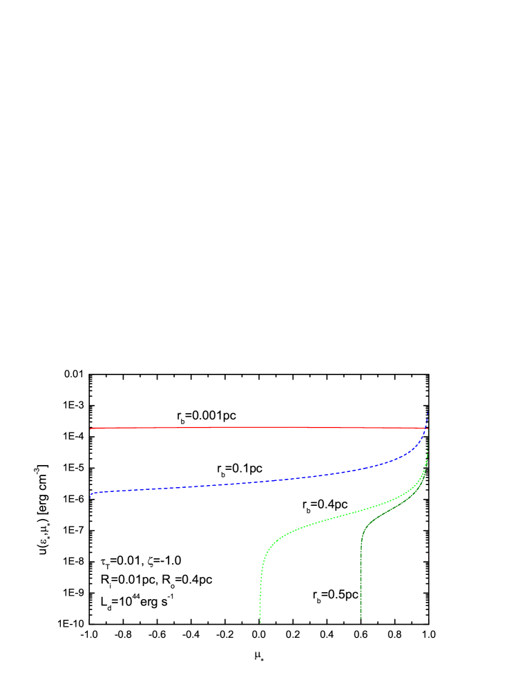
Figure 1: Angle-dependent energy density of BLR-scattered photon field. The values of $r_{\rm b}$ are labeled on the curves. The dimensionless photon energy is $\epsilon_{\ast}=2.48\times 10^{-5}$.

The intrinsic high energy photons flux from extragalactic sources is

$$f_{\rm intrinsic}(E_{\gamma})=e^{\tau(E_{\gamma},z)}f_{\rm observed}(E_{\gamma})\,,$$ (5)

where $f_{\rm observed}$ is the measured TeV flux, and $\tau(E_{\gamma},z)$ is the optical depth of $\gamma$-ray with energy $E_{\gamma}$ at redshift $z$. Here, we use the EBL model of Franceschini et al. (2008) to de-absorb the observed TeV spectra. This model is based on observations and takes into account all available information on cosmic sources contributing background photons.

Several parameters in our model can be constrained by observations. Böttcher et al. (2009) excluded extreme values of the Doppler factor in the range $\delta_{\rm D}\geq 50$. The size of the emission blob can be constrained by the observed variability timescales $t_{\rm var}$, because $R^{\prime}_{\rm b}=t_{\rm v,min}\delta_{D}c/(1+z)\leq\delta_{D}ct_{\rm tar}/(1+z)$. Here $R^{\prime}_{\rm b}$ is the radius of the blob in the co-moving frame, and $t_{\rm v,min}$ is the smallest variability timescale. Takalo et al. (1996) reported a micro-variability with $t_{\rm var}\sim 2.16\times 10^{4}$s and $\bigtriangleup\rm mag\sim 0.2$. Abdo et al. (2011) reported shorter variability at optical band: $t_{\rm var}\sim 1.44\times 10^{4}$s.

3 The results

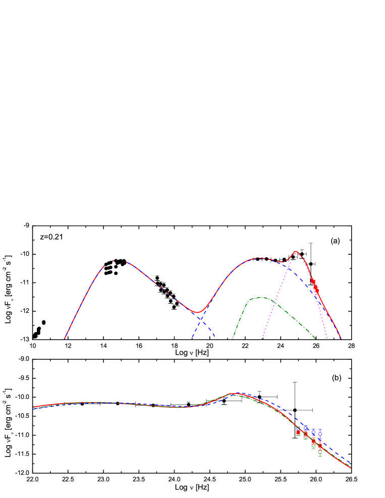
Figure 2: In panel (a), we show the reproduced SED with $z=0.21$. The filled square are the de-absorbed TeV data with $z=0.21$. The dashed, dash-doted, dotted and thick solid lines are SSC component, accretion-disk, BLR-reproduced component and the sum of multi-component, respectively. In panel (b), the open square, filled square and open circle are the de-absorbed TeV data with $z=0.15$, 0.21 and 0.31, respectively. The dash-dotted, solid and dashed lines are the model results at $z=0.15$, 0.21 and 0.31, respectively. All observed data are from Abdo et al. (2010b). See detailed data information in Abdo et al. (2010b).

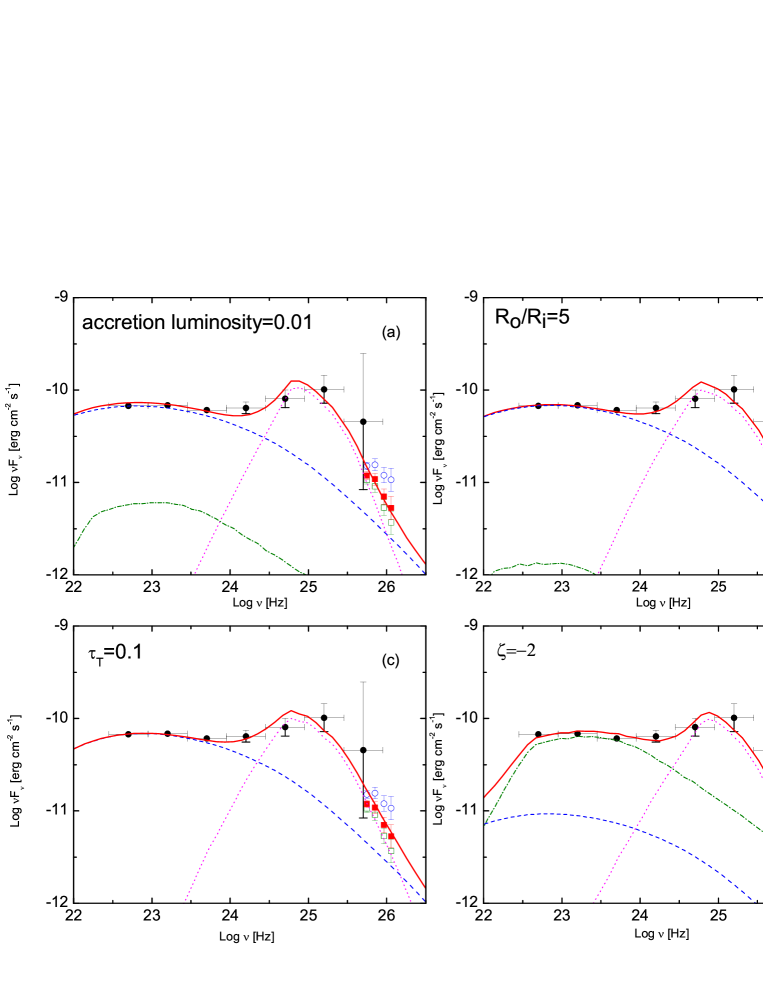
Figure 3: The effects of different assumptions of BLR structure and the characteristics of central source on the estimation of the redshift. The symbols are the same as that in Fig.  2.

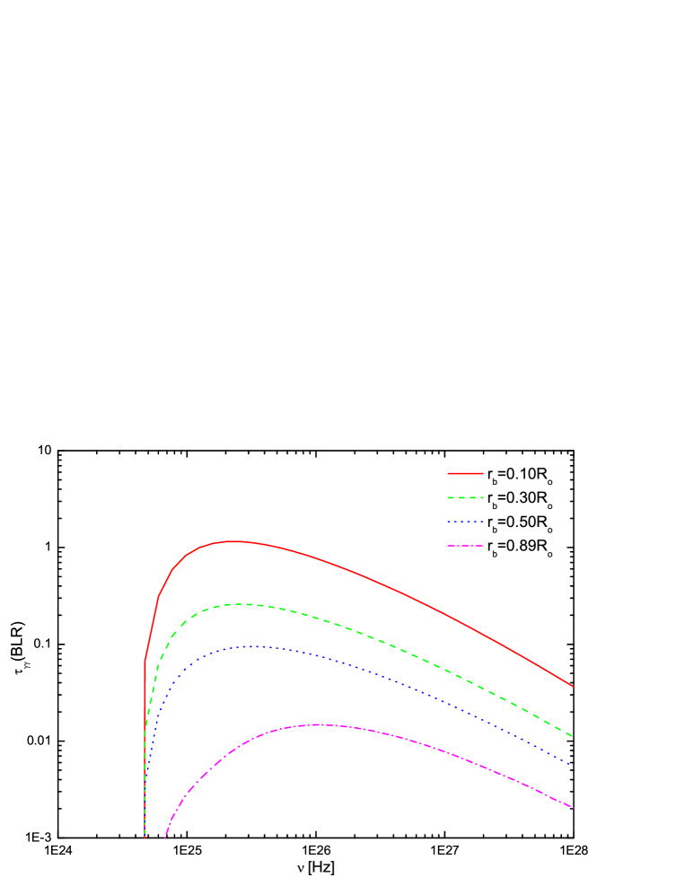
Figure 4: $\gamma\gamma$ optical depth for $\gamma$-ray interaction with BLR-reproduced photons at different distances from central BH when $z=0.21$.

Table 1: Model parameters for Fig. 2.

parameters	$z=0.15$	$z=0.21$	$z=0.31$
B (G)	0.168	0.168	0.168
$K^{\prime}_{\rm e}$ ($10^{53}$)	0.62	1.5	1.5
$p_{1}$	2.0	2.0	2.0
$p_{2}$	4.0	4.0	4.0
$\gamma_{\rm max}^{\prime}$($10^{6}$)	3.0	3.0	3.0
$\gamma_{\rm b}^{\prime}$($10^{3}$)	5.8	6.3	7.6
$\gamma_{\rm min}^{\prime}$($10^{3}$)	1.93	1.90	1.76
$\delta_{D}$	38	36	43
$t_{\rm v,min}$($10^{4}$s)	0.69	1.17	1.21
$M_{\rm 8}$	4.0	4.0	4.0
$\ell_{\rm Edd}$	0.03	0.03	0.03
$\eta$	0.1	0.1	0.1
$\tau_{\rm T}$	0.01	0.01	0.01
$\zeta$	-1.0	-1.0	-1.0
$R_{\rm i}$ ($10^{-2}$pc)	0.25	0.35	0.55
$R_{\rm o}$ (pc)	0.1	0.14	0.22
$r_{\rm b}$ ($R_{\rm o}$)	1.03	0.89	0.72

Table 2: Model parameters for Fig. 3.

parameters	$\ell_{\rm Edd}=0.01$	$\frac{R_{\rm o}}{R_{\i}}=5$	$\tau_{T}=0.1$	$\zeta=-2$
B (G)	0.168	0.168	0.168	0.168
$K^{\prime}_{\rm e}$ ($10^{53}$)	1.5	1.5	1.6	1.5
$p_{1}$	2.0	2.0	2.0	2.0
$p_{2}$	4.0	4.0	4.0	4.0
$\gamma_{\rm max}^{\prime}$($10^{6}$)	3.0	3.0	3.0	3.0
$\gamma_{\rm b}^{\prime}$($10^{3}$)	6.3	6.3	5.6	6.3
$\gamma_{\rm min}^{\prime}$($10^{3}$)	1.8	2.0	2.5	1.9
$\delta_{D}$	36	36	37	36
$t_{\rm v,min}$($10^{4}$s)	1.2	1.17	1.05	3.2
$M_{\rm 8}$	4.0	4.0	4.0	4.0
$\ell_{\rm Edd}$		0.03	0.03	0.03
$\eta$	0.1	0.1	0.1	0.1
$\tau_{\rm T}$	0.01	0.01		0.01
$\zeta$	-1.0	-1.0	-1.0
$R_{\rm i}$ ($10^{-2}$pc)	0.35	2.8	0.35	0.35
$R_{\rm o}$ (pc)	0.14	0.14	0.14	0.14
$r_{\rm b}$ ($R_{\rm o}$)	0.65	1.02	1.31	0.52

In Fig. 2, we show the modeling results at three different redshifts. The filled circles are quasi-simultaneous data from radio to GeV. The observed VERITAS data are EBL-corrected by using the EBL model of Franceschini et al. (2008) with different redshifts. It can be seen that the accretion-disk component is negligible compared to the SSC and BLR components. SSC and EC are responsible for emissions at the GeV-TeV bands. Emission between 0.1 GeV and 10 GeV is dominated by SSC. Above 10 GeV, the EC component of BLR is more important. Table 1 lists all model parameters.

It is interesting that the Klein-Nishina (KN) effect becomes important in Compton scattering the BLR radiation when $\gamma^{\prime}\Gamma_{\rm bulk}\epsilon_{\ast}\geq 1/4$, where $\Gamma_{\rm bulk}$ is the bulk Lorentz factor of the blob. In our model, $\Gamma_{\rm bulk}\approx\delta_{\rm D}$, so that $\gamma^{\prime}_{\rm KN}=280$. Electrons with this energy scatter photons primarily to energies of $\epsilon_{\rm KN}\approx\Gamma_{\rm bulk}\delta_{\rm D}\epsilon_{\ast}\gamma^{\prime 2}_{\rm KN}/(1+z)\approx 2.08\times 10^{3}$, which corresponds to frequency of $\nu_{\rm KN}\approx 2.57\times 10^{23}$Hz. Due to the KN effect, the BLR-component spectra at the right side of peak decline more quickly. In addition to large $\gamma_{\rm min}^{\prime}$, the KN effect is the other cause of the narrow BLR-component SED.

As shown in panel (b) of Fig. 2, the EBL-corrected TeV spectrum is steeper than the extrapolated one if the redshift is below 0.15. On the other hand, if the redshift is above 0.31, the EBL-corrected TeV spectra becomes harder. The EBL-corrected TeV emission can be well reproduced when z=0.21. Hence, the redshift of 3C 66A should be between 0.15 and 0.31, and the most likely redshift is 0.21. There are several poorly constrained parameters in our model. It should be discussed whether the uncertainties of model parameters can affect our results. As mentioned above, the contribution of the BLR component is dominant at TeV band, which is crucial for constraining the redshift of 3C 66A. The BLR structure ($R_{\rm i}$, $R_{\rm o}$, $\zeta$, $\tau_{\rm T}$) and the characteristics of the central source (the black hole and its accretion disk) can affect the contribution of the BLR component. $R_{\rm o}$ can be constrained by Eq.(2). We assumed typical values: $(\ell_{\rm Edd},R_{\rm o}/R_{\rm i},\tau_{\rm T},\zeta)=(0.03,40,0.01,-1)$, to reproduce the SED of 3C 66A. The effects of these parameters on estimating of the redshift are discussed by using other plausible boundary values. Results are shown in Fig. 3 (a), (b), (c) and (d). Parameters are listed in Table 2. For clarity, only the modeling results in the high energy part of the case $z=0.21$ are shown. Obviously, the SED (including TeV spectra) can also be reproduced well. We therefore argue that our results are independent of these parameters.

In addition, our results indicate that the gamma-ray emission region is beyond the inner zone of BLR ($\sim$0.1 pc, see Table 1 2). In Fig. 4, we show the $\gamma\gamma$ absorption by BLR-scattered radiation at different blob locations when taking $z=0.21$. There is a significant absorption when the blob is inside the inner zone of the BLR. Beyond the inner zone, absorption is negligible. No absorption feature at GeV band confirms that the emission region of 3C 66A should be out of the inner zone of BLR.

4 Discussion and conclusion

A pure SSC model fails to explain the average GeV spectrum of 3C 66A observed by Fermi-LAT during its first three months operation. While, a satisfactory reproduction of the data can be obtained by the multi-component model (see Fig. 2 3), which takes into account not only the specific shell structure of the BLR, but also the angular dependence of the photon distribution. The multi-component model requires a large value of $\gamma_{\rm min}^{\prime}\sim 2\times 10^{3}$. As argued by Tavecchio et al. (2009), this result seems to provide important clues to the electron acceleration process and the role of energy loss. A large value of $\gamma_{\rm min}^{\prime}$ leads to a steep spectrum in the low-energy band, so our model does not explain the observed radio emission. The radio emission may come from a larger emission region.

Based on the modeling results, we try to constrain the redshift of 3C 66A through connecting the GeV-TeV spectra. Because we can not give the error estimate by using this method, we think only the redshift range we derived is significant. It’s therefore suggested that the redshift of 3C 66A may be between 0.1 and 0.3, and the most likely one is $\sim$ 0.2. Furthermore, we found the results are independent of the assumptions about the BLR structure we made. By using different emission model and GeV-TeV data, we obtained the very similar results with that obtained by Abdo et al. (2011). However, it should be kept in mind that both our results and that of Abdo et al. (2011) depend on the EBL model. We also try to get clues on the gamma-ray emission location of 3C 66A. Combining the BLR absorption effect and the EC component required to reproduce the gamma-ray emission, our results indicate that the gamma-ray emission region of 3C 66A may be in the outer zone of BLR or out of BLR.