SUNGLASS: A new weak lensing simulation pipeline

Abstract

A new cosmic shear analysis pipeline SUNGLASS (Simulated UNiverses for Gravitational Lensing Analysis and Shear Surveys) is introduced. SUNGLASS is a pipeline that rapidly generates simulated universes for weak lensing and cosmic shear analysis. The pipeline forms suites of cosmological N-body simulations and performs tomographic cosmic shear analysis using line-of-sight integration through these simulations while saving the particle lightcone information. Galaxy shear and convergence catalogues with realistic 3D galaxy redshift distributions are produced for the purposes of testing weak lensing analysis techniques and generating covariance matrices for data analysis and cosmological parameter estimation. We present a suite of fast medium resolution simulations with shear and convergence maps for a generic 100 square degree survey out to a redshift of $z=1.5$, with angular power spectra agreeing with the theory to better than a few percent accuracy up to $\ell=10^{3}$ for all source redshifts up to $z=1.5$ and wavenumbers up to $\ell=2000$ for the source redshifts $z\geq 1.1$. At higher wavenumbers, there is a failure of the theoretical lensing power spectrum reflecting the known discrepancy of the Smith et al. (2003) fitting formula at high physical wavenumbers. A two-parameter Gaussian likelihood analysis of $\sigma_{8}$ and $\Omega_{m}$ is also performed on the suite of simulations, demonstrating that the cosmological parameters are recovered from the simulations and the covariance matrices are stable for data analysis. We find no significant bias in the parameter estimation at the level of $\sim 0.02$. The SUNGLASS pipeline should be an invaluable tool in weak lensing analysis.

1 Introduction

Cosmic shear analysis is an excellent method for probing the dark Universe (for reviews, see Mellier, 1999; Bartelmann & Schneider, 2001; Refregier, 2003; Schneider, 2006; Munshi et al., 2008; Massey et al., 2010, and references therein). It is also a reasonably new field of research with cosmic shear first being observed just ten years ago (Bacon et al., 2000; Kaiser et al., 2000; Van Waerbeke et al., 2000; Wittman et al., 2000). Weak gravitational lensing effects on a cosmic scale are a mere 1% change in shape and observational systematics makes the measurement of these changes challenging. However, the combination of the well-understood underlying physics and the expected precision of cosmological parameter estimation make the effort worthwhile.

Next generation telescope surveys will observe more of the sky than ever before and the volume of data they will produce is unprecedented. Future surveys promise to determine the equation of state of dark energy to 1% as well as probing the possibilities of extra dimensional gravity models and alternative cosmologies. The first Pan-STARRS telescope is currently undertaking a cosmic shear survey of the entire visible sky from its location in Hawaii and new projects such as VST-KIDS, DES, HALO, Euclid and LSST and are planned to perform wide field cosmic shear surveys, measuring both large, linear scales, and small, non-linear scales.

Due to the relative youth of this field, techniques are still being developed to exploit the weak lensing data from these surveys to provide further understanding on the nature of the Universe. To realise the potential of these new telescope surveys and to test new weak lensing analysis techniques, challenges must be met. To achieve the small statistical errors required, experiments require full end-to-end simulations of huge volumes which also probe the non-linear regime to assist in understanding the limitations of the analysis techniques. Simulations offer data sets with known parameters which are essential when testing analysis pipelines. Simulations can also include effects which may be difficult to model theoretically, such as source clustering and galaxy alignments, as well as other systematics and real-world effects. An additional role for simulations is in accurate estimation of the covariance of observable quantities. This is needed for the analysis of surveys and analytic approximations can be wholly inadequate (e.g. Semboloni et al., 2007). Monte Carlo analysis can be performed with simulations to provide covariance matrices that are required for data analysis and cosmological parameter estimation. Simulations are also required for rigorous testing and development so all analysis methods can be analysed blindly before the same techniques are applied to real data. To address these challenges, the SUNGLASS, Simulated UNiverses for Gravitational Lensing Analysis and Shear Surveys, pipeline has been developed to produce simulations and mock shear and convergence catalogues rapidly for weak lensing and cosmic shear analysis. The purpose of this paper is to introduce SUNGLASS and show rigorous testing of its outputs.

Many weak lensing studies use simulations with very high resolution to run their analysis (e.g. Fosalba et al., 2008; Hilbert et al., 2009; Teyssier et al., 2009; Schrabback et al., 2010). The computational cost of running these simulations is high and consequently there is often only a single realisation available. However, it is very important to ensure that covariance matrices calculated from these simulations are not contaminated by correlations in the simulations (Hartlap et al., 2007). In order to ensure uncorrelated data, a Monte Carlo suite of simulations should be used to determine the covariance matrix (Sato et al., 2009). In this work, 100 independent simulations were constructed using SUNGLASS.

To date, there are still reasonably few weak lensing simulations available. Of the few that are available, many implement a ray-tracing technique where light rays are propagated from an observer to a lensing source plane (e.g. Jain et al., 2000; Vale & White, 2003; Hilbert et al., 2009; Teyssier et al., 2009; Sato et al., 2009; Dietrich & Hartlap, 2010; Vafaei et al., 2010). Ray-tracing is computationally intensive and time consuming when solving the full ray-tracing equations. If the Born approximation is used in the ray-tracing, the time to run the analysis is reduced but the process is still computationally intensive and the simulation data still needs to be binned in three dimensions to perform the calculations. An alternative to ray-tracing is line-of-sight integration, which uses the Born approximation to calculate rapidly the weak lensing signal through a lightcone (e.g. White & Hu, 2000; Fosalba et al., 2008). This method is not suitable in the strong lensing regime but in the weak lensing regime, it is rapid and requires fewer computational resources than ray-tracing techniques. In this paper, a new line-of-sight integration technique, implemented in the SUNGLASS pipeline, for measuring convergences in an N-body simulation is introduced. This new method is rapid and can be run on a single processor of a desktop computer. In contrast to ray-tracing, the method does not bin in the radial direction, using all of the redshift information available. Although the catalogues are suitable for real-space analysis, SUNGLASS analyses and tests our mock weak lensing surveys in Fourier space, using power spectra, as it is possible to cleanly distinguish between linear and nonlinear regimes in Fourier space. We are also able to easily identify scales where the simulations are reliable by determining the region of the power spectrum in Fourier space that lies between the size of the simulated volume at low wavenumbers and shot-noise due to particle discreteness and pixelization effects at high wavenumbers.

The outline of this paper is as follows. Section 2 introduces the SUNGLASS pipeline. Details of the simulations are in section 2.1 and the line-of-sight integration method for determining shear and convergence without radial binning is described in section 2.2. Section 2.3 presents the shear and convergence power spectrum analysis and section 2.4 deals with the generation of the mock galaxy shear catalogues. An application of the mock catalogues is discussed in section 3 where Gaussian likelihood estimates of $\Omega_{m}$ and $\sigma_{8}$ are performed. A summary of the pipeline and methods concludes the paper in section 4.

2 Details of the SUNGLASS pipeline

SUNGLASS is a pipeline that generates cosmic shear and convergence catalogues using N-body simulations. The pipeline creates mock galaxy shear catalogues that can be used to test the cosmic shear analysis software used on telescope survey data sets. The nature of the pipeline also allows many simulation realisations to be generated rapidly to produce covariance matrices for data analysis and cosmological parameter estimation. The pipeline begins by creating a suite of cosmological N-body simulations. Lightcones are generated through the simulations and tomographic shear and convergence maps are determined using line-of-sight integrations at multiple lensing source redshifts. Finally, mock galaxy catalogues with fully 3D shear and convergence information and galaxy redshift distributions are assembled from the lightcones and the tomographic shear and convergence planes. The following sections detail each step of the SUNGLASS pipeline.

2.1 The N-body Simulations

All of the simulations presented in this work were run on a modest Xeon cluster, using 4 nodes with dual Xeon E5520 2.27 GHz quad-core processors per node and 24Gb shared memory per node. The simulations were run using the cosmological structure formation software package GADGET2 (Springel, 2005). GADGET2 represents bodies by a large number, N (in this work we use $512^{3}$), particles. Each particle is ‘tagged’ with its own unique kinematic and physical properties that evolve with the particle over time. GADGET2 models the dynamics of dark matter particles using a Tree-PM scheme and for the purposes of this work, only dark matter particles were considered.

The pre-initial particle distribution for the simulations used in this work is a glass which has sub-Poissonian noise properties (White, 1994). This distribution has no preferred direction with forces on each particle being close to zero. If a glass is used as the initial condition in a standard integrator, structures do not evolve. Particle displacements are imposed manually as an initial step to enable structure formation. The initial power spectrum was imposed on the particles using the parallel initial conditions generator N-GenIC that was provided by Volker Springel. The initial particle displacement field is formed by using the Zel’dovich approximation (Zel’dovich, 1970) to perturb the particles, imposing an Eisenstein & Hu (1998) matter power spectrum on the particles, and giving each particle an initial velocity.

Multiple medium-resolution simulations were run with $512^{3}$ dark-matter particles, in a box of $L=512h^{-1}$ Mpc comoving side length with periodic boundary conditions. The following cosmological parameters were used for a flat concordance $\Lambda$CDM model consistent with the WMAP 7-year results (Jarosik et al., 2010): $\Omega_{\Lambda}=0.73$, $\Omega_{m}=0.27$, $\Omega_{b}=0.045$, $n_{s}=0.96$, $\sigma_{8}=0.8$ and $h=0.71$ in units of 100 km  s^-1  Mpc^-1. The particle mass is $7.5\times 10^{10}$${\rm M}_{\odot}$and the softening length is $33h^{-1}$ kpc. The simulations were all started from a redshift of $z=60$ and allowed to evolve to the present.

The simulation data were stored at 26 output times corresponding to a $128h^{-1}$ Mpc comoving separation, between $z=1.5$ and the present. These snapshots were chosen to fall within the photometric redshift error of $\sigma_{z}<0.05(1+z)$ corresponding to a displacement of $\simeq 147h^{-1}$ Mpc at $z=1$. In a $512^{3}$ particle simulation, this amounts to 100GB data per simulation and takes approximately 21hrs to run on the Xeon cluster’s 32 processors.

2.2 Shear and Convergence Map Generation

We begin by determining the shear and convergence for a source plane at fixed comoving distance $r_{s}$. We consider a distribution of sources in Section 2.4.

The effects of weak gravitational lensing on a source can be described by two fields, the spin-2 shear, $\gamma$, which describes the stretching or compression of an image, and a scalar convergence, $\kappa$, which describes its change in angular size. These can be related to a lensing potential field, $\phi$, by

$$\kappa = \frac{1}{2}\partial^{2}\phi,$$ (1)

$$\gamma = \gamma_{1}+i\gamma_{2}=\frac{1}{2}\partial\partial\phi,$$ (2)

where $\gamma_{1}$ and $\gamma_{2}$ are the orthogonal components of the shear distortion, and $\partial=\partial_{x}+i\partial_{y}$ is a complex derivative on the sky.

We want to generate shear and convergence maps along a lightcone through the simulation. Instead of using ray tracing to determine the lightcone (e.g. Wambsganss et al., 1998; Jain et al., 2000; Teyssier et al., 2009; Hilbert et al., 2009), a line-of-sight integration was implemented using the Born approximation where one integrates along an unperturbed path (e.g. Cooray & Hu, 2002; Vale & White, 2003). Fosalba et al. (2008) build their convergence maps by adding slices from their simulation with the appropriate lensing weight and averaging over a pixel;

$$\bar{\kappa}(\mbox{\boldmath$\theta$}_{i},r_{s}) = \int_{0}^{r_{s}}dr~{}K(r,r_{s})~{}\bar{\delta}(\mbox{\boldmath$\theta$}_{i},r)$$ (3)

$$= \frac{3H_{0}^{2}\Omega_{m}}{2c^{2}}\sum_{j}~{}\bar{\delta}(\mbox{\boldmath$\theta$}_{i},r_{j})~{}\frac{(r_{s}-r_{j})r_{j}}{r_{s}a_{j}}~{}\Delta r_{j},$$ (4)

where $\mathbf{\theta}_{i}$ is the position if the $i^{th}$ pixel on the sky and $j$ is a bin in the radial direction which is at a distance of $r_{j}$ and has a width of $\Delta r_{j}$. An overline denotes an average over a pixel on the sky. The expansion factor at each radial bin $j$ is given by $a_{j}$ and the comoving radial distance of the lensing source plane is given by $r_{s}$. In order to make these calculations, the 3D matter overdensity $\bar{\delta}(\mbox{\boldmath$\theta$},r)$ must be calculated by binning the simulation data in three dimensions.

A limitation of this approach is memory, speed and accuracy. Here we propose, in the SUNGLASS pipeline, a new method for the line-of-sight integration so that no radial binning is required to determine the convergence. The particles are binned in a fine angular grid while allowing them to keep their radial co-ordinate.

Rewriting equation (4) we find the average convergence in an angular pixel, with no radial binning, is given by

$$\bar{\kappa}_{p}(r_{s})=\sum_{j}\frac{K(r_{j},r_{s})}{\Delta\Omega_{p}\bar{n}(r_{j})r_{j}^{2}}-\int_{0}^{r_{s}}\!dr~{}K(r,r_{s}),$$ (5)

where $\Delta\Omega_{p}=\Delta\theta_{x}\Delta\theta_{y}$ is the pixel area and $K(r,r_{s})$ is the scaled lensing kernel:

$$K(r,r_{s})=\frac{3H_{0}^{2}\Omega_{m}}{2c^{2}}\frac{(r_{s}-r)r}{r_{s}a(r)}.$$ (6)

Hereafter we drop the overline and assume all fields are averaged over an angular pixel. A derivation of equation (5) is given in Appendix A. In practice equation (5) can be calculated by a running summation so that it is not necessary to re-calculate the convergence from scratch for each source redshift.

Figure 1: Lightcone geometry through a simulation box volume. The lightcone travels through the first $128h^{-1}~{}$Mpc of the first simulation and then the next $128h^{-1}~{}$Mpc of the next simulation etc. At the end of the simulation volume, the next volume snapshots have their centroids shifted and are randomly rotated to avoid repeated structures along the lightcone.

The convergence maps are generated by adding the particles that fall within the lightcone to the line-of-sight integration. To show evolution through the lightcone, the simulation volumes are split into 128$h^{-1}$ Mpc sections. The first 128$h^{-1}$ Mpc of the first ($z=0$) snapshot is used, the second 128$h^{-1}$ Mpc of the second ($z>0$) snapshot and so on until the end of the simulation box volume is reached at snapshot 4 as shown in Figure 1. The centroid of the next simulation box is then shifted and the simulation box is rotated randomly to try to avoid repeated structures along the line-of-sight (e.g. White & Hu, 2000; Vale & White, 2003). The boxes are always periodic in the transverse direction. This continues through all of the snapshots out to a redshift of $z=1.5$. The source redshifts have been placed at $\Delta z=0.1$ intervals because the change in convergence between these redshifts is small enough that desired redshift values in between can be accurately determined by interpolation.

Once the convergences have been calculated at each of the source redshifts, the shear values can be determined on a flat-sky. The flat-sky shear and convergence Fourier coefficients are related by

$$\gamma_{1}(\boldsymbol{\ell}) = \kappa(\boldsymbol{\ell})\frac{(\ell_{x}^{2}-\ell_{y}^{2})}{(\ell_{x}^{2}+\ell_{y}^{2})},$$ (7)

$$\gamma_{2}(\boldsymbol{\ell}) = \kappa(\boldsymbol{\ell})\frac{2\ell_{x}\ell_{y}}{l_{x}^{2}+l_{y}^{2}},$$ (8)

where $\kappa(\boldsymbol{\ell})$ is the Fourier transform of the convergence and $\ell_{x}$ and $\ell_{y}$ are the Fourier variables. The Fast Fourier transform used throughout this paper is FFTW. The periodic nature of FFTW requires that the field is buffered with a small number of bins that are trimmed off after the shear has been calculated. To test the algorithm we also estimated B-modes by calculating the unphysical imaginary part of the convergence $\beta=\mathrm{imag}(\kappa)$, from the shear,

$$\beta(\mbox{\boldmath$\ell$})=\gamma_{1}(\mbox{\boldmath$\ell$})\left(\frac{2\ell_{x}\ell_{y}}{l_{x}^{2}+l_{y}^{2}}\right)+\gamma_{2}(\mbox{\boldmath$\ell$})\left(\frac{\ell_{x}^{2}-\ell_{y}^{2}}{\ell_{x}^{2}+\ell_{y}^{2}}\right).$$ (9)

Figure 2: Convergence and shear map for a simulated survey of 100 square degrees with a single source redshift of $z=0.8$. The colour-scale background shows the convergence while the white ticks show the shear signal.

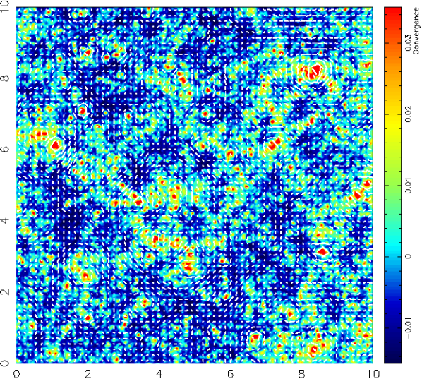
Figure 2 is an example of a convergence and shear map for a field that is 100 square degrees at a source redshift of $z=0.8$. There are 2048 bins in each transverse direction and no binning in the radial direction. The background of the map shows the integrated convergence along the lightcone up to $z=0.8$ and the white ticks show the shear at this source redshift. The length of the ticks has been multiplied by an arbitrary constant to make them visible as the magnitude of the shear is at the percent level. The red patches show areas of the highest convergence and the shear ticks clearly trace these regions tangentially. These maps can be generated for the standard simulations at multiple source redshifts quite rapidly once the simulations have been run. The most time consuming module in this code is reading in the snapshots due to their reasonably large size of 100GB. This module can be optimised by using the fastest available data transfer rates on the drive where the snapshot data is stored.

2.3 Shear and Convergence Power Spectra

Figure 3: Simulated slices of the shear power spectra for N-body particle data at source redshifts of $z=0.3$, $0.6$, $0.8$, $1.0$, $1.3$ and $1.5$. The smooth (red) line shows the theoretical predictions, the straight diagonal (blue) line is the predicted shot-noise at each source redshift. The black points are the mean power spectrum of the simulated data for the 100 realisations with errors on the mean shown and the (light blue) curve under these points is the simulation data with the shot-noise subtracted. The sub-shot-noise (magenta) curve is the estimated induced B-mode. The lower panel shows the fractional percentage difference between the simulated shear power and the theoretical prediction with black points representing the simulated data and light blue points representing the shot-noise subtracted simulation data.

In order to verify the accuracy of the shear and convergence maps, the shear and convergence power spectra are determined for each source redshift. From equation (4), the theoretical prediction for the shear and convergence power spectrum for sources at redshift $z$ is given by

$$C_{\ell}^{\gamma\gamma}(z)=C_{\ell}^{\kappa\kappa}(z)=\frac{9H_{0}^{4}\Omega_{m}^{2}}{4c^{4}}\int_{0}^{r_{s}}\!dr\,P\left(\frac{\ell}{r};r\right)\frac{[r_{s}(z)-r]^{2}}{r_{s}^{2}(z)a^{2}(r)},$$ (10)

(Munshi et al., 2008) where $P(\ell/r;r)$ is the 3D matter density power spectrum at a redshift $z$.

From the simulations it is possible to determine an angle-averaged power spectrum from the convergence and shear calculated in the lightcones. When taking in to consideration the conventions used in FFTW, the discretised convergence power spectrum for a slice in redshift is given as the sum over logarithmic shells in $\ell$-space as

$$\frac{\ell(\ell+1)\hat{C}_{\ell}^{\kappa\kappa}(z)}{2\pi}=\sum_{\ell{\rm\,in\,shell}}\frac{|\kappa(\mbox{\boldmath$\ell$},z)|^{2}}{n^{2}~{}\Delta\ln\ell},$$ (11)

where $n$ is the total number of bins in the Fourier transform and $\Delta\ln\ell$ represents the thickness of the shell in log $\ell$-space, and $\hat{C}_{\ell}^{\kappa\kappa}$ is the estimated power. Similarly the shear power is estimated by

$$\frac{\ell(\ell+1)\hat{C}_{\ell}^{\gamma\gamma}(z)}{2\pi}=\sum_{\ell{\rm\,in\,shell}}\frac{|\gamma_{1}(\mbox{\boldmath$\ell$},z)|^{2}+|\gamma_{2}(\mbox{\boldmath$\ell$},z)|^{2}}{n^{2}~{}\Delta\ln\ell}.$$ (12)

The B-mode power is estimated in the same way as the convergence.

The modes in this power spectrum are arranged on a square grid, which causes discreteness errors when binned in annuli at small $\ell$. To correct for this, the power is scaled by the ratio of the measured number of modes to the expected number of modes,

$$N_{exp}=g\pi(\ell_{max}^{2}-\ell_{min}^{2}),$$ (13)

where $g=(L/2\pi)^{2}$ is the density of states, $L$ is the size of the field in radians, $\ell_{max}$ and $\ell_{min}$ are the minimum and maximum wave numbers in this shell. The effect of this normalisation correction is about $10\%$ at the lower wave numbers while the higher wavenumbers remain largely unaffected. The discreteness correction is not perfect which is why the same slight zig-zag of the power spectrum is evident in all of the source redshift planes at wavenumbers $\ell<100$.

We can compare our simulated shear and convergence power spectra with the theoretical expectation. The theoretical power spectrum we use is determined using a code kindly provided by Benjamin Joachimi (as demonstrated in Joachimi & Schneider, 2008, 2009, 2010, and extensively tested against iCosmo(Refregier et al., 2008)). This code uses the method of Smith et al. (2003) for the non-linear power spectrum, the matter transfer function of Eisenstein & Hu (1998) and the analytical expression for the linear growth factor as given in Heath (1977).

Due to the discrete number of particles in an N-body simulation, the measured power spectrum measured will be the combined real shear and convergence power plus a shot-noise power contribution,

$$\hat{C}^{\kappa\kappa}_{\ell}=C^{\kappa\kappa}_{\ell}+C_{\ell}^{SN},$$ (14)

where $\hat{C}^{\kappa\kappa}_{\ell}$ is the power estimated from the simulation. The shot-noise power can be derived from equation (10) using a white-noise power spectrum, $P_{SN}(k,r)=1/\bar{n}_{3}(r)$, where $\bar{n}_{3}(r)$ is the 3-D mean comoving number density of particles in the simulation. The shot-noise power for the shear and convergence is then given by

$$C_{\ell}^{SN}=\frac{9H_{0}^{4}\Omega_{m}^{2}}{4c^{4}}\int_{0}^{r_{s}}\!dr\,\frac{(r_{s}-r)^{2}}{\bar{n}(r)r_{s}^{2}a(r)^{2}}.$$ (15)

Usually, for simulated particles, $\bar{n}$ will be a constant in comoving coordinates.

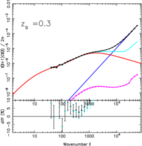
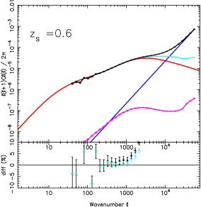
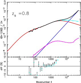
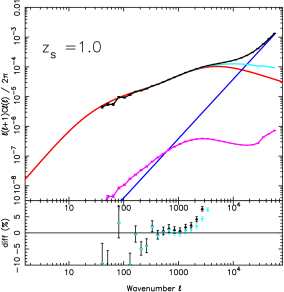
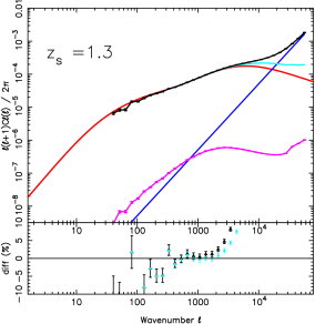
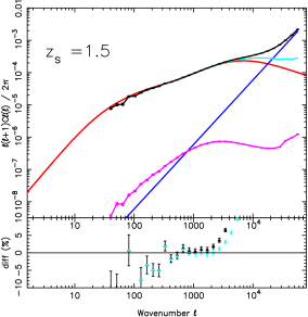
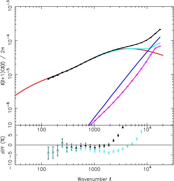
Figure 3 shows the mean, normalised 2-D shear power spectra estimated from 100 independent simulations (black points and line), with the error bars showing the scatter on the estimated mean. The figures show the shear power for sources at redshifts of $z=0.3,~{}0.6,~{}0.8,~{}1.0,~{}1.3~{}\textrm{and}~{}1.5$. The smooth (red) line shows the theoretical prediction for the ensemble-averaged shear power spectrum, while the diagonal (blue) lines show the shot-noise power for each source redshift. The (light blue) curve between the simulated data and the theory curve shows the mean power spectrum with the expected shot-noise subtracted and the lower (magenta) curve shows the estimated B-mode power spectrum.

The bottom panel of each figure shows the percentage difference between the measured shear power spectrum and the ensemble-average theory prediction (black), while the lower (light blue) points show the shot-noise subtracted shear power spectrum. Overall the mean shear power agrees well, to within a few percent, with the ensemble-averaged theoretical model over the $\ell$-range $\ell<1000$ for all source redshifts. The difference of a few percent is due to the fact that the theory 3D matter density power spectrum is a few percent lower than the measured data power spectrum. Calculating the highly non-linear power spectrum is currently not accurate to a few percent and many calculations of this theory curve do not agree with each other to within a few percent. The Joachimi theory curve was the closest fit to the simulations and was used for all subsequent calculations. At low $\ell$ the measured signal drops as we reach the size of the simulation box, while at high $\ell$, the estimated mean shear power becomes shot-noise dominated before reaching the highest mode allowed by the resolution of the angular pixels beyond $\ell=1/\theta_{\rm pix}\simeq 10^{4}$.

Before reaching pixel-resolution, the measured shear power at high-$\ell$ agrees well with the predicted shot-noise. This agreement suggests that the shot-noise model works well in this regime, even though the initial particle distribution is a glass (see Baugh et al., 1995, for a discussion). This suggests an improved estimate of the mean power can be found by subtracting off the shot-noise contribution. However, the shot-noise subtracted shear power does not follow the ensemble-averaged theoretical power estimated from the theory code. It is likely this is a failure of the theoretical model of lensing – on small-scales the Smith et al. (2003) nonlinear correction formula is known to underestimate the matter-density power spectrum, $P(k)$, by up to 10% at wavenumbers of $k<1$ and as great as 50% at $k=10$ Mpc^-1 (Giocoli, private communication) and hence has been shown to underestimate the shear and convergence power spectrum by up to 30% on scales of $\ell<10^{4}$ (Hilbert et al., 2009). In the absence of accurate fitting formulae, simulations like those presented in this paper may be used to improve theoretical predictions. However, this needs to be explored in more detail before it is fully understood so in subsequent analysis in this paper we will restrict our analysis to the region of the measured power spectrum that agrees with the theoretical prediction.

Figure 3 also shows the estimated B-mode power spectra. When galaxies trace the shear signal, we expect the B-mode power to pick up a shot-noise dependence. But here the shear signal is a pixelized field which would be continuous in the limit of infinite pixels. Therefore we do not expect there to be a noise-generated B-mode. However, B-modes can still be generated due to leakage of power from the convergence field caused by the finite window function when we generate the shear field from equation (8). As a consequence the induced B-mode has the shape of the shear power, but suppressed by around three orders of magnitude.

In this section we have shown that the SUNGLASS algorithm for calculating the shear and convergence maps and the power spectra in redshift slices is accurate to a few percent over a wide range of scales and redshifts. Wavenumbers up to $1500$ can be recovered for the source redshifts $z\geq 1.1$ with this simulation resolution. For shot-noise subtracted power spectra, the recovered modes increase before the angular pixel resolution cuts off the power.

2.4 Mock 3-D Weak Lensing Galaxy Catalogues

$N_{\rm Surveys}$	Area	$n$	$z_{\rm median}$	$\sigma_{0}$	$z_{\rm max}$
100	100	15	0.82	0.05	1.5

Table 1: Table of mock weak lensing survey parameters used in this paper.

Real, 3-D weak lensing data analysis is applied to a galaxy catalogue where galaxy angular positions and redshift are added to estimated shears for each galaxy. For a 2-D analysis, individual redshifts are ignored and the theory uses only the redshift distribution. It is straightforward to generate a simple 3-D mock weak lensing galaxy catalogue with the information in the lightcones we have generated from the simulations. Shear and convergence maps are generated for each lensing source redshift and then each particle in the simulation is assigned a shear and convergence by interpolating between adjacent planes. The error introduced by linearly interpolating the shear and convergence between source redshift planes separated by $\Delta z=0.1$ was estimated by comparing with much higher redshift-sampled planes and found to be substantially below the theoretical prediction ($\Delta C_{\ell}^{\gamma\gamma}<10^{-7}$) except at angular wavenumbers where shot-noise becomes dominant. With the interpolated shear and convergence assigned to each particle, we now have a fully-sampled 3-D mock weak lensing galaxy catalogue, which can be down-sampled to generate realistic weak lensing surveys.

Figure 4: Left: The galaxy distribution, $n(z)$, in the mock galaxy catalogue. The smooth (red) line shows the theoretical $n(z)$ and the black histogram shows the distribution from a single simulation lightcone. The histogram shows the clustered nature of the lightcone. Right: The galaxy distribution in the mock galaxy catalogue with photometric redshift errors assigned to each galaxy. The structures visible in the true redshift lightcone have been smoothed out with the addition of the photo-z errors.

To down-sample the full 3-D weak lensing simulated lightcone to construct a realistic 3-D weak lensing galaxy catalogue, we use a galaxy redshift distribution (Refregier et al., 2004)

$$n(z)\propto z^{\alpha}\exp\left[-\left(\frac{z}{z_{0}}\right)^{\beta}\right],$$ (16)

where $z_{0}$, $\alpha$ and $\beta$ set the depth, low-redshift slope and high-redshift cut-off for a given galaxy survey. We take $\alpha=2$, $\beta=2$ and $z_{0}=0.78$, yielding a median redshift of $z_{m}=0.82$, similar to the CFHTLens Survey.

As the particles in our simulation are in comoving coordinates, we transform this redshift distribution to a probability distribution for the particle to enter our catalogue given its comoving radial distance,

$$p(r)\propto r^{\alpha}\left(\frac{dr}{dz}\right)\exp\left[-\left(\frac{z(r)}{z_{0}}\right)^{\beta}\right],$$ (17)

where

$$\frac{dr}{dz}=\frac{c}{H(z)},$$ (18)

and

$$H(z)=\frac{H_{0}}{\left[\Omega_{m}(1+z)^{3}+\Omega_{K}(1+z)^{2}+\Omega_{\Lambda}\right]^{1/2}},$$ (19)

where $H_{0}$ is the current Hubble value, $\Omega_{m}$ is the current matter density, $\Omega_{\Lambda}$ is the current dark energy density and $\Omega_{K}$ is the curvature parameter. Throughout we have assumed a flat, $\Omega_{K}=0$, cosmology for our simulations. We sample the particle distribution so our final galaxy catalogue has a surface density of around 15 galaxies per square arcmin, with a maximum redshift cut-off at $z=1.5$.

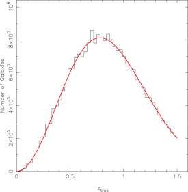
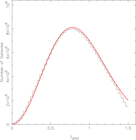
The left panel of Figure 4 is an example of a redshift distribution taken from the full particle lightcone. The red line shows the theoretical distribution from equation 17, normalised to the number of particles selected, that the simulation particles were drawn from. The clustered nature of the particles in the distribution is apparent as the peaks and troughs around the theoretical curve can be seen.

Figure 5: 2D shear power spectrum for the lightcone suite with the $n(z)$ particle distribution. In the upper panel, the smooth (red) line is the theory prediction and the diagonal (blue) line is the shot noise prediction. The (black) points and line is the mean measured power spectrum for the suite of mock catalogues with the errors representing the error on the mean and the curve between the theory prediction and the measured simulation data is the shot-noise subtracted power spectrum. The diagonal (magenta) line shows the mean of the B-modes for the suite of mock catalogues with errors on the mean. The bottom panel shows the percentage difference of the data from the theory curve with errors on the mean (black) and the lower (light blue) points represent the shot-noise subtracted data.

Our 3-D weak lensing catalogue currently assumes that the redshift to each galaxy is accurately known. This would be appropriate for a spectroscopic redshift survey, but with such large surveys we can expect most weak lensing catalogues will contain photometric redshift estimates for each galaxy. To account for photometric redshift errors, we randomly sample the measured redshift from the true redshift using a Gaussian distribution with uncertainty

$$\sigma_{z}=\sigma_{0}(z_{g})(1+z_{g}),$$ (20)

where $z_{g}$ is the true redshift of the particle. For the purposes of this work we assume a fixed $\sigma_{0}=0.05$. The right-hand panel of Figure 4 shows what the distribution on the left looks like with photometric redshift errors. The structures are smoothed out and the distribution becomes featureless. The photometric redshift errors were implemented by specifying a Gaussian error.

Figure 5 shows the ensemble-averaged 2-D shear power spectrum estimated from 100 mock weak lensing surveys in the top panel (black dots) with errors on the mean, compared the theoretical prediction in red, and the ensemble-averaged B-mode power in magenta. The (blue) diagonal line shows the shot-noise prediction for these galaxy redshift distributed lightcones. The shot-noise was determined by running the SUNGLASS analysis on a number of simulation box volumes filled with randomly distributed particles. The power spectrum of these lightcones represents shot-noise estimate for the simulations and is a remarkably straight power law. The (light blue) curve between the shot noise and the measured power spectrum is the shot-noise subtracted power spectrum. The bottom panel shows the fractional difference between the average of the mock surveys and the theory curve, with the error on the mean (black) and the shot-noise subtracted points below (light blue). This shows that the mock weak lensing survey agrees with the theoretical expectation from wavenumbers from $\ell=200$ to $\ell=2000$, where the disagreement with theory can be ascribed to the uncertainty on the theory curve, and the rise of shot-noise. The shot-noise subtraction in this case is a few percent lower than the theoretical prediction and the reason for this is not well understood and is the subject of ongoing investigation. The analyses in this paper will use the measured simulation power spectrum only. The B-mode power appears to follow a shot-noise profile which is consistent with the effect of sampling from the full particle lightcone. A secondary source for B-modes is source clustering, which appears to be sub-dominant.

We found a dependence for the recovered shear and convergence power on the number of pixels used to estimate the 2-D lensing power. With too many bins, there were a number of empty pixels and this reduced the amplitude of the power spectrum. The amplitude of the power spectrum increased with fewer empty bins before converging at the true amplitude. However, by using too few bins, the number of $\ell$ modes recovered was reduced due to pixelization effects. It was found that for this work, $768^{2}$ bins provided a stable amplitude for the power spectrum with the largest number of modes possible without causing this amplitude to fall. In this case, 0.03% of the bins are empty. If this number is increased to 5% empty, the amplitude of the power spectrum drops by up to 10%. This effect will also be important for observational studies and should be considered when binning survey data to determine 2D lensing power spectra.

3 Parameter Estimation

Figure 6: Histogram of the distribution of power spectra for the suite of lightcones with the $n(z)$ particle distribution. The left panel shows the distribution of the $C_{\ell}^{\gamma\gamma}s$ less than $\ell=400$, the middle panel shows the $C_{\ell}^{\gamma\gamma}$ distribution from $400<\ell<1300$ and the right panel shows the distribution from at $\ell>1300$.

As described in the previous Section 100 simulations have been generated using the SUNGLASS pipeline. The mock survey parameters are given in Table 1.

For each of these mock lensing surveys the shear and convergence power spectra has been estimated, and the ensemble average power and its scatter measured. Here we want to use the mock surveys to test a maximum likelihood cosmological parameter estimation analysis, typically used to extract parameters from weak lensing surveys. Here we try and recover the amplitude of the matter clustering, $\sigma_{8}$, and density parameter, $\Omega_{m}$, from a 2-D weak lensing survey.

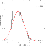
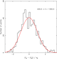
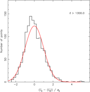
In Section 2.4 we showed that our simulations could produce unbiased estimates of the shear power from a mock survey over a range of $\ell$-modes from $200$ to $2000$. For parameter estimation we need to know the conditional probability distribution of shear power, $p(\hat{C}_{\ell}^{\gamma\gamma}|\sigma_{8},\Omega_{m})$, for the likelihood function, where we have fixed all other parameter at their fiducial values. This is usually assumed to be Gaussian (although, see Hartlap et al., 2009, who study non-Gaussian likelihoods). Here we test this assumption on our mock catalogues. Figure 6 shows the distribution of variations about the mean of the $\hat{C}_{\ell}$’s, $\Delta\hat{C}_{\ell}^{\gamma\gamma}$, divided by the ensemble-averaged scatter in the power, $\sigma(\hat{C}_{\ell}^{\gamma\gamma})$. If the distribution is Gaussian, these distributions should all lie on the unit-variance Gaussian. The left panel shows a histogram of the distribution of points for modes of $\ell<400$ which is close to the linear region of the power spectrum. The middle panel shows the distribution of $C_{\ell}^{\gamma\gamma}$ for modes of $400<\ell<1300$ which represents the non-linear region of the power spectrum. The final panel shows the distribution for modes $\ell>1300$ which is the shot-noise dominated regime. The smooth (red) line in each of the panels is a normalised unit-Gaussian curve. In each of the panels, the histogram of points is peaked slightly to the left of the Gaussian peak which indicates a slight non-Gaussianity of the distribution of points. This slight non-Gaussianity may bias the Gaussian likelihood analysis but the dominant effect is currently the inaccurate fitting of the matter power spectrum by the Smith et al. (2003) formula at high $k$ (Giocoli et al., 2010).

The cosmological parameters of the simulations were estimated using Gaussian likelihood analysis where the likelihood is given by

$$L(\hat{C}_{\ell}^{\gamma\gamma}|\sigma_{8},\Omega_{m})=\frac{1}{(2\pi)^{N/2}(\mathrm{det}~{}M_{\ell\ell^{\prime}})^{1/2}}\exp\left[\frac{-\chi^{2}}{2}\right],$$ (21)

where

$$\chi^{2}=\sum_{\ell\ell^{\prime}}(\hat{C}_{\ell}^{\gamma\gamma}-\langle C_{\ell}^{\gamma\gamma}\rangle)M_{\ell\ell^{\prime}}^{-1}(\hat{C}_{\ell^{\prime}}^{\gamma\gamma}-\langle C_{\ell^{\prime}}^{\gamma\gamma}\rangle),$$ (22)

and $M_{\ell\ell^{\prime}}$ is the covariance matrix of the shear power spectra given by

$$M_{\ell\ell^{\prime}}=\langle\Delta C_{\ell}^{\gamma\gamma}\Delta C_{\ell^{\prime}}^{\gamma\gamma}\rangle.$$ (23)

The inverse covariance matrix was determined by performing a singular value decomposition (SVD) on the covariance matrix (Press et al., 1992). The resulting inverse covariance matrix is, however, biased due to noise in the covariance matrix. Hartlap et al. (2007) propose a correction for this bias by multiplying the inverse covariance matrix by a factor:

$$\hat{M}^{-1}_{\ell\ell^{\prime}}=\frac{N_{S}-N_{p}-2}{N_{S}-1}M^{-1}_{\ell\ell^{\prime}},$$ (24)

where $N_{S}$ is the number of simulations used to determine the covariance matrix, $N_{p}$ is the number of bins in the power spectrum and $\hat{M}^{-1}_{\ell\ell^{\prime}}$ is the unbiased covariance matrix.

The likelihood analysis relies on accurate estimation of the covariance matrix to show the degree of correlations. The correlation coefficients are

$$r_{\ell\ell^{\prime}}=\frac{M_{\ell\ell^{\prime}}}{\sqrt{M_{\ell\ell}M_{\ell^{\prime}\ell^{\prime}}}}.$$ (25)

The correlation coefficient matrix is equal to 1 along the diagonal and the off diagonal components will show how correlated the $\ell$ modes are, with numbers close to zero indicating low correlation and numbers close to (minus) one indicating high (anti-)correlation.

Figure 7 shows the correlation coefficient matrix for the $\ell$ modes being considered between $100<\ell<2500$. The modes with a low correlation are represented in black and dark blues and the modes with a high correlation shown in yellows and reds. This shows the the bandpowers at low $\ell$ have very little correlation between them, as we would expect, since for an all-sky survey the linear power is uncorrelated. At higher $\ell$ bandpower, the modes become more correlated, due to cross-talk between different scales due to nonlinear clustering in the matter power spectrum. The variations in this coefficient matrix indicate an error of around 10% which is suitable for the studies in this paper. This error can be reduced by introducing more realisations into the calculations. In our analysis we shall consider modes up to $\ell=1500$, where the correlation coefficient is around $r_{\ell\ell^{\prime}}\approx 0.6$ .

Figure 7: Correlation coefficient matrix. This figure shows the correlation between the bandpower $\ell$-modes in the covariance matrix. The higher $\ell$ bandpowers are strongly correlated (shown in reds), while the lower bandpowers are only weakly correlated (shown in blues).

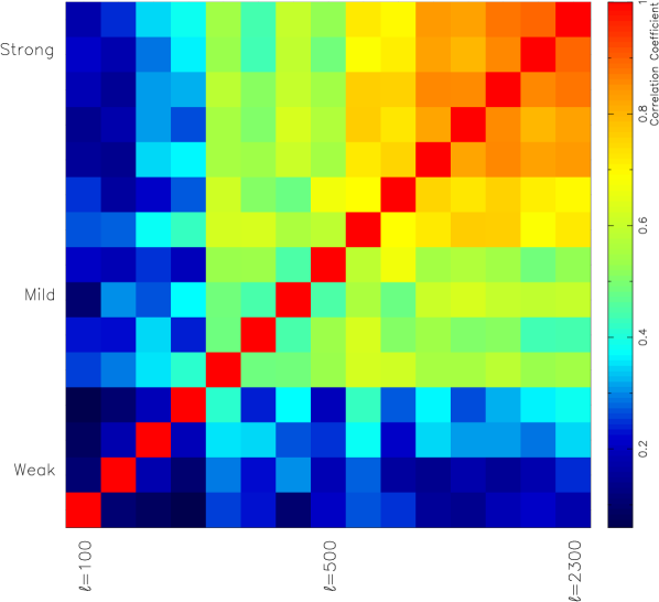
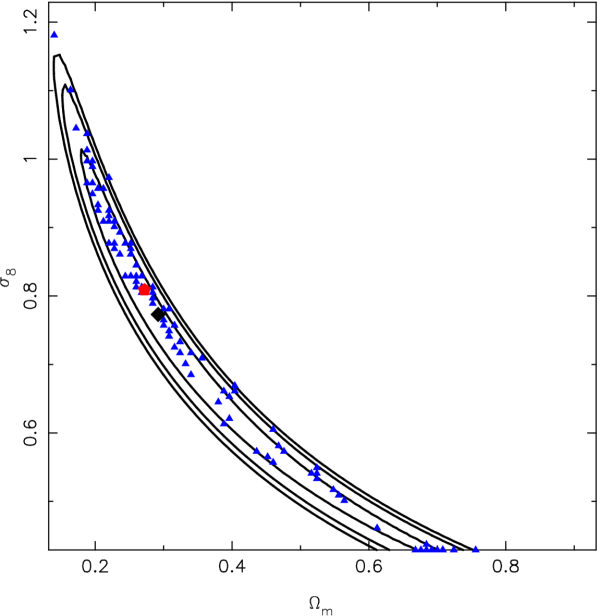
Figure 8 shows the $\chi^{2}$-distribution in the $\sigma_{8}$-$\Omega_{m}$ plane for our ensemble of simulations. The black lines represent the $\chi^{2}$ two-parameter, 1, 2 and 3$\sigma$ (which should contain 68.3%, 95.4% and 99.7% of the points assuming a bivariate Gaussian distribution), contours of parameter space for the cosmological parameters. However, this clearly is not a bivariate Gaussian distribution. The contours shown are representative and come from the simulation that had the best fit parameters that were closest to the true input parameters (the point shown by the red polygon). The blue triangles represent the best fit points for each of the 100 realisations. With this distribution, 68% of the points lie within the 1$\sigma$ contour, 93% within the 2$\sigma$ contour and 97% within the 3$\sigma$. The black diamond represents the best fit for the combined $\chi^{2}$ estimate as discussed below.

Figure 8: Gaussian likelihood estimate. The black contours come from the simulation with the closest fit to the true cosmological parameters. The blue triangles show the best fit cosmological parameters for the suite of lightcones. The true cosmological parameters are shown at the red polygon and the combined $\chi^{2}$ best fit parameter is shown at the black diamond.

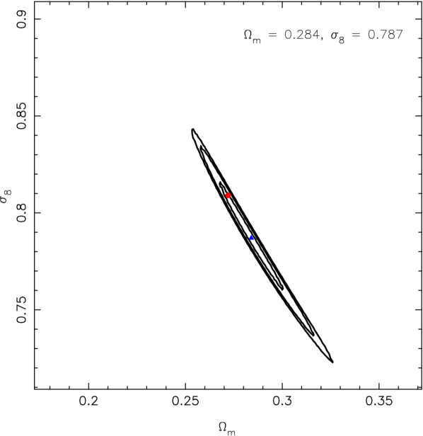
The results from this analysis give us very encouraging results for the parameter estimation. Figure 9 shows the results of combining the likelihoods for all 100 realisations, as if we have one hundred independent 100 square degree surveys. Even for this test we see the maximum likelihood recovered parameter values lie within the $1-\sigma$ confidence contour. The marginalised error on the measured parameters for the combined 100 surveys is $\Delta\Omega_{m}=0.012$ and $\Delta\sigma_{8}=0.022$, within expected errors. There is no significant bias in this result at the level of $\sim 0.02$.

Figure 9: Combined $\chi^{2}$ likelihood. The black lines show the combined $\chi^{2}$ 1, 2 and 3$\sigma$ contours. The blue triangle shows the best fit parameters for the combined $\chi^{2}$ and the red star shows the true cosmological parameters.

4 Discussion and Conclusions

This work introduces SUNGLASS – Simulated UNiverses for Gravitational Lensing Analysis and Shear Surveys. SUNGLASS is a new, rapid pipeline that generates cosmological N-body simulations with GADGET2. It computes weak lensing effects along a lightcone using line-of-sight integrations with no radial binning and the Born approximation to determine the convergence and shear at multiple source redshifts. This information is interpolated back on to the particles in the lightcone to generate mock shear catalogues in 3D for testing weak lensing observational analysis techniques.

In this work, SUNGLASS was used to generate 100 simulations with $512^{3}$ particles, a box length of $512h^{-1}$ Mpc and a WMAP7 concordance cosmology. The corresponding mock shear catalogues were 100 sq degrees with a source redshift distribution with median $z_{m}=0.82$ and 15 galaxies per square arcminute. The parameters are easily changed within the SUNGLASS pipeline so that the mock shear catalogues matches the survey of interest.

To show the reliability of the lightcones generated with SUNGLASS, E- and B-mode power spectra were shown at multiple source redshifts. The results show that at low redshifts, the signal becomes dominated by shot-noise at reasonably low $\ell$. With increasing source redshift, the power spectrum recovers the theoretical prediction over a wider range of modes, $\ell<2500$.

Given that the measured power spectrum of the simulations appears to follow the predicted shot noise at higher modes, the shot noise was subtracted from the power spectra to increase the recovered range. The theoretical prediction is expected to under predict the power spectrum around the turn over and consequently, the simulations could be recovering the power spectrum up to around $\ell=5\times 10^{4}$ at the highest redshift planes.

The multiple source redshift plane shear and convergence was interpolated onto the particles in the lightcone to generate a mock shear catalogue. A redshift sampling was also imposed on the lightcone to mimic an observed shear catalogue. Binning this distribution too finely resulted in empty bins which had the effect of suppressing the power spectrum. This has implications for observations where the number of objects per square arcminute should be taken into account, as well as the density of the binning, when determining the accuracy of the power spectrum.

The mock shear catalogues were used to determine a covariance matrix which is essential for both parameter estimation and data analysis. A strength of SUNGLASS is the ability to rapidly produce Monte Carlo realisations of these catalogues, ensuring independent mock data sets for the generation of the covariance matrices.

The mock catalogues were also used to perform a simple parameter estimation using Gaussian likelihood analysis. The distribution of power spectra were shown to be reasonably Gaussian and the resulting parameter estimation contours for a single realisation showed a good agreement with the input parameters within the 2-parameter 1,2 and 3$\sigma$ error contours.

The combined likelihood from the 100 simulations shows narrow likelihood contours and accurate parameter recovery within the expected errors, with no evidence of significant bias at the level of $\sim 0.02$.

Current and future telescope surveys promise to provide an enormous amount of data for weak lensing analysis. Weak lensing is still a young field and analysis techniques are still being developed. It is essential that the strengths and weaknesses of these techniques are fully understood before using them on real data with unknown parameters. Using the simulations, lightcones and mock shear catalogues provided by the SUNGLASS pipeline, and demonstrated in this paper, is an excellent way to test these observational weak lensing analysis techniques. The outputs of this pipeline have been rigorously tested and are well understood, making them ideal for generating covariance matrices that are critical to many observational analysis techniques.

Appendix A Derivation of the line-of-sight convergence with no radial binning

This appendix shows how the line-of-sight convergence shown in equation 5 was derived.

Start with the general equation for the convergence,

$$\kappa=\int_{0}^{r_{s}}dr~{}K(r,r_{s})~{}\delta(\mbox{\boldmath$r$}),$$ (26)

where $r_{s}$ is the lensing source redshift, $\delta(\mbox{\boldmath$r$})$ is the fractional matter overdensity and $K(r,r_{s})$ is the kernel

$$K(r,r_{s})=\frac{(r_{s}-r)r}{r_{s}a(r)}\frac{3H_{0}^{2}\Omega_{m}}{2c^{2}}.$$ (27)

The overdensity $\delta(\mbox{\boldmath$r$})$ is given by

$$\delta(\mbox{\boldmath$r$})=\frac{n(\mbox{\boldmath$r$})}{\bar{n}(r)}-1,$$ (28)

where $\bar{n}(r)$ is the average density at the comoving radial distance $r$ and is constant in comoving co-ordinates.

The particle number density, $n(\mbox{\boldmath$r$})$, is given by a sum of 3D delta functions

$$n(\mbox{\boldmath$r$})=\sum_{i=part}\delta^{3D}(\mbox{\boldmath$r$}-\mbox{\boldmath$r$}_{i})=\sum_{i}\frac{\delta^{1D}(r-r_{i})}{r^{2}}\delta^{2D}(\mbox{\boldmath$\theta$}-\mbox{\boldmath$\theta$}_{i}),$$ (29)

where $part$ are the particles in the pixel with $r_{i}\leq r_{s}$. Substituting this sum of delta-functions into equation (26) yields the average convergence per pixel on the sky, $p$, with no radial binning;

$$\bar{\kappa}_{p}=\frac{1}{\Delta\Omega}\int_{p}\!d^{2}\theta\,\kappa=\sum_{i}\frac{k(r_{i},r_{s})}{\Delta\Omega_{p}\bar{n}(r_{i})r_{i}^{2}}-\int_{0}^{r_{s}}dr~{}k(r,r_{s}),$$ (30)

where $\Delta\Omega_{p}=\Delta\theta_{x}\Delta\theta_{y}$.

References

- Bacon et al. (2000) Bacon D. J., Refregier A. R., Ellis R. S., 2000, MNRAS, 318, 625
- Bartelmann & Schneider (2001) Bartelmann M., Schneider P., 2001, Phys. Rep., 340, 291
- Baugh et al. (1995) Baugh C. M., Gaztanaga E., Efstathiou G., 1995, MNRAS, 274, 1049
- Cooray & Hu (2002) Cooray A., Hu W., 2002, ApJ, 574, 19
- Dietrich & Hartlap (2010) Dietrich J. P., Hartlap J., 2010, MNRAS, 402, 1049
- Eisenstein & Hu (1998) Eisenstein D. J., Hu W., 1998, ApJ, 496, 605
- Fosalba et al. (2008) Fosalba P., Gaztañaga E., Castander F. J., Manera M., 2008, MNRAS, 391, 435
- Giocoli et al. (2010) Giocoli C., Bartelmann M., Sheth R. K., Cacciato M., 2010, MNRAS, pp 1052–+
- Hartlap et al. (2009) Hartlap J., Schrabback T., Simon P., Schneider P., 2009, A&A, 504, 689
- Hartlap et al. (2007) Hartlap J., Simon P., Schneider P., 2007, A&A, 464, 399
- Heath (1977) Heath D. J., 1977, MNRAS, 179, 351
- Hilbert et al. (2009) Hilbert S., Hartlap J., White S. D. M., Schneider P., 2009, A&A, 499, 31
- Jain et al. (2000) Jain B., Seljak U., White S., 2000, ApJ, 530, 547
- Jarosik et al. (2010) Jarosik N., Bennett C. L., Dunkley J., et al. 2010, arXiv:astro-ph/1001.4744
- Joachimi & Schneider (2008) Joachimi B., Schneider P., 2008, A&A, 488, 829
- Joachimi & Schneider (2009) Joachimi B., Schneider P., 2009, A&A, 507, 105
- Joachimi & Schneider (2010) Joachimi B., Schneider P., 2010, A&A, 517, A4+
- Kaiser et al. (2000) Kaiser N., Wilson G., Luppino G. A., 2000, astro-ph/0003338
- Massey et al. (2010) Massey R., Kitching T., Richard J., 2010, Reports on Progress in Physics, 73, 086901
- Mellier (1999) Mellier Y., 1999, ARA&A, 37, 127
- Munshi et al. (2008) Munshi D., Valageas P., van Waerbeke L., Heavens A., 2008, Phys. Rep., 462, 67
- Press et al. (1992) Press W. H., Teukolsky S. A., Vetterling W. T., Flannery B. P., 1992, Numerical recipes in FORTRAN. The art of scientific computing
- Refregier (2003) Refregier A., 2003, ARA&A, 41, 645
- Refregier et al. (2008) Refregier A., Amara A., Kitching T., Rassat A., 2008, ArXiv e-prints
- Refregier et al. (2004) Refregier A., Massey R., Rhodes J., Ellis R., Albert J., Bacon D., Bernstein G., McKay T., Perlmutter S., 2004, AJ, 127, 3102
- Sato et al. (2009) Sato M., Hamana T., Takahashi R., Takada M., Yoshida N., Matsubara T., Sugiyama N., 2009, ApJ, 701, 945
- Schneider (2006) Schneider P., 2006, in Meylan G., Jetzer P., North P., Schneider P., Kochanek C. S., Wambsganss J., eds, Saas-Fee Advanced Course 33: Gravitational Lensing: Strong, Weak and Micro Part 3: Weak gravitational lensing. pp 269–451
- Schrabback et al. (2010) Schrabback T., Hartlap J., Joachimi B., et al. 2010, A&A, 516, A63+
- Semboloni et al. (2007) Semboloni E., van Waerbeke L., Heymans C., Hamana T., Colombi S., White M., Mellier Y., 2007, MNRAS, 375, L6
- Smith et al. (2003) Smith R. E., Peacock J. A., Jenkins A., White S. D. M., Frenk C. S., Pearce F. R., Thomas P. A., Efstathiou G., Couchman H. M. P., 2003, MNRAS, 341, 1311
- Springel (2005) Springel V., 2005, MNRAS, 364, 1105
- Teyssier et al. (2009) Teyssier R., Pires S., Prunet S., Aubert D., Pichon C., Amara A., Benabed K., Colombi S., Refregier A., Starck J., 2009, A&A, 497, 335
- Vafaei et al. (2010) Vafaei S., Lu T., van Waerbeke L., Semboloni E., Heymans C., Pen U., 2010, Astroparticle Physics, 32, 340
- Vale & White (2003) Vale C., White M., 2003, ApJ, 592, 699
- Van Waerbeke et al. (2000) Van Waerbeke L., Mellier Y., Erben T., Cuillandre J. C., Bernardeau F., Maoli R., Bertin E., Mc Cracken H. J., Le Fèvre O., Fort B., Dantel-Fort M., Jain B., Schneider P., 2000, A&A, 358, 30
- Wambsganss et al. (1998) Wambsganss J., Cen R., Ostriker J. P., 1998, ApJ, 494, 29
- White & Hu (2000) White M., Hu W., 2000, ApJ, 537, 1
- White (1994) White S. D. M., 1994, arXiv:astro-ph/9410043
- Wittman et al. (2000) Wittman D. M., Tyson J. A., Kirkman D., Dell’Antonio I., Bernstein G., 2000, Nature, 405, 143
- Zel’dovich (1970) Zel’dovich Y. B., 1970, A&A, 5, 84