Double-Lepton Polarization Asymmetries and Branching Ratio in Bβ†’K0βˆ—β€‹(1430)​l+​lβˆ’β†’π΅superscriptsubscript𝐾01430superscript𝑙superscript𝑙B\rightarrow K_{0}^{*}(1430)l^{+}l^{-} transition from Universal Extra Dimension Model

B. B. Şirvanlı†, K. Azizi‑, Y. Ipekoğluβˆ—
††{}{\dagger} Department of Physics, Faculty of Arts and Science, Gazi University,

Teknikokullar, 06100 Ankara, Turkey
‑ Physics Division, Faculty of Arts and Sciences, Doğuş University, AcΔ±badem-KadΔ±kΓΆy,
34722 Istanbul, Turkey
βˆ— Physics Department, Middle East Technical University, 06531 Ankara, Turkey
Abstract

We investigate the Bβ†’K0βˆ—β€‹(1430)​l+​lβˆ’β†’π΅superscriptsubscript𝐾01430superscript𝑙superscript𝑙B\rightarrow K_{0}^{*}(1430)l^{+}l^{-} transition in the Applequist-Cheng-Dobrescu model in the presence of a universal extra dimension. In particular, we calculate double lepton polarization asymmetries and branching ratio related to this channel and compare the obtained results with the predictions of the standard model. Our analysis of the considered observables in terms of radius R𝑅R of the compactified extra-dimension as the new parameter of the model show a considerable discrepancy between the predictions of two models in low 1R1𝑅\frac{1}{R} values.

PACS number(s):12.60.–i, 13.20.–v, 13.20.He

1 Introduction

The Bβ†’K0βˆ—β€‹(1430)​l+​lβˆ’β†’π΅superscriptsubscript𝐾01430superscript𝑙superscript𝑙B\rightarrow K_{0}^{*}(1430)l^{+}l^{-} transition proceeds via flavor changing neutral current (FCNC) transition of bβ†’s​l+​lβˆ’β†’π‘π‘ superscript𝑙superscript𝑙b\rightarrow sl^{+}l^{-} at loop level. Such transition can be used in constraining the standard model (SM) parameters as well as gaining useful information about new physics effects such as extra dimensions, fourth generation of the quarks, supersymmetric particles and light dark matter , etc. The SM of particle physics can explain almost all known collider data and is in perfect agreement with the experiments so far. However, there are some problems such as, the origin of the matter in the universe, gauge and fermion mass hierarchy, number of generations, matter- antimatter asymmetry, unification, quantum gravity and so on, which can not explained by the SM. Hence, the SM can be thought to be a low energy manifestation of some underlying more fundamental theory or, to solve the aforementioned problems, some alternative theories are needed.

The extra dimension (ED) model with a flat metric [1, 2, 3] or with small compactification radius is one of the alternative theories. The ED is categorized as universal extra dimension (UED), where the SM fields containing gauge bosons and fermions can propagate in the extra dimensions and non-universal extra dimension (NUED), where the gauge bosons propagate into the extra dimensions, but the fermions are confined to the usual three spatial dimensions (D3subscript𝐷3D_{3} brane). The simplest example of the UED where just a single universal extra dimension is taken into account is called the Appelquist, Cheng and Dobrescu (ACD) model [4]. Compared to the SM, this model has one extra parameter called compactification radius, R𝑅R. Hence, this model is a minimal extension of the SM in 4+1414+1 dimensions with the extra dimension compactified to the orbifold S1/Z2superscript𝑆1subscript𝑍2S^{1}/Z_{2} and the fifth coordinate, y𝑦y running between 00 and 2​π​R2πœ‹π‘…2\pi R, and y=0𝑦0y=0 and y=π​Rπ‘¦πœ‹π‘…y=\pi R are fixed points of the orbifold. The zero modes of fields propagating in the extra dimension correspond the SM particles. The higher modes with momentum propagating in the extra dimension are called Kaluza-Klein (KK) modes. The mass of KK particles and interactions among them and also their interactions with the SM particles are explained in terms of the compactification scale, 1/R1𝑅1/R. One of the important properties of the ACD model is conservation of the KK parity, (βˆ’1)K​K​n​u​m​b​e​rsuperscript1πΎπΎπ‘›π‘’π‘šπ‘π‘’π‘Ÿ(-1)^{KK~{}number} (for details about the method see also [5, 6, 7, 8]). Such conservation entails the absence of tree level contributions of KK mods to processes occur at low energies, ΞΌβ‰ͺ1Rmuch-less-thanπœ‡1𝑅\mu\ll\frac{1}{R}, requiring the production of a single KK particle from the interaction of th SM particles. This allows us to use accurate electroweak measurements to supply a lower bound to the compactification scale, 1Rβ‰₯(250βˆ’300)​G​e​V1𝑅250300𝐺𝑒𝑉\frac{1}{R}\geq(250-300)~{}GeV [8, 9]. As these excitations can affect the loop level processes, especially FCNC transitions, investigation of Bβ†’K0βˆ—β€‹(1430)​l+​lβˆ’β†’π΅superscriptsubscript𝐾01430superscript𝑙superscript𝑙B\rightarrow K_{0}^{*}(1430)l^{+}l^{-} channel in the framework of the ACD model can be useful for constraining the parameters related to this new physics scenario.

The ACD model has been applied widely to calculate many observables related to the radiative and semileptonic decays of hadrons (for some of them see for example [5, 6, 7, 8, 10, 11, 12, 13]. In the present work, we calculate double lepton polarization asymmetries and branching ratio related to the rare semileptonic Bβ†’K0βˆ—β€‹(1430)​l+​lβˆ’β†’π΅superscriptsubscript𝐾01430superscript𝑙superscript𝑙B\rightarrow K_{0}^{*}(1430)l^{+}l^{-} transition in terms of radius R𝑅R of the compactified extra-dimension as the new parameter of the model in the framework of the ACD model. We compare the obtained results with the predictions of the standard model. The outline of the paper is as follows. In section 2, we introduce the effective Hamiltonian responsible for the bβ†’s​l+​lβˆ’β†’π‘π‘ superscript𝑙superscript𝑙b\rightarrow sl^{+}l^{-} transition. Using the effective Hamiltonian, we obtain the branching ratio as well as the various related double lepton polarization asymmetries in terms of form factors also in this section. Using the fit parametrization of the form factors obtained using QCD sum rules, we numerically analyze the considered observables in section 3. This section also includes a comparison of the results obtained in ACD model with that of predicted by the SM and our discussions.

2 Branching ratio and double lepton polarization asymmetries in Bβ†’K0βˆ—β€‹l+​lβˆ’β†’π΅superscriptsubscript𝐾0superscript𝑙superscript𝑙B\rightarrow K_{0}^{*}l^{+}l^{-} transition

At quark level, the Bβ†’K0βˆ—β€‹l+​lβˆ’β†’π΅superscriptsubscript𝐾0superscript𝑙superscript𝑙B\rightarrow K_{0}^{*}l^{+}l^{-} transition proceed via FCNC transition of the bβ†’s​l+​lβˆ’β†’π‘π‘ superscript𝑙superscript𝑙b\rightarrow sl^{+}l^{-}. The effective Hamiltonian responsible for this transition at quark level can be written as:

β„‹e​f​fsuperscriptℋ𝑒𝑓𝑓\displaystyle{\cal H}^{eff} =\displaystyle= GF​αe​m​Vt​b​Vt​sβˆ—2​2​π[C9e​f​fsΒ―Ξ³ΞΌ(1βˆ’Ξ³5)bβ„“Β―Ξ³ΞΌβ„“+C10sΒ―Ξ³ΞΌ(1βˆ’Ξ³5)bβ„“Β―Ξ³ΞΌΞ³5β„“\displaystyle{G_{F}\alpha_{em}V_{tb}V_{ts}^{\ast}\over 2\sqrt{2}\pi}\Bigg{[}C_{9}^{eff}\bar{s}\gamma_{\mu}(1-\gamma_{5})b\,\bar{\ell}\gamma^{\mu}\ell+C_{10}\bar{s}\gamma_{\mu}(1-\gamma_{5})b\,\bar{\ell}\gamma^{\mu}\gamma_{5}\ell (1)
βˆ’\displaystyle- 2mbC7e​f​f1q2sΒ―iσμ​ν(1+Ξ³5)bβ„“Β―Ξ³ΞΌβ„“],\displaystyle 2m_{b}C_{7}^{eff}{1\over q^{2}}\bar{s}i\sigma_{\mu\nu}(1+\gamma_{5})b\,\bar{\ell}\gamma^{\mu}\ell\Bigg{]}~{},

where GFsubscript𝐺𝐹G_{F} is the Fermi constant, Ξ±e​msubscriptπ›Όπ‘’π‘š\alpha_{em} is the fine structure constant at Z mass scale, Vi​jsubscript𝑉𝑖𝑗V_{ij} are elements of the Cabibbo-Kobayashi-Maskawa (CKM) matrix and C7e​f​fsuperscriptsubscript𝐢7𝑒𝑓𝑓C_{7}^{eff}, C9e​f​fsuperscriptsubscript𝐢9𝑒𝑓𝑓C_{9}^{eff} and C10subscript𝐢10C_{10} are the Wilson coefficients, which are the main source of the deviation of the ACD and SM models predictions on the considered observables. The Wilson coefficients can be expressed in terms of the periodic functions, F​(xt,1/R)𝐹subscriptπ‘₯𝑑1𝑅F(x_{t},1/R) with xt=mt2/MW2subscriptπ‘₯𝑑superscriptsubscriptπ‘šπ‘‘2superscriptsubscriptπ‘€π‘Š2x_{t}=m_{t}^{2}/M_{W}^{2} and mtsubscriptπ‘šπ‘‘m_{t} being the top quark mass. Similar to the mass of the KK particles described in terms of the zero modes (n=0)𝑛0(n=0) correspond to the ordinary particles of the SM and extra parts coming from the ACD model, the functions, F​(xt,1/R)𝐹subscriptπ‘₯𝑑1𝑅F(x_{t},1/R) are also written in terms of the corresponding SM functions, F0​(xt)subscript𝐹0subscriptπ‘₯𝑑F_{0}(x_{t}) and extra parts which are functions of the compactification factor, 1/R1𝑅1/R, i.e.,

F​(xt,1/R)=F0​(xt)+βˆ‘n=1∞Fn​(xt,xn),𝐹subscriptπ‘₯𝑑1𝑅subscript𝐹0subscriptπ‘₯𝑑superscriptsubscript𝑛1subscript𝐹𝑛subscriptπ‘₯𝑑subscriptπ‘₯𝑛\displaystyle F(x_{t},1/R)=F_{0}(x_{t})+\sum_{n=1}^{\infty}F_{n}(x_{t},x_{n}), (2)

where xn=mn2MW2subscriptπ‘₯𝑛superscriptsubscriptπ‘šπ‘›2superscriptsubscriptπ‘€π‘Š2x_{n}=\displaystyle{m_{n}^{2}\over M_{W}^{2}} and mn=nRsubscriptπ‘šπ‘›π‘›π‘…m_{n}=\displaystyle{n\over R}. The Glashow-Illiopoulos-Maiani (GIM) mechanism guarantees the finiteness of the functions, F​(xt,1/R)𝐹subscriptπ‘₯𝑑1𝑅F(x_{t},1/R) and satisfies the condition, F​(xt,1/R)β†’F0​(xt)→𝐹subscriptπ‘₯𝑑1𝑅subscript𝐹0subscriptπ‘₯𝑑F(x_{t},1/R)\rightarrow F_{0}(x_{t}), when Rβ†’0→𝑅0R\rightarrow 0. As far as 1/R1𝑅1/R is taken in the order of a few hundreds of G​e​V𝐺𝑒𝑉GeV, these functions and as a result, the Wilson coefficients differ considerably from the SM values. For explicit expressions of the Wilson coefficients in ACD model see [5, 6, 8].

To obtain the amplitude for the Bβ†’K0βˆ—β€‹l+​lβˆ’β†’π΅superscriptsubscript𝐾0superscript𝑙superscript𝑙B\rightarrow K_{0}^{*}l^{+}l^{-} transition, we need to sandwich the effective Hamiltonian between the initial and final states. As a result of this procedure, the matrix elements, ⟨K0βˆ—|s¯​γμ​(1βˆ’Ξ³5)​b|B⟩quantum-operator-productsuperscriptsubscript𝐾0βˆ—Β―π‘ subscriptπ›Ύπœ‡1subscript𝛾5𝑏𝐡\left<K_{0}^{\ast}\left|\bar{s}\gamma_{\mu}(1-\gamma_{5})b\right|B\right> and ⟨K0βˆ—|s¯​i​σμ​ν​qμ​(1+Ξ³5)​b|B⟩quantum-operator-productsuperscriptsubscript𝐾0βˆ—Β―π‘ π‘–subscriptπœŽπœ‡πœˆsuperscriptπ‘žπœ‡1subscript𝛾5𝑏𝐡\left<K_{0}^{\ast}\left|\bar{s}i\sigma_{\mu\nu}q^{\mu}(1+\gamma_{5})b\right|B\right> are obtained which should be calculated in terms of some form factors. Due to the parity considerations, the vector (s¯​γμ​b¯𝑠subscriptπ›Ύπœ‡π‘\overline{s}\gamma_{\mu}b) and tensor (s¯​i​σμ​ν​qν​b¯𝑠𝑖subscriptπœŽπœ‡πœˆsuperscriptπ‘žπœˆπ‘\overline{s}i\sigma_{\mu\nu}q^{\nu}b) parts of the transition current have no contributions. The matrix elements related to the axial-vector and pseudo-tensor parts of the transition currents are parameterized in terms of the form factors, f+subscript𝑓f_{+}, fβˆ’subscript𝑓f_{-}, and fTsubscript𝑓𝑇f_{T} in the following way:

⟨K0βˆ—β€‹(pβ€²)|s¯​γμ​γ5​b|B​(p)⟩=f+​(q2)​𝒫μ+fβˆ’β€‹(q2)​qΞΌquantum-operator-productsuperscriptsubscript𝐾0βˆ—superscript𝑝′¯𝑠subscriptπ›Ύπœ‡subscript𝛾5𝑏𝐡𝑝subscript𝑓superscriptπ‘ž2subscriptπ’«πœ‡subscript𝑓superscriptπ‘ž2subscriptπ‘žπœ‡\displaystyle\left<K_{0}^{\ast}(p^{\prime})\left|\bar{s}\gamma_{\mu}\gamma_{5}b\right|B(p)\right>=f_{+}(q^{2})\mathcal{P}_{\mu}+f_{-}(q^{2})q_{\mu} (3)
⟨K0βˆ—β€‹(pβ€²)|s¯​i​σμ​ν​qμ​γ5​b|B​(p)⟩=fT​(q2)mB+mK0βˆ—β€‹[𝒫μ​q2βˆ’(mB2βˆ’mK0βˆ—2)​qΞΌ]quantum-operator-productsuperscriptsubscript𝐾0βˆ—superscript𝑝′¯𝑠𝑖subscriptπœŽπœ‡πœˆsuperscriptπ‘žπœ‡subscript𝛾5𝑏𝐡𝑝subscript𝑓𝑇superscriptπ‘ž2subscriptπ‘šπ΅subscriptπ‘šsuperscriptsubscript𝐾0delimited-[]subscriptπ’«πœ‡superscriptπ‘ž2superscriptsubscriptπ‘šπ΅2subscriptsuperscriptπ‘š2superscriptsubscript𝐾0subscriptπ‘žπœ‡\displaystyle\left<K_{0}^{\ast}(p^{\prime})\left|\bar{s}i\sigma_{\mu\nu}q^{\mu}\gamma_{5}b\right|B(p)\right>=\frac{f_{T}(q^{2})}{m_{B}+m_{K_{0}^{*}}}[\mathcal{P}_{\mu}q^{2}-(m_{B}^{2}-m^{2}_{K_{0}^{*}})q_{\mu}] (4)

where 𝒫=p+p′𝒫𝑝superscript𝑝′{\cal P}=p+p^{\prime} and q=pβˆ’pβ€²π‘žπ‘superscript𝑝′q=p-p^{\prime}. These form factors have been calculated in [15] in the framework of the three-point QCD sum rules. The fit parametrization of the form factors is given as:

fi​(s^)=fi​(0)1βˆ’ai​s^+bi​s^2,subscript𝑓𝑖^𝑠subscript𝑓𝑖01subscriptπ‘Žπ‘–^𝑠subscript𝑏𝑖superscript^𝑠2\displaystyle f_{i}(\hat{s})={f_{i}(0)\over 1-a_{i}\hat{s}+b_{i}\hat{s}^{2}}~{}, (5)

where i=+𝑖i=+, βˆ’- or T𝑇T and s^=q2/mB2^𝑠superscriptπ‘ž2superscriptsubscriptπ‘šπ΅2\hat{s}=q^{2}/m_{B}^{2}. The values of the parameters fi​(0)subscript𝑓𝑖0f_{i}(0), aisubscriptπ‘Žπ‘–a_{i} and bisubscript𝑏𝑖b_{i} are given in Table 1.

fi​(0)aibif+0.31Β±0.080.81βˆ’0.21fβˆ’βˆ’0.31Β±0.070.80βˆ’0.36fTβˆ’0.26Β±0.070.41βˆ’0.32missing-subexpressionmissing-subexpressionmissing-subexpressionmissing-subexpressionmissing-subexpressionsubscript𝑓𝑖0subscriptπ‘Žπ‘–subscript𝑏𝑖missing-subexpressionmissing-subexpressionmissing-subexpressionmissing-subexpressionsubscript𝑓plus-or-minus0.310.080.810.21subscript𝑓plus-or-minus0.310.070.800.36subscript𝑓𝑇plus-or-minus0.260.070.410.32\begin{array}[]{|l|ccc|}\hline\cr&f_{i}(0)&a_{i}&b_{i}\\ \hline\cr f_{+}&\phantom{-}0.31\pm 0.08&0.81&-0.21\\ f_{-}&-0.31\pm 0.07&0.80&-0.36\\ f_{T}&-0.26\pm 0.07&0.41&-0.32\\ \hline\cr\end{array}
Table 1: parameters entering the fit parametrization of the form factors for Bβ†’K0βˆ—β€‹β„“+β€‹β„“βˆ’β†’π΅superscriptsubscript𝐾0βˆ—superscriptβ„“superscriptβ„“B\rightarrow K_{0}^{\ast}\ell^{+}\ell^{-} transition.

Now, we proceed to calculate the differential decay rate for the considered transition. Using the amplitude and definition of the transition matrix elements in terms of the form factors, we get the following expression for the 1/R1𝑅1/R-dependent differential decay rate:

d​Γd​s^​(s^,1/R)𝑑Γ𝑑^𝑠^𝑠1𝑅\displaystyle{d\Gamma\over d\hat{s}}(\hat{s},1/R)\!\!\! =\displaystyle= G2​αe​m2​mB53072​π5|Vt​bVt​sβˆ—|2vλ​(1,m^K0βˆ—2,s^){[|C9e​f​f(s^,1/R)f+(s^)+2​m^b1+m^K0βˆ—C7e​f​f(1/R)fT(s^)|2\displaystyle\!\!\!{G^{2}\alpha_{em}^{2}m_{B}^{5}\over 3072\pi^{5}}\left|V_{tb}V_{ts}^{\ast}\right|^{2}v\sqrt{\lambda(1,\hat{m}_{K_{0}^{\ast}}^{2},\hat{s})}\Bigg{\{}\Bigg{[}\left|C_{9}^{eff}(\hat{s},1/R)f_{+}(\hat{s})+{2\hat{m}_{b}\over 1+\hat{m}_{K_{0}^{\ast}}}C_{7}^{eff}(1/R)f_{T}(\hat{s})\right|^{2} (6)
+\displaystyle+ |C10(1/R)f+(s^)|2](3βˆ’v2)Ξ»(1,m^K0βˆ—2,s^)+12m^β„“2[(2+2m^K0βˆ—2βˆ’s^)|f+(s^)|2\displaystyle\!\!\!\left|C_{10}(1/R)f_{+}(\hat{s})\right|^{2}\Bigg{]}(3-v^{2})\lambda(1,\hat{m}_{K_{0}^{\ast}}^{2},\hat{s})+12\hat{m}_{\ell}^{2}\Big{[}(2+2\hat{m}_{K_{0}^{\ast}}^{2}-\hat{s})\left|f_{+}(\hat{s})\right|^{2}
+\displaystyle+ 2(1βˆ’m^K0βˆ—2)Re[f+(s^)fβˆ’βˆ—(s^)]+s^|fβˆ’(s^)|2]|C10(1/R)|2},\displaystyle\!\!\!2(1-\hat{m}_{K_{0}^{\ast}}^{2}){\rm Re}[f_{+}(\hat{s})f_{-}^{\ast}(\hat{s})]+\hat{s}\left|f_{-}(\hat{s})\right|^{2}\Big{]}\left|C_{10}(1/R)\right|^{2}\Bigg{\}}~{},

where, v=1βˆ’4​m^β„“2s^,m^b=mbmB,m^β„“=mβ„“mB,m^K0βˆ—=mK0βˆ—mBformulae-sequence𝑣14superscriptsubscript^π‘šβ„“2^𝑠formulae-sequencesubscript^π‘šπ‘subscriptπ‘šπ‘subscriptπ‘šπ΅formulae-sequencesubscript^π‘šβ„“subscriptπ‘šβ„“subscriptπ‘šπ΅subscript^π‘šsuperscriptsubscript𝐾0βˆ—subscriptπ‘šsuperscriptsubscript𝐾0βˆ—subscriptπ‘šπ΅v=\sqrt{1-{4\hat{m}_{\ell}^{2}\over\hat{s}}},~{}\hat{m}_{b}={m_{b}\over m_{B}},~{}\hat{m}_{\ell}={m_{\ell}\over m_{B}},~{}\hat{m}_{K_{0}^{\ast}}={m_{K_{0}^{\ast}}\over m_{B}} and λ​(a,b,c)=a2+b2+c2βˆ’2​a​bβˆ’2​a​cβˆ’2​b​cπœ†π‘Žπ‘π‘superscriptπ‘Ž2superscript𝑏2superscript𝑐22π‘Žπ‘2π‘Žπ‘2𝑏𝑐\lambda(a,b,c)=a^{2}+b^{2}+c^{2}-2ab-2ac-2bc is the usual triangle function. Integrating out the above equation in the allowed physical region of the s^^𝑠\hat{s} (4​m^β„“2≀s^≀(1βˆ’m^K0βˆ—)24superscriptsubscript^π‘šβ„“2^𝑠superscript1subscript^π‘šsuperscriptsubscript𝐾0βˆ—24\hat{m}_{\ell}^{2}\leq\hat{s}\leq(1-\hat{m}_{K_{0}^{\ast}})^{2}), one can get the 1/R1𝑅1/R-dependent total decay rate and branching ratio.

At the end of this section, we focus our attention to obtain the double-lepton polarization asymmetries. We calculate these asymmetries when polarizations of both leptons simultaneously are considered. Using the definitions of the double-lepton polarization asymmetries expressed in [16, 17, 18], we obtain the 1/R1𝑅1/R-dependent polarizations,

PL​L​(s^,1/R)subscript𝑃𝐿𝐿^𝑠1𝑅\displaystyle P_{LL}(\hat{s},1/R) =\displaystyle= βˆ’4​mB23​Δ​(s^,1/R)Re[βˆ’24mB2m^l2(1βˆ’r^K0βˆ—)Cβˆ—D+Ξ»mB2(1+v2)|A|2\displaystyle\frac{-4m_{B}^{2}}{3\Delta(\hat{s},1/R)}Re[-24m_{B}^{2}\hat{m}_{l}^{2}(1-\hat{r}_{K_{0}^{*}})C^{*}D+\lambda m_{B}^{2}(1+v^{2})|A|^{2} (7)
βˆ’\displaystyle- 12mB2m^l2s^|D|2+mB2|C|2(2Ξ»βˆ’(1βˆ’v2)(2Ξ»+3(1βˆ’r^K0βˆ—)2))],\displaystyle 12m_{B}^{2}\hat{m}_{l}^{2}\hat{s}|D|^{2}+m_{B}^{2}|C|^{2}(2\lambda-(1-v^{2})(2\lambda+3(1-\hat{r}_{K_{0}^{*}})^{2}))], (8)
PL​N​(s^,1/R)subscript𝑃𝐿𝑁^𝑠1𝑅\displaystyle P_{LN}(\hat{s},1/R) =\displaystyle= βˆ’4​π​mB3​λ​s^s^​Δ​(s^,1/R)​I​m​[βˆ’mB​m^l​s^​Aβˆ—β€‹Dβˆ’mB​m^l​(1βˆ’r^K0βˆ—)​Aβˆ—β€‹C],4πœ‹superscriptsubscriptπ‘šπ΅3πœ†^𝑠^𝑠Δ^𝑠1π‘…πΌπ‘šdelimited-[]subscriptπ‘šπ΅subscript^π‘šπ‘™^𝑠superscript𝐴𝐷subscriptπ‘šπ΅subscript^π‘šπ‘™1subscript^π‘Ÿsuperscriptsubscript𝐾0superscript𝐴𝐢\displaystyle\frac{-4\pi m_{B}^{3}\sqrt{\lambda\hat{s}}}{\hat{s}\Delta(\hat{s},1/R)}Im[-m_{B}\hat{m}_{l}\hat{s}A^{*}D-m_{B}\hat{m}_{l}(1-\hat{r}_{K_{0}^{*}})A^{*}C], (9)
PN​L​(s^,1/R)subscript𝑃𝑁𝐿^𝑠1𝑅\displaystyle P_{NL}(\hat{s},1/R) =\displaystyle= βˆ’PL​N​(s^,1/R),subscript𝑃𝐿𝑁^𝑠1𝑅\displaystyle-P_{LN}(\hat{s},1/R), (10)
PL​T​(s^,1/R)subscript𝑃𝐿𝑇^𝑠1𝑅\displaystyle P_{LT}(\hat{s},1/R) =\displaystyle= 4​π​mB3​λ​s^s^​Δ​(s^,1/R)​R​e​[mB​m^l​v​(1βˆ’r^K0βˆ—)​|C|2+mB​m^l​v​s^​Cβˆ—β€‹D],4πœ‹superscriptsubscriptπ‘šπ΅3πœ†^𝑠^𝑠Δ^𝑠1𝑅𝑅𝑒delimited-[]subscriptπ‘šπ΅subscript^π‘šπ‘™π‘£1subscript^π‘Ÿsuperscriptsubscript𝐾0superscript𝐢2subscriptπ‘šπ΅subscript^π‘šπ‘™π‘£^𝑠superscript𝐢𝐷\displaystyle\frac{4\pi m_{B}^{3}\sqrt{\lambda\hat{s}}}{\hat{s}\Delta(\hat{s},1/R)}Re[m_{B}\hat{m}_{l}v(1-\hat{r}_{K_{0}^{*}})|C|^{2}+m_{B}\hat{m}_{l}v\hat{s}C^{*}D], (11)
PT​L​(s^,1/R)subscript𝑃𝑇𝐿^𝑠1𝑅\displaystyle P_{TL}(\hat{s},1/R) =\displaystyle= PL​T​(s^,1/R),subscript𝑃𝐿𝑇^𝑠1𝑅\displaystyle P_{LT}(\hat{s},1/R), (12)
PN​T​(s^,1/R)subscript𝑃𝑁𝑇^𝑠1𝑅\displaystyle P_{NT}(\hat{s},1/R) =\displaystyle= βˆ’8​mB2​v3​Δ​(s^,1/R)​I​m​[2​λ​mB2​Aβˆ—β€‹C],8superscriptsubscriptπ‘šπ΅2𝑣3Ξ”^𝑠1π‘…πΌπ‘šdelimited-[]2πœ†superscriptsubscriptπ‘šπ΅2superscript𝐴𝐢\displaystyle-\frac{8m_{B}^{2}v}{3\Delta(\hat{s},1/R)}Im[2\lambda m_{B}^{2}A^{*}C], (13)
PT​N​(s^,1/R)subscript𝑃𝑇𝑁^𝑠1𝑅\displaystyle P_{TN}(\hat{s},1/R) =\displaystyle= βˆ’PN​T​(s^,1/R),subscript𝑃𝑁𝑇^𝑠1𝑅\displaystyle-P_{NT}(\hat{s},1/R), (14)
PT​T​(s^,1/R)subscript𝑃𝑇𝑇^𝑠1𝑅\displaystyle P_{TT}(\hat{s},1/R) =\displaystyle= 4​mB23​Δ​(s^,1/R)Re[βˆ’24mB2m^l2(1βˆ’r^K0βˆ—)Cβˆ—Dβˆ’Ξ»mB2(1+v2)|A|2βˆ’12mB2m^l2s^|D|2\displaystyle\frac{4m_{B}^{2}}{3\Delta(\hat{s},1/R)}Re[-24m_{B}^{2}\hat{m}_{l}^{2}(1-\hat{r}_{K_{0}^{*}})C^{*}D-\lambda m_{B}^{2}(1+v^{2})|A|^{2}-12m_{B}^{2}\hat{m}_{l}^{2}\hat{s}|D|^{2} (15)
+\displaystyle+ mB2|C|2{2Ξ»βˆ’(1βˆ’v2)(2Ξ»+3(1βˆ’r^K0βˆ—)2)}],\displaystyle m_{B}^{2}|C|^{2}\{2\lambda-(1-v^{2})(2\lambda+3(1-\hat{r}_{K_{0}^{*}})^{2})\}],
PN​N​(s^,1/R)subscript𝑃𝑁𝑁^𝑠1𝑅\displaystyle P_{NN}(\hat{s},1/R) =\displaystyle= 4​mB23​Δ​(s^,1/R)Re[24mB2m^l2(1βˆ’r^K0βˆ—)Cβˆ—Dβˆ’Ξ»mB2(3βˆ’v2)|A|2+12mB2m^l2s^|D|2\displaystyle\frac{4m_{B}^{2}}{3\Delta(\hat{s},1/R)}Re[24m_{B}^{2}\hat{m}_{l}^{2}(1-\hat{r}_{K_{0}^{*}})C^{*}D-\lambda m_{B}^{2}(3-v^{2})|A|^{2}+12m_{B}^{2}\hat{m}_{l}^{2}\hat{s}|D|^{2} (16)
+\displaystyle+ mB2|C|2{2Ξ»βˆ’(1βˆ’v2)(2Ξ»βˆ’3(1βˆ’r^K0βˆ—)2)}]\displaystyle m_{B}^{2}|C|^{2}\{2\lambda-(1-v^{2})(2\lambda-3(1-\hat{r}_{K_{0}^{*}})^{2})\}]

where, L𝐿L, N𝑁N and T𝑇T stand for the longitudinal, normal and transversal polarizations, respectively, r^K0βˆ—=m^K0βˆ—2subscript^π‘Ÿsuperscriptsubscript𝐾0superscriptsubscript^π‘šsuperscriptsubscript𝐾0βˆ—2\hat{r}_{K_{0}^{*}}=\hat{m}_{K_{0}^{\ast}}^{2}, Ξ»=λ​(1,r^K0βˆ—,s^)πœ†πœ†1subscript^π‘Ÿsuperscriptsubscript𝐾0^𝑠\lambda=\lambda(1,\hat{r}_{K_{0}^{*}},\hat{s}) and

Δ​(s^,1/R)Ξ”^𝑠1𝑅\displaystyle\Delta(\hat{s},1/R) =\displaystyle= 4​mB23Re[24mB2m^l2(1βˆ’r^K0βˆ—)Dβˆ—C+Ξ»mB2(3βˆ’v2)|A|2+12mB2m^l2s^|D|2\displaystyle\frac{4m_{B}^{2}}{3}Re[24m_{B}^{2}\hat{m}_{l}^{2}(1-\hat{r}_{K_{0}^{*}})D^{*}C+\lambda m_{B}^{2}(3-v^{2})|A|^{2}+12m_{B}^{2}\hat{m}_{l}^{2}\hat{s}|D|^{2}
+\displaystyle+ mB2|C|2{2Ξ»βˆ’(1βˆ’v2)(2Ξ»βˆ’3(1βˆ’r^K0βˆ—)2)}]\displaystyle m_{B}^{2}|C|^{2}\{2\lambda-(1-v^{2})(2\lambda-3(1-\hat{r}_{K_{0}^{*}})^{2})\}]
A=A​(s^,1/R)𝐴𝐴^𝑠1𝑅\displaystyle A=A(\hat{s},1/R) =\displaystyle= 2​C9e​f​f​(s^,1/R)​f+​(s^)βˆ’4​C7e​f​f​(1/R)​(mb+m​s)​fT​(s^)mB+mK0βˆ—,2superscriptsubscript𝐢9𝑒𝑓𝑓^𝑠1𝑅subscript𝑓^𝑠4superscriptsubscript𝐢7𝑒𝑓𝑓1𝑅subscriptπ‘šπ‘π‘šπ‘ subscript𝑓𝑇^𝑠subscriptπ‘šπ΅subscriptπ‘šsuperscriptsubscript𝐾0\displaystyle 2C_{9}^{eff}(\hat{s},1/R)f_{+}(\hat{s})-4C_{7}^{eff}(1/R)(m_{b}+ms)\frac{f_{T}(\hat{s})}{m_{B}+m_{K_{0}^{*}}},
B=B​(s^,1/R)𝐡𝐡^𝑠1𝑅\displaystyle B=B(\hat{s},1/R) =\displaystyle= 2​C9e​f​f​(s^,1/R)​fβˆ’β€‹(s^)+4​C7e​f​f​(1/R)​(mb+m​s)​fT​(s^)(mB+mK0βˆ—)​s^​mB2​(mB2βˆ’mK0βˆ—2),2superscriptsubscript𝐢9𝑒𝑓𝑓^𝑠1𝑅subscript𝑓^𝑠4superscriptsubscript𝐢7𝑒𝑓𝑓1𝑅subscriptπ‘šπ‘π‘šπ‘ subscript𝑓𝑇^𝑠subscriptπ‘šπ΅subscriptπ‘šsuperscriptsubscript𝐾0^𝑠superscriptsubscriptπ‘šπ΅2superscriptsubscriptπ‘šπ΅2superscriptsubscriptπ‘šsuperscriptsubscript𝐾02\displaystyle 2C_{9}^{eff}(\hat{s},1/R)f_{-}(\hat{s})+4C_{7}^{eff}(1/R)(m_{b}+ms)\frac{f_{T}(\hat{s})}{(m_{B}+m_{K_{0}^{*}})\hat{s}m_{B}^{2}}(m_{B}^{2}-m_{K_{0}^{*}}^{2}),
C=C​(s^,1/R)𝐢𝐢^𝑠1𝑅\displaystyle C=C(\hat{s},1/R) =\displaystyle= 2​C10​(1/R)​f+​(s^),2subscript𝐢101𝑅subscript𝑓^𝑠\displaystyle 2C_{10}(1/R)f_{+}(\hat{s}),
D=D​(s^,1/R)𝐷𝐷^𝑠1𝑅\displaystyle D=D(\hat{s},1/R) =\displaystyle= 2​C10​(1/R)​fβˆ’β€‹(s^).2subscript𝐢101𝑅subscript𝑓^𝑠\displaystyle 2C_{10}(1/R)f_{-}(\hat{s})~{}. (17)

3 Numerical results

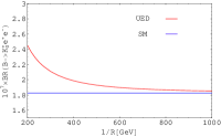
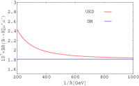
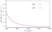
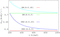
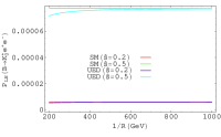
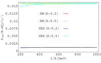
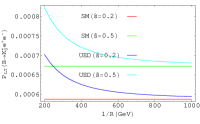
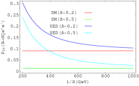
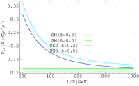
In this section, we numerically analyze the expressions of the branching ratio and double-lepton polarization asymmetries and discuss their dependence and sensitivity on the compactification factor, 1/R1𝑅1/R. Some input parameters of the SM used in the numerical analysis are: mt=167​G​e​Vsubscriptπ‘šπ‘‘167𝐺𝑒𝑉m_{t}=167~{}GeV, mW=80.4​G​e​Vsubscriptπ‘šπ‘Š80.4𝐺𝑒𝑉m_{W}=80.4~{}GeV, mZ=91.18​G​e​Vsubscriptπ‘šπ‘91.18𝐺𝑒𝑉m_{Z}=91.18~{}GeV, mc=1.46​G​e​Vsubscriptπ‘šπ‘1.46𝐺𝑒𝑉m_{c}=1.46~{}GeV, mb=4.8​G​e​Vsubscriptπ‘šπ‘4.8𝐺𝑒𝑉m_{b}=4.8~{}GeV, mu=0.005​G​e​Vsubscriptπ‘šπ‘’0.005𝐺𝑒𝑉m_{u}=0.005~{}GeV, mB=5.28​G​e​Vsubscriptπ‘šπ΅5.28𝐺𝑒𝑉m_{B}=5.28~{}GeV, mK0βˆ—=1.425​G​e​Vsubscriptπ‘šsuperscriptsubscript𝐾01.425𝐺𝑒𝑉m_{K_{0}^{*}}=1.425~{}GeV, s​i​n2​θW=0.23𝑠𝑖superscript𝑛2subscriptπœƒπ‘Š0.23sin^{2}\theta_{W}=0.23, Ξ±e​m=1137subscriptπ›Όπ‘’π‘š1137\alpha_{em}=\frac{1}{137}, Ξ±s​(mZ)=0.118subscript𝛼𝑠subscriptπ‘šπ‘0.118\alpha_{s}(m_{Z})=0.118, |Vt​b​Vt​sβˆ—|=0.041subscript𝑉𝑑𝑏superscriptsubscript𝑉𝑑𝑠0.041|V_{tb}V_{ts}^{*}|=0.041, GF=1.167Γ—10βˆ’5​G​e​Vβˆ’2subscript𝐺𝐹1.167superscript105𝐺𝑒superscript𝑉2G_{F}=1.167\times 10^{-5}~{}GeV^{-2}, me=5.1Γ—10βˆ’4​G​e​Vsubscriptπ‘šπ‘’5.1superscript104𝐺𝑒𝑉m_{e}=5.1\times 10^{-4}~{}GeV, mΞΌ=0.109​G​e​Vsubscriptπ‘šπœ‡0.109𝐺𝑒𝑉m_{\mu}=0.109~{}GeV, mΟ„=1.784​G​e​Vsubscriptπ‘šπœ1.784𝐺𝑒𝑉m_{\tau}=1.784~{}GeV, and Ο„B=1.525Γ—10βˆ’12​ssubscript𝜏𝐡1.525superscript1012𝑠\tau_{B}=1.525\times 10^{-12}s. As we previously mentioned, the branching ratio is obtained integrating the differential decay rate over s^^𝑠\hat{s} in the physical region of the square of the momentum transfered, q2superscriptπ‘ž2q^{2}, hence the obtained expression for the branching ration only depends on the compactification factor. In Fig. 1, we present the dependence branching ratio of the Bβ†’K0βˆ—β€‹l+​lβˆ’β†’π΅superscriptsubscript𝐾0superscript𝑙superscript𝑙B\rightarrow K_{0}^{*}l^{+}l^{-} transition on compactification parameter, 1/R1𝑅1/R in the interval, 200​G​e​V≀1/R≀1000​G​e​V200𝐺𝑒𝑉1𝑅1000𝐺𝑒𝑉200~{}GeV\leq 1/R\leq 1000~{}GeV for different leptons.

Refer to caption
Refer to caption
Refer to caption
Figure 1: The dependence of the branching ratio for Bβ†’K0βˆ—β€‹l+​lβˆ’β†’π΅superscriptsubscript𝐾0superscript𝑙superscript𝑙B\rightarrow K_{0}^{*}l^{+}l^{-} on the compactification factor, 1/R1𝑅1/R for different leptons.

From this figure, we deduce the following results:

  • β€’

    There are considerable discrepancies between the predictions of the ACD and SM models for low values of the compactification factor, 1/R1𝑅1/R. As 1/R1𝑅1/R increases, the difference between the predictions of the two models tends to diminish. The result of ACD approaches the result of SM for higher values of 1/R1𝑅1/R (1/R≃1000​G​e​Vsimilar-to-or-equals1𝑅1000𝐺𝑒𝑉1/R\simeq 1000~{}GeV). Such a discrepancy at low values of 1/R1𝑅1/R can be a signal for the existence of extra dimensions.

  • β€’

    As it is expected, an increase in the lepton mass results in a decrease in the branching ratio. The branching ratios for the e𝑒e and ΞΌπœ‡\mu are approximately the same.

  • β€’

    The order of magnitude of the branching ratio, specially for the e𝑒e and ΞΌπœ‡\mu, depicts a possibility to study such channels at the LHC.
Refer to caption
Refer to caption
Refer to caption
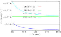
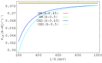
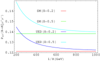
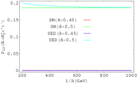
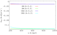
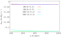
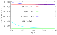
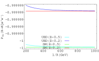
Figure 2: The dependence of the PL​Lsubscript𝑃𝐿𝐿P_{LL} polarization in two models for Bβ†’K0βˆ—β€‹l+​lβˆ’β†’π΅superscriptsubscript𝐾0superscript𝑙superscript𝑙B\rightarrow K_{0}^{*}l^{+}l^{-} on the compactification factor, 1/R1𝑅1/R at different fixed values of s^^𝑠\hat{s} and different leptons.
Refer to caption
Refer to caption
Refer to caption
Figure 3: The same as Fig. 2, but for PL​Nsubscript𝑃𝐿𝑁P_{LN} polarization.
Refer to caption
Refer to caption
Refer to caption
Figure 4: The same as Fig. 2, but for PL​Tsubscript𝑃𝐿𝑇P_{LT} polarization.
Refer to caption
Refer to caption
Refer to caption
Figure 5: The same as Fig. 2, but for PN​Tsubscript𝑃𝑁𝑇P_{NT} polarization.
Refer to caption
Refer to caption
Refer to caption
Figure 6: The same as Fig. 2, but for PT​Tsubscript𝑃𝑇𝑇P_{TT} polarization.
Refer to caption
Refer to caption
Refer to caption
Figure 7: The same as Fig. 2, but for PN​Nsubscript𝑃𝑁𝑁P_{NN} polarization.

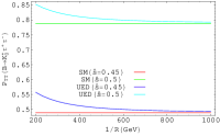
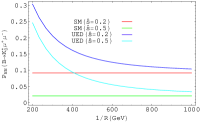
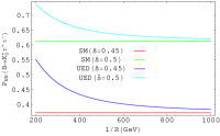
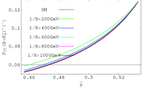
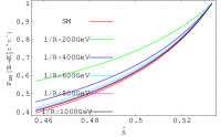
Now, we proceed to show the results of the double-lepton polarization asymmetries. As it is clear from their explicit expressions, they depend on both the compactification factor, 1/R1𝑅1/R and the s^^𝑠\hat{s}. The dependence of different polarization asymmetries on the compactification factor, 1/R1𝑅1/R at different fixed values of s^^𝑠\hat{s} and different leptons are shown in Figs. 2-7. A quick glance at these figures leads to the following conclusions:

  • β€’

    As it is expected, all polarization asymmetries lie between βˆ’11-1 and 111. There are also discrepancies between the predictions of two models for small 1/R1𝑅1/R values, except the PL​Lsubscript𝑃𝐿𝐿P_{LL}, PL​Nsubscript𝑃𝐿𝑁P_{LN} and PN​Tsubscript𝑃𝑁𝑇P_{NT} for e𝑒e and ΞΌπœ‡\mu cases for which the differences between the ACD and SM models are very small. At high values of 1/R1𝑅1/R, two models have approximately the same predictions.

  • β€’

    All double-lepton polarization asymmetries have the same sign for all leptons, except the PL​Lsubscript𝑃𝐿𝐿P_{LL} at which the sign for the Ο„πœ\tau mode is different than those for the e𝑒e and ΞΌπœ‡\mu cases.

  • β€’

    In contrast with the branching ratios, some of the polarization asymmetry predictions are different for the e𝑒e and ΞΌπœ‡\mu cases.

  • β€’

    In PN​Nsubscript𝑃𝑁𝑁P_{NN} for e𝑒e and ΞΌπœ‡\mu and PT​Tsubscript𝑃𝑇𝑇P_{TT} for e𝑒e, the SM gives zero for s^=0.5^𝑠0.5\hat{s}=0.5, while we see considerable nonzero values for them in ACD model at low 1/R1𝑅1/R values.

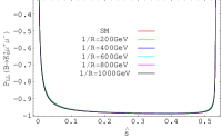
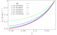
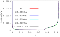
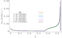
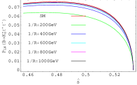
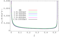
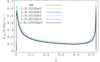
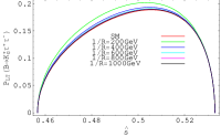
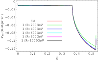
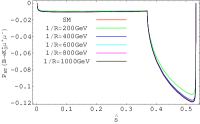
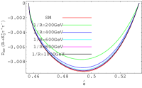
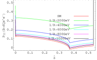
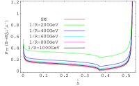
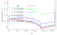
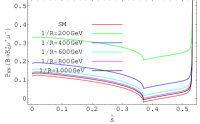
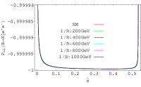
We depict the dependence of the different double-lepton polarization asymmetries on s^^𝑠\hat{s} at different fixed values of 1/R1𝑅1/R and the SM for different leptons in Figs. 8-13. From these figures, we infer the following information:

  • β€’

    The longitudinal-longitudinal polarization asymmetry, PL​Lsubscript𝑃𝐿𝐿P_{LL}, remains approximately unchanged in whole physical region except the end points for the e𝑒e and ΞΌπœ‡\mu. This asymmetry grows as s^^𝑠\hat{s} increases and reaches its maximum at the upper bound of the allowed physical region for Ο„πœ\tau.

  • β€’

    The PL​Nsubscript𝑃𝐿𝑁P_{LN} is zero in the interval, 4​m^l2≀s^≀0.374superscriptsubscript^π‘šπ‘™2^𝑠0.374\hat{m}_{l}^{2}\leq\hat{s}\leq 0.37, but after s^=0.37^𝑠0.37\hat{s}=0.37 it starts to increase up to the upper limit for s^^𝑠\hat{s} ((1βˆ’m^K0βˆ—)2superscript1subscript^π‘šsuperscriptsubscript𝐾0βˆ—2(1-\hat{m}_{K_{0}^{\ast}})^{2}) for e𝑒e and ΞΌπœ‡\mu. For Ο„πœ\tau case, this asymmetry remains approximately unchanged in the interval 4​m^l2≀s^≀0.504superscriptsubscript^π‘šπ‘™2^𝑠0.504\hat{m}_{l}^{2}\leq\hat{s}\leq 0.50, but after this point it starts to diminish and becomes zero at the endpoint.

  • β€’

    The PL​Tsubscript𝑃𝐿𝑇P_{LT} slightly decreases as s^^𝑠\hat{s} increases for the e𝑒e and ΞΌπœ‡\mu cases and has a very small value for the e𝑒e case compared to that of the ΞΌπœ‡\mu. This asymmetry for Ο„πœ\tau, first increases then it decreases after reaching a maximum as s^^𝑠\hat{s} increases in the allowed physical region.

  • β€’

    The normal-transversal polarization asymmetry, PN​Tsubscript𝑃𝑁𝑇P_{NT} remain also unchanged in the interval, 4​m^l2≀s^≀0.374superscriptsubscript^π‘šπ‘™2^𝑠0.374\hat{m}_{l}^{2}\leq\hat{s}\leq 0.37, for e𝑒e and ΞΌπœ‡\mu, but it grows after this interval and has negative sign. In the case of Ο„πœ\tau, this asymmetry also has negative sign and it increases to reach a maximum then decreases as s^^𝑠\hat{s} increases.

  • β€’

    For the e𝑒e and ΞΌπœ‡\mu, the PT​Tsubscript𝑃𝑇𝑇P_{TT} and PN​Nsubscript𝑃𝑁𝑁P_{NN} start to decrease as s^^𝑠\hat{s} increases. The values of these asymmetries in the SM and higher values of the compactification factor become zero around s^=0.37^𝑠0.37\hat{s}=0.37 then they start to increase as s^^𝑠\hat{s} increases. They have minimums at low 1/R1𝑅1/R values at the same s^^𝑠\hat{s}. For Ο„πœ\tau case, the PT​Tsubscript𝑃𝑇𝑇P_{TT} and PN​Nsubscript𝑃𝑁𝑁P_{NN} grow as s^^𝑠\hat{s} increases and the PN​Nsubscript𝑃𝑁𝑁P_{NN} reaches its maximum at the upper bound.

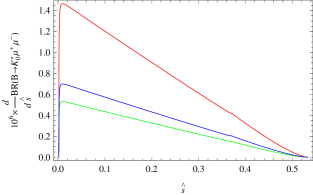
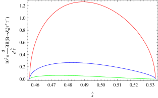
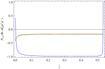
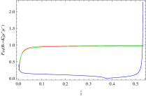
At the end of this section, we would like to quantify the uncertainties of our predictions associated with the errors of the hadronic form factors. In this connection, we show the dependence of the differential branching ratios for ΞΌπœ‡\mu and Ο„πœ\tau on s^^𝑠\hat{s} in Fig. 14 and dependence of PL​Lsubscript𝑃𝐿𝐿P_{LL}, PT​Tsubscript𝑃𝑇𝑇P_{TT} and PN​Nsubscript𝑃𝑁𝑁P_{NN} on s^^𝑠\hat{s} only for ΞΌπœ‡\mu in Fig. 15. These figures contain our predictions (a) in ACD model at 1/R=200​G​e​V1𝑅200𝐺𝑒𝑉1/R=200~{}GeV when the errors presented in Table 1 are added to the central values of the form factors, (b) the same model and 1/R1𝑅1/R, but when the errors of form factors are subtracted from the central values and (c) in SM when central values of the form factors are considered. From Fig. 14, we see that the results of SM lies between the cases (a) and (b) but close to the case (b). In the case of ΞΌπœ‡\mu, the maximum deviation from the SM is in lower values of s^^𝑠\hat{s} and belongs to the case (a) and has the value about two times grater than that of the SM. For Ο„πœ\tau case, the maximum deviation of the ACD prediction lies at middle of the allowed physical region for the s^^𝑠\hat{s}. At this point, the ACD prediction in the case (a) is approximately six times greater than the SM prediction. The similar deviations from the SM model has also been observed for instance in [19] for Ξ›b→Λ​l+​lβˆ’β†’subscriptΛ𝑏Λsuperscript𝑙superscript𝑙\Lambda_{b}\to\Lambda l^{+}l^{-}, but at higher values of s^^𝑠\hat{s}. Figure, 15 depicts an interesting observation. The ACD model in the cases (a) and (b) has approximately the same predictions, but ignoring the end points at which two models have same predictions, the ACD model predictions are 1/5151/5, 555 and approximately 999 times of the SM predictions for PL​Lsubscript𝑃𝐿𝐿P_{LL}, PT​Tsubscript𝑃𝑇𝑇P_{TT} and PN​Nsubscript𝑃𝑁𝑁P_{NN}, respectively.

4 Conclusion

We have calculated some observables such as the branching ratio and double-lepton polarization asymmetries associated with the Bβ†’K0βˆ—β€‹(1430)​l+​lβˆ’β†’π΅superscriptsubscript𝐾01430superscript𝑙superscript𝑙B\rightarrow K_{0}^{*}(1430)l^{+}l^{-} channel in the framework of the ACD model with a single universal extra dimension. We discussed the sensitivities of these observables to the compactification parameter, 1/R1𝑅1/R. We compared the results obtained from the ACD model with the predictions of the standard model. The predictions of the two models approach each other at around 1000​G​e​V1000𝐺𝑒𝑉1000~{}GeV for the value of the compactification parameter, 1/R1𝑅1/R. However the results for the two models differ significantly at lower values of the compactification parameter. This difference grows specially when the errors of the form factors calculated from the QCD sum rules in Table 1 are taken into account. The maximum deviation from the predictions of SM for the considered quantities, obtained using the central values of form factors, belongs to the case of ACD model predictions, where the errors of the form factors are added to the central values of the form factors. This deviation also increases as 1/R1𝑅1/R decreases, such that at low 1/R1𝑅1/R, the discrepancy between predictions of the SM and ACD models reaches to approximately one order of magnitude for some observables. These results beside the other evidences for deviation of the ACD model predictions from the SM obtained via investigating many observables related to the B𝐡B and Ξ›bsubscriptΛ𝑏\Lambda_{b} channels, which due to the heavy bottom quark have large range of q2superscriptπ‘ž2q^{2}, in [5, 6, 8, 10, 11, 12, 13, 19, 20, 21, 22, 23, 24], can be considered as a signal for the existence of extra dimensions in the nature which should we search for in the experiments.

The order of magnitude for the branching ratio shows a possibility to study Bβ†’K0βˆ—β€‹(1430)​l+​lβˆ’β†’π΅superscriptsubscript𝐾01430superscript𝑙superscript𝑙B\rightarrow K_{0}^{*}(1430)l^{+}l^{-} channel at the LHC. Any measurements on the branching ratio as well as the double-lepton polarization asymmetries and determination of their signs and their comparison with the obtained results in this paper can give valuable information about the nature of the scalar meson K0βˆ—β€‹(1430)superscriptsubscript𝐾01430K_{0}^{*}(1430) as well as the possible extra dimensions.
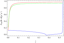
Refer to caption
Refer to caption
Refer to caption
Figure 8: The dependence of the PL​Lsubscript𝑃𝐿𝐿P_{LL} polarization of the Bβ†’K0βˆ—β€‹l+​lβˆ’β†’π΅superscriptsubscript𝐾0superscript𝑙superscript𝑙B\rightarrow K_{0}^{*}l^{+}l^{-} on s^^𝑠\hat{s} at different fixed values of 1/R1𝑅1/R and the SM for different leptons.
Refer to caption
Refer to caption
Refer to caption
Figure 9: The same as Fig. 8, but for PL​Nsubscript𝑃𝐿𝑁P_{LN} polarization.
Refer to caption
Refer to caption
Refer to caption
Figure 10: The same as Fig. 8, but for PL​Tsubscript𝑃𝐿𝑇P_{LT} polarization.
Refer to caption
Refer to caption
Refer to caption
Figure 11: The same as Fig. 8, but for PN​Tsubscript𝑃𝑁𝑇P_{NT} polarization.
Refer to caption
Refer to caption
Refer to caption
Figure 12: The same as Fig. 8, but for PT​Tsubscript𝑃𝑇𝑇P_{TT} polarization.
Refer to caption
Refer to caption
Refer to caption
Figure 13: The same as Fig. 8, but for PN​Nsubscript𝑃𝑁𝑁P_{NN} polarization.
Refer to caption
Refer to caption
Figure 14: The dependence of differential branching ratio for ΞΌπœ‡\mu and Ο„πœ\tau on s^^𝑠\hat{s}. The red color shows the results at 1/R=200​G​e​V1𝑅200𝐺𝑒𝑉1/R=200~{}GeV when the errors of form factors are added to the central values, the green one shows the predictions at the same value of 1/R1𝑅1/R, but when the errors are subtracted from the central values and the blue color shows the result of the SM, when the central value of the form factors are considered
Refer to caption
Refer to caption
Refer to caption
Figure 15: The same as Fig. 14, but for PL​Lsubscript𝑃𝐿𝐿P_{LL}, PT​Tsubscript𝑃𝑇𝑇P_{TT} and PN​Nsubscript𝑃𝑁𝑁P_{NN} polarizations and only for ΞΌπœ‡\mu.

References

  • [1] N. Arkani, S. Dimopoulos, G. Dvali, Phys. Lett. B 429, 263 (1998); Phys. Rev. D 59, 086004 (1999).
  • [2] I. Antoniadis, N. Arkani, S. Dimopoulos, G. Dvali, Phys. Lett. B 439, 257 (1998).
  • [3] I. Antoniadis, Phys. Lett. B 246, 377 (1990).
  • [4] T. Appelquist, H. C. Cheng, B. A. Dobrescu, Phys. Rev. D 64, 035002 (2001).
  • [5] A. J. Buras, M.Spranger, A. Weiler, Nucl. Phys., B 660, (2003) 225.
  • [6] A. J. Buras, A. Poschenrieder, M. Spranger, A. Weiler, Nucl. Phys., B 678,(2004) 455.
  • [7] A. J. Buras, M. Muenz, Phys. Rev., D 52 ,(1995) 186.
  • [8] P. Colangelo, F. De Fazio, R. Ferrandes, T. N. Pham, Phys. Rev. D 73 (2006) 115006.
  • [9] T. Appelquist, H. U. Yee, Phys. Rev. D 67, 055002 (2003).
  • [10] V. Bashiry, M. Bayar, K. Azizi, Phys. Rev. D 78, 035010 (2008).
  • [11] M.V. Carlucci, P. Colangelo, F. De Fazio, Phys. Rev. D 80, 055023 (2009).
  • [12] T. M. Aliev, M. Savci, B. B. Sirvanli, Eur. Phys. J. C 52, 375 (2007).
  • [13] I. Ahmed, M. A. Paracha, M. J. Aslam, Eur. Phys. J. C 54, 591 (2008).
  • [14] M. Misiak, Nucl. Phys., B 393,(1993) 23.
  • [15] T. M. Aliev, K. Azizi, M. Savci, Phys. Rev. D 76, 074017 (2007).
  • [16] T. M. Aliev, V. Bashiry, M. Savci, Eur .Phys. J. C 35 (2004) 197.
  • [17] V. Bashiry, S. M. Zeberjad, F. Falahati, K. Azizi, J. Phys. G 35, 065005 (2008) .
  • [18] S. Fukae, C.S. Kim, T. Yoshikawa, Phys. Rev. D 61 (2000) 074015.
  • [19] Yu-Ming Wang, M. Jamil Aslam, Cai-Dian Lu, Eur. Phys. J. C 59 (2009) 847.
  • [20] P. Colangelo, F. De Fazio, R. Ferrandes, T. N. Pham, Phys. Rev. D 74, 115006 (2006); Phys. Rev. D 77, 055019 (2008).
  • [21] U. Haisch and A. Weiler, Phys. Rev. D 76, 034014 (2007).
  • [22] R. Mohanta and A. K. Giri, Phys. Rev. D 75, 035008 (2007).
  • [23] G. Devidze, A. Liparteliani and U. G. Meissner, Phys. Lett. B 634, 59 (2006).
  • [24] I. I. Bigi, G. G. Devidze, A. G. Liparteliani and U. G. Meissner, Phys. Rev. D 78, 097501 (2008).