Dynamical generation of pseudoscalar resonances

Abstract

We study the interactions between the $f_{0}(980)$ and $a_{0}(980)$ scalar resonances and the lightest pseudoscalar mesons. We first obtain the elementary interaction amplitudes, or interacting kernels, without including any ad hoc free parameter. This is achieved by using previous results on the nature of the lightest scalar resonances as dynamically generated from the rescattering of S-wave two-meson pairs. Afterwards, the interaction kernels are unitarized and the final S-wave amplitudes result. We find that these interactions are very rich and generate a large amount of pseudoscalar resonances that could be associated with the $K(1460)$, $\pi(1300)$, $\pi(1800)$, $\eta(1475)$ and $X(1835)$. We also consider the exotic channels with isospin 3/2 and 1, having the latter positive G-parity. The former could be also resonant in agreement with a previous prediction.

1 Introduction

Due to the spontaneous chiral symmetry breaking of strong interactions [1, 2, 3, 4] strong constraints among the interactions between the lightest pseudoscalars arise, which are most efficiently derived in the framework of Chiral Perturbation Theory (CHPT) [5, 6, 7, 8]. For the isospin ($I$) 0, 1 and 1/2 the scattering of the pseudoscalars in S-wave is strong enough to generate dynamically the lightest scalar resonances, namely, the $f_{0}(980)$, $a_{0}(980)$, $\kappa$ and $\sigma$, as shown in refs. [9, 10, 11, 12, 13]. Still one can make use of the tightly constrained interactions among the lightest pseudoscalars in order to work out approximately the scattering between the latter mesons and scalar resonances, as we show below. We concentrate here on the much narrower resonances $f_{0}(980)$ and $a_{0}(980)$ and consider their interactions with the pseudoscalars $\pi$, $K$, $\eta$ and $\eta^{\prime}$. If these interactions are strong enough new pseudoscalar resonances with $J^{PC}=0^{-+}$ would come up. This is the case and the resulting pseudoscalar resonances have a mass larger than 1 GeV (this energy limit is close to the masses of the $f_{0}(980)$ or $a_{0}(980)$), typically following the relevant scalar-pseudoscalar thresholds.

The problem of the excited pseudoscalars above 1 GeV is interesting by itself. These resonances are not typically well-known [14]. In $I=1/2$ one has the $K(1460)$ and $K(1630)$ resonances. The $I=1$ resonances $\pi(1300)$, $\pi(1800)$ are somewhat better known [14]. They are broad resonances with a large uncertainty in the width of the former, which is reported to range between 200-600 MeV in the PDG [14]. Some controversy exists for interpreting the decay channels of the $\pi(1800)$ within a quarkonium picture [15, 16]. It was suggested in [15] that together with the second radial excitation of the pion there would be a hybrid resonance somewhat higher in mass [15, 17]. Special mention deserves the $I=0$ channel where the $\eta(1295)$, $\eta(1405)$, $\eta(1475)$ have been object of an intense theoretical and experimental study. For an exhaustive review on the experiments performed on these resonances and the nearby $1^{++}$ axial-vector resonance $f_{1}(1420)$ see ref. [18]. Experimentally it has been established that while the $\eta(1405)$ decays mainly to $a_{0}\pi$ the $\eta(1475)$ decays to $K^{*}\bar{K}+c.c$ [14, 18]. In this way, the study of the $\eta\pi\pi$ system is certainly the most adequate one for isolating the $\eta(1405)$ resonance because both the $f_{1}(1420)$ and $\eta(1475)$ have a suppressed partial decay width to this channel [14]. Refs. [14, 18] favor the interpretation of considering the $\eta(1295)$ and $\eta(1475)$ as ideally mixed states (because the $\eta(1295)$ and the $\pi(1300)$ are close in mass) of the same nonet of pseudoscalar resonances with the other members being the $\pi(1300)$ and $K(1460)$. All these resonances would be the first radial excitation of the lightest pseudoscalars [15]. The $\eta(1405)$ would then be an extra state in this classification whose clear signal in gluon-rich process, like $p\bar{p}$ [19, 20] or $J/\Psi$ radiative decays [21, 22], and its absence in $\gamma\gamma$ collision [23], would favor its interpretation as a glueball in QCD [24, 25]. However, this interpretation opens in turn a serious problem because present results from lattice QCD predict the lowest mass for the pseudoscalar glueball at around 2.4 GeV [26, 27, 28]. Given the success of the lattice QCD prediction for the lightest scalar glueball, with a mass at around 1.7 GeV [29, 30], this discrepancy for the pseudoscalar channel would be quite exciting. QCD sum rules [31] give a mass for the lightest pseudoscalar gluonium of $2.05\pm 0.19$ GeV and an upper bound of $2.34\pm 0.42$ GeV. However, the $\eta(1405)$ would fit as a $0^{-+}$ glueball if the latter is a closed gluonic fluxtube [32]. On the other hand, it has also been pointed out that the mass and properties of the $\eta(1405)$ are consistent with predictions for a gluino-gluino bound state [33, 34, 25]. The previous whole picture for classifying the lightest pseudoscalar resonances has been challenged in ref. [16]. The authors question the existence of the $\eta(1295)$ and argue that, due to a node in the ${}^{3}P_{0}$ wave function of the $\eta(1475)$ [35], only one isoscalar pseudoscalar resonance in the 1.4-1.5 GeV region exists. This node shifts the resonant peak position depending on the channel, $a_{0}\pi$ or $K^{*}\bar{K}+c.c$. It has been also recently observed by the BES Collaboration the resonance $X(1835)$ with quantum numbers favored as a pseudoscalar $0^{-+}$ resonance both in $J/\Psi\to\gamma p\bar{p}$ [36] and in $J/\Psi\to\gamma\pi^{+}\pi^{-}\eta^{\prime}$ [37]. For the former decay ref. [38] offers an alternative explanation in terms of the $p\bar{p}$ final state interactions.

We consider here the S-wave interactions between the scalar resonances $f_{0}(980)$ and $a_{0}(980)$ with the pseudoscalar mesons $\pi$, $K$, $\eta$ and $\eta^{\prime}$. The approach followed is an extended version of the one that refs. [39, 40] applied to study the S-wave interactions of the $\phi(1020)$ with the $f_{0}(980)$ and $a_{0}(980)$ resonances, respectively. We show that the interactions derived generate resonances dynamically that can be associated with many of the previous pseudoscalar resonances listed above, namely, with the $K(1460)$, $\pi(1300)$, $\pi(1800)$, $\eta(1475)$ and $X(1835)$. In this way, new contributions to the physical resonant signals result from this novel mechanism not explored so far. In addition, we also study other exotic channels and find that the $I=3/2$ $a_{0}K$ channel could also be resonant.

After this introduction we present the formalism and derive the S-wave scattering amplitudes for scalar-pseudoscalar interactions in section 2. Section 3 is dedicated to present and discuss the results. Conclusions are given in section 4.

2 Formalism. Setting the model

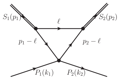
Figure 1: Triangle loop for calculating the interacting kernel for $S_{1}(p_{1})P_{1}(k_{1})\to S_{2}(p_{2})P_{2}(k_{2})$, where between brackets the four-momentum for each particle is given. $S_{1,2}$ represents the initial, final scalar resonances and similarly for $P_{1,2}$ regarding the pseudoscalar mesons.

Our approach is based on the triangle diagram shown in Fig. 1 where an incident scalar resonance $S_{1}$ decays into a virtual $K\bar{K}$ pair. The filled dot in the vertex on the bottom of the diagram corresponds to the interaction of the incident (anti)kaon in the loop with the pseudoscalar $P_{1}$ giving rise to the pseudoscalar $P_{2}$ and the same (anti)kaon. The out-going scalar resonance is denoted by $S_{2}$. The basic point is that this diagram is enhanced because the masses of both the $f_{0}(980)$ and $a_{0}(980)$ resonances are very close to the $K\bar{K}$ threshold. In this way, for scattering near the threshold of the reaction, one of the kaon lines in the bottom of the diagram is almost on-shell. Indeed, at threshold and in the limit for the mass of the scalar equal to twice the kaon mass this diagram becomes infinite. This fact is discussed in detail in ref. [39] where it was already applied for studying successfully the $\phi(1020)f_{0}(980)$ scattering and the associated $1^{--}$ $Y(2175)$ resonance. The BABAR [41] and BELLE [42] data on $e^{+}e^{-}\to\phi(1020)f_{0}(980)$ were reproduced accurately, where a strong peak for the latter resonance arises. An important conclusion of [39] is that the $Y(2175)$ can be qualified as being a resonance dynamically generated due to the interactions between the $\phi(1020)$ and the $f_{0}(980)$ resonances, see also ref. [43]. This work was extended to $I=1$ in [40] for studying the $\phi(1020)a_{0}(980)$ S-wave. There it was remarked the interest of measuring the cross sections $e^{+}e^{-}\to\phi(1020)\pi^{0}\eta$ because it is quite likely that an isovector companion of the $Y(2175)$ appears. In our present study, as well as in refs. [39, 40], one takes advantage of the fact that both the $f_{0}(980)$ and $a_{0}(980)$ resonances are dynamically generated by the meson-meson self-interactions [9, 13, 44]. This conclusion is also shared with other approaches like refs. [45, 46]. In this way, we can calculate the couplings of the scalar resonances considered to two pseudoscalars, including their relative phase. The coupling of the $f_{0}(980)$ and $a_{0}(980)$ resonances to a $K\bar{K}$ pair in $I=0$ and 1, respectively, is denoted by $g_{f_{0}}$ and $g_{a_{0}}$. These states $|K\bar{K}\rangle_{I=0}$ and $|K\bar{K}\rangle_{I=1}$ are given by

$$|K\bar{K}\rangle_{I=0} =-\frac{1}{\sqrt{2}}|K^{+}K^{-}+K^{0}\bar{K}^{0}\rangle~{},$$

$$|K\bar{K}\rangle_{I=1} =-\frac{1}{\sqrt{2}}|K^{+}K^{-}-K^{0}\bar{K}^{0}\rangle~{}.$$ (2.1)

In this way, the $f_{0}(980)$ couples to $K^{+}K^{-}$($K^{0}\bar{K}^{0}$) as $-\frac{1}{\sqrt{2}}$($-\frac{1}{\sqrt{2}})g_{f_{0}}$ while the $a_{0}(980)$ couples as $-\frac{1}{\sqrt{2}}(\frac{1}{\sqrt{2}})g_{a_{0}}$.

Let us indicate by $P$ the total four-momentum $P=p_{1}+k_{1}=p_{2}+k_{2}$ in Fig. 1. This diagram is given by $g_{1}g_{2}L_{K}$, with $g_{1}$ and $g_{2}$ the coupling of the initial and final scalar resonance to a $K\bar{K}$ pair, respectively, and $L_{K}$ is given by

$$L_{K} =i\int\frac{d^{4}\ell}{(2\pi)^{4}}\frac{T((P-\ell)^{2})}{(\ell^{2}-m_{K}^{2}+i\varepsilon)((p_{1}-\ell)^{2}-m_{K}^{2}+i\varepsilon)((p_{2}-\ell)^{2}-m_{K}^{2}+i\varepsilon)}~{}.$$ (2.2)

In this equation $T((P-\ell)^{2})$ represents the interaction amplitude between the kaons with the external pseudoscalars. Here, we employ the meson-meson scattering amplitudes obtained in ref. [13] but now enlarged so that states with the pseudoscalar $\eta^{\prime}$ are included in the calculation of $T((P-\ell)^{2})$, as detailed in appendix A. Interestingly, these amplitudes contain the poles corresponding to the scalar resonances $\sigma$, $\kappa$, $f_{0}(980)$, $a_{0}(980)$ and other poles in the region around 1.4 GeV [13].

In order to proceed further we have to know the dependence of $T((P-\ell)^{2})$ on its argument that includes the integration variable $\ell$. This can be done by writing the dispersion relation satisfied by $T(q^{2})$ which is of the form

$$T(q^{2}) =T(s_{A})+\sum_{i}\frac{q^{2}-s_{A}}{q^{2}-s_{i}}\frac{\hbox{Res}_{i}}{s_{i}-s_{A}}+\frac{q^{2}-s_{A}}{\pi}\int_{s_{th}}^{\infty}ds^{\prime}\frac{\hbox{Im}T(s^{\prime})}{(s^{\prime}-q^{2})(s^{\prime}-s_{A})}~{}.$$ (2.3)

One subtraction at $s_{A}$ has been taken because $T(q^{2})$ is bound by a constant for $q^{2}\to\infty$, with $T(s_{A})$ the subtraction constant. Typically, poles are also present deep in the $q^{2}$-complex plane located at $s_{i}$ whose residues are Res_i. These poles appear on the first Riemann sheet and are an artifact of the parameterization employed [13, 47]. For $q^{2}$ along the physical region they just give rise to soft extra contributions that could be mimic by a polynomial of low degree in $q^{2}$. Inserting eq. (2.3) into eq. (2.2), with $(P-\ell)^{2}=q^{2}$, one can write for $L_{K}$

$$L_{K} =\left(T(s_{A})+\sum\frac{\hbox{Res}_{i}}{s_{i}-s_{A}}\right)C_{3}+\sum_{i}C_{4}(s_{i})\hbox{Res}_{i}$$

$$-\frac{1}{\pi}\int_{s_{th}}^{\infty}ds^{\prime}\hbox{Im}T(s^{\prime})\left[\frac{C_{3}}{s^{\prime}-s_{A}}+C_{4}(s^{\prime})\right]~{}.$$ (2.4)

Here we have introduced the three- and four-point Green functions $C_{3}$ and $C_{4}(M_{4}^{2})$ defined by

$$C_{3} =i\int\frac{d^{4}\ell}{(2\pi)^{4}}\frac{1}{(\ell^{2}-m_{K}^{2}+i\varepsilon)((p_{1}-\ell)^{2}-m_{K}^{2}+i\varepsilon)((p_{2}-\ell)^{2}-m_{K}^{2}+i\varepsilon)}~{},$$

$$C_{4}(M_{4}^{2}) =i\int\frac{d^{4}\ell}{(2\pi)^{4}}\frac{1}{(\ell^{2}-m_{K}^{2}+i\varepsilon)((p_{1}-\ell)^{2}-m_{K}^{2}+i\varepsilon)((p_{2}-\ell)^{2}-m_{K}^{2}+i\varepsilon)}$$

$$\times\frac{1}{((P-\ell)^{2}-M_{4}^{2}+i\epsilon)}~{}.$$ (2.5)

Notice that $M_{4}^{2}$ can be real positive (when $M_{4}^{2}=s^{\prime}$ in the dispersion relation), but it could also be negative or even complex when $M_{4}^{2}=s_{i}$ from the poles. One has still to perform the angular projection for $C_{3}$ and $C_{4}(M_{4}^{2})$. Once this is done, eq. (2.4) can still be used but with $C_{3}$ and $C_{4}(M_{4}^{2})$ projected in S-wave, as we take for granted in the following. These functions and their S-wave projection are discussed in appendix B. For $S_{1}(p_{1})P_{1}(k_{1})\to S_{2}(p_{2})P_{2}(k_{2})$ we have the usual Mandelstam variables $s=(p_{1}+k_{1})^{2}=(p_{2}+k_{2})^{2}$, $t=(p_{1}-p_{2})^{2}=(k_{1}-k_{2})^{2}$ and $u=(p_{1}-k_{2})^{2}=(p_{2}-k_{1})^{2}=M_{S_{1}}^{2}+M_{S_{2}}^{2}+M_{P_{1}}^{2}+M_{P_{2}}^{2}-s-t$, with the masses of the particles indicated by $M$ with the subscript distinguishing between them. The dependence on the relative angle $\theta$ enters in $t$ as $t=(p_{1}^{0}-k_{1}^{0})^{2}-(\mathbf{p}-\mathbf{p}^{\prime})^{2}=(p_{1}^{0}-k_{1}^{0})^{2}-\mathbf{p}^{2}-\mathbf{p}^{\prime 2}+2|\mathbf{p}||\mathbf{p}^{\prime}|\cos\theta$ with $\mathbf{p}$ and $\mathbf{p}^{\prime}$ the CM three-momentum of the initial and final particles, respectively.

Eq. (2.4) is our basic equation for evaluating the interaction kernels. One has only to specify the pseudoscalars actually involved in the amplitude $T(q^{2})$ according to the specific reaction under consideration. We now list all the channels involved for the different quantum numbers and indicate the actual pseudoscalar-pseudoscalar amplitudes required as the argument of $L_{K}$:

• $I=0$, $G=+1$

  $$T_{L}(a_{0}\pi\to a_{0}\pi) =\frac{2g_{a_{0}}^{2}}{3}L_{K}[4\,T_{\pi K\to\pi K}^{I=3/2}-T_{\pi K\to\pi K}^{I=1/2}]~{},$$

  $$T_{L}(a_{0}\pi\to f_{0}\eta) =2g_{f_{0}}g_{a_{0}}L_{K}[T_{\eta K\to\pi K}^{I=1/2}]~{},$$

  $$T_{L}(f_{0}\eta\to f_{0}\eta) =2g_{f_{0}}^{2}L_{K}[T_{\eta K\to\eta K}^{I=1/2}]~{},$$

  $$T_{L}(a_{0}\pi\to f_{0}\eta^{\prime}) =2g_{f_{0}}g_{a_{0}}L_{K}[T_{\eta^{\prime}K\to\pi K}^{I=1/2}]~{},$$

  $$T_{L}(f_{0}\eta\to f_{0}\eta^{\prime}) =2g_{f_{0}}^{2}L_{K}[T_{\eta K\to\eta^{\prime}K}^{I=1/2}]~{},$$

  $$T_{L}(f_{0}\eta^{\prime}\to f_{0}\eta^{\prime}) =2g_{f_{0}}^{2}L_{K}[T_{\eta^{\prime}K\to\eta^{\prime}K}^{I=1/2}]~{}.$$ (2.6)

• $I=1/2$

  $$T_{L}(f_{0}K\to f_{0}K) =\frac{g_{f_{0}}^{2}}{2}L_{K}[3\,T_{K\bar{K}\to K\bar{K}}^{I=1}+T_{K\bar{K}\to K\bar{K}}^{I=0}]~{},$$

  $$T_{L}(f_{0}K\to a_{0}K) =\frac{\sqrt{3}g_{f_{0}}g_{a_{0}}}{2}L_{K}[T_{K\bar{K}\to K\bar{K}}^{I=1}-T_{K\bar{K}\to K\bar{K}}^{I=0}]~{},$$

  $$T_{L}(a_{0}K\to a_{0}K) =\frac{g_{a_{0}}^{2}}{2}L_{K}[3\,T_{K\bar{K}\to K\bar{K}}^{I=0}+T_{K\bar{K}\to K\bar{K}}^{I=1}]~{}.$$ (2.7)

• $I=1$, $G=-1$

  $$T_{L}(f_{0}\pi\to f_{0}\pi) =\frac{2g_{f_{0}}^{2}}{3}L_{K}[2\,T_{\pi K\to\pi K}^{I=3/2}+T_{\pi K\to\pi K}^{I=1/2}]~{},$$

  $$T_{L}(f_{0}\pi\to a_{0}\eta) =\frac{2g_{f_{0}}g_{a_{0}}}{\sqrt{3}}L_{K}[T_{\pi K\to\eta K}^{1/2}]~{},$$

  $$T_{L}(a_{0}\eta\to a_{0}\eta) =2g_{a_{0}}^{2}L_{K}[T_{\eta K\to\eta K}^{I=1/2}]~{},$$

  $$T_{L}(f_{0}\pi\to a_{0}\eta^{\prime}) =\frac{2g_{f_{0}}g_{a_{0}}}{\sqrt{3}}L_{K}[T_{\pi K\to\eta^{\prime}K}^{I=1/2}]~{},$$

  $$T_{L}(a_{0}\eta\to a_{0}\eta^{\prime}) =2g_{a_{0}}^{2}L_{K}[T_{\eta K\to\eta^{\prime}K}^{I=1/2}]~{},$$

  $$T_{L}(a_{0}\eta^{\prime}\to a_{0}\eta^{\prime}) =2g_{a_{0}}^{2}L_{K}[T_{\eta^{\prime}K\to\eta^{\prime}K}^{I=1/2}]~{}.$$ (2.8)

• $I=1$, $G=+1$

  $$T_{L}(a_{0}\pi\to a_{0}\pi) =\frac{2g_{a_{0}}^{2}}{3}L_{K}[4T_{\pi K\to\pi K}^{I=1/2}-T_{\pi K\to\pi K}^{I=3/2}]~{}.$$ (2.9)

• $I=3/2$

  $$T_{L}(a_{0}K\to a_{0}K) =2g_{a_{0}}^{2}L_{K}[T_{K\bar{K}\to K\bar{K}}^{I=1}]~{}.$$ (2.10)

In the previous equations the different scalar-pseudoscalar states are pure isospin ones corresponding to the isospin $I$ indicated for each item. This also applies to the pseudoscalar-pseudoscalar states, with $I$ as indicated in the superscript of $T$. The symbol $G$ refers to G-parity. On the other hand the $I=3/2$ $\pi K$ amplitude, being much smaller than the $I=1/2$ one, has negligible effects, although it has been kept in the previous expressions.

Figure 2: Iteration of the interaction kernels (denoted by the triangles in the figure) by inserting scalar(double lines)-pseudoscalar(dashed lines) intermediate states.

For each set of quantum numbers specified by the isospin $I$ and G-parity $G$ (if the latter is not defined this label should be omitted) we join in a symmetric matrix ${\cal T}_{IG}$ the different $T_{L}(i\to j)$ calculated above. Then, in order to resum the unitarity loops, as indicated in Fig. 2, and obtain the final S-wave scalar-pseudoscalar T-matrix, $T_{IG}$, we make use of the equation

$$T_{IG} =\left[I+{\cal T}_{IG}\cdot g_{IG}(s)\right]^{-1}\cdot{\cal T}_{IG}~{}.$$ (2.11)

For a general derivation of this equation, based on the N/D method [48], see refs. [13, 49] and ref. [9], where it is connected with the Bethe-Salpeter equation. In eq. (2.11) $g_{IG}(s)$ is a diagonal matrix whose elements are the scalar unitarity loop function with a scalar-pseudoscalar intermediate state. For the calculation of $g_{IG}(s)_{i}$, corresponding to the $i_{th}$ state with the quantum numbers $IG$ and made up by the scalar resonance $S_{i}$ and the pseudoscalar $P_{i}$, we make use of a once subtracted dispersion relation [13]. The result is

$$g_{IG}(s)_{i} =\frac{1}{(4\pi)^{2}}\left\{a_{1}+\log\frac{M_{S_{i}}^{2}}{\mu^{2}}-\frac{M_{P_{i}}^{2}-M_{S_{i}}^{2}+s}{2s}\log\frac{M_{S_{i}}^{2}}{M_{P_{i}}^{2}}\right.$$

$$\left.+\frac{|\mathbf{p}|}{\sqrt{s}}\Biggl{[}\log(s-\Delta+2\sqrt{s}|\mathbf{p}|)+\log(s+\Delta+2\sqrt{s}|\mathbf{p}|)\right.$$

$$\left.-\log(-s+\Delta+2\sqrt{s}|\mathbf{p}|)-\log(-s-\Delta+2\sqrt{s}|\mathbf{p}|)\Biggr{]}\right\}$$ (2.12)

with $|\mathbf{p}|$ the three-momentum of the channel $S_{i}P_{i}$ for a given $s$ and $\Delta=M_{P_{i}}^{2}-M_{S_{i}}^{2}$. The subtraction $a_{1}$ is restricted to have natural values so that the unitarity scale [39] $4\pi f_{\pi}/\sqrt{|a_{1}|}$ becomes not too small (e.g. below the $\rho$-mass) so that $|a_{1}|\lesssim 3$. In addition, we require the sign of $a_{1}$ to be negative so that resonances could be generated when the interaction kernel is positive (attractive).

As already indicated in ref. [40] to ensure a continuous limit to zero $a_{0}(980)$ width, one has to evaluate ${\cal T}_{IG}$ at the $a_{0}(980)$ pole position with positive imaginary part so that $p_{1,2}^{2}\to{\rm Re}\,[M_{a_{0}}]^{2}+i\epsilon$, in agreement with Eq. (2.2). Instead, in $g_{IG}(s)_{a_{0}P}$, with $P$ one of the lightest pseudoscalars, $M_{a_{0}}$ should appear with a negative imaginary part to guarantee that, in the zero-width limit, the sign of the imaginary part is the same as dictated by the $-i\epsilon$ prescription for masses squared of the intermediate states. Such analytical extrapolations in the masses of external particles are discussed in Refs. [50, 51, 52]. The same applies of course to the case of the $f_{0}(980)$ resonance.

3 Results

In this section we show the results that follow by applying eq. (2.11) to the different channels characterized by the quantum numbers $IG$, as given in the list from eq. (2.6) to eq. (2.10). As discussed after eq. (2.12) we consider values for the subtraction constant such that they are negative and not very large in modulus ($|a_{1}|\lesssim 3$). In this way, the resonances generated might be qualified as dynamically generated due to the iteration of the unitarity loops. The pole positions and couplings of the $f_{0}(980)$ and $a_{0}(980)$ resonances are given in Tables 3 and 4, respectively, and they correspond to those obtained in the meson-meson S-wave amplitudes used, see appendix A. We present the results for each of the channels with definite $IG$ separately.

Figure 3: Modulus squared of the $f_{0}K\to f_{0}K$ (left) and $a_{0}K\to a_{0}K$ (right) S-wave amplitudes for $a_{1}=-0.5$ . The points correspond to the energies where the amplitudes have been actually calculated.

3.1 $I=1/2$

First we show the results for the $I=1/2$ sector that couples together the channels $f_{0}(980)K$ and $a_{0}(980)K$. We show the modulus squared of the $f_{0}K\to f_{0}K$ and $a_{0}K\to a_{0}K$ S-wave amplitudes in the left and right panel of Fig. 3, respectively. We obtain a clear resonant peak with its maximum at $1460$ MeV for $a_{1}$ around $-0.5$, that corresponds to the nominal mass of the $K(1460)$ resonance [14]. The results are not very sensitive to the actual value of $a_{1}$ but the position of the peak displaces to lower values for decreasing $a_{1}$ and the width somewhat increases. The visual width of the peak is around 100 MeV, although it appears wider in $a_{0}K\to a_{0}K$ scattering. In refs. [53, 54] a larger width of around 250 MeV is referred. One has to take into account that the channel $K^{*}(892)\pi$ is not included and it seems to couple strongly with the $K(1460)$ resonance [14]. It is also clear from the figure that the peak is asymmetric due to the opening of the $f_{0}K$ and $a_{0}K$ thresholds involved. Taking into account the relative sizes of the peaks in the left and right panels of Fig. 3 one infers that the $K(1460)$ couples more strongly to $f_{0}K$ than to $a_{0}K$, with the ratio of couplings as $|g_{f_{0}K}/g_{a_{0}K}|\simeq(\frac{20.2}{5.7})^{1/4}\simeq 1.4$ .

Figure 4: Modulus squared of the $a_{0}\eta^{\prime}\to a_{0}\eta^{\prime}$ (left) and $a_{0}\eta\to a_{0}\eta$ (right) S-wave amplitudes. For the former $a_{1}=-1.3$ and for the latter $a_{1}=-2.0$, see the text for details. The notation is as in Fig. 3.

3.2 $I=1$

We now consider the $I=1$ case. As commented in the introduction two broad resonances are referred in the PDG, the $\pi(1300)$ and $\pi(1800)$. In our amplitudes we find quite independently of the value of $a_{1}$ that the $a_{0}(980)\eta^{\prime}$ channel is almost elastic. This is due to the fact that the interaction kernels ${\cal T}(a_{0}\eta^{\prime}\to a_{0}\eta)$ and ${\cal T}(a_{0}\eta^{\prime}\to f_{0}\pi)$ are much smaller than the rest of kernels, typically by an order of magnitude. This happens because the kernels are dominated by the threshold region. However, the threshold for $a_{0}(980)\eta^{\prime}$ is much higher than the thresholds for the other two channels. In this way, for the inelastic processes involving the $a_{0}\eta^{\prime}$ channel, even at threshold for one of the channels, there is always a large three-momentum for the other channel and the kernel is suppressed. Of course, this does not apply for the $a_{0}\eta^{\prime}$ elastic case where the kernel has a standard size and produces around 1.8 GeV a strong resonant signal that could be associated with the $\pi(1800)$ resonance. To reproduce the mass value given in the PDG [14] for this resonance, $1816\pm 14$ MeV one takes $a_{1}$ for $a_{0}\eta^{\prime}$ around -1.3. The visual width of the peak is around 200 MeV, close to the width quoted in the PDG [14] of $208\pm 12$ MeV. The other two channels couple quite strongly between each other and typically give rise to an enhancement between 1.2-1.4 GeV when varying $a_{1}$ equal for each of them, which could be associated with the $\pi(1300)$. However, for $|a_{1}|$ between 1 and 1.8 a too strong signal in the $a_{0}\eta$ threshold originates. For $|a_{1}|$ below 1 the resonant peak in the $|T(a_{0}\eta\to a_{0}\eta)|^{2}$ lies around 1.4-1.5 GeV, somewhat too high for the $\pi(1300)$ resonance [14]. This is why we show in Fig. 4 the modulus squared of $a_{0}\eta\to a_{0}\eta$ for $a_{1}=-2$ where a peak close to 1.2 GeV is seen with a width of around 200 MeV. One can also see the strong effect of the $a_{0}\eta$ threshold at around 1.52 GeV. Its size is rather sensitive to the actual vale of $|a_{1}|$ when this lies between 1 and 1.8. There is the interesting fact, which is independent of the value of $a_{1}$, that there is no signal for $\pi(1800)$ in the $a_{0}\eta$ system nor signal of the peak at 1.2 GeV in the $a_{0}\eta^{\prime}$. We have also checked that this is also the case for the $f_{0}\pi$ state, that is, it does not couple with the $\pi(1800)$. This is another reflection of the fact that the $a_{0}\eta^{\prime}$ tends to decouple from the other states.

Figure 5: Modulus squared of the $f_{0}\eta^{\prime}\to f_{0}\eta^{\prime}$ (left) and $f_{0}\eta\to f_{0}\eta$ (right) S-wave amplitudes. For the former $a_{1}=-1.25$ and for the latter $a_{1}=-0.8$, see the text for details. The notation is as in Fig. 3.

3.3 $I=0$

We move next to the $I=0$ system where the $f_{0}\eta$, $a_{0}\pi$ and $f_{0}\eta^{\prime}$ couple. Here occurs similarly to $I=1$, so that the much higher $f_{0}\eta^{\prime}$ channel mostly decouples from the other two channels. We then proceed similarly and distinguish between the subtraction constant $a_{1}$ attached to $a_{0}\eta^{\prime}$ and to the other two channels $a_{0}\pi$ and $f_{0}\eta$. For $a_{1}$ around $-1.2$ one obtains a resonance of the $a_{0}\eta^{\prime}$ channel at a mass of 1835 MeV, in agreement with that quoted in the PDG for the $X(1835)$, $1833.7\pm 6.1\pm 2.7$ MeV. This is shown in the left panel of Fig. 5 where the modulus squared of the $f_{0}(980)\eta^{\prime}\to f_{0}(980)\eta^{\prime}$ S-wave amplitude is shown. The width of the peak at half its maximum value is around 70 MeV, in good agreement with the width given in the PDG for the $X(1835)$ of $67.7\pm 20.3\pm 7.7$ MeV. We consider next the other two coupled channels, $a_{0}(980)\pi$ and $f_{0}(980)\eta$. We obtain a clear resonant signal with mass around 1.45 GeV for $|a_{1}|\lesssim 1$. This is shown in the right panel of Fig. 5, where the modulus squared of the $f_{0}(980)\eta\to f_{0}(980)\eta$ is given for $a_{1}=-0.8$. It is not possible to increase further the mass of this peak by varying $a_{1}$. An important fact of this resonance is that it does not couple to the $a_{0}\pi$ channel. E.g. the analogous curve for the modulus squared of the $a_{0}(980)\pi\to a_{0}(980)\pi$ S-wave in the 1.4 GeV region is absolutely flat. By considering the inelastic process $f_{0}(980)\eta\to a_{0}(980)\pi$ we estimate a coupling to the latter channel more than 14 times smaller than to $f_{0}(980)\eta$. Because the $\eta(1405)$ resonance couples mostly to $a_{0}(980)\pi$ [14] we then conclude that the generated resonant signal around $1.45$ GeV should correspond to the $\eta(1475)$. Its form is rather asymmetric due to the opening of the $f_{0}(980)\eta$ threshold, with a width at half the maximum of its peak of around 150 MeV. The width quoted in the PDG [14] is $85\pm 9$ MeV. It is also known that the $\eta(1475)$ couples strongly to $K^{*}(892)\bar{K}+c.c$, a channel not included in our study. The threshold for this channel, at around 1.39 GeV at the decreasing slop of our present signal, should certainly modify its shape. For higher values of $|a_{1}|$ the peak tends to become too light in mass compared with the $\eta(1475)$. For the $a_{0}(980)\pi\to a_{0}(980)\pi$ reaction one also appreciates a strong $a_{0}(980)\pi$ threshold effect at around 1.16 GeV. No resonance around the mass of the $\eta(1295)$ is observed.

Figure 6: Modulus squared of the $I=3/2$ $a_{0}K\to a_{0}K$ S-wave amplitude with $a_{1}=-0.5$. The notation is as in Fig. 3.

Resonance	$I^{(G)}$	Width (MeV)	Comments
$K(1460)$	$I=\frac{1}{2}$	$\Gamma\gtrsim 100$	$|g_{f_{0}K}/g_{a_{0}K}|\simeq 1.4$
$\pi(1800)$	$I^{G}=1^{-}$	$\Gamma\simeq 200$	$a_{0}\eta^{\prime}$ elastic
$\pi(1300)$	$I^{G}=1^{-}$	$\Gamma\gtrsim 200$	$a_{0}\pi$, $f_{0}\eta$ coupled channels
$X(1835)$	$I^{G}=0^{+}$	$\Gamma\simeq 70$	$f_{0}\eta^{\prime}$ elastic
$\eta(1475)$	$I^{G}=0^{+}$	$\Gamma\simeq 150$	$f_{0}\eta$ elastic
Exotic	$I=\frac{3}{2}$	$\Gamma\simeq 200$	$a_{0}K$ threshold

Table 1: Resonances resulting from our study. For more details see the discussions of the results in the text.

3.4 Exotic channels

Regarding the exotic channel with $I=3/2$ we find an interesting result. Our amplitude gives rise to a clear resonant structure at around 1.4 GeV for $|a_{1}|\lesssim 1.5$. We show the modulus squared of $T(a_{0}^{\pm}K^{\pm}\to a_{0}^{\pm}K^{\pm})$, because the $a_{0}^{\pm}K^{\pm}$ states are purely $I=3/2$, for $a_{1}=-0.5$ (the same value used before in Fig. 3 studying the $I=1/2$ case) in Fig. 6. One also observes that the shape of the resonance peak is asymmetric with a clear impact of the $a_{0}K$ threshold. Our results for $|a_{1}|\lesssim 1$ tends to confirm the predictions of Longacre [55] that studied the $K\bar{K}\pi$ and $K\bar{K}K$ system and concluded that the exotic $I=3/2$ $J^{P}=0^{-}$ $K\bar{K}K$ system was resonant around its threshold due to the successive interactions between a $K$, $\bar{K}$ and a $\pi$. For $|a_{1}|\gtrsim 1$ we find that the resonance shape in $|T(a_{0}^{\pm}K^{\pm}\to a_{0}^{\pm}K^{\pm})|^{2}$ progressively distorts becoming lighter and flatter. Let us notice also that the $a_{0}K$ system was not isolated in the two experiments quoted in the PDG where the $I=1/2$ $K(1460)$ was observed [53, 54].

The other exotic channel with $I=1$ and $G=+1$ involves the isovector $a_{0}\pi$ state. Whether a resonance behavior stems at around 1.4 GeV depends on the actual value of $a_{1}$. For $|a_{1}|\lesssim 1$ the enhancement near 1.4 GeV is much weaker and is overcome by the cusp effect at the $a_{0}\pi$ threshold. For larger values of $|a_{1}|$ the resonant signal is much more prominent. No such resonance has been found experimentally, e.g. in peripheral hadron production [56], so that $|a_{1}|\lesssim 1$ should be finally taken.

In Table 1 we collect all the resonances found in our study for the different quantum numbers discussed.

4 Summary and conclusions

In summary, we have presented a study of the S-wave interactions between the scalar resonances $f_{0}(980)$ and $a_{0}(980)$ with the lightest pseudoscalars ($\pi$, $K$, $\eta$ and $\eta^{\prime}$) in the region between 1 and 2 GeV. The different channels studied comprise those alike the $\eta$, $K$ and $\pi$, and the exotic ones with isospin 3/2 and 1, the latter having positive G-parity. First, interaction kernels have been derived by considering the interactions of the external pseudoscalars involved in the reaction with those making the scalar resonance. We take advantage here of previous studies that establish the $f_{0}(980)$ and $a_{0}(980)$ as dynamically generated from the interactions of two pseudoscalars, so that no free parameters are introduced in their calculation. Afterwards, the final S-wave amplitudes are determined by employing techniques borrowed from Unitary Chiral Perturbation Theory. Interestingly, we have obtained resonant peaks that for the non-exotic channels could be associated with the pseudoscalar resonances $K(1460)$, $\pi(1300)$, $\pi(1800)$, $\eta(1475)$ and $X(1835)$, following the notation of the particle data group. The resonances that come out from this study can be qualified as dynamically generated from the interactions between the scalar resonances and the pseudoscalar mesons. This establishes that an important contribution to the physical signal of the resonances just mentioned has a dynamical origin. The exotic $I=3/2$ channel could also exhibit a resonant structure around the $a_{0}K$ threshold, in agreement with the behavior predicted by Longacre [55] twenty years ago. However, larger values for the subtraction constant $|a_{1}|$ tends to destroy this resonant behavior. No signal of the intriguing $\eta(1405)$ resonance is obtained.

This approach should be pursued further by including simultaneously to the interaction between the scalar resonances and the pseudoscalar mesons, considered here, those arising from the lightest vector resonances with the same pseudoscalars in P-wave. In this way, both pseudoscalar and axial resonances will be studied together.

Appendix A Meson–meson unitarized amplitudes

We use the $N/D$ method [13] to unitarize the different isospin channels amplitudes for meson–meson scattering, which are fitted to data, and then used in the vertex of the triangle loop. From these amplitudes, once fitted, the position of the poles can be found (we use here the $f_{0}(980)$ and $a_{0}(980)$, but we also check for the appearance of the other scalars, $\sigma$ and $\kappa$). As mentioned, the amplitudes are unitarized through

$$T_{I}=(1+V_{I}\cdot G)^{-1}\cdot V_{I}~{},$$ (A.1)

which is analogous to eq. (2.11) but now for the pseudoscalar-pseudoscalar scattering. The symmetric matrix $V_{I}$ (the analogous one to ${\cal T}_{IG}$ in eq. (2.11)) collects the S-wave pseudoscalar-pseudoscalar tree-level amplitudes obtained from the lowest order Chiral Lagrangians including resonances as well. The matrix $G$ is a diagonal matrix that contains the meson–meson loop propagator (the same expression as given in eq. (2.12) can be used with the appropriate replacement for the masses involved.)

The lowest order chiral Lagrangian at leading order in large $N_{c}$ which also includes the $\eta_{1}$ is [57, 58, 59]

$$\mathcal{L}_{2} = \frac{f_{\pi}^{2}}{4}\langle\partial_{\mu}U^{\dagger}\partial^{\mu}U\rangle+\frac{f_{\pi}^{2}}{4}\langle\chi^{\dagger}U+\chi U^{\dagger}\rangle-\frac{1}{2}M_{1}^{2}\eta_{1}^{2}~{},$$ (A.2)

$$U(\phi) = \exp\left(i\sqrt{2}\Phi/f_{\pi}\right)\text{,}\quad\Phi=\sum_{i=0}^{8}\frac{\lambda_{i}}{\sqrt{2}}\phi_{i}\text{,}\quad\lambda_{0}=\sqrt{\frac{2}{3}}\mathbf{I}_{3}~{},$$ (A.3)

and $\lambda_{i}$, $i=1,\ldots,8$ the Gell-Mann matrices. The $\eta_{8}$ and $\eta_{1}$ fields mix to give the physical $\eta$ and $\eta^{\prime}$

$$\left(\begin{array}[]{c}\eta^{\prime}\\ \eta\end{array}\right)=\left(\begin{array}[]{cc}\cos{\theta}&\sin{\theta}\\ -\sin{\theta}&\cos{\theta}\end{array}\right)\left(\begin{array}[]{c}\eta_{1}\\ \eta_{8}\end{array}\right)~{}.$$

The mixing angle $\theta$ is taken as $\sin\theta\simeq-\frac{1}{3}$, $\theta\simeq-20^{\circ}$ [60].

In the same spirit as in ref. [13] the explicit exchange of $J^{PC}=0^{++}$ scalar resonances is incorporated and calculated from the leading order chiral Lagrangians of ref. [61]. The appropriate Lagrangians are

$$\mathcal{L}_{S_{8}} = c_{d}\left\langle S_{8}u_{\mu}u^{\mu}\right\rangle+c_{m}\left\langle S_{8}\chi_{+}\right\rangle~{},$$ (A.4)

$$\mathcal{L}_{S_{1}} = \tilde{c}_{d}S_{1}\left\langle u_{\mu}u^{\mu}\right\rangle+\tilde{c}_{m}S_{1}\left\langle\chi_{+}\right\rangle~{},$$

$$\chi_{+} = u^{\dagger}\chi u^{\dagger}+u\chi^{\dagger}u~{},$$

$$U(x) = u(x)^{2}\text{,}\quad u_{\mu}=iu^{\dagger}\partial_{\mu}Uu^{\dagger}=u_{\mu}^{\dagger}~{},$$

$$S_{8} = \left(\begin{array}[]{ccc}\frac{a_{0}}{\sqrt{2}}+\frac{f_{8}}{\sqrt{6}}&a_{0}^{+}&{K^{*}_{0}}^{+}\\ a_{0}^{-}&-\frac{a_{0}}{\sqrt{2}}+\frac{f_{8}}{\sqrt{6}}&{K^{*}_{0}}^{0}\\ {K^{*}_{0}}^{-}&{\overline{K}^{*}_{0}}^{0}&-\frac{2}{\sqrt{6}}f_{8}\end{array}\right)~{},$$ (A.8)

and $S_{1}$ is a scalar SU(3) singlet. The interaction kernels obtained from Lagrangians (A.2), (A.4) and (A) can thus be written as

$$V_{ij} = V^{(C)}_{ij}+V^{(R)}_{ij}~{},$$ (A.9)

$$V_{ij}^{(R)} = \frac{\alpha_{i}\alpha_{j}}{M_{R}^{2}-s}~{},$$

where $C$ means contact term and $R$ resonance exchange. This is represented diagrammatically in Fig. 7.

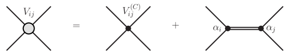
Figure 7: Eq. (A.9) in terms of Feynman Diagrams

In what follows, we give explicit formulae for the contact kernels from the chiral Lagrangians in eq. (A.3) for the different isospin channels. We also give the couplings $\alpha_{i}$ for each scalar resonance. For $I=0$ we include the superscript $(8)$ or $(1)$ in $\alpha_{i}$ to distinguish between the octet and singlet contributions, respectively. For the rest of isospins there is no singlet contribution.

• $I=0$

  $$V_{\pi\pi\to\pi\pi}^{(C)} = \frac{2s-m_{\pi}^{2}}{2f_{\pi}^{2}}$$

  $$V_{\pi\pi\to K\bar{K}}^{(C)} = \frac{\sqrt{3}}{4}\frac{s}{f_{\pi}^{2}}$$

  $$V_{\pi\pi\to\eta\eta}^{(C)} = -\frac{1}{\sqrt{3}}\frac{m_{\pi}^{2}}{f_{\pi}^{2}}$$

  $$V_{K\bar{K}\to K\bar{K}}^{(C)} = \frac{3}{4}\frac{s}{f_{\pi}^{2}}$$

  $$V_{K\bar{K}\to\eta\eta}^{(C)} = -\frac{2}{9}\frac{3s-2m_{\eta}^{2}-m_{K}^{2}}{f_{\pi}^{2}}$$

  $$V_{\eta\eta\to\eta\eta}^{(C)} = \frac{2m_{K}^{2}+m_{\pi}^{2}}{9f_{\pi}^{2}}$$ (A.10)

  $$\alpha^{(8)}_{\pi\pi} = \frac{c_{d}s+2(c_{m}-c_{d})m_{\pi}^{2}}{f_{\pi}^{2}}$$

  $$\alpha^{(8)}_{K\bar{K}} = -\frac{c_{d}s+2(c_{m}-c_{d})m_{K}^{2}}{\sqrt{3}f_{\pi}^{2}}$$

  $$\alpha^{(8)}_{\eta\eta} = \frac{8c_{m}(m_{K}^{2}-m_{\pi}^{2})}{3\sqrt{3}f_{\pi}^{2}}$$ (A.11)

  $$\alpha^{(1)}_{\pi\pi} = \sqrt{6}\frac{\tilde{c}_{d}s+2(\tilde{c}_{m}-\tilde{c}_{d})m_{\pi}^{2}}{f_{\pi}^{2}}$$

  $$\alpha^{(1)}_{K\bar{K}} = -\frac{\tilde{c}_{d}s+2(\tilde{c}_{m}-\tilde{c}_{d})m_{K}^{2}}{2\sqrt{2}f_{\pi}^{2}}$$

  $$\alpha^{(1)}_{\eta\eta} = \sqrt{2}\frac{3\tilde{c}_{d}(s-2m_{\eta}^{2})+2\tilde{c}_{m}(2m_{K}^{2}+m_{\pi}^{2})}{3f_{\pi}^{2}}$$ (A.12)

• $I=1/2$

  $$V_{K\pi\to K\pi}^{(C)} = \frac{s-3u+2m_{K}^{2}+2m_{\pi}^{2}}{4f_{\pi}^{2}}$$

  $$V_{K\pi\to K\eta}^{(C)} = \frac{\sqrt{2}}{6}\frac{3t-m_{\eta}^{2}-2m_{K}^{2}}{f_{\pi}^{2}}$$

  $$V_{K\pi\to K\eta^{\prime}}^{(C)} = -\frac{1}{12}\frac{3t-8m_{K}^{2}-m_{\eta^{\prime}}^{2}-3m_{\pi}^{2}}{f_{\pi}^{2}}$$

  $$V_{K\eta\to K\eta}^{(C)} = \frac{6t-4m_{\eta}^{2}-2m_{K}^{2}}{9f_{\pi}^{2}}$$

  $$V_{K\eta\to K\eta^{\prime}}^{(C)} = -\frac{1}{9\sqrt{2}}\frac{3t-m_{\eta}^{2}-m_{\eta^{\prime}}^{2}-3m_{\pi}^{2}+2m_{K}^{2}}{f_{\pi}^{2}}$$

  $$V_{K\eta^{\prime}\to K\eta^{\prime}}^{(C)} = \frac{1}{36}\frac{3t-2m_{\eta^{\prime}}^{2}+32m_{K}^{2}-6m_{\pi}^{2}}{f_{\pi}^{2}}$$ (A.13)

  $$\alpha_{K\pi} = -\sqrt{\frac{3}{2}}\frac{c_{d}s+(c_{m}-c_{d})(m_{\pi}^{2}+m_{K}^{2})}{f_{\pi}^{2}}$$

  $$\alpha_{K\eta} = -\frac{2}{\sqrt{3}}\frac{c_{m}(m_{K}^{2}-m_{\pi}^{2})}{f_{\pi}^{2}}$$

  $$\alpha_{K\eta^{\prime}} = -\sqrt{\frac{3}{2}}\frac{c_{d}s-c_{d}(m_{K}^{2}+m_{\eta^{\prime}}^{2})-\frac{1}{3}c_{m}(m_{\pi}^{2}-7m_{K}^{2})}{f_{\pi}^{2}}$$ (A.14)

• $I=1$

  $$V_{\pi\eta\to\pi\eta}^{(C)} = \frac{2}{3}\frac{m_{\pi}^{2}}{f_{\pi}^{2}}$$

  $$V_{\pi\eta\to K\bar{K}}^{(C)} = -\frac{3s-2m_{K}^{2}-m_{\eta}^{2}}{3\sqrt{3}f_{\pi}^{2}}$$

  $$V_{\pi\eta\to\pi\eta^{\prime}}^{(C)} = \frac{\sqrt{2}}{3}\frac{m_{\pi}^{2}}{f_{\pi}^{2}}$$

  $$V_{K\bar{K}\to K\bar{K}}^{(C)} = -\frac{u-2m_{\pi}^{2}}{2f_{\pi}^{2}}$$

  $$V_{K\bar{K}\to\pi\eta^{\prime}}^{(C)} = \frac{3s-8m_{K}^{2}-m_{\eta^{\prime}}^{2}-3m_{\pi}^{2}}{6\sqrt{6}f_{\pi}^{2}}$$

  $$V_{K\eta^{\prime}\to K\eta^{\prime}}^{(C)} = \frac{1}{3}\frac{m_{\pi}^{2}}{f_{\pi}^{2}}$$ (A.15)

  $$\alpha_{\pi\eta} = -\frac{2}{\sqrt{3}}\frac{c_{d}s-c_{d}(m_{\pi}^{2}+m_{\eta}^{2})+2c_{m}m_{\pi}^{2}}{f_{\pi}^{2}}$$

  $$\alpha_{K\bar{K}} = \frac{c_{d}s-2(c_{d}-c_{m})m_{K}^{2}}{f_{\pi}^{2}}$$

  $$\alpha_{\pi\eta^{\prime}} = -\frac{2}{\sqrt{6}}\frac{c_{d}s-c_{d}(m_{\pi}^{2}+m_{\eta^{\prime}}^{2})+2c_{m}m_{\pi}^{2}}{f_{\pi}^{2}}$$

• $I=3/2$

  $$V_{K\pi\to K\pi}=-\frac{s-m_{K}^{2}-m_{\pi}^{2}}{2f_{\pi}^{2}}$$ (A.17)

Figure 8: Experimental data and our fits, as explained in the text.

With the amplitudes calculated for meson–meson scattering, we perform several fits, e.g. by changing the value of the highest $\sqrt{s}$ fitted from 1.2 to 1.4 GeV and by imposing that several subtraction constants for the pseudoscalar–pseudoscalar channels are equal, so that we can calculate the pseudoscalar–scalar kernels with different inputs, and then check the independence of our results. We only show our main fit since all the other fits that we obtained give rise to similar results that would not change our conclusions. In this fit the highest value of $\sqrt{s}$ considered is 1.4 GeV. For the octet of scalar resonances we take the values of the parameters $c_{d}$, $c_{m}$ and $M_{8}$ from ref. [60], where $M_{8}$, the mass of this octet, is around 1.3-1.4 GeV. For definiteness, $c_{d}=c_{m}=22.8$ MeV and $M_{8}=1.4$ GeV. The parameters for the singlet resonance exchange, $\widetilde{c}_{d}$, $\widetilde{c}_{m}$ and $M_{1}$ are left free, with the latter the mass of the singlet scalar resonance. Regarding the subtraction constants in the unitarity loop function of the different channels [13] (they play the analogous role of $a_{1}$ in eq. (2.12) but for pseudoscalar-pseudoscalar scattering), we take the most general situation compatible with isospin symmetry. Adopting the same argument as in the appendix A of ref. [62] from SU(3) to SU(2), the subtraction constants corresponding to the same pair of pseudoscalars should be the same in the different isospin. In this way, the subtraction constant for $K\bar{K}$ both in $I=0$ and $I=1$ is taken with the same value. On the other hand, for a given isospin, we also put constraints on the subtraction constants associated with non-relevant channels. In this way, the $K\eta$ subtraction constant in $I=1/2$ is kept equal to that of $K\pi$ and, similarly, for $I=1$ the $\pi\eta^{\prime}$ subtraction constant is put equal to that of $\pi\eta$. Of course, we have checked that smoothing these constraints does not affect the results of the fit. In this way, we finally have six independent subtraction constants for $\pi\pi$, $K\bar{K}$, $\eta\eta$, $K\pi$, $K\eta^{\prime}$ and $\pi\eta$. There is also a normalization constant for the data on an unnormalized $\pi\eta$ event distribution around the $a_{0}(980)$ resonance that is required for each fit. The results of the fit compared to experimental data are shown by the solid line in Fig. 8 and the values of the fitted parameters are given in Table 2.

Parameter	Value
$\tilde{c}_{d}$ (MeV)	$18\pm 1$
$\tilde{c}_{m}$ (MeV)	$23\pm 4$
$M_{1}$ (MeV)	$1100\pm 20$
$a_{\pi\pi}$	$-0.98\pm 0.10$
$a_{K\bar{K}}$	$-1.00\pm 0.20$
$a_{\eta\eta}$	$+0.04\pm 0.22$
$a_{K\pi}$	$+0.17\pm 0.05$
$a_{K\eta^{\prime}}$	$-3.53\pm 0.13$
$a_{\pi\eta}$	$-2.55\pm 0.37$

Table 2: Fitted parameters for the main fit. The $\chi^{2}/\textrm{d.o.f.}$ is $0.96$. The fits are obtained employing the program MINUIT [63].

Resonance	$\textrm{Re}\sqrt{s}\textrm{ (MeV)}$	$\textrm{Im}\sqrt{s}\textrm{ (MeV)}$
$\sigma$	$466$	$235$
$\kappa$	$698$	$294$
$f_{0}(980)$	$987$	$18$
$a_{0}(980)$	$1019$	$33$

Table 3: The pole positions of the scalar resonances obtained from the main fit are given.

Resonance	$g_{K\bar{K}}\textrm{ (GeV)}$	$\left\lvert g_{K\bar{K}}\textrm{ (GeV)}\right\rvert$
$f_{0}(980)$	$-3.72+1.18i$	$3.90$
$a_{0}(980)$	$-4.11+1.59i$	$4.41$

Table 4: Couplings of the $f_{0}(980)$ and $a_{0}(980)$ resonances to $K\bar{K}$ (with definite isospin). These couplings are calculated from the residues of the corresponding pole, see e.g.[13, 64].

The set of experimental data included in the fits for $I=0$ comprises the elastic $\pi\pi$ phase shifts, $\delta_{\pi\pi\to\pi\pi}$, from refs. [65, 66, 67, 68, 69, 70], the phase shift for $\pi\pi\to K\bar{K}$, $\delta_{\pi\pi\to K\bar{K}}$, and $(1-\eta^{2})/4$ from refs. [71, 72], where $\eta$ is the elastic parameter for the $\pi\pi\to\pi\pi$ $I=0$ S-wave. With respect to $I=1/2$ we fit the elastic $\pi K$ phase shifts, $\delta_{K\pi\to K\pi}$, from refs. [73, 74, 75, 76]. Finally, we include an event distribution of $\pi\eta$ around the $a_{0}(980)$ resonance mass from the central production of $\pi\pi\eta$, ref. [77], fitted like in ref. [11, 12].

Once the fits are performed we look for the poles of the scalar resonances $\sigma$, $\kappa$, $f_{0}(980)$ and $a_{0}(980)$ in the unphysical Riemann sheets continuously connected with the physical one. Notice that only the $f_{0}(980)$ and $a_{0}(980)$ poles are actually required for evaluating the pseudoscalar–scalar scattering kernels in section 2. The $\sigma$ and $\kappa$ are given for completeness. They are related to the $f_{0}(980)$ and $a_{0}(980)$ resonances giving rise to a nonet of light scalar resonances [44]. Other poles around 1.4 GeV also appear that we do not include here. The pole positions are given in Table 3. The couplings of the $f_{0}(980)$ and $a_{0}(980)$ to $K\bar{K}$, used in this work, are collected in Table 4.

Appendix B S-wave projection of $C_{3}$ and $C_{4}(M_{4}^{2})$

The three- and four-point Green functions $C_{3}$ and $C_{4}(m_{4}^{2})$ are defined in eq. (2.5). Here, we consider the more general case with arbitrary internal masses and from the very beginning the S-wave projection is worked out. Both functions are finite.

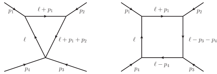
Figure 9: Feynman diagrams for $C_{3}$ (left) and $C_{4}(m_{4}^{2})$ (right).

We first consider $C_{3}$, left diagram of Fig. 9, and follow its notation with $t=(p_{1}+p_{2})^{2}$ (note that all four-momenta are in-going). We also introduce two Feynman parameters $u_{1}$ and $u_{2}$ and the relative angle $\theta$ between the initial and final pseudoscalars, so that

$$C_{3} =\frac{i}{2}\int_{-1}^{+1}d\cos\theta\int\frac{d^{4}\ell}{(2\pi)^{4}}\frac{1}{((\ell+p_{1})^{2}-m_{1}^{2})(\ell^{2}-m_{2}^{2})((\ell+p_{1}+p_{2})^{2}-m_{3}^{2})}$$

$$=\frac{1}{32\pi^{2}}\int_{0}^{1}du_{1}\int_{0}^{u_{1}}du_{2}\int_{-1}^{+1}d\cos\theta\left[p_{2}^{2}u_{1}^{2}+p_{1}^{2}u_{2}^{2}+2p_{1}p_{2}u_{1}u_{2}\right.$$

$$\left.+(m_{1}^{2}-m_{3}^{2}-p_{2}^{2})u_{1}+(m_{2}^{2}-m_{1}^{2}-p_{1}^{2}-2p_{1}p_{2})u_{2}+m_{3}^{2}+i\varepsilon\right]^{-1}~{}.$$ (B.1)

Then, $\cos\theta$ is introduced by taking into account that $p_{1}p_{2}=(t-p_{1}^{2}-p_{2}^{2})/2$ with $t=q_{0}^{2}-|\mathbf{p}|^{2}-|\mathbf{p}^{\prime}|^{2}+2|\mathbf{p}||\mathbf{p}^{\prime}|\cos\theta$, with $q^{0}=p_{1}^{0}-p_{2}^{0}$, the difference of energies between the initial and final scalar resonances. We perform the angular integration and introduce the parameter $\xi_{2}$ as $u_{2}=u_{1}\xi_{2}$, so that

$$C_{3} =\frac{1}{64\pi^{2}|\mathbf{p}||\mathbf{p}^{\prime}|}\int_{0}^{1}\frac{du_{1}}{1-u_{1}}\int_{0}^{1}\frac{d\xi_{2}}{\xi_{2}}\left[\log(1+\psi)-\log(-1+\psi)\right]~{},$$ (B.2)

where

$$\psi =\frac{1}{2|\mathbf{p}||\mathbf{p}^{\prime}|(1-u_{1})u_{2}}\left[p_{2}^{2}u_{1}^{2}+p_{1}^{2}u_{2}^{2}+u_{1}u_{2}(q_{0}^{2}-|\mathbf{p}|^{2}-|\mathbf{p}^{\prime}|^{2}-p_{1}^{2}-p_{2}^{2})\right.$$

$$\left.+u_{1}(m_{1}^{2}-m_{3}^{2}-p_{2}^{2})+u_{2}(m_{2}^{2}-m_{1}^{2}+p_{2}^{2}-q_{0}^{2}+|\mathbf{p}|^{2}+|\mathbf{p}^{\prime}|^{2})+m_{3}^{2}-i\varepsilon\right]^{-1}~{}.$$ (B.3)

For the four-point function $C_{4}(m_{4}^{2})$, right diagram of Fig. 9, one has

$$C_{4}(m_{4}^{2}) =\frac{i}{2}\int_{-1}^{+1}d\cos\theta\int\frac{d^{4}\ell}{(2\pi)^{4}}\frac{1}{((\ell+p_{1})^{2}-m_{1}^{2})(\ell^{2}-m_{2}^{2})}$$

$$\times\frac{1}{((\ell-p_{3}-p_{4})^{2}-m_{3}^{2})((\ell-p_{4})^{2}-m_{4}^{2})}~{}.$$ (B.4)

In this case there is no ambiguity if instead of performing the $\cos\theta$ integration one directly calculates the related integration over $t=(p_{3}+p_{4})^{2}$ by taking into account that $dt=2|\mathbf{p}||\mathbf{p}^{\prime}|d\cos\theta$ (ambiguities could arise for $s$ such that the product $|\mathbf{p}||\mathbf{p}^{\prime}|$ becomes complex. The particular integration to be performed here is not affected by such problem, see below.) We also introduce three Feynman parameters $u_{1}$, $u_{2}$ and $u_{3}$ so that

$$C_{4}(m_{4}^{2}) =\frac{-1}{64\pi^{2}|\mathbf{p}||\mathbf{p}^{\prime}|}\int_{0}^{1}du_{1}\int_{0}^{u_{1}}du_{2}\int_{0}^{u_{2}}du_{3}\int_{t_{-}}^{t_{+}}dt\left[p_{1}^{2}(1-u_{2}+u_{3})(u_{2}-u_{3})\right.$$

$$\left.+2p_{1}p_{3}(u_{1}-u_{2})(u_{2}-u_{3})+2p_{1}p_{4}(1-u_{2})(u_{2}-u_{3})-m_{2}^{2}u_{3}\right.$$

$$\left.+p_{3}^{2}(1-u_{1}+u_{2})(u_{1}-u_{2})+2p_{3}p_{4}(u_{1}-u_{2})u_{2}+p_{4}^{2}(1-u_{2})u_{2}\right.$$

$$\left.-m_{1}^{2}(u_{2}-u_{3})-m_{3}^{2}(u_{1}-u_{2})-m_{4}^{2}(1-u_{1})-i\varepsilon\right]^{-1}~{}.$$ (B.5)

In terms of the variable $t$ the previous integral is of the from $\int dt/(at+b)^{2}$ so that the $t$-integration can be done straightforwardly without problems in its analytical extrapolation. The resulting $u_{3}$-integration is of the form $\int du_{3}/[u_{3}(u_{3}^{2}+\beta u_{3}+\gamma)]$ that can also be done straightforwardly by factorizing the second-order polynomial in the denominator. Our final expression for $C_{4}(m_{4}^{2})$ is

$$C_{4}(m_{4}^{2})=\frac{-1}{64p_{1}^{2}|\mathbf{p}||\mathbf{p}^{\prime}|}\int_{0}^{1}du_{1}\int_{0}^{1}\frac{d\xi_{2}}{1-\xi_{2}} \left[\psi(t_{+},u_{2})-\psi(t_{+},0)\right.$$

$$\left.-\psi(t_{-},u_{2})+\psi(t_{-},0)\right]~{},$$ (B.6)

where

$$\psi(t,u_{3}) =\frac{\log u_{3}}{y_{1}y_{2}}+\frac{\log(u_{3}-y_{1})}{y_{1}(y_{1}-y_{2})}-\frac{\log(u_{3}-y_{2})}{y_{2}(y_{1}-y_{2})}~{},$$

$$u_{3}^{2}+\beta u_{3}+\gamma =(u_{3}-y_{1})(u_{3}-y_{2})~{},$$

$$p_{1}^{2}(u_{3}^{2}+\beta u_{3}+\gamma) =m_{4}^{2}(1-u_{1})+m_{3}^{2}(u_{1}-u_{2})+p_{3}^{2}(-1+u_{1})(u_{1}-u_{2})+m_{1}^{2}u_{2}$$

$$+u_{2}(s(-1+u_{1})+p_{2}^{2}(u_{2}-u_{1}))-(m_{1}^{2}-m_{2}^{2}+p_{4}^{2})u_{3}+p_{1}^{2}u_{3}^{2}$$

$$+(s(1-u_{1})+(p_{2}^{2}+p_{4}^{2}-t)u_{1}-(p_{1}^{2}+p_{2}^{2}-t)u_{2})u_{3}-i\varepsilon~{},$$

$$t_{\pm} =(p_{3}^{0}-p_{4}^{0})^{2}-(|\mathbf{p}|\mp|\mathbf{p}^{\prime}|)^{2}~{}.$$ (B.7)

The S-wave projection of the three- and four-point functions $C_{3}$ and $C_{4}(m_{4}^{2})$ was also obtained for some kinematical regions and values of $m_{4}^{2}$ from ref. [78], wherever the latter could be applied. In such cases our results and ref. [78] agree.

References

• [1] Y. Nambu, Phys. Rev. Lett.  4, 380 (1960).
• [2] M. Gell-Mann, Phys. Rev.  125, 1067 (1962).
• [3] S. L. Glashow and S. Weinberg, Phys. Rev. Lett.  20, 224 (1968).
• [4] S. R. Coleman and E. Witten, Phys. Rev. Lett.  45 (1980) 100.
• [5] S. Weinberg, Phys. Rev. Lett.  17, 616 (1966).
• [6] S. Weinberg, Physica A 96, 327 (1979).
• [7] J. Gasser and H. Leutwyler, Annals Phys.  158 (1984) 142.
• [8] J. Gasser and H. Leutwyler, Nucl. Phys.  B 250 (1985) 465.
• [9] J. A. Oller and E. Oset, Nucl. Phys.  A 620, 438 (1997); (E)-ibid.  A 652, 407 (1999).
• [10] A. Dobado and J. R. Pelaez, Phys. Rev.  D 47, 4883 (1993).
• [11] J. A. Oller, E. Oset and J. R. Pelaez, Phys. Rev. Lett.  80 (1998) 3452.
• [12] J. A. Oller, E. Oset and J. R. Pelaez, Phys. Rev.  D 59 (1999) 074001; (E)-ibid D 60 (1999) 099906; (E)-ibid D 75 (2007) 099903.
• [13] J. A. Oller and E. Oset, Phys. Rev.  D 60 (1999) 074023.
• [14] C. Amsler et al. (Particle Data Group), Physics Letters B 667 (2008) 1.
• [15] T. Barnes, F. E. Close, P. R. Page and E. S. Swanson, Phys. Rev.  D 55 (1997) 4157.
• [16] E. Klempt and A. Zaitsev, Phys. Rept.  454, 1 (2007).
• [17] F. E. Close and P. R. Page, Nucl. Phys.  B 443 (1995) 233; Phys. Rev.  D 52 (1995) 1706.
• [18] A. Masoni, C. Cicalo and G. L. Usai, J. Phys. G 32 (2006) R293.
• [19] C. Amsler et al. [Crystal Barrel Collaboration], Phys. Lett.  B 358 (1995) 389; A. Abele et al. [Crystal Barrel Collaboration], Nucl. Phys.  B 514 (1998) 45.
• [20] A. Bertin et al. [OBELIX Collaboration], Phys. Lett.  B 361 (1995) 187; C. Cicalo et al. [OBELIX Collaboration], Phys. Lett.  B 462 (1999) 453.
• [21] Z. Bai et al. [MARK-III Collaboration], Phys. Rev. Lett.  65 (1990) 2507.
• [22] J. E. Augustin et al. [DM2 Collaboration], Phys. Rev.  D 46 (1992) 1951.
• [23] M. Acciarri et al. [L3 Collaboration], Phys. Lett.  B 501 (2001) 1.
• [24] M. Chanowitz, Phys. Rev. Lett. 46 (1981) 981; K. Ishikawa, ibid. 46 (1981) 978.
• [25] F. E. Close, G. R. Farrar and Z. p. Li, Phys. Rev.  D 55 (1997) 5749.
• [26] G. S. Bali, K. Schilling, A. Hulsebos, A. C. Irving, C. Michael and P. W. Stephenson [UKQCD Collaboration], Phys. Lett.  B 309 (1993) 378.
• [27] C. J. Morningstar and M. J. Peardon, Phys. Rev.  D 60 (1999) 034509.
• [28] Y. Chen et al., Phys. Rev.  D 73 (2006) 014516.
• [29] M. Albaladejo and J. A. Oller, Phys. Rev. Lett.  101 (2008) 252002.
• [30] M. Chanowitz, Phys. Rev. Lett.  95 (2005) 172001; Phys. Rev. Lett.  98 (2007) 149104.
• [31] S. Narison, Nucl. Phys.  B 509 (1998) 312.
• [32] L. Faddeev, A. J. Niemi and U. Wiedner, Phys. Rev.  D 70 (2004) 114033.
• [33] G. R. Farrar, Phys. Rev. Lett. 76 (1996) 4111.
• [34] M. B. Cakir and G. R. Farrar, Phys. Rev.  D 50 (1994) 3268.
• [35] E. Klempt, “The glueball candidate $\eta(1440)$ as $\eta$ radial excitation.” Thirty-second International Conference on High-Energy Physics (ICHEP04), Beijing, China, arXiv:hep-ph/0409148.
• [36] J. Z. Bai et al. [BES Collaboration], Phys. Rev. Lett. 91 (2003) 022001.
• [37] M. Ablikim et al. [BES Collaboration], Phys. Rev. Lett.  95 (2005) 262001.
• [38] A. Sibirtsev, J. Haidenbauer, S. Krewald, U. G. Meissner and A. W. Thomas, Phys. Rev.  D 71 (2005) 054010; J. Haidenbauer, U. G. Meissner and A. Sibirtsev, Phys. Rev.  D 74 (2006) 017501; Phys. Lett.  B 666 (2008) 352.
• [39] L. Alvarez-Ruso, J. A. Oller and J. M. Alarcon, Phys. Rev.  D 80 (2009) 054011.
• [40] L. Alvarez-Ruso, J. A. Oller and J. M. Alarcon, arXiv:1007.4512 [hep-ph].
• [41] B. Aubert et al. [BABAR Collaboration], Phys. Rev.  D 74 (2006) 091103; Phys. Rev.  D 76 (2007) 012008.
• [42] C. P. Shen et al. [Belle Collaboration], Phys. Rev.  D 80 (2009) 031101.
• [43] A. Martinez Torres, K. P. Khemchandani, L. S. Geng, M. Napsuciale and E. Oset, Phys. Rev.  D 78 (2008) 074031.
• [44] J. A. Oller, Nucl. Phys.  A 727 (2003) 353 [arXiv:hep-ph/0306031].
• [45] G. Janssen, B. C. Pearce, K. Holinde and J. Speth, Phys. Rev.  D 52 (1995) 2690.
• [46] J. D. Weinstein and N. Isgur, Phys. Rev. Lett.  48 (1982) 659; Phys. Rev.  D 41 (1990) 2236.
• [47] J. A. Oller and L. Roca, Eur. Phys. J.  A 34 (2007) 371 [arXiv:hep-ph/0608290].
• [48] G. F. Chew and S. Mandelstam, Phys. Rev.  119 (1960) 467.
• [49] J. A. Oller and U. G. Meissner, Phys. Lett.  B 500 (2001) 263.
• [50] G. Barton, “Introduction to Dispersion Techniques in Field Theory”, W. A. Benjamin, Inc, New York, Amsterdam, 1965.
• [51] A. M. Bincer, Phys. Rev. 118 (1960) 855.
• [52] G. Källen and A. S. Wightman, Mat. Fys. Skr. Dan. Vid. Selsk. 1 no. 6, (1958) 1.
• [53] C. Daum et al. [ACCMOR Collaboration], Nucl. Phys.  B 187 (1981) 1.
• [54] G. W. Brandenburg et al., Phys. Rev. Lett.  36 (1976) 1239.
• [55] R. S. Longacre, Phys. Rev.  D 42 (1990) 874.
• [56] S. Fukui et al., Phys. Lett.  B 267 (1991) 293.
• [57] E. Witten, Nucl. Phys.  B 223 (1983) 422.
• [58] P. Herrera-Siklody, J. I. Latorre, P. Pascual and J. Taron, Nucl. Phys.  B 497 (1997) 345.
• [59] R. Kaiser and H. Leutwyler, Eur. Phys. J.  C 17 (2000) 623.
• [60] M. Jamin, J. A. Oller and A. Pich, Nucl. Phys.  B 587 (2000) 331.
• [61] G. Ecker, J. Gasser, A. Pich and E. de Rafael, Nucl. Phys.  B 321, 311 (1989).
• [62] D. Jido, J. A. Oller, E. Oset, A. Ramos and U. G. Meissner, Nucl. Phys.  A 725 (2003) 181.
• [63] F. James, Minuit Reference Manual D 506 (1994).
• [64] K. L. Au, D. Morgan and M. R. Pennington, Phys. Rev.  D 35 (1987) 1633.
• [65] G. Grayer et al., Proc. 3rd Philadelphia Conf. on Experimental Meson Spectroscopy, Philadelphia, 1972 (American Institute of Physics, New York, 1972) p. 5.
• [66] P. Estabrooks et al., AIP Conf. Proc. 13 (1973) 37.
• [67] R. Kaminski, L. Lesniak and K. Rybicki, Z. Phys.  C 74, 79 (1997) [arXiv:hep-ph/9606362].
• [68] C. D. Froggatt and J. L. Petersen, Nucl. Phys.  B 129, 89 (1977).
• [69] B. Hyams et al., Nucl. Phys.  B 64, 134 (1973) [AIP Conf. Proc.  13, 206 (1973)].
• [70] S. D. Protopopescu et al., Phys. Rev.  D 7, 1279 (1973).
• [71] D. H. Cohen, D. S. Ayres, R. Diebold, S. L. Kramer, A. J. Pawlicki and A. B. Wicklund, Phys. Rev.  D 22, 2595 (1980).
• [72] A. Etkin et al., Phys. Rev.  D 25, 1786 (1982).
• [73] R. Mercer et al., Nucl. Phys.  32B, 381 (1971).
• [74] P. Estabrooks, R. K. Carnegie, A. D. Martin, W. M. Dunwoodie, T. A. Lasinski and D. W. G. Leith, Nucl. Phys.  B 133, 490 (1978).
• [75] H. H. Bingham et al., Nucl. Phys.  B 41, 1 (1972).
• [76] D. Aston et al., Nucl. Phys.  B 296, 493 (1988).
• [77] T. A. Armstrong et al. [WA76 Collaboration and Athens-Bari- Birmingham-CERN-College de France Collab], Z. Phys.  C 52, 389 (1991).
• [78] A. van Hameren, C. G. Papadopoulos and R. Pittau, JHEP 0909 (2009) 106.