Young Stellar Groups and Their Most Massive Stars

Abstract

We analyze the masses and spatial distributions of fourteen young stellar groups in Taurus, Lupus3, ChaI, and IC348. These nearby groups, which typically contain 20 to 40 members, have membership catalogs complete to $\sim$0.02 M_⊙, and are sufficiently young that their locations should be similar to where they formed. These groups show five properties seen in clusters having many more stars and much greater surface density of stars: (1) a broad range of masses, (2) a concentration of the most massive star towards the centre of the group, (3) an association of the most massive star with a high surface density of lower-mass stars, (4) a correlation of the mass of the most massive star with the total mass of the group, and (5) the distribution of a large fraction of the mass in a small fraction of the stars.

1 INTRODUCTION

Most stars are believed to form in clusters (Lada & Lada, 2003), and clusters also harbour most, if not all, massive stars (e.g, Zinnecker & Yorke, 2007). The nearest star-forming regions within a few hundred pc, however, have few clusters according to most definitions (Reipurth, 2008). There, low mass stars form primarily in an “isolated” mode, and high mass stars are absent.

There has been relatively little work investigating the transition between these two regimes. Several authors have considered this transition from the perspective of a continuum of clustering, rather than two discrete states. Elmegreen (2008), for example, theoretically examined which physical conditions within a turbulent molecular complex lead to the formation of bound clusters versus more dispersed stellar systems. Varied physical conditions could account for the substantial variations in properties of young massive star-forming regions seen in nearby galaxies (Maíz-Apellániz, 2001), as well as the presence or absence of clusters within portions of the local Gould Belt structure (Elias, Alfaro, & Cabrera-Caño, 2009). Within the nearest few hundred parsecs, Bressert et al (2010) recently demonstrated that there is no evidence for a preferred length-scale for clustering of YSOs detected with Spitzer.

Despite this evidence that there may not be a sharp boundary between clustered and isolated modes of star-formation, there are distinctions between the two at least in terms of processes that will influence later evolution (discussed in Section 5.1). In such a manner, the transition between the regime where processes associated with clusters are important, and the regime where they are not is expected to occur for stellar groupings whose most massive member is between roughly 2 and 15 M_⊙ (Testi et al, 1999). In this transition range, do stellar groups exhibit properties typical of clusters (e.g., mass segregation and high surface density of sources), or are their properties more similar to those of isolated star formation?

Testi et al (1999, and references therein) observed 44 Herbig Ae/Be stars and their surroundings in order to study this transition. They focussed on cluster richness indicators (number and surface density of cluster members) around each star targeted. They found that both measures tend to decrease from early to late B spectral types, and then show relatively little trend through the A spectral types, although there is large scatter at all spectral types. A significant fraction of the late-Be and Ae stars show little evidence for belonging to a group or cluster. Massi, Lorenzetti & Giannini (2003) find a similar result in the Vela C and D clouds, using the bolometric luminosity, $L_{bol}$, as a proxy for mass in these young star-forming regions. They found all IRAS sources with L_bol $\gtrsim 10^{3}L_{\odot}$ and some lower $L_{bol}$ sources show evidence of clustering.

In this paper, we examine this transition further, focussing on the properties of the most massive member or members of each group. With sensitive near-IR data from Spitzer, in combination with large ground-based spectral surveys, catalogs of YSOs with excellent completeness are now available for several nearby star-forming regions. These catalogs allow us to analyze the properties of stellar groupings in the transition range in ways not possible for the more distant regions studied in Testi et al (1999) and Massi, Lorenzetti & Giannini (2003), since the nearby regions considered here have deeper and more uniform completeness levels.

Our main conclusions are that within the groups we identify, similar to clusters, the members have a broad range in masses, with a significant fraction of the mass being found within the few most massive members, consistent with an IMF-like distribution. Within each group, the most massive member is centrally-located, and is in or near a region of enhanced source density. We find a correlation between the mass of the most massive member and the total mass of the group similar to that found in larger clusters.

In Section 2, we describe the YSO catalogs we use in our analysis, with further detail in Appendices A and B, while our procedure for identifying groups of YSOs is discussed in Section 3. We analyze the properties of the groups identified in Section 4, focussing on mass segregation and clustering, then discuss the implications in Section 5, and conclude in Section 6. Our procedure for estimating the YSO masses and our sources of uncertainty are examined in Appendices C and D.

2 DATA

To analyze the properties of young stellar groups, we require the stars to be nearby (within $\sim$300 pc) to prevent source confusion. We require the stars to be younger than several Myr, so that their natal groups have not had time for significant dynamical evolution. The stars must also be old enough (roughly class I/II or higher) so that accurate spectral types can be determined, and hence reasonable mass estimates made. Finally, the census of stars must be complete to better than 90% to masses below the brown dwarf limit (0.08 M_⊙) in order for us to apply our analysis. Applying these criteria, there are four nearby star-forming regions for which suitable YSO catalogs exist – Taurus, ChaI, Lupus 3 and IC348, all of which include members out to late M (or even L0) spectral types. This sample differs from other samples of nearby star-forming regions such as those listed in Evans et al (2009), Gutermuth et al (2009), and Myers (2009a) largely due to our requirement of spectral classifications. Most of the groups in this sample correspond to previously identified groups, while ChaI 2 and IC348 1 correspond to small clusters, as discussed in Section 3.

The YSO catalogs we analyze do not include the most deeply embedded objects. Most class 0 and some class I sources are likely missing from our catalogs, as discussed further in Appendix A.5. These are estimated to comprise fewer than $\sim$ 7% of the members of any group considered, based on the distribution of classes in Evans et al (2009). Since our analysis focusses on the relationship between the most massive member of each group and the group as a whole, this incompleteness is unlikely to affect our results.

The YSO catalogs for the four nearby star-forming regions are given in Tables 3 through 6 (available online only), which list the position, common name(s), spectral type, estimated mass (see Section 2.1 and Appendix C), and the group each source is associated with in our analysis (see Section 3). Appendix A and B describe the catalogs in more detail.

2.1 Mass Estimation

For each of the YSOs, we estimate the mass based on the spectral type. We assume a constant age of 1 Myr for all YSOs and follow the procedure outlined in Luhman et al (2003), using a combination of models from Palla & Stahler (1999), Baraffe et al (1998), and Chabrier et al (2000) to estimate the masses. The assumption of a constant, 1 Myr age, as well as the exact stellar models chosen, leads to uncertainties in the masses of order 50%. This is discussed in more detail in Appendix C.

2.2 Additional Data – ONC1

In several parts of the following analysis, we compare the results for the four nearby star-forming regions with the large cluster encompassing the Trapezium in the Orion Nebula Cluster, to represent properties typical to young clusters. To make this comparison, we use the ONC1 dataset from Hillenbrand (1997), adopting the masses and positions given there. We include all sources listed as having a 70% or higher probability of membership. This list contains 721 sources, of which we identify 410 of these as belonging to the Trapezium cluster (see Section 3 for our method of identifying groups and clusters). Of these 410 Trapezium cluster sources, 26 do not have estimated masses in Hillenbrand (1997); we assign each of these the median mass in the cluster (0.23 M_⊙).

3 IDENTIFICATION OF GROUPS

Within each of the four regions in our dataset, there are clearly small groupings of YSOs. In order to define these groups, we use the minimal spanning tree (MST) algorithm (Barrow et al, 1985), following the procedure of Gutermuth et al (2009). Many methods can and have been used to identify groups and clusters in various studies; Bressert et al (2010) find that clustering of YSOs in nearby molecular clouds tends to be best described by a continuum, rather than a single discrete value separating clustered versus non-clustered regions. We adopt the MST to define stellar groups, as it can be applied to multiple regions in an easily reproducible manner, does not require unique thresholds to be set a priori, and is independent of the distance to the region; other cluster-identification schemes are discussed in Appendix D. Our analysis is relatively insensitive to the continuum of clustering – inclusion of more or fewer YSOs in each group does not to have a major effect on our results, as discussed in Appendix D.

Minimal spanning trees are structures where all points in a region are connected via the minimum distance between them (i.e., nearest neighbours); each of these connections is a ‘branch’. The MST structure mimics how the eye naturally connect points; most constellations are connected via their MST, for example.

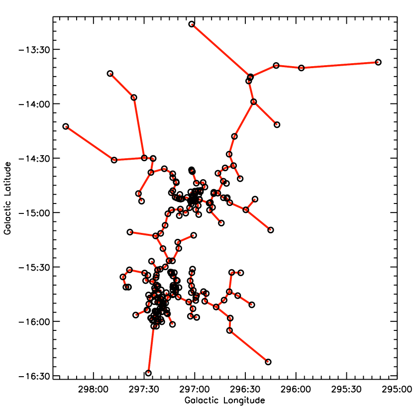
Figure 1: An overview of the YSOs identified in ChaI. The black circles denote the locations of all of the YSOs in the region, while the red lines indicate the MST structure. The left panel shows the entire original MST structure, whereas the right panel shows the MST structure after branches longer than the critical length have been removed, zooming in on on the clustered region of the left panel. The region is plotted in galactic projection for easier comparison with Figure 4. See Section 3 for more details.

The left panel of Figure 1 shows the MST structure in the ChaI region. Groups are apparent within a region by eye as having smaller separations between members than typical in the region as a whole. Within the MST structure, groups can be separated as having “small” branch lengths between all members, i.e., less than some cutoff branch length. Although this length could be defined in an absolute sense, Gutermuth et al (2009) find it more effective to determine a critical length based on the distribution of branch lengths within a given region. This has the advantage of being insensitive to the uncertainty in distance to the region, relying only on the clustering properties of the sources within the region. This method is discussed in more detail in Appendix D.1.

The right panel of Figure 1 shows the resulting groups in ChaI when branches with lengths larger than the critical length are removed. After this ‘pruning’ of the MST, isolated groupings of YSOs remain. These groupings range from very small numbers of sources (e.g., isolated pairs) to larger groups.

For our analysis, we consider only groups which have more than ten members. This cutoff value is somewhat arbitrary, and is based on a visual examination of the groupings identified in Taurus. This examination indicates that groupings of very small numbers of sources would not allow group properties to be examined meaningfully, while a minimum group size of twenty or thirty members would exclude some visually-striking smaller groups.

Using this MST procedure, we identify fourteen groups with more than ten members in our dataset – eight in Taurus, three in ChaI, two in IC348, and one in Lupus3. The four star-forming regions are all much more ‘clustered’ than expected from a random distribution – as a test, we ran our MST algorithm on a set of N_YSO randomly distributed points within each region (where N_YSO is the number of YSOs within each region). When the same critical length scale is adopted as is measured for the observed YSOs, no groupings of more than ten members are found for any of the four regions.

Using the MST procedure, we also identify five groups in the Hillenbrand (1997) ONC1 dataset, representing the main ONC1 cluster (with 410 members) and four additional small groups (typically around 15 members). We compare only the large ONC1 cluster with our groups, as this best represents the properties of a cluster. The smaller groups identified in ONC1 may be affected by incompleteness; the 70% probability of membership criterion we applied may exclude some bona fide members, but this is unlikely to affect our measures in the main ONC1 cluster.

3.1 Groups and Their Environments

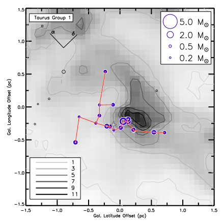
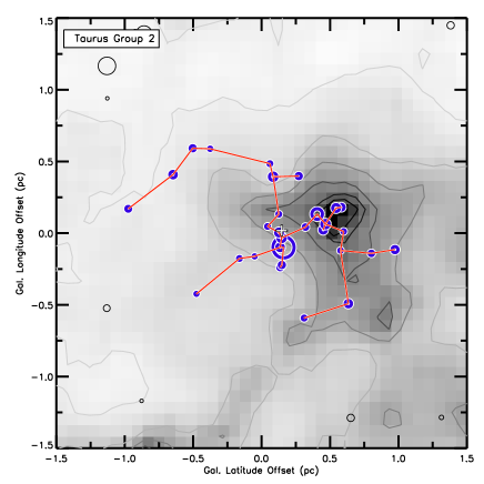
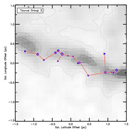
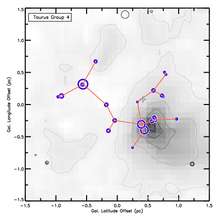
Figure 2: The groups identified using the MST technique in each of the four regions. Groups in Taurus are shown in this figure; the other groups are in the following figures. Blue circles indicate the YSOs within each group, with the circle size scaling linearly with the estimated mass (see first panel for scaling used). Red lines indicate the MST branches in the group. Non-group YSOs in the vicinity are shown in black. The greyscale and contours in the background show the extinction measured. The greyscale ranges from A_V of 15 mag (black) to 0 (white), with contours drawn at 1 to 11 mag (see scale bar in first panel). The orientation of the figures is in galactic co-ordinates to match the native projection of the extinction maps; the first panel shows the direction of increasing RA and dec. All figures are centred on the group’s mid-point position. The median group member position given in Table 1 is indicated by the white plus.

The groups we identify in Taurus, Lupus3, ChaI, and IC348 are shown in Figures 2 through 5, and their properties are summarized in Table 1. In the figures, the group members are indicated by blue circles (with the radius scaling linearly with mass), the red lines denote the MST structure, and the thin black circles denote nearby YSOs that do not belong to the group. The greyscale images in the background indicate the present-day distribution of extinction based on stellar reddening. Displayed are extinction data from Froebrich et al (2007) for Taurus, Dobashi et al (2005) for ChaI, a combination of Teixeira et al. (2005) and Rowles & Froebrich (2009) for Lupus3, and Rowles & Froebrich (2009) for IC348.

As can be seen in Figures 2 through 5, the groups often lie near, but not on, regions of high extinction, suggesting the YSOs have accreted and/or blown away a similar distribution of gas from their immediate environs. In most cases, the mass of gas required to create the present-day stellar masses corresponds to a uniform gas and dust having A${}_{V}\simeq 3$ mag, assuming a formation efficiency of 30%. This extinction due to smoothed-out stellar mass is approximately the difference between the maximum nearby extinction and the mean value of the extinction within the group.

The main group in IC348 is an exception, requiring roughly ten times more material for the formation of the YSOs, which is substantially higher than the present-day nearby extinction. The Lupus3 group also shows a much larger difference in extinction than do most of the other groups, since the high-resolution extinction map from Teixeira et al. (2005) allows much larger peaks in extinction to be measured. At comparable resolutions to the other regions, however, the difference in extinction is similar to that in the other regions. At the same time, the total amount of material remaining in the area spanned by each group is usually insufficient, or barely sufficient, to form a group with mass equal to the mass in the group we observe.

In other words, the immediate areas in which we see the YSOs in the groups appear largely or entirely finished with the star-formation process, but there are still reservoirs of material nearby which are capable of forming a significant number of new stars.

3.2 Comparison with Previously Identified Groups

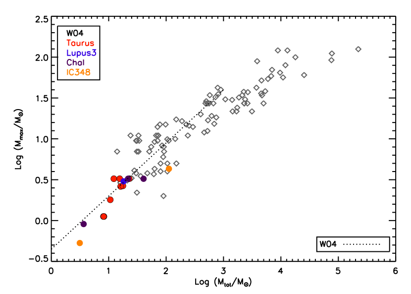
Figure 8: The maximum mass member of each group versus the total mass in the group. The black diamonds represent the data in Weidner et al (2010) (using the new dynamical mass estimates where appropriate), and the dotted line shows approximately the linear tail to the Weidner et al (2010) relationship, assuming a Salpeter slope for the upper end of the IMF. Our groups fit the trend seen in higher mass clusters quite well.

In Taurus, there is good correspondence between the groups we identify and those previously identified using other methods. The Gomez et al (1993) Groups I through VI correspond to our groups 1, 2, 7, 5, 6, and 4 (B209, L1495E, L1527, L1529, L1536, and L1551) respectively, with our remaining two groups (3 / B213 and 8 / L1517) corresponding to un-named contours of higher stellar density in their Figure 8 (right of their Group III and the upper left of the figure respectively). Group I in Jones & Herbig (1979) corresponds roughly to our Groups 1 and 2 (B209 & L1495E), their Group IIa corresponds to our Group 5 (L1529), their surrounding Group II encompasses our Groups 6 and 7 (L1536 & L1527), and their Group III is our Group 4 (L1551). Our Group 3 (B213) lies between their Group II and III with too few stars in their catalog to be classified as a group, and our Group 8 (L1517) lies beyond their catalog.

The main group in IC348 appears most similar to a small cluster, and has been studied in that vein by a variety of authors – see Herbst (2008) and references therein. The two largest groupings of stars in ChaI have also been viewed in a similar manner – see, for example, Luhman (2007).

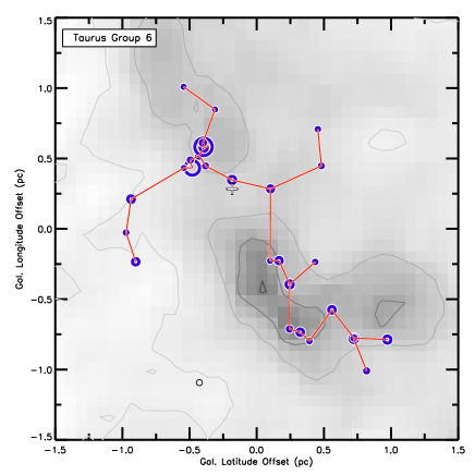
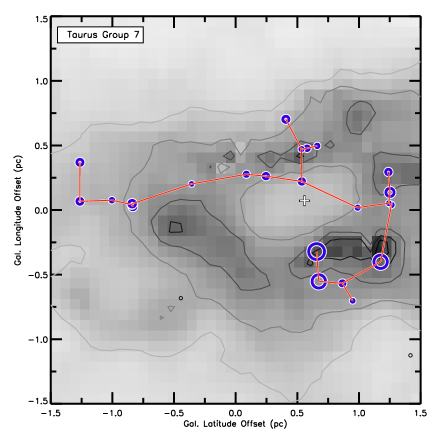
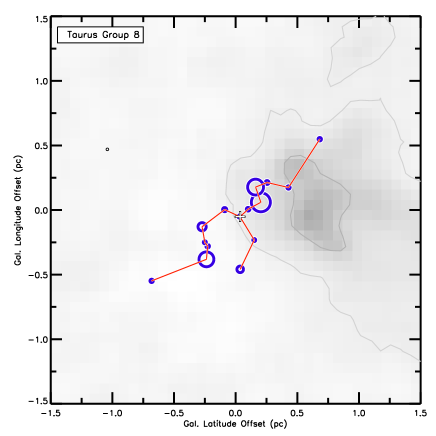
Figure 3: More groups identified in Taurus. See Figure 2 caption for details.

As can be seen from the figures, some of the groups are irregularly shaped, particularly when the total number of members is small. Some groups appear filamentary, such as B213 in Taurus, unlike the conventional picture of a group, which tend to be more circular. Despite these irregularities, we find that the median member position (shown as white plus signs in Figures 2 through 5) is usually a good representation of the apparent centre of the group, although this becomes poorer in the case of the most filamentary groups, as illustrated in Taurus Groups 1 and 2 (Figure 2) versus Taurus Group 6 (Figure 3), for example. The mean member position is sometimes a worse descriptor of the group centre than the median, as it is more likely to be skewed by one or two group members lying preferentially in one direction away from where most of the group is concentrated. The centre of mass tends to lie between the median and mean positions. The centres of the groups as defined by the median positions of the group members are also given in Table 1.

4 RESULTS

4.1 Mass Distribution

Using the masses estimated for each YSO, we examine the distribution of masses within each group. Figure 6 shows the distribution of masses within the main IC348 group. A prominent excess of sources with masses around 2-3 M_⊙ is clearly evident; a similar trend is seen in many of the other groups, although at a much lower level, since the groups are smaller. This excess is unlikely real, and is at least in part caused by our adoption of a single age for all of the stars. Assuming a single age of 2 Myr instead of 1 Myr, for example, reduces the size of the excess (for a given spectral type, assuming an older age will reduce the mass estimated); allowing for an age spread would eliminate it completely (see, e.g., the IC348 mass distribution in Luhman et al, 2003). In order to keep our analysis simple, we maintain our assumption of a single age, recognizing that the details of the mass distributions in the groups are affected by this assumption. For our analysis, however, the detailed mass distribution is not important; we are concerned primarily with the rank of the masses (Sections 4.2-4.4), which is determined solely by the spectral type, as well as other broad properties (this section).

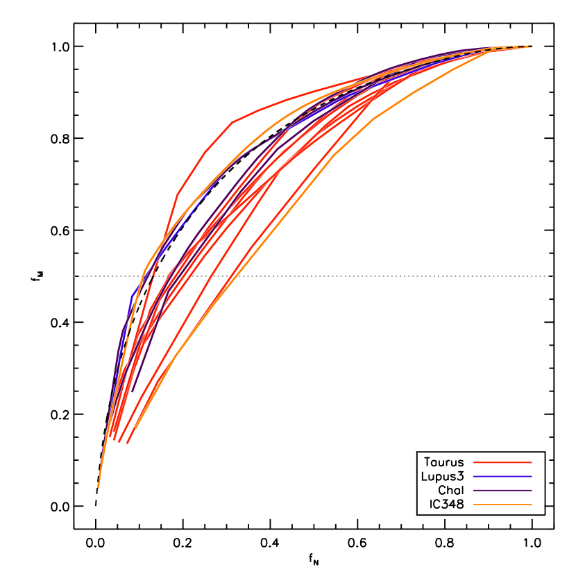
Figure 7: The fraction, $f_{M}$, of the group mass in stars having mass greater than $M$ as a function of the fraction, $f_{N}$, of the number of stars having mass greater than $M$, as $M$ decreases from the largest to smallest value for the group. The coloured curves show the values for each observed group, while the dashed black line shows the values expected for the IMF. The grey dotted line indicates a fraction of 50%.

Within each group, a significant fraction of the mass in concentrated in the few most massive members. This is illustrated in Figure 7 which shows the fraction of cumulative mass, $f_{M}$, as a function of the fraction of cumulative number of group members, $f_{N}$. While there is variation between the groups, some due to mass estimation uncertainties and some due to small number statistics, the overall trend is clear – half of the mass of the group is found within the 10-30% most massive members. This property is similar to what would be expected for cluster whose members follow the IMF. The black dashed line in Figure 7 shows the profile expected for the Kroupa IMF, using the formulation given in Weidner et al (2010), within the mass range spanned by our groups. For comparison, we also calculated the relationship expected for a symmetic, log-normal mass function, given, e.g., by Chabrier (2005), and found a nearly identical relationship to the one shown for the IMF. Both describe the relationship seen in the observed groups reasonably well. It is notable that this property of a significant portion of the group mass being found in a relatively small fraction of the group members arises for groups whose most massive members have masses much greater than the typical mass for the group, but much less than that of O stars which dominate the largest clusters.

Within clusters, the total cluster mass is correlated with either the mass of the most massive member or the total number of members (Weidner et al, 2010). While the mass of the most massive member of each group, and to a lesser extent, the total mass in the group in our dataset, are uncertain, both should be good to $\sim$50% or better. We compare the mass of the most massive member within each of our groups to the total group mass in Figure 8. In that figure, all of our groups are plotted (note that in Taurus, several of the groups have nearly identical values), along with the data in Weidner et al (2010), using the new dynamical masses for the most massive members where available. Weidner et al (2010) also derived an analytic expression for the most massive cluster member expected, based on a random sampling of the IMF, and setting the maximum mass possible for a star to be 150 M_⊙; the dotted line in Figure 8 shows the approximate linear slope found by Weidner et al (2010), assuming a Salpeter slope for the high mass tail of the IMF. Regardless of the model fit to the relationship between the most massive star and total cluster masses, it is clear that our groups follow the same trend as the clusters do.

On the other hand, the correlation between the maximum stellar mass and the total stellar mass for the groups studied here does not imply that these groups have a particular upper limit on the stellar mass for their model. The groups do not extend to high enough masses to show a reduction in slope, unlike the largest of the Weidner et al (2010) clusters shown in Figure 8 which suggested the 150 M_⊙ maximum stellar mass. At total cluster masses below 100 M_⊙, Weidner et al (2010) found their data to be consistent with a random sampling of the (Salpeter) IMF without the requirement of a maximum stellar mass.

The foregoing properties of the mass distributions in nearby groups suggest that similar physical processes are responsible for the mass distributions of stars in groups and in clusters, independent of their number of members.

4.2 Location of the Most Massive Group Member

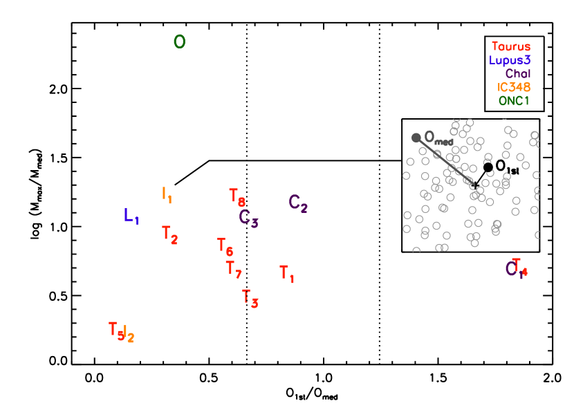
Figure 9: Mass segregation observed in the groups. The vertical axis shows the ratio in the mass of the most massive group member to the median group mass (an indication of how easily the most massive member is distinguishable), while the horizontal axis shows the ratio in offsets from the cluster centre for the most massive member and the median value. Coloured letters denote the various regions; the Trapezium cluster in Orion is also plotted for comparison. The vertical dotted lines indicate the 25th and 75th percentile values expected for a uniform random sampling of group positions. The inset shows the central part of the main IC348 group: the circles mark the positions of group members, while the plus indicates the group centre. The offset of the most massive group member, $O_{1st}$, is shown in black, while the offset of the group member at the median separation, $O_{med}$ is shown in dark grey. As shown in the main figure, $O_{1st}/O_{med}=0.3$ in this group.

Within each group, the most massive group member tends to lie close to the group centre. We find that for the fourteen groups, the median offset (or separation from the group centre) of the most massive group member, $O_{1st}$, is 0.6 times the median offset for all of the members of the same group, $O_{med}$. Figure 9 shows the ratio of $O_{1st}$ to $O_{med}$ for all of the groups. (Note that in the few groups where there were two equal mass most massive members, the one closer to the centre is used for the $O_{1st}$ calculation and the other is used for $O_{2nd}$ discussed below.) The vertical axis of Figure 9 shows the ratio of the mass of the most massive member, $M_{1st}$, and the median group member mass, $M_{med}$, indicating that in most groups, regardless of the value of $M_{1st}/M_{med}$, the most massive member of each group tends to lie nearer to the group centre than typical. For comparison, the ONC1 cluster is also shown (see Section 2.2). These results are not sensitive to the method used to determine the group centre – we find $O_{1st}/O_{med}$ values which are nearly always less than one using the centre of mass as the group centre instead of the median position.

As might be naively expected, a random distribution of group members tends to yield a ratio of offsets above and below one with roughly equal probability. We determine the ratio of offsets expected from a random uniform distribution by running 200,000 simulations for a variety of numbers of YSOs placed within a 2D circular or 3D spherical region. We measured the same ratio, $O_{1st}/O_{med}$, as described above. The vertical dotted lines on Figure 9 show the 25th and 75th percentile value of the ratio found in the random simulations for a uniform distribution of twenty five randomly distributed YSOs within a 3D sphere. These values do not change substantially for either a 2D circular distribution or a different number of YSOs in the sample. We also ran similar tests on positions following a random 3D isothermal (probability $\propto 1/r^{2}$) profile and found similar results. The 3D isothermal distribution of $O_{1st}/O_{med}$ values tends to be more peaked than the uniform distribution below $O_{1st}/O_{med}=1$, and is shallower with a long tail for values above 1 (the tail actually extends beyond $O_{1st}/O_{med}$ = 100, much larger than the range shown in Figure 9). The 25th and 50th percentile values for $O_{1st}/O_{med}$ are nearly identical for both the isothermal and uniform distributions, while the 75th percentile value tends to be larger for the isothermal than the uniform distribution. The 75th percentile value varies with the level of truncatation the isothermal distribution ($O_{1st}/O_{med}$ is $\sim 1.9$ in the absence of truncation and decreases with the degree of truncation). Regardless of the distribution adopted, the observed groups have a more centrally located most massive member than would be expected from a random distribution of positions.

As a further test of whether these massive members are more centrally located than would be expected in a random distribution, we ran simulations where we kept the group members’ positions the same, but randomized which mass belonged to each member. We did this for 10,000 trials for each group, and calculated the fraction of simulations where the most massive member had an offset ratio less than or equal to that which was observed. Where the mass segregation appears to extend to the second (and third) group member(s) (as discussed in the following subsection), we also computed the joint likelihood of having the two (or three) members with offset ratios smaller than or equal to those observed. Barring L1551 and ChaI-Southwest, whose most massive members have large offset ratios, the probabilities found for the observed group mass configurations were small – at most, around a percent, and often lower. We also ran the same test on the three least massive group members and nearly always found substantially higher probabilities, since the least massive members do not show a central concentration.

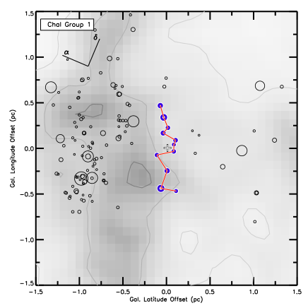
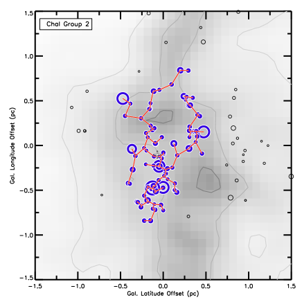
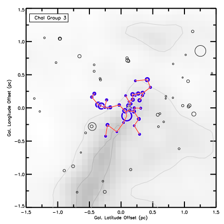
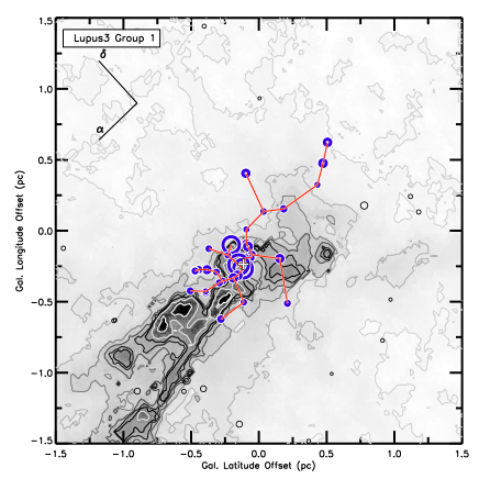
Figure 4: Groups identified in ChaI (first three panels) and Lupus3 (final panel). Directions of increasing RA and dec are shown for the first group in each region. See Figure 2 caption for more details. For clarity, the greyscale in the Lupus3 panel extends a factor of two higher in extinction than the other panels. Additional contours at 15 and 25 magnitudes are overlaid in light grey and white.

Regarding the two outlying groups, L1551 and ChaI-Southwest, it is clear that neither has the appearance of typical groups. ChaI-Southwest has a linear morphology and does not contain any particularly massive stars (Figure 4), while L1551 (Figure 3) consists of a more typically-shaped group (bottom right in figure), connected to the most massive group members (top left in figure) through a series of relatively widely spaced YSOs. Had the critical MST branch length been 5% smaller in L1551, the most massive group members would not have been considered group members, and the remaining group would show a much stronger central concentration of the most massive members. In most of the groups, the longest MST branches only connect a few low mass YSOs to the rest of the group, and the overall group structure is little affected with their inclusion or exclusion, as discussed in more detail in Appendix D.1.

While neither L1551 or ChaI-Southwest have the appearance of traditional groups, this characteristic is insufficient to explain the different behaviour between these two groups and the others. As can be seen in Figures 2 through 5, several other groups have a linear geometry (e.g., B213 / Taurus group 3) and loose spacings between members (e.g., L1527 / Taurus group 7; see also Table 1 for a comparison of median YSO spacings in each group) while still possessing a centrally-located most massive member.

4.3 Mass Segregation

The central location of the most massive group member is suggestive of a more general property of mass segregation, where more massive members are progressively more centrally concentrated. Within larger clusters, mass segregation is often observed to varying extents. For example, Stolte et al (2006) found evidence of mass segregation at all masses in NGC 3603, with the degree of segregation lessening in the lower mass bins, while Carpenter et al (1997) found mass segregation only for the most massive members of the Monoceros R2 cluster. How do the groups which we analyze compare?

In clusters, mass segregation is measured in a variety of ways including the change in slope in the mass function (or luminosity function) with radius, the ratio of the number of high- and low- mass stars as a function of radius, and the mean radius of different masses of stars (see e.g., Bonnell & Davies, 1998; Ascenso et al, 2009, and references therein). There are too few YSOs in each of the groups we identify to be able to use any of the usual mass segregation measures. We can, however, extend the offset ratio measurement discussed in the previous section to look at the distribution of offsets from the group centre as a function of mass rank.

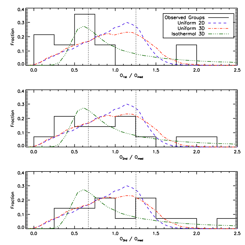
Figure 10: The distribution of offset ratios for the most massive member (top panel), second most massive (middle panel), and third most massive (bottom panel) member of each group. The blue dashed line shows the values expected for group members randomly distributed uniformly over a 2D circular area for 25 group members, while the red dash-dotted line shows the same for 25 group members randomly distributed uniformly over a 3D spherical volume, and the green dash-triple-dotted line shows the same for 25 group members in a random isothermal distribution over a 3D spherical volume. The vertical dotted lines show the 25th and 75th percentile values for the 2D uniform distribution, as shown in Figure 9.

Figure 10 shows the distribution of offset ratios for each of the three most massive members in the groups (top to bottom panels). The overplotted dashed, dash-dotted, and dash-triple-dotted lines show the distributions expected from our random simulations discussed in the previous section. The most massive group member (top panel) shows a large excess of sources with offset ratios smaller than expected from random sampling, but this excess is diminished considerably for the second most massive member (middle panel), and is gone completely for the third most massive member (bottom panel).

A simple comparison between the distribution of observed offset ratios and those found in our random 3D simulations with a two-sided KS test give probabilities of being drawn from the same parent sample of less that 0.2% for the most massive group member, and 62% and 50% for the second and third most massive members respectively for the uniform distribution, and probabilities of 0.1%, 47%, and 56% for the non-truncated isothermal distribution, with typically smaller probabilities for truncated isothermal distributions. Our largest source of error in the offset ratios is due to the definition of the centre of the groups. Using instead the centre of mass of each group to compute the offset ratios, we again find similar distributions. The two-sided KS test probabilities for the 3D uniform distribution are 0.2%, 22% and 70% for the first, second, and third most massive members respectively, and 0.2%, 10%, and 8% for the 3D isothermal distribution. The large change in the probabilities for the isothermal distribution is caused by a smaller minimum value of $O_{xth}/O_{med}$ for the observed groups using the centre of mass (instead of the median position). $O_{xth}/O_{med}$ decreases sharply for the 3D isothermal distribution below 0.5, so the KS test is highly sensitive to how low the observed $O_{xth}/O_{med}$ values extend.

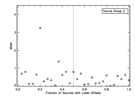
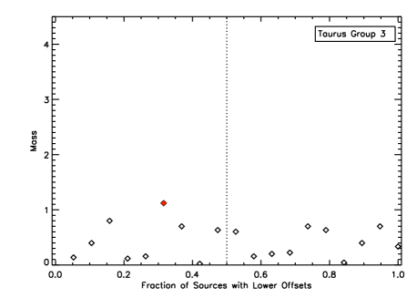
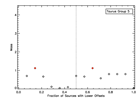
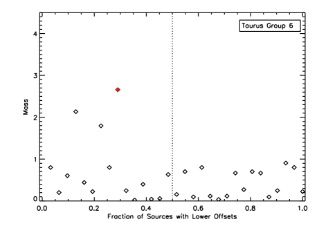
Figure 17: (This figure for the online version only) The mass of each YSO in the group versus the fraction of group members which have separations equal to or smaller than the offset of that group member. The solid red diamonds show the most massive member(s) of each group, and the vertical dotted line indiates a fraction of 50% for each group. Groups with mass segregation should have their most massive members at low fractions. Groups with complete mass segregation would follow a trend from the top left to the bottom right of the plot. Instead, we find YSOs at lower masses to be roughly evenly distributed across low and high fractions, which indicates that they are not segregated. The first six groups in Taurus are shown in this figure.

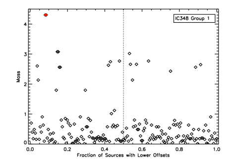
Figure 19: A continuation of Figure 17 showing the two groups in IC348. For comparison, the Trapezium cluster in Orion is also shown (bottom panel).

Figures 17 through 19 (available only online) illustrate the trend towards less-central locations with lower mass in an alternate manner, showing the mass of each source versus the order of the offsets in the group, visually confirming the statistic measures discussed above. It is interesting to note that the central location of the most massive member(s) in each group is not a function of the mass of the most massive member. In the ONC1 cluster, Hillenbrand & Hartmann (1998) found evidence for mass segregation extending down to 5 M_⊙, and possibly beyond. Visually, a similar divide is seen in Figure 19 for ONC1. Quantitatively, the offset ratio $O_{1st}/O_{med}$ is less than 1.1 for all members with masses above 4.8 M_⊙; below this mass, the maximum of $O_{1st}/O_{med}$ rapidly increases.

4.4 Massive YSOs and Clustering

Another property which our groups share with larger clusters is a central concentration. Large clusters tend to have much smaller separations between members towards the centre, coincident with where the most massive members tend to be located. While Figures 2 through 5 suggest that the most massive group members lie in or near zones with higher than average degrees of clustering within the groups, we can quantify this.

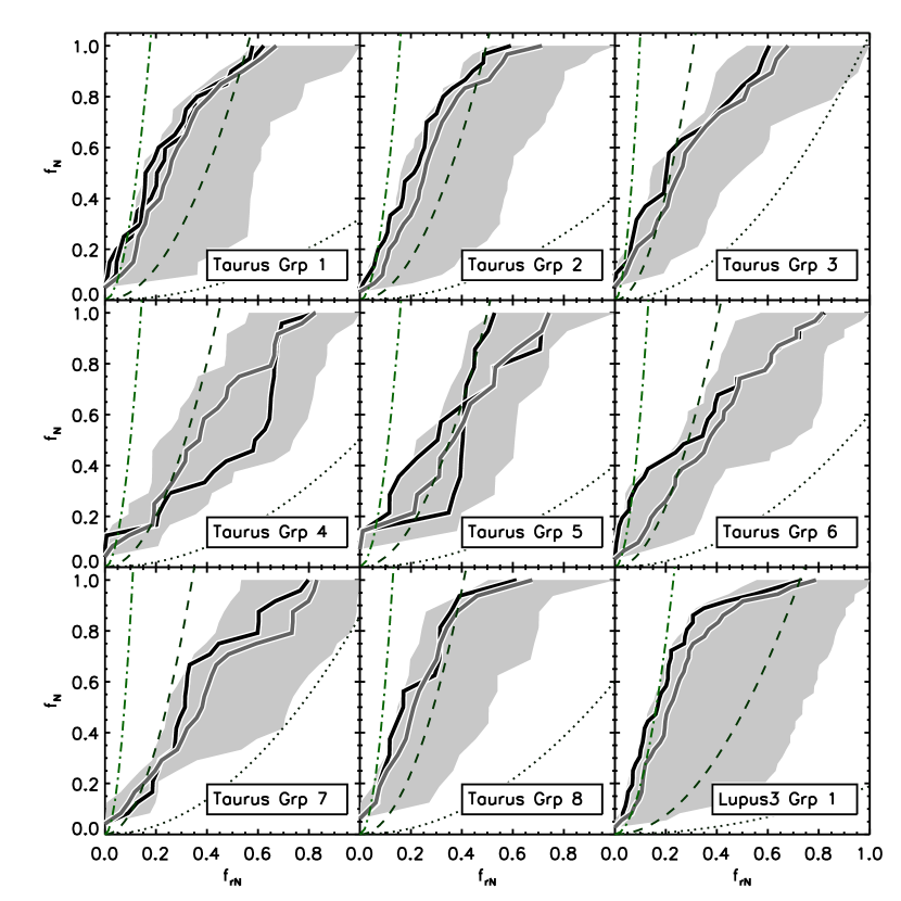
Figure 11: The fraction of the total number of group members, $f_{N}$ versus $f_{rN}$, the radius enclosing the N nearest sources from each group member normalized by the maximum value of the enclosing radius in the group. The shaded grey region indicates the range of values spanned by all group members. The black line shows the value for the most massive group member, while the grey line shows the median value for all group members. Group members located in a more clustered environment will show a steeper rise in number at low separations compared to members located in more isolated parts of the group. Lines of constant surface density are shown in green, with values of (from dark to light): 1 (dotted), 10 (dashed), and 100 (dash-dotted) pc^-2. The groups in Taurus and Lupus3 are shown in this figure; the remaining groups are shown in the following figure.

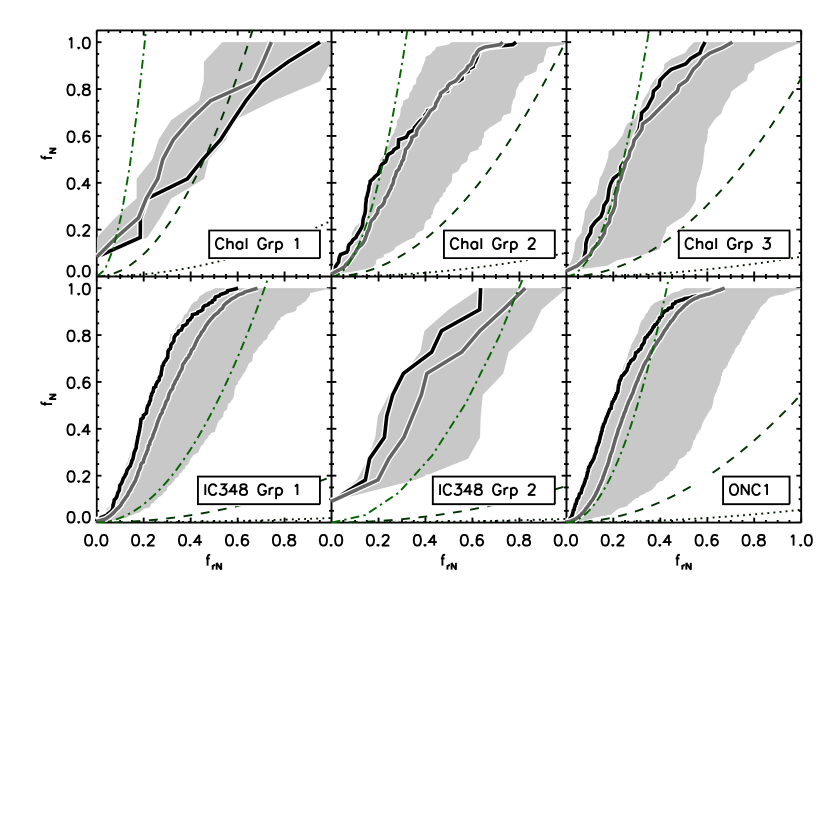
Figure 12: The fraction of the total number of group members, $f_{N}$ versus $f_{rN}$, the radius enclosing the N nearest sources from each group member normalized by the maximum value of the enclosing radius in the group for groups in ChaI (top row), IC348 (bottom row, left and middle), and the ONC1 cluster (bottom right) for comparison. See Figure 11 for the plotting conventions used.

The measurement of the surface density of stars often provides a useful criterion for determining the clustering properties. Since our groups often have a very small number of sources, these measures are more vulnerable to errors from small number statistics, and so we follow a different approach; surface density measures are discussed briefly in Section 5.1. Here, we instead compute the radius, $r_{N}$, which encloses the N nearest sources for each group member. Group members which are located near the most clustered part of the group should show a sharper rise in a plot of $N$ versus $r_{N}$ than members located in a sparser part of the group. Figures 11 and 12 show the fraction of total group members, $f_{N}$ versus $f_{rN}$, the radius $r_{N}$ normalized to its maximum value in the group for all members of each group. For clarity, all group member profiles are not shown in the figures. Instead, the range in values spanned by all members is indicated by the light grey shading, while the median profile is overlaid as the dark grey line. The most massive group member is shown in black. These plots allow comparison of the local surface density for a given radius $r_{N}$, or for a given number of neighbours N, as a function of member mass.

Figures 11 and 12 show that the most massive star is projected on a region of relatively high local surface density for a large fraction of the groups considered. The black line lies to the left of the grey line for the nine groups Taurus 1, 2, 3, and 6, Lupus3 1, ChaI 2 and 3, and IC348 1 and 2, and also for ONC1, the prototype of a large cluster with mass segregation. In contrast, the black line lies to the right of the grey line for two groups, Taurus 4 and ChaI 1. In the three groups Taurus 5, 7, and 8, the lines are too close to make a clear discrimination.

In combination with the result from Section 4.2, this result indicates that the most massive star in a group generally has a position which is central, and which is associated with a high surface density of lower-mass stars.

The tendency for the most massive member of each group to lie in a region of higher than average group member surface density can be quantified further. As already discussed, the most massive group member tends to have a profile which lies to the left of the median profile in the preceeding two figures. Put another way, for a fixed value of $f_{N}$, either $f_{rN}$ or $r_{N}$ are smaller for the most massive member than the median value. For each group, we compare $r_{N}$ for the most massive member and the median value at fixed levels of $f_{N}$. Figure 13 shows $r_{N}$ for the most massive member divided by the median value for $f_{N}=30\%$ (left panel) and 40% (right panel) for each of the fourteen groups (solid diamonds). For each group, the full range in range $r_{N}$ normalized by the median value at $f_{N}$ is indicated by the vertical line. Each vertical strip in Figure 13 therefore summarizes a horizontal cut along $f_{N}=30\%$ (left) and 40% (right) in Figures 11 and 12, normalized to the median $r_{N}$ at that $f_{N}$ (i.e., the dark grey line would always lie at 1 in Figure 13).

Plotted in this manner, it is easy to additionally compare the behaviour of the most massive member of each group with the next two most massive members, shown in Figure 13 by the open diamonds. There is some scatter between the two panels, which is expected since the most massive member and median profiles shown in Figures 11 and 12 do not remain a fixed distance apart. The two panels shown in Figure 13 are, however, representative of the general trend – we made similar figures for values of $f_{N}$ ranging from 25 to 50% in intervals of 5% and found similar results to the cases shown. Despite the scatter, it is easy to see from the plot that most of the most massive members (filled diamonds) lie near or below a value of 1 in most cases, i.e., they lie in locations which tend to be more clustered than typical for the group. The second and third most massive members only shown in Figure 13 follow this trend in only a limited number of groups.

5 DISCUSSION

5.1 Number and Surface Density

The groups that we analyze tend to have properties scaled-down, but similar to those in larger clusters. In the literature, clusters are often defined and described using criteria based on the surface or volume density of sources. Lada & Lada (2003) defined clusters as having a minimum stellar density of 1 M_⊙ pc^-3 and greater than 35 members, in order to be resistant to quick dissolution. Jørgensen et al. (2008) found that protostars in the nearby Perseus and Ophiuchus molecular clouds tended to have denser clustered substructures and used a threshold of 1 M_⊙ pc^-3 to define loose associations and 25 M_⊙ pc^-3 to define tight associations within these. A minimum number of 35 members was again used to define a cluster; associations with smaller numbers were termed groups. Porras et al (2003) similarly used a maximum of 30 members to define groups, with 31 to 100 members corresponding to small clusters and over 100 members corresponding to large clusters. Adams & Myers (2001) examined the transition between groups and clusters in more detail, and argued that groups containing roughly ten to one hundred members evolve differently than large clusters – the groups tend to disperse quickly and are likely to be unaffected by supernovae or strong UV radiation (note the number of members is higher than in Lada & Lada, 2003, as the role of gas in the cluster dissipation was also considered).

How do our groups compare? In terms of numbers of members, all but the main group in IC348 (with 186 members) fall easily within the Adams & Myers (2001) definition of a group, and many also do so with the N=30-35 definition of Lada & Lada (2003), Jørgensen et al. (2008), and Porras et al (2003). In terms of surface density, our groups tend to also lie below the standard cluster values.

Figures 11 and 12 show lines of constant surface density from 1 to 100 pc^-2 separated by factors of ten. In the Taurus and Lupus3 groups, values tend to range from a minimum of around 1 pc^-2 to a few times 10 pc^-2. The ChaI groups tend to have slightly larger surface densities (particularly ChaI-Southwest / Group 1), while the IC348 groups have surface densities nearly 100 times larger. The embedded clusters in the sample of Gutermuth et al (2009) tend to have much higher surface densities, typically peaking around a few hundred per square parsec. Assuming, as in Jørgensen et al. (2008), spherical symmetry and a typical YSO mass of 0.5 M_⊙, then the volume density thresholds of 1 and 25 M_⊙ pc^-3 correspond to roughly twice those values in number per square parsec for surface density. The groups in this paper are denser than their surroundings, but are generally much less dense than those considered in any of the above-cited works.

5.2 Predictions of Mass Segregation

In most of the groups, we find the single (or, for L1356, Lupus3-main, and IC348-main, several) most massive group member(s) are located near the group centre, and near a region of higher than average surface density of sources. Mass segregation is often observed in large clusters, with some regions showing evidence of segregation at all masses, with the degree of segregation lessening in the lower mass bins (e.g. Stolte et al, 2006), while other regions appear to show mass segregation only for the most massive members (e.g., Carpenter et al, 1997). One complication in mass segregation measurements in clusters, particularly more distant clusters, is the observational bias due to crowding. Ascenso et al (2009) argue that this bias, which leads to increasing levels of incompleteness in the lower mass objects at smaller cluster radii, may be partially or even fully responsible for the observed mass segregation in clusters. The central location of the most massive cluster members would appear to be robust, however, since these stars would be easily detectable in the outskirts of the clusters as well.

The young age of some of these clusters, coupled with the degree to which the most massive cluster members are concentrated in the centre has led to the argument that at least some of the observed mass segregation is primordial, rather than dynamical (e.g. Bonnell & Davies, 1998). More recently, Moeckel & Bonnell (2009) have argued that the primordial mass segregation must be confined to only the most massive stars, as any initial amount of mass segregation in the lower-mass population leads to an over-prediction of the mass segregation that should be currently observable in those clusters. Other work has questioned whether any primordial mass segregation is required (Allison et al, 2009) to match present-day observations of clusters.

In the groups we study, the mass segregation observed for the most massive members appears to require an early central concentration of these objects. The groups have ages around 1 Myr, while the crossing times are typically between 1-3 Myr, assuming a velocity dispersion of 1 km s^-1 (the approximate value found in the proper motion groups in Taurus in Luhman et al, 2009). Since there are too few group members for the scenario simulated in Allison et al (2009) to be applicable, it seems that the most massive members of the groups must have formed near the group centres, rather than migrating there later. For the majority of their lifetime, the YSOs have been embedded in their natal gas, hence the timescale for dynamical evolution can be estimated as

$$t_{relax}=\frac{N\epsilon^{-2}}{10ln(N/\epsilon)}t_{cross}$$ (1)

where $N$ is the number of stars, $\epsilon$ is the star formation efficiency of the group, and $t_{cross}$ is the crossing time of the group (Adams & Myers, 2001). For a star formation efficiency value of 10%, the relaxation timescale is nearly five times the crossing time for the smallest groups, and becomes larger for both larger groups and lower star formation efficienies; the relaxation timescale well exceeds 5 Myr for the groups under any reasonable assumption of the star formation efficiency. Given the ages estimated for the groups, the central locations of the most massive members cannot be wholly attributed to dynamical relaxation.

Some degree of early mass segregation appears to be consistent with models for massive star formation. In the competitive accretion scenario, protostars forming in the centre of the cluster potential inhabit a higher density environment and hence accrete more mass than those formed at the cluster periphery (e.g., Bonnell et al, 2001). In the monolithic collapse scenario (McKee & Tan, 2003), stars form out of quasi-equilibrium clumps. Clusters require several times the dynamical timescale to form, which enables mass segregation to occur in a greater amount than would be anticipated from a faster formation scenario (Tan et al, 2006). In the stationary accretion model of Myers (2009b), high mass stars are only able form in the densest environments, where the accretion rate is highest, while lower mass stars are able to form in the surrounding higher and lower density environments. It is unclear, however, whether these models can predict the clear transition between the location of the most massive few group members and the other group members, or, in some cases, operate at all for such small groups.

Association of the most massive star with a high surface density of lower-mass stars tends to rule out a very simple cluster formation scenario, where the massive star accretes all the mass within a certain radius, causing a local minimum in the density of lower-mass stars. Instead, it may be more realistic that a spherical zone around an accreting massive star feeds the massive star as well as numerous lower-mass stars (Smith et al, 2009; Wang et al, 2010).

In their Herbig Ae/Be survey, Testi et al (1999) found instances where the massive star appeared to be relatively isolated, as did Massi, Lorenzetti & Giannini (2003) in their survey of luminous IRAS sources in the Vela C and D molecular clouds. We also find a few instances of isolated massive stars in our catalogs – one A2 star in Taurus, one B6.5 and one F0 star in ChaI, one B4 star in Lupus3, and several A stars in IC348 which fall near but outside of the main group. These sources represent a much smaller fraction of isolated early-type sources than were found in Testi et al (1999)’s work, suggesting that isolated A and B stars are uncommon in young star-forming regions. Future observations may lower this fraction even further, either with evidence that these apparently isolated stars are interlopers or the discovery of more lower mass members nearby. The isolated early-type star in Lupus3, for example, lies well outside the main group, where there have likely been fewer surveys for low mass members in the region.

6 CONCLUSION

We present a study of groups of young stars within four nearby star-forming regions – Taurus, Lupus3, ChaI, and IC348. The census of stars within each of these regions is complete down to very low masses, typically late-M, corresponding to $\sim$0.02 M_⊙. YSO masses are estimated from spectral types following Luhman et al (2003). Using a minimal spanning tree algorithm and following the procedure of Gutermuth et al (2009), we identify fourteen groups of YSOs within the regions, with the total number of members ranging from 11 to 186, with most in the range of 20 to 40. The total number and surface density of group members tends to be smaller than in clusters by a factor of five to ten, or more. The groups are sufficiently young that their configurations should be similar to their primordial configuration.

Within these groups, we find the following:

1. The groups have a wide range in masses; the maximum mass member is typically more than five times the median member mass.

2. The maximum member mass and total group mass are correlated and follow a similar relationship to that seen in clusters.

3. Most of the mass in each group is found in a small fraction of the group members.

4. In most groups, the most massive star tends to be centrally located. In a few groups, this property extends to the second- or third- most massive star.

5. In most groups, the most massive star is associated with a relatively high surface density of lower-mass stars.

6. The central concentration of massive stars is much more than expected for a random distribution YSOs.

7. The central concentration of massive stars occurs even if the most massive star is only 1 M_⊙.

Due to the proximity and sensitivity of the coverage of these star-forming regions, our analysis does not suffer from the problems of crowding and variable completeness which may affect more distant clusters (e.g., Ascenso et al, 2009). The similarity in the properties of these small groupings of stars therefore offers a complementary avenue to explore the some of the processes which influence massive cluster-forming regions which are more distant.

Appendix A ADOPTED SOURCE CATALOGS

A.1 Taurus

We analyze the 352 Taurus members discussed in Luhman et al (2009) and given in Table 7 of Luhman et al (2010, hereafter L10). For the binary pair HD 28867A+C and B, we adopt the positions given in Walter et al (2003); the L10 catalog names correspond to identical positions for both sources. Where the data exists, members were confirmed using proper motion data, as discussed in the appendix of Luhman et al (2009). Otherwise, membership was based on a variety of observations including Ca II emission, H $\alpha$ emission, X-ray data, spectral energy distributions, and / or spectra from optical through far-IR observations (e.g., Kenyon et al, 2008). Table 3 (available online) summarizes the data – the position, L10 name(s), spectral type, estimated mass (Section 2.1 and Appendix C), and the group (Section 3). Some of the spectral types are highly uncertain, and were estimated based on the bolometric luminosity of the source, as indicated by footnotes in Table 3. In these cases, the spectral type and mass should be treated as being in the range given in the footnote.

The Spitzer Taurus team has also published a full catalog of YSOs in Taurus, including both Spitzer photometry of previously known members and new and candidate members based on Spitzer photometry, and in many cases, additional follow-up spectroscopy (Rebull et al, 2010, hereafter R10). For the analysis discussed in this paper, we use the L10 catalog because it spans a larger area of the cloud – the R10 catalog covers only the region mapped by Spitzer. Our results are largely unchanged when using the R10 catalog instead, as described in more detail in Appendix B.

We adopt a distance of 140 pc to the Taurus cloud, following Torres et al (2007).

A.2 ChaI

In ChaI, we analyze 237 sources whose properties are summarized in Table 4 (available online; the same columns are used as in Table 3). This list includes the 226 known members of ChaI discussed in Luhman (2007); 215 of these sources are given in Table 6 of Luhman (2007), while the remaining 11 were excluded because they lacked accurate spectral types. These 11 sources are J11094192-7634584 and J11095505-7632409 from Table 5 of Luhman (2007), J11011926-7732383B from Table 1 of Luhman (2004b), and Ced110-IRS4, ISO86, Ced110-IRS6, ISO97, B35, IRN, ISO192, and ISO209 from Table 5 of Luhman (2004a). We also add the 8 new members identified in Table 1 of Luhman & Muench (2008) and 4 new members identified in Table 4 of Luhman et al (2008). Following the discussion in Luhman et al (2008), ISO130 was excluded, as it is likely a galaxy, and sources J11183572-7935548, J11334926-7618399, J11404967-7459394, and J11432669-7804454 were removed as their proper motions indicate they are more likely to be members of $\eta$ Cha than ChaI. Additionally, four new members were added : RXJ1129.2-7546, RXJ1108.8-7519a, RXJ1108.8-7519b, and Cha-MMS1, for which proper motion measurements indicate that they are likely ChaI members. As with the Taurus catalog, proper motion data was used where available to verify membership, otherwise, a variety of indicators of youth were used.

Following the discussion in Luhman (2008b), we adopt a distance of 160 pc to the region.

A.3 Lupus3

In Lupus3, we analyze 70 YSOs (Table 5, available online) from the compilation of Comerón (2008). We include all of the sources in Comerón’s Table 11 (well-known classical T-Tauri stars from Thé, 1962; Krautter et al, 1997; Hughes et al, 1994), Table 14 (additional low-mass members from Comerón et al, 2003) and Table 16 (possible low mass members of Lupus3 from López Martí et al, 2005). The source list in Table 16 in Comerón (2008) gives less accurate positions than in López Martí et al (2005), so we use the original data.

We do not include the sources given in Comerón’s Table 13 (suspected Lupus3 members from Nakajima et al, 2000), as the survey these data originate from only spans an RA of roughly 16:09:44 to 16:08:44 (in J2000), which is much smaller than the region spanned by the Lupus3 group. Inclusion of these sources could bias the clustering statistics due to their limited areal range (which is not centred on the apparent group centre), and furthermore the spectral types of all of these sources are unknown. We also exclude the list of weak T-Tauri stars in Lupus3, as these stars are thought to be older and not associated with the current groups (Comerón, 2008).

We adopt a distance to Lupus3 of 200 pc, as recommended by Comerón (2008).

A.4 IC348

In IC348, we analyze a total of 363 sources whose properties are given in Table 6 (available online). This includes the 307 sources listed in Lada et al (2006, Table 2) and the 41 sources identified in Muench et al (2007, Table 1). We supplement this list with all other likely members with known spectral types: seredipitously discovered members 273 and 401 discussed in Appendix C of Muench et al (2007), as well as source 30074, the companion of 166 (Luhman et al, 2005, and listed as 166B there), and 8078, the companion of 9078 (Luhman et al, 2003, listed as 78B and 78A respectively there). We use updated spectral classifications for 7 of the sources in the Lada et al (2006) catalog (141, 174, 294, 334, 366, 1050, and 2103), and also add 11 sources with spectra (249, 250, 307, 313, 340, 1686, 1779, 1840, 6005, 10074, and 10095) recently obtained by K. Luhman (private communication). Note that in the Muench et al (2007) catalog, where there are multiple spectral classifications, we use the optical classification.

We adopt a distance of 300 pc, following the discussion in Herbst (2008).

A.5 Completeness

The YSO catalogs of all four regions have good completeness. In Taurus, a comparison of X-ray and optical/IR survey data shows the catalog should be complete to $\sim$0.02 M_⊙ for class II and III stars and brown dwarfs. The completeness is good for class I stars, but is difficult to determine for class I brown dwarfs (later than $\sim$M6) due to confusion in Spitzer bands with faint red galaxies (Luhman et al, 2009). Well-known young protostars such as L1527-IRS1, L1521F, and IRAM 04191+1522 are included in the catalog. Other candidate class 0/I protostars with very weak Spitzer fluxes may be missing, such as J041757.75+274105.5 (Barrado et al, 2009). Using the overly conservative estimate that all class I brown dwarfs and class 0 sources are missing from the catalog suggests only 6% of the total number of sources are missing from the catalog, using the ratio of classes of objects given in Evans et al (2009).

López Martí et al (2005) estimate they are complete in Lupus3 down to an R-band magnitude of 20 and and I-band magnidue of 19, which corresponds to $\sim$0.02 M_⊙ at 1 Myr and 0.03 M_⊙ at 5 Myr in the Chabrier et al (2000) models, at a distance of 200 pc. The completeness level is not explicitly given in the Hughes et al (1994) sample of T-Tauri stars. In the brown dwarf mass regime, the Lupus3 sample may be less complete than in Taurus; Comerón (2008) lists several additional studies with lists of candidate members that have not yet been spectroscopically-confirmed. In particular, sources detected only in Spitzer have not yet had spectroscopic follow-up, so it is likely that most, if not all, class I sources are not included in our analysis. Class I sources consistute only $\sim 4-5\%$ of the population in Lupus3 (Merín et al, 2008), however.

The ChaI catalog described in Luhman (2007) was found to be complete for masses above 0.01 M_⊙ in regions where A${}_{J}\leq 1.4$ mag. Spitzer data was not used for that catalog, hence class I sources are likely missing. Subsequent spectral surveys (Luhman et al, 2008; Luhman & Muench, 2008) based on Spitzer data do include a limited number of class I sources (four or five). If the class I population in ChaI is similar to that in ChaII (Evans et al, 2009), then roughly one quarter of the class I’s are currently included in the catalog, implying only $\sim$7.5% of the total sources are missing from the catalog.

In IC348, the central region covered in the Luhman et al (2003) catalog was found to be complete to $\sim$0.03 M_⊙ for $A_{V}<4$ mag. The Spitzer data included in Muench et al (2007) identified very few new members within the Luhman et al (2003) survey bounds, and instead extended the catalog to larger distances from the centre, with an estimated completeness of $>$80% for YSOs with H-band magnitudes of 16; this corresponds to a mass of $\sim$0.015 M_⊙ at 1 Myr and 0.02 M_⊙ at 5 Myr in the Chabrier et al (2000) models, at a distance of 300 pc. In the Muench et al (2007) dataset, a total of 20 class 0/I sources were identified, corresponding to $\sim$6% of the total. Other work (Jørgensen et al., 2008) suggests that the fraction of class 0/I sources is $\sim 9\%$ of the total IC348 population, which implies that only roughly 3% of the total sources are missing from the catalog.

Appendix B ALTERNATE CATALOG OF TAURUS YSOS

Two groups have independently released Taurus YSO catalogs recently – L10 and R10. We adopted the L10 catalog in our analyses because of the wider spatial coverage. While not identical, the bulk of the catalogs agree within the area covered by R10 (i.e., the extent of the Spitzer coverage). The R10 catalog contains several types of listings – definite members (previously identified and newly confirmed members), as well as candidate YSOs described both by a likelihood of membership (probable or possible member, needing additional spectroscopic follow-up and pending spectroscopic follow-up), in addition to a rank (likelihood of membership given the available data, ranging from A+ to C-). Within a central part of the Spitzer coverage (4:15:45 to 4:35:45 in RA and 23:15:00 to 27:00:00 in dec), we found 79 sources common to both catalogs, 2 additional un-matched sources in R10 and 7 additional un-matched sources in L10, of which 6 were unresolved secondaries in the R10 catalog. Where the sources are listed in both, the agreement in spectral classification is generally quite good – 77% agree within the expected error of 1 spectral sub-class, and an additional 11% have no spectral classifications in R10. Only 5% of the sources have classifications that differ by more than two sub-classes, and some of those are listed as being uncertain classifications in each paper. [These numbers are for the definite members in R10 catalog only; the fractions are nearly identical when including the candidate members, since there are few (or no) additional matches for each broader R10 category.]

We ran all of our analysis on the R10 catalog and found similar results to those using the L10 catalog. Two of the Taurus groups we identified in L10 (L1551 and L1517) fall outside the spatial range covered by the R10 catalog. All remaining groups were recovered, although one group (L1536) was split into two groups. The critical branch length fit for the R10 stars was nearly 10% smaller than the value found in the L10 catalog, causing the linkage between the most clustered part of the group to become separated from the more filamentary part of the group. As with the L10 Taurus groups, the R10 Taurus groups nearly always had the most massive group member(s) located near the centre of the group, and in or near the region of highest surface density of sources. Our conclusions are therefore unaffected by the choice in source list for Taurus.

Appendix C MASS ESTIMATION

We adopt the conversion between spectral type and effective temperature used by Luhman (2004a) with the addition from Luhman et al (2008) of a temperature of 2200 K for L0 stars. The full set of effective temperatures we adopt is included in Table 2. We then follow the procedure of Luhman (e.g., see discussion in Appendix B of Luhman et al, 2003), using several different stellar evolution models to estimate the mass based on the effective temperature, which are outlined in more detail below. The mass we estimate for each spectral type is also given in Table 2.

Above 1 M_⊙, we use the Palla & Stahler (1999) models at an age of 1 Myr. All of their models adopt a ratio of mixing length to local pressure scale height of 1.5, and a helium fraction, Y, of 0.28.

Between 0.6 and 1 M_⊙, we use the Baraffe et al (1998) models with a mixing length of 1.9 (and Y of 0.282). The youngest ages available in these models are 2 Myr, which we adopt. Despite having twice the age of the Palla & Stahler (1999) models, there is good agreement between the two models at 1 M_⊙.

Between 0.1 and 0.6 M_⊙, we use a different set of the Baraffe et al (1998) models – those with a mixing length of 1 (and Y of 0.275), and again the youngest available age of 2 Myr. These models were run on a much finer grid than the mixing length of 1.9 Baraffe models, particularly at the lower mass regime, and hence provide a much more precise estimate of the mass based on effective temperature. The mixing length 1 models are not in agreement with the Palla & Stahler (1999) models at 1 M_⊙, hence cannot be used for the entire range. At 0.6 M_⊙, they are consistent with the mixing length 1.9 Baraffe et al (1998) models, and hence this is a reasonable mass at which to switch the model used.

Below 0.1 M_⊙, the Chabrier et al (2000) models at 1 Myr are used. This has good agreement with the Baraffe et al (1998) models with mixing length of 1 at 0.1 M_⊙. None of the other models extend to such low masses, and so cannot be used in this regime.

Figure 14 shows the mass versus the effective temperature given in the above models. The transitions between the various models are indicated by the horizontal dotted lines. The transition between models is relatively continuous, thus the combination of models is reasonable. Comparison with D’Antona & Mazzitelli (1994) model 1, over its full range in masses (0.02 and 2.5 M_⊙), and again adopting the Luhman temperature scale, we find the D’Antona & Mazzitelli (1994) models predict that the stars are $\sim$30% less massive. This is slightly smaller than the uncertainty due to assuming a single constant age, as discussed in Section 2.1.

C.0.1 A Note on Uncertainties in Spectral Types

The spectral types are typically uncertain to one subclass (K. Luhman, private communication). As can be seen in Tables 3 through 6, however, there are some instances of uncertain or unknown spectral types in most of the regions, which are discussed below.

Sources with limits on their spectral types (e.g., less than K5) are assigned a spectral type equal to the limit for the purpose of estimating the mass (this affects three, four, and two sources in Lupus3, ChaI, and IC348 respectively). Sources with a range in spectral types given are assigned to the midpoint spectral type for the mass calculation (two K7-M0 sources in Lupus3). Finally, sources with completely unknown spectral types are assigned to have the median mass of YSOs in their region, in order to avoid bias in our later analysis (five, eleven, and seven soures in Lupus3, ChaI, and IC348 respectively).

Only some of the sources with uncertain spectral types fall within the groups we analyze. In Taurus, 16 of the 31 sources with spectral types estimated from bolometric luminosities (Appendix A) are group members; none are the most massive few members, hence the uncertain spectral type has minimal impact on our analysis. All of the sources with uncertain spectral types in ChaI fall within ChaI-South (12 of 96 group members) and ChaI-North (3 of 43 group members), and again do not have mass rankings within the top few group members. In Lupus3, none of the sources with uncertain spectral types fall within the group, and in IC348, only one falls within IC348-North.

Appendix D GROUP IDENTIFICATION

D.1 MST Critical Branch Length

The definition of the groups we identified relies on the value used for the critical MST branch length; larger values tend to increase the number of group members, while smaller values tend to decrease the number of members. Figure 15 shows our method for determining the critical branch length – the cumulative distribution of MST branch lengths is well-described by a steep linear rise at small branch lengths, followed by a turn-over and a shallow linear rise at large branch lengths. Figure 15 shows the data for ChaI; the other three regions show a similar trend. Following Gutermuth et al (2009), we make linear fits to the two ends of the distribution, and define the critical branch length as the length at which the two best-fit lines intersect. For each of the four regions, we tested the range of possible critical values that could be fit, and found that the variation was less than 10% for all regions, and less than 5% in IC348.

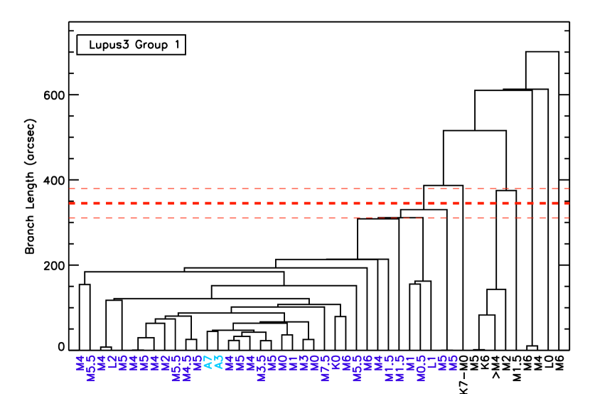
Figure 16: The dendrogram structure for the main group and nearby YSOs. The spectral type of each Lupus3 group member (blue), and the ten nearest sources beyond the group (black) are shown along the horizontal axis. The most massive members in Lupus3 are shown in pale blue. The thick horizontal dashed line indicates the critical branch length measured in Lupus3, while the thin dashed lines show $\pm 10\%$ of this value.

We examined the effect on the group definitions of a 10% larger or smaller critical branch length. One way to examine this is through a dendrogram (used recently for analyzing structure in 3D data cubes in Rosolowsky et al, 2008, for example). Figure 16 shows the dendrogram of the main group in Lupus3. The MST branch length connecting two sources is shown on the vertical axis at the connection of each pair of sources or previously connected nodes. The thick dashed horizontal line shows the critical branch length measured in Lupus3, while the two thin dashed lines indicate a range of $\pm 10\%$ around the critical branch length.

In the Lupus3 group, clearly most of the members are tightly clustered with separations well below the critical branch length. An increase in the critical branch length of 10% would increase membership by only one late-type source and a decrease of 10% would result in the group decreasing by two or up to six late-type YSOs (90% of the critical branch length is very nearly equal to the branch length required to joining four of the outlying group members to the rest of the group).

Most of the other groups show a similar behaviour – an increase or decrease of the critical branch length by 10% changes the group membership by at most a handful of members (most often one or two). In the main group in IC348, the number of group members included / excluded by a variation in the critical branch length is larger, but still a small fraction ($<5\%$) of the total number of members. The other exceptional group is L1536, also discussed in Appendix B – the critical branch length is only marginally larger than the branch length connecting two sub-groupings of YSOs, and would be split into two groups with a slightly smaller critical branch length, as occurred with our analysis using the R10 catalog. L1527 also shows a similar behaviour although to a lesser extent – two smaller sub-groups would be lost if the critical branch were reduced by 5 to 10%, but the structure as a whole is more robust to smaller perturbations in the critical branch length.

In terms of our analysis, the variation in the number of group members is less important than the impact on the relationship between the most massive group members and the rest of the group. In the Lupus3 group, as seen in Figure 16, the most massive group members lie in a much more highly clustered part of the group (as found in Section 4.4), and their relationship with the bulk of the group is little affected by the loss or gain of YSOs at the group outskirts. A similar result is found upon examination of dendrograms of most of the other groups and their nearest neighbours. As expected, the two groups whose most massive member is not centrally-located (ChaI-Southwest and L1551) are more liable to be excluded from the group structure if the critical branch length is decreased sufficiently. In L1536, if the group is split in half, each piece has a centrally-located most massive member.

D.2 Other Cluster-Identification Algorithms

The MST algorithm identifies groups by linking members together through their closest neighbour, referred to as a ‘single linkage’ technique for cluster- (or group-) identification. In fields outside of astronomy, the MST technique is often less popular than other linkage techniques which are better-suited for identifying round clusters (private communication, E. Feigelson). There are two other main classes of routines – ‘average linkage’, which use the distance of an object to the cluster centre, and ‘complete linkage’, which use the distance of an object to the furthest cluster member (Feigelson & Babu, in prep); the latter is useful for identifying very concentrated clusters.

We experimented with both techniques to identify groups in our dataset, using IDL’s cluster_tree function. As with the MST or ‘single-linkage’ technique, the maximum linkage length to define a group must still be chosen. We use the same method as we adopted for the MST, i.e., the critical length, measured using the cumulative distribution of lengths (discussed in more detail in Appendix D.1). Since the distance to a group’s centre or furthest member is larger than to the nearest neighbour, the critical lengths fit for the average and complete linkage techniques tend to be significantly larger than the value we found for the MST analysis. A (small) range of critical lengths can provide a good fit to the cumulative distribution; for reasons that will become apparent below, we use the largest critical length possible.

Using the most conservative complete linkage technique, only small groupings are identified in our dataset. IC348, for example, is split into four groups, each with only a handful of members, which do not appear as visually distinct groupings. In our MST analysis, 182 members were found in the main group of IC348. In Taurus, only three groupings are identified; other visually striking groupings identified using independent methods (Section 3.2) are missed. We therefore conclude that these young nearby stellar groups are too sparse to be effectively identified using the complete linkage technique.

Using the less conservative average linkage technique, we have mixed results. In Lupus3 and Taurus, most visually-striking groupings are identified. There is a good correspondence between these groups and the MST groups, although the average linkage groups tend to have fewer members. In Taurus, two of the eight groups identified with the MST (B213 and L1527) are no longer large enough to meet our minimum membership criterion ($>10$ members), and one MST-identified group becomes split in half (L1536, discussed in Appendix D.1 for a similar reason). In ChaI and IC348, however, we encounter a similar problem as found with the complete linkage technique – the groups identified are overly-subdivided and do not appear visually distinct. IC348, for example, is split into 8 groups, most of which border directly on several other groups and do not appear to be separate. The ChaI-south group identified using MSTs is similarly split into four groups with the average linkage technique. This fragmentation occurs despite the fact that we pushed the linkage length to the upper end of the range possible. In our datasets, it therefore appears that these other linkage techniques are overly sensitive to small-scale substructure perturbations, and are not optimal for identifying groups.

In Taurus and Lupus3, where the average linkage technique works, the most massive group members have a small offset from the centre. The $O_{1st}/O_{med}$ values found are slightly smaller than those measured with the MST groups.

Table 1: Properties of groups identified

Region	#	centre RA	centre Dec	N	Mmed	Mmax	Omed	O1st	Lcrit	Lmax	Lmed	Description
		(J2000.0)	(J2000.0)		(M⊙)	(M⊙)	(pc)	(pc)	(pc)	(pc)	(pc)
Taurus	1	4:14:25.07	28:10:13.75	20	0.426	1.796	0.282	0.228	0.520	0.516	0.127	B209
Taurus	2	4:18:51.68	28:23:46.33	30	0.398	3.250	0.400	0.118	0.520	0.448	0.135	L1495E
Taurus	3	4:21:28.19	27:02:57.18	19	0.398	1.121	0.512	0.330	0.520	0.481	0.168	B213
Taurus	4	4:32:15.48	18:17:42.35	24	0.684	3.250	0.551	1.005	0.520	0.498	0.182	L1551
Taurus	5	4:32:34.07	24:22:18.58	14	0.684	1.121	0.452	0.028	0.520	0.508	0.193	L1529
Taurus	6	4:35:17.03	22:56:09.92	31	0.398	2.659	0.685	0.367	0.520	0.511	0.221	L1536
Taurus	7	4:40:36.82	25:52:09.08	24	0.575	2.616	0.707	0.406	0.520	0.506	0.231	L1527
Taurus	8	4:55:49.24	30:30:57.12	16	0.213	3.250	0.343	0.202	0.520	0.475	0.125	L1517
Lupus3	1	16:08:29.53	-39:05:54.72	36	0.271	3.019	0.271	0.035	0.335	0.320	0.077	Lupus3-main
ChaI	1	11:02:56.17	-77:21:40.87	12	0.201	0.906	0.250	0.449	0.210	0.209	0.135	ChaI-Southwest
ChaI	2	11:08:26.16	-77:28:52.22	96	0.236	3.246	0.445	0.378	0.210	0.190	0.066	ChaI-South
ChaI	3	11:09:40.23	-76:31:20.94	43	0.303	3.250	0.212	0.134	0.210	0.188	0.066	ChaI-North
IC348	1	3:44:33.96	32:08:16.75	186	0.271	4.303	0.244	0.072	0.083	0.082	0.034	IC348-main
IC348	2	3:44:33.10	32:14:51.26	11	0.335	0.531	0.064	0.008	0.083	0.083	0.048	IC348-North

Table 2: Adopted Mass Estimates

Spectral Type	Teff (K)	Mass (M⊙)	Spectral Type	Teff (K)	Mass (M⊙)
B5	15400	4.303	G2	5860	2.632
B6	14000	3.725	G3	5830	2.627
B7	13000	3.652	G4	5800	2.621
B8	11900	3.397	G5	5770	2.616
B9	10500	3.250	G6	5700	2.602
A0	9520	3.165	G7	5630	2.587
A1	9230	3.124	G8	5520	2.562
A2	8970	3.076	G9	5410	2.535
A3	8720	3.019	K0	5250	2.430
A4	8460	2.949	K1	5080	2.265
A5	8200	2.891	K2	4900	2.134
A6	8050	2.864	K3	4730	1.796
A7	7850	2.834	K4	4590	1.634
A8	7580	2.802	K5	4350	1.121
A9	7390	2.783	K6	4205	0.906
F0	7200	2.768	K7	4060	0.801
F1	7050	2.756	M0	3850	0.701
F2	6890	2.744	M1	3705	0.633
F3	6740	2.733	M2	3560	0.575
F4	6590	2.721	M3	3415	0.398
F5	6440	2.707	M4	3270	0.271
F6	6360	2.699	M5	3125	0.178
F7	6280	2.690	M6	2990	0.096
F8	6200	2.681	M7	2880	0.057
F9	6115	2.670	M8	2710	0.031
G0	6030	2.659	M9	2400	0.013
G1	5945	2.646	L0	2200	0.009

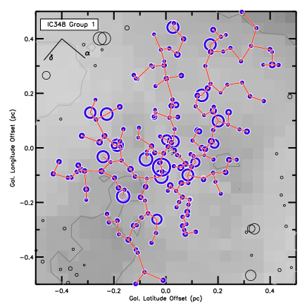
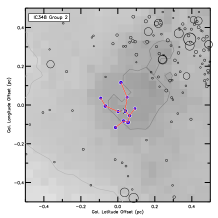
Figure 5: Groups identified in IC348. See Figure 2 caption for more details. Note the linear scale is a factor of 3 smaller in these plots than the previous ones. The direction of increasing RA and dec is shown in the first panel.

Figure 6: The distribution of masses within the main IC348 group (solid line). The dotted line shows what would be expected from the IMF, using the formulation given in Weidner et al (2010), with the minimum mass set equal to that in the observations and scaled to the total number of YSOs in the main IC348 group.

Figure 13: A comparison of the local surface density of YSOs around the most massive group member relative to typical values in its group. Each vertical line represents the data taken along a horizontal cut of Figures 11 and 12 for each group at $f_{N}=30\%$ (left panel) and 40% (right panel). Values in this figure are normalized to the median value of $r_{N}$ for each group at $f_{N}=30\%$ and 40%. The vertical lines show the range of (normalized) $r_{N}$ (light grey shading in the previous figures) for the specified values of $f_{N}$, and the solid diamond shows the (normalized) $r_{N}$ for the most massive group member (black line in the previous figures). The open diamonds show the (normalized) $r_{N}$ for the second and third most massive group members. Members with (normalized) $r_{N}$ values below 1 lie in the most clustered parts of their group.

Figure 14: The mass estimate based on effective temperature given by the stellar evolution models adopted (diamonds). The horizontal dotted lines indicate the transition between the various stellar evolution models used: Palla & Stahler (1999) above 1 M_⊙, Baraffe et al (1998) between 0.6 and 1 M_⊙ and 0.1 and 0.6 M_⊙, and Chabrier et al (2000) between 0.01 and 0.1 M_⊙. The effective temperature of selected spectral types are indicated along the top of the plot. See Appendix C for more details.

Figure 15: The determination of the critical branch length for a region. Plotted is the cumulative number of branches with length x or smaller in the ChaI region. The two ends of the distribution are well fit by straight lines. The critical branch length is defined as the intersection between these two lines. See Appendix D.1 for more details.

Appendix E Online Material

Table 3: YSO catalog for Taurus

RA	Dec	Name	Other	Spectral	Est. Mass	Group
(J2000.0)	(J2000.0)		Designation	Type	(M⊙)
4:03:49.31	26:10:52.03	J04034930+2610520	HBC358A+B+C	M3.5	0.335	–
4:03:49.98	26:20:38.23	J04034997+2620382	XEST06-006	M5.25	0.157	–
4:03:50.84	26:10:53.20	J04035084+2610531	HBC359	M2	0.575	–
4:04:39.37	21:58:18.65	J04043936+2158186	HBC360	M3.5	0.335	–
4:04:39.85	21:58:21.53	J04043984+2158215	HBC361	M3	0.398	–
4:04:43.07	26:18:56.39	J04044307+2618563	IRAS04016+2610	K3	1.796	–
4:05:30.88	21:51:10.68	J04053087+2151106	HBC362	M2	0.575	–
4:08:07.82	28:07:28.05	J04080782+2807280	…	M3.75	0.303	–
4:13:14.14	28:19:10.84	J04131414+2819108	LkCa1	M4	0.271	1
4:13:27.23	28:16:24.78	J04132722+2816247	Anon1	M0	0.701	1
4:13:53.29	28:11:23.38	J04135328+2811233	IRAS04108+2803A	M4	0.271	1
4:13:54.72	28:11:32.90	J04135471+2811328	IRAS04108+2803B	M2	0.575	1
4:13:57.38	29:18:19.33	J04135737+2918193	IRAS04108+2910	M0	0.701	–
4:14:11.88	28:11:53.51	J04141188+2811535	…	M6.25	0.086	1
4:14:12.26	28:08:37.50	…	IRAS04111+2800G	M2	0.575	1
4:14:12.92	28:12:12.45	J04141291+2812124	V773TauA+B	K3	1.796	1
4:14:13.58	28:12:49.24	J04141358+2812492	FMTau	M0	0.701	1
4:14:14.59	28:27:58.06	J04141458+2827580	FNTau	M5	0.178	–
4:14:17.00	28:10:57.84	J04141700+2810578	CWTau	K3	1.796	1
4:14:17.61	28:06:09.70	J04141760+2806096	CIDA1	M5.5	0.137	1
4:14:26.27	28:06:03.25	J04142626+2806032	MHO1	M2.5	0.486	1
4:14:26.40	28:05:59.72	J04142639+2805597	MHO2	M2.5	0.486	1
4:14:30.55	28:05:14.73	J04143054+2805147	MHO3	K7	0.801	1
4:14:47.31	26:46:26.44	J04144730+2646264	FPTau	M4	0.271	–
4:14:47.40	28:03:05.50	J04144739+2803055	XEST20-066	M5.25	0.157	1
4:14:47.87	26:48:11.01	J04144786+2648110	CXTau	M2.5	0.486	–
4:14:47.97	27:52:34.65	J04144797+2752346	LkCa3A+B	M1	0.633	1
4:14:49.29	28:12:30.59	J04144928+2812305	FOTauA+B	M3.5	0.335	1
4:14:52.34	28:05:59.85	J04145234+2805598	XEST20-071	M3.25	0.366	1
4:15:05.16	28:08:46.21	J04150515+2808462	CIDA2	M5.5	0.137	1
4:15:14.71	28:00:09.61	J04151471+2800096	KPNO1	M8.5	0.022	1
4:15:24.10	29:10:43.47	J04152409+2910434	…	M7	0.057	–
4:15:39.16	28:18:58.62	J04153916+2818586	…	M3.75	0.303	1
4:15:42.79	29:09:59.71	J04154278+2909597	IRAS04125+2902	M1.25	0.618	–
4:15:57.99	27:46:17.57	J04155799+2746175	…	M5.5	0.137	–
4:16:12.10	27:56:38.58	J04161210+2756385	…	M4.75	0.201	–
4:16:18.86	27:52:15.53	J04161885+2752155	…	M6.25	0.086	–
4:16:27.26	20:53:09.17	J04162725+2053091	…	M5	0.178	–
4:16:28.11	28:07:35.81	J04162810+2807358	LkCa4	K7	0.801	–
4:16:30.49	30:37:05.32	J04163048+3037053	…	M4.5	0.225	–
4:16:39.12	28:58:49.14	J04163911+2858491	…	M5.5	0.137	–
4:17:33.73	28:20:46.85	J04173372+2820468	CYTau	M1.5	0.604	2
4:17:38.94	28:33:00.51	J04173893+2833005	LkCa5	M2	0.575	2
4:17:49.55	28:13:31.85	J04174955+2813318	KPNO10	M5	0.178	2
4:17:49.65	28:29:36.27	J04174965+2829362	V410X-ray1	M4	0.271	2
4:18:07.97	28:26:03.70	J04180796+2826036	V410X-ray3	M6	0.096	2
4:18:10.79	25:19:57.47	J04181078+2519574	V409Tau	M1.5	0.604	–
4:18:17.11	28:28:41.92	J04181710+2828419	V410Anon13	M5.75	0.116	2
4:18:21.47	16:58:47.03	J04182147+1658470	HBC372	K5	1.121	–
4:18:29.10	28:26:19.11	J04182909+2826191	V410Anon25	M1	0.633	2
4:18:30.31	27:43:20.83	J04183030+2743208	KPNO11	M5.5	0.137	–
4:18:31.10	28:27:16.22	J04183110+2827162	V410TauA+B+C	K7	0.801	2
4:18:31.13	28:16:29.02	J04183112+2816290	DDTauA+B	M3.5	0.335	2
4:18:31.59	28:16:58.53	J04183158+2816585	CZTauA+B	M3	0.398	2
4:18:32.03	28:31:15.39	J04183203+2831153	IRAS04154+2823	M2.5	0.486	2
4:18:34.45	28:30:30.23	J04183444+2830302	V410X-ray2	M0	0.701	2
4:18:40.23	28:24:24.52	J04184023+2824245	V410X-ray4	M4	0.271	2
4:18:40.62	28:19:15.51	J04184061+2819155	V892Tau	B9	3.250	2
4:18:41.33	28:27:25.01	J04184133+2827250	LR1	K4.5	1.378	2
4:18:42.50	28:18:49.85	J04184250+2818498	V410X-ray7	M0.75	0.650	2
4:18:47.04	28:20:07.32	J04184703+2820073	Hubble4	K7	0.801	2
4:18:51.16	28:14:33.24	J04185115+2814332	KPNO2	M7.5	0.044	2
4:18:51.48	28:20:26.45	J04185147+2820264	CoKuTau/1	M0	0.701	2
4:18:51.70	17:23:16.57	J04185170+1723165	HBC376	K7	0.801	–
4:18:58.14	28:12:23.49	J04185813+2812234	IRAS04158+2805	M5.25	0.157	2
4:19:01.11	28:19:42.05	J04190110+2819420	V410X-ray6	M5.5	0.137	2
4:19:01.27	28:02:48.70	J04190126+2802487	KPNO12	M9	0.013	2
4:19:01.98	28:22:33.21	J04190197+2822332	V410X-ray5a	M5.5	0.137	2
4:19:12.81	28:29:33.10	J04191281+2829330	FQTauA+B	M3	0.398	2
4:19:15.84	29:06:26.94	J04191583+2906269	BPTau	K7	0.801	–
4:19:26.26	28:26:14.30	J04192625+2826142	V819Tau	K7	0.801	2
4:19:35.46	28:27:21.81	J04193545+2827218	FRTau	M5.25	0.157	2
4:19:41.27	27:49:48.49	J04194127+2749484	LkCa7A+B	M0	0.701	–
4:19:41.48	27:16:07.02	J04194148+2716070	IRAS04166+2708	M0	0.701	3
4:19:42.50	27:13:36.70	…	IRAS04166+2706	M3	0.398	3
4:19:46.58	27:12:55.21	J04194657+2712552	[GKH94]41	M7.5	0.044	3
4:19:58.45	27:09:57.07	J04195844+2709570	IRAS04169+2702	M0	0.701	3
4:20:16.11	28:21:32.55	J04201611+2821325	…	M6.5	0.076	2
4:20:21.44	28:13:49.17	J04202144+2813491	…	M1	0.633	2
4:20:25.55	27:00:35.55	J04202555+2700355	…	M5.25	0.157	3
4:20:25.83	28:19:23.75	J04202583+2819237	IRAS04173+2812	M3	0.398	2
4:20:26.07	28:04:08.95	J04202606+2804089	…	M3.5	0.335	2
4:20:39.19	27:17:31.74	J04203918+2717317	XEST16-045	M4.5	0.225	3
4:20:52.73	17:46:41.55	J04205273+1746415	J2-157	M5.5	0.137	–
4:21:07.95	27:02:20.42	J04210795+2702204	…	M5.25	0.157	3
4:21:09.34	27:50:36.84	J04210934+2750368	…	M5.25	0.157	–
4:21:10.39	27:01:37.26	J04211038+2701372	IRAS04181+2654B	K7	0.801	3
4:21:11.47	27:01:09.40	J04211146+2701094	IRAS04181+2654A	M3	0.398	3
4:21:34.60	27:01:38.85	J04213459+2701388	…	M5.5	0.137	3
4:21:40.14	28:14:22.46	J04214013+2814224	XEST21-026	M5.75	0.116	–
4:21:43.24	19:34:13.34	J04214323+1934133	IRAS04187+1927	M0	0.701	–
4:21:46.31	26:59:29.61	J04214631+2659296	…	M5.75	0.116	3
4:21:54.51	26:52:31.52	J04215450+2652315	…	M8.5	0.022	3
4:21:55.64	27:55:06.06	J04215563+2755060	DETau	M1	0.633	–
4:21:56.86	15:29:46.00	…	IRAM04191+1522	M5	0.178	–
4:21:57.40	28:26:35.55	J04215740+2826355	RYTau	K1	2.265	–
4:21:58.85	28:18:06.65	J04215884+2818066	HD283572	G5	2.616	–
4:21:59.43	19:32:06.37	J04215943+1932063	TTauN+S	K0	2.430	–
4:22:00.09	15:30:24.59	J04220007+1530248	IRAS04191+1523B	M6	0.096	–
4:22:00.44	15:30:21.21	J04220043+1530212	IRAS04191+1523A	M3	0.398	–
4:22:00.70	26:57:32.49	J04220069+2657324	Haro6-5B	K5	1.121	3
4:22:02.18	26:57:30.49	J04220217+2657304	FSTauA+B	M0	0.701	3
4:22:03.14	28:25:38.99	J04220313+2825389	LkCa21	M3	0.398	–
4:22:13.32	19:34:39.24	J04221332+1934392	…	M8	0.031	–
4:22:15.68	26:57:06.10	J04221568+2657060	XEST11-078	M1	0.633	3
4:22:16.44	25:49:11.84	J04221644+2549118	…	M7.75	0.038	–
4:22:16.76	26:54:57.08	J04221675+2654570	…	M1.5	0.604	3
4:22:24.05	26:46:25.80	J04222404+2646258	XEST11-087	M4.75	0.201	3
4:22:47.87	26:45:53.05	J04224786+2645530	IRAS04196+2638	M1	0.633	3
4:23:06.07	28:01:19.49	J04230607+2801194	…	M6	0.096	–
4:23:07.77	28:05:57.34	J04230776+2805573	IRAS04200+2759	M5	0.178	–
4:23:18.23	26:41:15.62	J04231822+2641156	…	M3.5	0.335	3
4:23:35.40	25:03:02.66	J04233539+2503026	FUTauA	M7.25	0.051	–
4:23:35.74	25:02:59.63	J04233573+2502596	FUTauB	M9.25	0.013	–
4:23:39.19	24:56:14.11	J04233919+2456141	FTTau	M1	0.633	–
4:24:20.90	26:30:51.16	J04242090+2630511	…	M6.5	0.076	–
4:24:26.46	26:49:50.36	J04242646+2649503	…	M5.75	0.116	–
4:24:44.58	26:10:14.11	J04244457+2610141	IRAS04216+2603	M0.5	0.667	–
4:24:45.06	27:01:44.73	J04244506+2701447	J1-4423	M5	0.178	–
4:24:57.08	27:11:56.50	J04245708+2711565	IPTau	M0	0.701	–
4:25:17.51	26:17:48.30	J04251767+2617504	J1-4872B	M1	0.633	–
4:25:17.70	26:17:50.32	J04251767+2617504	J1-4872A	K7	0.801	–
4:26:29.39	26:24:13.79	J04262939+2624137	KPNO3	M6	0.096	–
4:26:30.55	24:43:55.87	J04263055+2443558	…	M8.75	0.018	–
4:26:53.53	26:06:54.37	J04265352+2606543	FVTauA+B	K5	1.121	–
4:26:54.41	26:06:51.05	J04265440+2606510	FVTau/cA+B	M2.5	0.486	–
4:26:56.30	24:43:35.33	J04265629+2443353	IRAS04239+2436	M2	0.575	–
4:26:57.33	26:06:28.41	J04265732+2606284	KPNO13	M5	0.178	–
4:27:02.66	26:05:30.45	J04270266+2605304	DGTauB	K2	2.134	–
4:27:02.80	25:42:22.31	J04270280+2542223	DFTauA+B	M2	0.575	–
4:27:04.70	26:06:16.31	J04270469+2606163	DGTau	K6	0.906	–
4:27:07.40	22:15:03.80	J04270739+2215037	…	M6.75	0.067	–
4:27:28.00	26:12:05.27	J04272799+2612052	KPNO4	M9.5	0.013	–
4:27:45.38	23:57:24.33	J04274538+2357243	…	M8.25	0.026	–
4:27:57.31	26:19:18.30	J04275730+2619183	IRAS04248+2612	M4.5	0.225	–
4:28:38.88	26:51:34.60	…	L1521F-IRS	M7	0.057	–
4:28:42.63	27:14:03.91	J04284263+2714039	…	M5.25	0.157	–
4:29:00.68	27:55:03.40	J04290068+2755033	…	M8.25	0.026	–
4:29:04.99	26:49:07.31	J04290498+2649073	IRAS04260+2642	K5.5	1.013	–
4:29:20.71	26:33:40.69	J04292071+2633406	J1-507	M4	0.271	–
4:29:21.65	27:01:25.95	J04292165+2701259	IRAS04263+2654	M5.25	0.157	–
4:29:23.73	24:33:00.28	J04292373+2433002	GVTauA+B	K5	1.121	–
4:29:29.71	26:16:53.21	J04292971+2616532	FWTauA+B+C	M5.5	0.137	–
4:29:30.08	24:39:55.05	J04293008+2439550	IRAS04264+2433	M1	0.633	–
4:29:32.10	24:30:59.75	J04293209+2430597	…	M3	0.398	–
4:29:36.07	24:35:55.65	J04293606+2435556	XEST13-010	M3	0.398	–
4:29:41.56	26:32:58.27	J04294155+2632582	DHTauA+B	M1	0.633	–
4:29:42.47	26:32:49.31	J04294247+2632493	DITauA+B	M0	0.701	–
4:29:45.68	26:30:46.81	J04294568+2630468	KPNO5	M7.5	0.044	–
4:29:51.56	26:06:44.90	J04295156+2606448	IQTau	M0.5	0.667	–
4:29:54.23	17:54:04.15	J04295422+1754041	…	M4	0.271	–
4:29:59.51	24:33:07.85	J04295950+2433078	…	M5	0.178	–
4:30:03.58	18:13:49.49	J04300357+1813494	UXTauB	M2	0.575	–
4:30:04.00	18:13:49.38	J04300399+1813493	UXTauA+C	K5	1.121	–
4:30:07.24	26:08:20.79	J04300724+2608207	KPNO6	M8.5	0.022	–
4:30:23.66	23:59:12.99	J04302365+2359129	…	M8.25	0.026	–
4:30:29.61	24:26:45.05	J04302961+2426450	FXTauA+B	M1	0.633	–
4:30:44.25	26:01:24.47	J04304425+2601244	DKTauA	K7	0.801	–
4:30:44.40	26:01:23.40	J04304425+2601244	DKTauB	M2	0.575	–
4:30:50.28	23:00:08.85	J04305028+2300088	IRAS04278+2253A+B	G8	2.562	–
4:30:51.38	24:42:22.27	J04305137+2442222	ZZTau	M3	0.398	–
4:30:51.71	24:41:47.51	J04305171+2441475	ZZTauIRS	M5	0.178	–
4:30:57.19	25:56:39.48	J04305718+2556394	KPNO7	M8.25	0.026	–
4:31:14.44	27:10:17.99	J04311444+2710179	JH56	M0.5	0.667	–
4:31:15.78	18:20:07.21	J04311578+1820072	MHO9	M4.25	0.248	4
4:31:19.07	23:35:04.72	J04311907+2335047	…	M7.75	0.038	–
4:31:23.82	24:10:52.93	J04312382+2410529	V927TauA+B	M4.75	0.201	–
4:31:24.06	18:00:21.53	J04312405+1800215	MHO4	M7	0.057	4
4:31:26.69	27:03:18.81	J04312669+2703188	…	M7.5	0.044	–
4:31:34.08	18:08:04.90	J04313407+1808049	L1551/IRS5	K0	2.430	4
4:31:36.13	18:13:43.27	J04313613+1813432	LkHa358	K8	0.790	4
4:31:37.47	18:12:24.48	J04313747+1812244	HH30	M0	0.701	4
4:31:38.44	18:13:57.65	J04313843+1813576	HLTau	K7	0.801	4
4:31:40.07	18:13:57.18	J04314007+1813571	XZTauA+B	M2	0.575	4
4:31:44.45	18:08:31.54	J04314444+1808315	L1551NE	K0	2.430	4
4:31:50.57	24:24:18.07	J04315056+2424180	HKTauA+B	M0.5	0.667	5
4:31:57.79	18:21:38.08	J04315779+1821380	V710TauA	M0.5	0.667	4
4:31:57.81	18:21:34.91	J04315779+1821350	V710TauB	M2	0.575	4
4:31:58.44	25:43:29.92	J04315844+2543299	J1-665	M5.5	0.137	–
4:31:59.68	18:21:30.50	J04315968+1821305	LkHa267	M1.5	0.604	4
4:32:03.29	25:28:07.81	J04320329+2528078	…	M6.25	0.086	–
4:32:09.27	17:57:22.75	J04320926+1757227	L1551-51	K7	0.801	4
4:32:14.57	18:20:14.74	J04321456+1820147	V827Tau	K7	0.801	4
4:32:15.41	24:28:59.75	J04321540+2428597	Haro6-13	M0	0.701	5
4:32:15.84	18:01:38.73	J04321583+1801387	V826TauA+B	K7	0.801	4
4:32:16.07	18:12:46.45	J04321606+1812464	MHO5	M6	0.096	4
4:32:17.86	24:22:14.98	J04321786+2422149	…	M5.75	0.116	5
4:32:18.86	24:22:27.15	J04321885+2422271	V928TauA+B	M0.5	0.667	5
4:32:22.11	18:27:42.64	J04322210+1827426	MHO6	M4.75	0.201	4
4:32:23.30	24:03:01.38	J04322329+2403013	…	M7.75	0.038	5
4:32:24.16	22:51:08.40	J04322415+2251083	…	M4.5	0.225	6
4:32:26.28	18:27:52.15	J04322627+1827521	MHO7	M5.25	0.157	4
4:32:30.28	17:31:30.30	J04323028+1731303	GGTauBa+Bb	M5.5	0.137	–
4:32:30.35	17:31:40.64	J04323034+1731406	GGTauAa+Ab	K7	0.801	–
4:32:30.58	24:19:57.28	J04323058+2419572	FYTau	K5	1.121	5
4:32:31.76	24:20:03.00	J04323176+2420029	FZTau	M0	0.701	5
4:32:32.06	22:57:26.67	J04323205+2257266	IRAS04295+2251	K7	0.801	6
4:32:42.83	25:52:31.41	J04324282+2552314	UZTauBa+Bb	M2	0.575	–
4:32:43.04	25:52:31.13	J04324303+2552311	UZTauA	M1	0.633	–
4:32:43.73	18:02:56.33	J04324373+1802563	L1551-55	K7	0.801	4
4:32:49.11	22:53:02.80	J04324911+2253027	JH112	K6	0.906	6
4:32:49.38	22:53:08.22	J04324938+2253082	…	M4.25	0.248	6
4:32:50.26	24:22:11.56	J04325026+2422115	…	M7.5	0.044	5
4:32:51.20	17:30:09.21	J04325119+1730092	LH0429+17	M8.25	0.026	–
4:33:01.98	24:21:00.01	J04330197+2421000	MHO8	M6	0.096	5
4:33:06.22	24:09:33.99	J04330622+2409339	GHTauA+B	M2	0.575	5
4:33:06.64	24:09:54.99	J04330664+2409549	V807TauA+B	K5	1.121	5
4:33:07.81	26:16:06.63	J04330781+2616066	KPNO14	M6	0.096	–
4:33:09.46	22:46:48.70	J04330945+2246487	…	M6	0.096	6
4:33:10.03	24:33:43.38	J04331003+2433433	V830Tau	K7	0.801	5
4:33:14.36	26:14:23.50	J04331435+2614235	IRAS04301+2608	M0	0.701	–
4:33:16.50	22:53:20.40	J04331650+2253204	IRAS04302+2247	M0	0.701	6
4:33:19.07	22:46:34.23	J04331907+2246342	IRAS04303+2240	M0.5	0.667	6
4:33:26.21	22:45:29.34	J04332621+2245293	XEST17-036	M4	0.271	6
4:33:34.06	24:21:17.04	J04333405+2421170	GITau	K7	0.801	5
4:33:34.56	24:21:05.85	J04333456+2421058	GKTau	K7	0.801	5
4:33:36.79	26:09:49.22	J04333678+2609492	ISTauA+B	M0	0.701	–
4:33:39.06	22:27:20.79	J04333905+2227207	…	M1.75	0.590	–
4:33:39.06	25:20:38.23	J04333906+2520382	DLTau	K7	0.801	–
4:33:39.35	17:51:52.37	J04333935+1751523	HNTauA+B	K5	1.121	4
4:33:41.72	17:50:40.23	J04334171+1750402	…	M4	0.271	4
4:33:42.92	25:26:47.02	J04334291+2526470	…	M8.75	0.018	–
4:33:44.65	26:15:00.53	J04334465+2615005	…	M4.75	0.201	–
4:33:48.72	18:10:09.99	J04334871+1810099	DMTau	M1	0.633	4
4:33:52.01	22:50:30.18	J04335200+2250301	CITau	K7	0.801	6
4:33:52.46	26:12:54.85	J04335245+2612548	…	M8.5	0.022	–
4:33:52.52	22:56:26.91	J04335252+2256269	XEST17-059	M5.75	0.116	6
4:33:54.57	26:13:25.72	J04335470+2613275	ITTauB	M5	0.178	–
4:33:54.70	26:13:27.52	J04335470+2613275	ITTauA	K2	2.134	–
4:33:55.47	18:38:39.06	J04335546+1838390	J2-2041	M3.5	0.335	–
4:34:10.99	22:51:44.54	J04341099+2251445	JH108	M1	0.633	6
4:34:15.27	22:50:30.96	J04341527+2250309	CFHT1	M7	0.057	6
4:34:18.04	18:30:06.65	J04341803+1830066	HBC407	G8	2.562	–
4:34:45.44	23:08:02.71	J04344544+2308027	…	M5.25	0.157	6
4:34:55.42	24:28:53.16	J04345542+2428531	AATau	K7	0.801	–
4:34:56.93	22:58:35.86	J04345693+2258358	XEST08-003	M1.5	0.604	6
4:35:08.51	23:11:39.87	J04350850+2311398	…	M6	0.096	6
4:35:20.20	22:32:14.60	J04352020+2232146	HOTau	M0.5	0.667	6
4:35:20.90	22:54:24.25	J04352089+2254242	FFTauA+B	K7	0.801	6
4:35:24.51	17:51:42.98	J04352450+1751429	HBC412A+B	M2	0.575	–
4:35:27.38	24:14:58.93	J04352737+2414589	DNTau	M0	0.701	–
4:35:35.31	24:08:27.52	…	IRAS04325+2402C	M8	0.031	–
4:35:35.39	24:08:19.42	J04353539+2408194	IRAS04325+2402A+B	M0	0.701	–
4:35:40.94	24:11:08.76	J04354093+2411087	CoKuTau3A+B	M1	0.633	–
4:35:41.84	22:34:11.59	J04354183+2234115	KPNO8	M5.75	0.116	6
4:35:42.04	22:52:22.67	J04354203+2252226	XEST08-033	M4.75	0.201	6
4:35:45.26	27:37:13.09	J04354526+2737130	…	M9.25	0.013	–
4:35:47.34	22:50:21.70	J04354733+2250216	HQTau	K2	2.134	6
4:35:51.10	22:52:40.14	J04355109+2252401	KPNO15	M2.75	0.442	6
4:35:51.43	22:49:11.95	J04355143+2249119	KPNO9	M8.5	0.022	6
4:35:52.10	22:55:03.97	J04355209+2255039	XEST08-047	M4.5	0.225	6
4:35:52.78	22:54:23.11	J04355277+2254231	HPTau	K3	1.796	6
4:35:52.87	22:50:58.58	J04355286+2250585	XEST08-049	M4.25	0.248	6
4:35:53.50	22:54:08.95	J04355349+2254089	HPTau/G3	K7	0.801	6
4:35:54.15	22:54:13.46	J04355415+2254134	HPTau/G2	G0	2.659	6
4:35:56.84	22:54:36.02	J04355684+2254360	Haro6-28A+B	M3	0.398	6
4:35:58.93	22:38:35.31	J04355892+2238353	XEST09-042	M0	0.701	6
4:36:10.31	21:59:36.46	J04361030+2159364	…	M8.5	0.022	–
4:36:10.39	22:59:56.03	J04361038+2259560	CFHT2	M7.5	0.044	6
4:36:19.09	25:42:58.96	J04361909+2542589	LkCa14	M0	0.701	–
4:36:21.52	23:51:16.59	J04362151+2351165	…	M5.25	0.157	–
4:36:38.94	22:58:11.90	J04363893+2258119	CFHT3	M7.75	0.038	6
4:37:37.05	23:31:08.07	J04373705+2331080	…	L0	0.009	–
4:37:56.70	25:46:22.93	J04375670+2546229	ITG1	M5	0.178	–
4:38:00.84	25:58:57.23	J04380083+2558572	ITG2	M7.25	0.051	–
4:38:14.86	26:11:39.94	J04381486+2611399	…	M7.25	0.051	–
4:38:16.30	23:26:40.28	J04381630+2326402	…	M4.75	0.201	–
4:38:21.34	26:09:13.74	J04382134+2609137	GMTau	M6.5	0.076	–
4:38:28.58	26:10:49.44	J04382858+2610494	DOTau	M0	0.701	–
4:38:35.28	26:10:38.63	J04383528+2610386	HVTauA+B	M1	0.633	–
4:38:35.49	26:10:41.52	…	HVTauC	K6	0.906	–
4:38:58.60	23:36:35.16	J04385859+2336351	…	M4.25	0.248	–
4:38:58.71	23:23:59.56	J04385871+2323595	…	M6.5	0.076	–
4:39:01.63	23:36:02.99	J04390163+2336029	…	M6	0.096	–
4:39:03.96	25:44:26.42	J04390396+2544264	…	M7.25	0.051	7
4:39:05.25	23:37:45.08	J04390525+2337450	…	M4	0.271	–
4:39:06.38	23:34:17.95	J04390637+2334179	…	M7.5	0.044	–
4:39:13.89	25:53:20.88	J04391389+2553208	IRAS04361+2547	K2	2.134	7
4:39:17.41	22:47:53.40	J04391741+2247533	VYTauA+B	M0	0.701	–
4:39:17.80	22:21:03.48	J04391779+2221034	LkCa15	K5	1.121	–
4:39:20.91	25:45:02.11	J04392090+2545021	GNTauA+B	M2.5	0.486	7
4:39:33.65	23:59:21.23	J04393364+2359212	…	M5	0.178	–
4:39:35.19	25:41:44.73	J04393519+2541447	IRAS04365+2535	K2	2.134	7
4:39:44.88	26:01:52.79	J04394488+2601527	ITG15	M5	0.178	7
4:39:47.48	26:01:40.78	J04394748+2601407	CFHT4	M7	0.057	7
4:39:53.80	26:03:10.50	…	IRAS04368+2557	K5	1.121	7
4:39:55.75	25:45:02.04	J04395574+2545020	IC2087IR	G5	2.616	7
4:40:00.68	23:58:21.17	J04400067+2358211	…	M6	0.096	–
4:40:01.75	25:56:29.23	J04400174+2556292	…	M5.5	0.137	7
4:40:08.00	26:05:25.38	J04400800+2605253	IRAS04370+2559	M2	0.575	7
4:40:39.79	25:19:06.12	J04403979+2519061	…	M5.25	0.157	–
4:40:49.51	25:51:19.18	J04404950+2551191	JH223	M2	0.575	7
4:41:04.24	25:57:56.12	J04410424+2557561	Haro6-32	M5	0.178	7
4:41:04.71	24:51:06.24	J04410470+2451062	IWTauA+B	K7	0.801	–
4:41:08.26	25:56:07.48	J04410826+2556074	ITG33A	M3	0.398	7
4:41:10.78	25:55:11.65	J04411078+2555116	ITG34	M5.5	0.137	7
4:41:12.68	25:46:35.42	J04411267+2546354	IRAS04381+2540	M2	0.575	7
4:41:16.81	28:40:00.06	J04411681+2840000	CoKuTau/4	M1.5	0.604	–
4:41:24.64	25:43:53.03	J04412464+2543530	ITG40	M3.5	0.335	7
4:41:38.82	25:56:26.75	J04413882+2556267	IRAS04385+2550	M0	0.701	7
4:41:44.90	23:01:51.39	J04414489+2301513	…	M8.5	0.022	–
4:41:45.65	23:01:58.07	J04414565+2301580	…	M4.5	0.225	–
4:41:48.25	25:34:30.50	J04414825+2534304	…	M7.75	0.038	7
4:42:05.49	25:22:56.30	J04420548+2522562	LkHa332/G2A+B	M0	0.701	7
4:42:07.33	25:23:03.23	J04420732+2523032	LkHa332/G1A+B	M1	0.633	7
4:42:07.77	25:23:11.80	J04420777+2523118	V955TauA+B	K7	0.801	7
4:42:21.02	25:20:34.38	J04422101+2520343	CIDA7	M4.75	0.201	7
4:42:37.70	25:15:37.46	J04423769+2515374	DPTau	M0.5	0.667	7
4:43:03.10	25:20:18.75	J04430309+2520187	GOTau	M0	0.701	7
4:43:20.23	29:40:06.05	J04432023+2940060	CIDA14	M5	0.178	–
4:44:27.13	25:12:16.41	J04442713+2512164	IRAS04414+2506	M7.25	0.051	–
4:45:51.29	15:55:49.67	J04455129+1555496	HD30171	G5	2.616	–
4:45:51.34	15:55:36.73	J04455134+1555367	IRAS04429+1550	M2.5	0.486	–
4:46:42.60	24:59:03.40	J04464260+2459034	RXJ04467+2459	M4	0.271	–
4:46:53.06	17:00:00.19	J04465305+1700001	DQTau	M0	0.701	–
4:46:58.98	17:02:38.19	J04465897+1702381	Haro6-37A	K7	0.801	–
4:46:59.09	17:02:40.29	J04465897+1702381	Haro6-37B	M1	0.633	–
4:47:06.21	16:58:42.81	J04470620+1658428	DRTau	K5	1.121	–
4:47:48.59	29:25:11.23	J04474859+2925112	DSTau	K5	1.121	–
4:48:41.90	17:03:37.43	J04484189+1703374	…	M7	0.057	–
4:51:47.38	30:47:13.46	J04514737+3047134	UYAurA+B	M0	0.701	–
4:52:06.68	30:47:17.55	J04520668+3047175	IRAS04489+3042	M4	0.271	–
4:55:10.98	30:21:59.54	J04551098+3021595	GMAur	K7	0.801	8
4:55:23.33	30:27:36.62	J04552333+3027366	…	M6.25	0.086	8
4:55:36.96	30:17:55.31	J04553695+3017553	LkCa19	K0	2.430	8
4:55:40.46	30:39:05.71	J04554046+3039057	…	M5.25	0.157	8
4:55:45.35	30:19:38.92	J04554535+3019389	…	M4.75	0.201	8
4:55:45.83	30:33:04.37	J04554582+3033043	ABAur	B9	3.250	8
4:55:47.57	30:28:07.73	J04554757+3028077	…	M4.75	0.201	8
4:55:48.01	30:28:05.00	J04554801+3028050	…	M5.6	0.129	8
4:55:48.20	30:30:16.07	J04554820+3030160	XEST26-052	M4.5	0.225	8
4:55:49.70	30:19:40.04	J04554969+3019400	…	M6	0.096	8
4:55:52.89	30:06:52.32	J04555288+3006523	…	M5.25	0.157	8
4:55:56.06	30:36:20.96	J04555605+3036209	XEST26-062	M4	0.271	8
4:55:56.37	30:49:37.50	J04555636+3049374	…	M5	0.178	8
4:55:59.38	30:34:01.56	J04555938+3034015	SUAur	G2	2.632	8
4:56:01.18	30:26:34.83	J04560118+3026348	XEST26-071	M3.5	0.335	8
4:56:02.02	30:21:03.75	J04560201+3021037	HBC427	K5	1.121	8
4:57:49.03	30:15:19.53	J04574903+3015195	…	M9.25	0.013	–
5:03:06.59	25:23:19.71	J05030659+2523197	V836Tau	K7	0.801	–
5:04:41.40	25:09:54.40	J05044139+2509544	CIDA8	M3.5	0.335	–
5:05:22.86	25:31:31.23	J05052286+2531312	CIDA9	K8	0.790	–
5:06:16.75	24:46:10.23	J05061674+2446102	CIDA10	M4	0.271	–
5:06:23.33	24:32:19.95	J05062332+2432199	CIDA11	M3.5	0.335	–
5:06:46.63	21:04:29.64	J05064662+2104296	…	M5.25	0.157	–
5:07:12.07	24:37:16.40	J05071206+2437163	RXJ05072+2437	K6	0.906	–
5:07:49.54	30:24:05.07	J05074953+3024050	RWAurA+B	K3	1.796	–
5:07:54.97	25:00:15.61	J05075496+2500156	CIDA12	M4	0.271	–
4:33:32.78	18:00:43.60	J04333278+1800436	…	M1	0.633	4
4:33:33.05	18:01:00.20	J04333297+1801004	HD28867B	B9.5	3.246	4
4:33:32.83	18:01:00.58	J04333297+1801004	HD28867A+C	B9	3.250	4
4:58:46.26	29:50:37.00	J04584626+2950370	MWC480	A2	3.076	–

Table 4: YSO catalog for ChaI

RA	Dec	Name	Other	Spectral	Est. Mass	Group
(J2000.0)	(J2000.0)		Designation	Type	(M⊙)
11:04:42.56	-77:41:57.21	J11044258-7741571	ISO52	M4	0.271	–
11:05:14.72	-77:11:29.35	J11051467-7711290	Hn4	M3.25	0.366	–
11:02:53.73	-77:22:56.27	J11025374-7722561	…	M8.5	0.022	1
11:02:41.82	-77:24:24.58	J11024183-7724245	…	M5	0.178	1
10:58:16.72	-77:17:17.11	J10581677-7717170	T6	K0	2.430	–
11:04:22.73	-77:18:08.13	J11042275-7718080	T14A	K7	0.801	1
11:02:06.06	-77:18:07.96	J11020610-7718079	…	M8	0.031	–
11:01:13.69	-77:22:38.76	J11011370-7722387	…	M5.25	0.157	–
11:06:43.50	-77:26:34.51	J11064346-7726343	T22	M3	0.398	2
11:07:09.23	-77:18:46.95	J11070925-7718471	ISO91	M3	0.398	2
11:06:15.38	-77:21:56.79	J11061540-7721567	T21	G5	2.616	2
11:03:41.84	-77:26:52.12	J11034186-7726520	ISO28	M5.5	0.137	1
10:59:01.09	-77:22:40.71	J10590108-7722407	T7	K8	0.790	–
11:06:58.05	-77:22:48.81	J11065803-7722488	ISO86	?	0.248	2
11:02:32.62	-77:29:12.93	J11023265-7729129	CHXR71	M3	0.398	1
11:02:55.03	-77:21:50.81	J11025504-7721508	T12	M4.5	0.225	1
11:05:22.75	-77:09:29.04	J11052272-7709290	…	M4.75	0.201	–
11:04:57.02	-77:15:57.06	J11045701-7715569	T16	M3	0.398	1
11:06:59.07	-77:18:53.27	J11065906-7718535	T23	M4.25	0.248	2
11:03:56.77	-77:21:32.77	J11035682-7721329	CHXR12	M3.5	0.335	1
11:05:42.99	-77:26:51.79	J11054300-7726517	CHXR15	M5.25	0.157	2
11:01:32.05	-77:18:25.11	J11013205-7718249	CRHF554	M8	0.031	–
11:03:47.65	-77:19:56.51	J11034764-7719563	Hn2	M5	0.178	1
10:55:59.73	-77:24:39.91	J10555973-7724399	T3A	M0	0.701	–
10:55:59.09	-77:24:39.20	…	T3B	M3.5	0.335	–
11:06:46.58	-77:22:32.54	J11064658-7722325	Ced110-IRS4	?	0.248	2
11:06:29.42	-77:24:58.65	J11062942-7724586	…	M6	0.096	2
10:55:09.65	-77:30:54.08	J10550964-7730540	CRHF552	M4.5	0.225	–
11:02:24.86	-77:33:35.54	J11022491-7733357	T11	K6	0.906	1
11:01:19.22	-77:32:38.60	J11011926-7732383	…	M7.25	0.051	1
11:01:19.44	-77:32:37.36	…	…	M8.25	0.026	1
10:56:16.38	-76:30:53.01	J10561638-7630530	ESOHa553	M5.6	0.129	–
11:09:54.05	-76:29:25.70	J11095407-7629253	T43	M2	0.575	3
11:09:22.71	-76:34:31.81	J11092266-7634320	C1-6	M1.25	0.618	3
11:07:12.15	-76:32:23.34	J11071206-7632232	T24	M0.5	0.667	–
11:04:04.25	-76:39:32.83	J11040425-7639328	CHSM1715	M4.25	0.248	–
11:09:17.76	-76:27:57.75	J11091769-7627578	CHXR37	K7	0.801	3
11:09:54.38	-76:31:11.52	J11095437-7631113	ISO225	M1.75	0.590	3
11:09:13.81	-76:28:39.76	J11091380-7628396	CHXR35	M4.75	0.201	3
11:09:41.95	-76:34:58.36	J11094192-7634584	C1-25	?	0.248	3
11:07:11.77	-76:25:50.09	J11071181-7625501	CHSM9484	M5.25	0.157	–
11:08:02.36	-76:40:34.32	J11080234-7640343	…	M6	0.096	3
11:06:25.52	-76:33:41.95	J11062554-7633418	CRHF559	M5.25	0.157	–
11:08:50.91	-76:25:13.68	J11085090-7625135	T37	M5.25	0.157	3
11:10:22.25	-76:25:13.74	J11102226-7625138	CHSM17173	M8	0.031	3
11:10:00.13	-76:34:58.03	J11100010-7634578	T44	K5	1.121	3
11:09:40.05	-76:28:39.29	J11094006-7628391	CHXR40	M1.25	0.618	3
11:10:03.31	-76:33:10.95	J11100336-7633111	OTS32	M4	0.271	3
11:08:51.81	-76:32:50.47	J11085176-7632502	…	M7.25	0.051	3
11:06:41.80	-76:35:49.10	J11064180-7635489	Hn5	M4.5	0.225	–
11:08:55.00	-76:32:41.29	J11085497-7632410	ISO165	M5.5	0.137	3
11:10:09.33	-76:32:18.12	J11100934-7632178	OTS44	M9.5	0.013	3
11:09:50.02	-76:36:47.54	J11095003-7636476	T41	B9	3.250	3
11:07:28.24	-76:52:11.81	J11072825-7652118	T27	M3	0.398	–
11:09:28.62	-76:33:28.09	J11092855-7633281	ISO192	?	0.248	3
11:09:53.41	-76:34:25.43	J11095340-7634255	T42	K5	1.121	3
11:10:07.04	-76:29:37.79	J11100704-7629376	T46	M0	0.701	3
11:09:23.80	-76:23:20.90	J11092379-7623207	T40	K6	0.906	3
11:10:03.69	-76:33:29.18	J11100369-7633291	Hn11	K8	0.790	3
11:10:04.71	-76:35:45.44	J11100469-7635452	T45a	M1	0.633	3
11:09:54.96	-76:35:10.49	J11095493-7635101	…	M5.75	0.116	3
11:08:49.54	-76:38:44.06	J11084952-7638443	…	M8.75	0.018	3
11:09:18.15	-76:30:29.39	J11091812-7630292	CHXR79	M1.25	0.618	3
11:06:32.75	-76:25:21.05	J11063276-7625210	CHSM7869	M6	0.096	–
11:09:52.15	-76:39:12.72	J11095215-7639128	ISO217	M6.25	0.086	3
11:09:46.22	-76:34:46.28	J11094621-7634463	Hn10E	M3.25	0.366	3
11:08:40.72	-76:36:07.78	J11084069-7636078	CHXR33	M2.5	0.486	3
11:09:55.06	-76:32:41.15	J11095505-7632409	C1-2	?	0.248	3
11:05:24.73	-76:26:20.93	J11052472-7626209	…	M2.75	0.442	–
11:01:18.75	-76:27:02.54	J11011875-7627025	CHXR9C	M2.25	0.531	–
11:05:52.62	-76:18:25.41	J11055261-7618255	T20	M1.5	0.604	–
11:00:40.22	-76:19:28.07	J11004022-7619280	T10	M3.75	0.303	–
11:04:51.00	-76:25:24.08	J11045100-7625240	CHXR14N	K8	0.790	–
11:04:52.85	-76:25:51.49	J11045285-7625514	CHXR14S	M1.75	0.590	–
11:04:10.57	-76:12:49.02	J11041060-7612490	CHSM1982	M6	0.096	–
11:04:09.09	-76:27:19.38	J11040909-7627193	T14	K5	1.121	–
11:07:46.58	-76:15:17.39	J11074656-7615174	CHSM10862	M5.75	0.116	–
11:07:03.21	-76:10:56.64	J11070324-7610565	…	M6	0.096	–
10:57:42.18	-76:59:35.63	J10574219-7659356	T5	M3.25	0.366	–
10:59:06.99	-77:01:40.44	J10590699-7701404	T8	K2	2.134	–
10:56:30.33	-77:11:39.39	J10563044-7711393	T4	M0.5	0.667	–
10:58:05.96	-77:11:50.12	J10580597-7711501	…	M5.25	0.157	–
10:53:39.73	-77:12:33.82	J10533978-7712338	…	M2.75	0.442	–
11:10:11.42	-76:35:29.52	J11101141-7635292	ISO237	K5.5	1.013	3
11:11:39.67	-76:20:15.07	J11113965-7620152	T49	M2	0.575	–
11:12:42.98	-76:37:04.87	J11124299-7637049	CHXR55	K4.5	1.378	3
11:10:06.59	-76:42:48.64	J11100658-7642486	…	M9.25	0.013	3
11:12:24.45	-76:37:06.19	J11122441-7637064	T51	K3.5	1.715	3
11:11:54.01	-76:19:30.96	J11115400-7619311	CHXR49NE	M2.5	0.486	–
11:10:55.97	-76:45:32.76	J11105597-7645325	Hn13	M5.75	0.116	3
11:12:27.72	-76:44:22.43	J11122772-7644223	T52	G9	2.535	–
11:13:29.66	-76:29:01.45	J11132970-7629012	CHXR60	M4.25	0.248	–
11:12:03.28	-76:37:03.36	J11120327-7637034	CHXR84	M5.5	0.137	3
11:10:53.26	-76:34:32.10	J11105333-7634319	T48	M3.75	0.303	3
11:11:46.32	-76:20:09.07	J11114632-7620092	CHX18N	K6	0.906	–
11:13:24.41	-76:29:22.97	J11132446-7629227	Hn18	M3.5	0.335	–
11:11:10.79	-76:41:57.36	J11111083-7641574	CRHF569	M2.5	0.486	3
11:14:29.04	-76:25:40.03	J11142906-7625399	CRHF571	M4.75	0.201	–
11:12:09.85	-76:34:36.70	J11120984-7634366	T50	M5	0.178	3
11:11:45.31	-76:36:50.52	J11114533-7636505	…	M8	0.031	3
11:16:02.88	-76:24:53.32	J11160287-7624533	CRHF574	K8	0.790	–
11:11:34.78	-76:36:21.55	J11113474-7636211	CHXR48	M2.5	0.486	3
11:13:27.35	-76:34:16.76	J11132737-7634165	CHXR59	M2.75	0.442	3
11:14:15.62	-76:27:36.47	J11141565-7627364	CHXR62	M3.75	0.303	–
11:12:30.92	-76:44:24.17	J11123092-7644241	T53	M1	0.633	–
11:10:40.06	-76:30:54.91	J11104006-7630547	…	M7.25	0.051	3
11:17:52.12	-76:29:39.26	J11175211-7629392	…	M4.5	0.225	–
11:13:33.54	-76:35:37.41	J11133356-7635374	T55	M4.5	0.225	3
11:07:58.05	-77:42:41.34	J11075809-7742413	T30	M2.5	0.486	2
11:07:13.33	-77:43:49.80	J11071330-7743498	CHXR22E	M3.5	0.335	2
11:08:19.03	-77:39:17.14	J11081896-7739170	ChaHa4	M5.5	0.137	2
11:07:46.11	-77:40:08.92	J11074610-7740089	ChaHa8	M5.75	0.116	2
11:08:05.99	-77:39:40.78	J11080609-7739406	…	$<$M9	0.013	2
11:06:28.83	-77:37:33.18	J11062877-7737331	CHXR73A	M3.25	0.366	2
11:07:11.52	-77:46:39.18	J11071148-7746394	CHXR21	M3	0.398	2
11:07:20.73	-77:38:07.17	J11072074-7738073	T26	G2	2.632	2
11:08:24.11	-77:41:47.38	J11082410-7741473	ChaHa5	M5.5	0.137	2
11:08:29.29	-77:39:19.86	J11082927-7739198	ChaHa11	M7.25	0.051	2
11:09:52.51	-77:40:34.94	J11095262-7740348	CHSM15991	M3	0.398	2
11:07:57.89	-77:38:44.99	J11075792-7738449	T29	K6	0.906	2
11:08:03.35	-77:39:17.55	J11080329-7739174	T32	B9.5	3.246	2
11:06:57.37	-77:42:10.58	J11065733-7742106	CHXR74	M4.25	0.248	2
11:07:20.27	-77:38:11.55	J11072022-7738111	…	M4.25	0.248	2
11:07:38.34	-77:47:16.60	J11073832-7747168	CRHF560	M4.5	0.225	2
11:07:43.68	-77:39:41.14	J11074366-7739411	T28	M0	0.701	2
11:08:17.05	-77:44:11.80	J11081703-7744118	ChaHa13	M5.5	0.137	2
11:08:16.50	-77:44:37.10	J11081648-7744371	T34	M3.75	0.303	2
11:07:24.43	-77:43:48.82	J11072443-7743489	…	M5.75	0.116	2
11:09:45.17	-77:40:33.31	J11094525-7740332	CRHF566	M5.75	0.116	2
11:08:02.90	-77:38:42.81	J11080297-7738425	ISO126	M1.25	0.618	2
11:06:15.48	-77:37:50.24	J11061545-7737501	Cam2-19	M2.75	0.442	2
11:11:22.49	-77:45:42.87	J11112249-7745427	…	M8.25	0.026	–
11:06:38.01	-77:43:09.11	J11063799-7743090	ChaHa12	M6.5	0.076	2
11:08:24.09	-77:39:30.15	J11082404-7739299	ChaHa10	M6.25	0.086	2
11:08:01.44	-77:42:28.85	J11080148-7742288	T31	K8	0.790	2
11:08:43.24	-77:43:50.22	J11084296-7743500	…	M4	0.271	2
11:08:38.82	-77:43:51.41	J11083896-7743513	IRN	?	0.248	2
11:09:05.11	-77:09:58.11	J11090512-7709580	Hn7	M4.75	0.201	2
11:09:29.11	-76:59:18.05	J11092913-7659180	…	M5.25	0.157	–
11:09:47.37	-77:26:29.13	J11094742-7726290	B43	M3.25	0.366	2
11:12:22.46	-77:14:51.34	J11122250-7714512	…	M9.25	0.013	–
11:09:37.77	-77:10:41.20	J11093777-7710410	Cam2-42	K7	0.801	2
11:08:18.50	-77:30:40.92	J11081850-7730408	ISO138	M6.5	0.076	2
11:09:12.90	-77:29:11.66	J11091297-7729115	…	M3	0.398	2
11:10:50.69	-77:18:03.12	J11105076-7718031	CRHF568	M4.25	0.248	2
11:07:59.88	-77:15:31.66	J11075993-7715317	CRHF561	M5.75	0.116	2
11:11:22.64	-77:05:53.82	J11112260-7705538	ISO274	M4.5	0.225	–
11:07:59.99	-77:17:30.58	J11080002-7717304	CHXR30A	K8	0.790	2
11:08:25.73	-77:16:39.28	J11082570-7716396	…	M8	0.031	2
11:10:41.30	-77:20:47.81	J11104141-7720480	ISO252	M6	0.096	2
11:07:18.65	-77:32:51.61	J11071860-7732516	ChaHa9	M5.5	0.137	2
11:10:07.83	-77:27:48.11	J11100785-7727480	ISO235	M5.5	0.137	2
11:13:20.09	-77:01:04.45	J11132012-7701044	CHXR57	M2.75	0.442	–
11:12:42.64	-77:22:23.05	J11124268-7722230	T54	G8	2.562	2
11:10:34.71	-77:22:05.10	J11103481-7722053	…	M4	0.271	2
11:08:39.02	-77:16:03.92	J11083905-7716042	T35	K8	0.790	2
11:12:42.07	-76:58:40.12	J11124210-7658400	CHXR54	M1	0.633	–
11:07:09.21	-77:23:04.90	J11070919-7723049	Ced110-IRS6	?	0.248	2
11:09:53.31	-77:28:36.70	J11095336-7728365	ISO220	M5.75	0.116	2
11:12:02.89	-77:22:48.32	J11120288-7722483	…	M6	0.096	2
11:08:22.38	-77:30:27.85	J11082238-7730277	ISO143	M5	0.178	2
11:17:37.01	-77:04:38.12	J11173700-7704381	T56	M0.5	0.667	–
11:08:54.61	-77:02:13.03	J11085464-7702129	T38	M0.5	0.667	–
11:10:49.52	-77:17:51.72	J11104959-7717517	T47	M2	0.575	2
11:09:48.61	-77:14:38.45	J11094866-7714383	ISO209	?	0.248	2
11:06:45.12	-77:27:02.52	J11064510-7727023	CHXR20	K6	0.906	2
11:09:42.54	-77:25:57.85	J11094260-7725578	C7-1	M5	0.178	2
11:08:55.94	-77:27:13.41	J11085596-7727132	ISO167	M5.25	0.157	2
11:10:28.50	-77:16:59.72	J11102852-7716596	Hn12W	M5.5	0.137	2
11:07:20.43	-77:29:40.60	J11072040-7729403	ISO99	M4.5	0.225	2
11:08:26.47	-77:15:54.92	J11082650-7715550	ISO147	M5.75	0.116	2
11:07:21.43	-77:22:11.66	J11072142-7722117	B35	?	0.248	2
11:07:16.23	-77:23:06.91	J11071622-7723068	ISO97	?	0.248	2
11:10:01.88	-77:25:45.17	J11100192-7725451	…	M5.25	0.157	2
11:07:03.71	-77:24:30.65	J11070369-7724307	…	M7.5	0.044	2
11:07:57.29	-77:17:26.34	J11075730-7717262	CHXR30B	M1.25	0.618	2
11:07:55.76	-77:27:25.85	J11075588-7727257	CHXR28	K6	0.906	2
11:10:53.51	-77:25:00.46	J11105359-7725004	ISO256	M4.5	0.225	2
11:10:36.33	-77:22:12.93	J11103644-7722131	ISO250	M4.75	0.201	2
11:08:54.21	-77:32:11.60	J11085421-7732115	CHXR78C	M5.25	0.157	2
11:14:26.09	-77:33:04.48	J11142611-7733042	Hn21E	M5.75	0.116	–
11:08:15.49	-77:33:53.46	J11081509-7733531	T33A	G7	2.587	2
11:08:14.77	-77:33:52.86	…	T33B	K6	0.906	2
11:07:35.22	-77:34:49.34	J11073519-7734493	CHXR76	M4.25	0.248	2
11:10:38.02	-77:32:39.85	J11103801-7732399	CHXR47	K3	1.796	2
11:09:49.15	-77:31:19.72	J11094918-7731197	KG102	M5.5	0.137	2
11:14:50.28	-77:33:38.88	J11145031-7733390	B53	M2.75	0.442	–
11:06:39.49	-77:36:05.32	J11063945-7736052	ISO79	M5.25	0.157	2
11:09:58.66	-77:37:09.13	J11095873-7737088	T45	M1.25	0.618	2
11:14:24.50	-77:33:06.43	J11142454-7733062	Hn21W	M4	0.271	–
11:15:21.72	-77:24:04.17	J11152180-7724042	CRHF572	M4.75	0.201	–
11:15:58.28	-77:29:04.60	J11155827-7729046	…	M4.5	0.225	–
11:10:11.52	-77:33:52.07	J11101153-7733521	…	M4.5	0.225	2
11:09:35.38	-77:31:39.24	J11093543-7731390	…	M8.25	0.026	2
11:07:42.49	-77:33:59.40	J11074245-7733593	ChaHa2	M5.25	0.157	2
11:07:16.74	-77:35:53.27	J11071668-7735532	ChaHa1	M7.75	0.038	2
11:07:52.19	-77:36:56.92	J11075225-7736569	ChaHa3	M5.5	0.137	2
11:08:39.50	-77:34:16.72	J11083952-7734166	ChaHa6	M5.75	0.116	2
11:07:37.77	-77:35:30.82	J11073775-7735308	ChaHa7	M7.75	0.038	2
11:07:36.83	-77:33:33.83	J11073686-7733335	CHXR26	M3.5	0.335	2
11:12:03.50	-77:26:00.88	J11120351-7726009	ISO282	M4.75	0.201	2
11:18:33.75	-76:43:04.00	J11183379-7643041	…	M5	0.178	–
11:17:37.91	-76:46:19.43	J11173792-7646193	…	M5.75	0.116	–
11:12:30.96	-76:53:34.21	J11123099-7653342	…	M7	0.057	–
11:12:48.57	-76:47:06.49	J11124861-7647066	Hn17	M4	0.271	–
11:07:19.12	-76:03:04.80	J11071915-7603048	T25	M2.5	0.486	–
11:18:20.24	-76:21:57.62	J11182024-7621576	CHXR68A	K8	0.790	–
11:18:19.57	-76:22:01.33	J11181957-7622013	CHXR68B	M2.25	0.531	–
10:46:37.95	-77:36:03.59	J10463795-7736035	HD93828	F0	2.768	–
11:05:57.81	-76:07:48.90	J11055780-7607488	HD96675	B6.5	3.688	–
11:19:42.12	-76:23:32.61	J11194214-7623326	…	M5	0.178	–
11:05:07.52	-78:12:06.31	J11050752-7812063	…	M4.75	0.201	–
11:24:11.84	-76:30:42.54	J11241186-7630425	…	M5	0.178	–
11:08:19.38	-77:31:52.22	…	…	M4.75	0.201	2
11:09:11.60	-77:29:13.12	J11091172-7729124	T39A	M2	0.575	2
11:09:11.71	-77:29:12.04	…	T39B	M3	0.398	2
11:07:07.68	-76:26:32.56	…	…	L0	0.009	–
11:07:26.47	-77:42:40.78	…	…	$<$M9	0.013	2
11:08:30.40	-77:31:38.70	…	…	$<$M9	0.013	2
11:09:13.63	-77:34:44.61	…	…	M9.5	0.013	2
11:07:03.50	-76:31:46.00	…	ESOHa281	M4.5	0.225	–
11:06:28.46	-77:37:33.90	…	CHXR73B	$<$M9	0.013	2
11:07:38.37	-75:52:51.86	J11073840-7552519	…	M4.75	0.201	–
11:29:12.64	-75:46:26.16	J11291261-7546263	RXJ1129.2-7546	K3	1.796	–
11:24:29.82	-75:54:23.67	J11242980-7554237	…	M4.75	0.201	–
11:33:23.18	-76:22:09.23	J11332327-7622092	…	M4.5	0.225	–
11:06:59.38	-75:30:56.00	J11065939-7530559	…	M5.25	0.157	–
11:02:19.27	-75:36:57.68	J11021927-7536576	…	M4.5	0.225	–
11:19:56.50	-75:04:52.88	J11195652-7504529	…	M7.25	0.051	–
10:52:36.91	-74:40:28.77	J10523694-7440287	…	M4.75	0.201	–
11:08:52.43	-75:19:02.66	J11085242-7519027	RXJ1108.8-7519b	M2	0.575	–
11:08:53.76	-75:21:35.96	J11085367-7521359	…	M1.5	0.604	–
11:08:53.24	-75:19:37.35	J11085326-7519374	RXJ1108.8-7519a	K6	0.906	–
11:02:26.11	-75:02:40.78	J11022610-7502407	…	M4.75	0.201	–
11:06:00.10	-75:07:25.17	J11060010-7507252	…	M4.5	0.225	–
11:06:28.54	-76:18:03.90	…	…	M9	0.013	–
11:06:33.38	-77:23:34.64	…	Cha-MMS1	?	0.248	2

Table 5: YSO catalog for Lupus3

RA	Dec	Name	Other	Spectral	Est. Mass	Group
(J2000.0)	(J2000.0)		Designation	Type	(M⊙)
15:53:41.20	-39:00:38.00	Sz78	…	?	0.271	–
15:59:28.40	-40:21:51.00	RYLup	…	K4	1.634	–
16:03:05.50	-40:18:26.00	EXLup	…	M0	0.701	–
16:06:44.30	-39:14:11.00	Sz86	…	?	0.271	–
16:07:00.60	-39:02:19.00	Sz88	…	M1	0.633	1
16:07:10.10	-39:11:03.00	Sz90	…	K7-M0	0.786	–
16:07:11.60	-39:03:47.00	Sz91	…	M0.5	0.667	1
16:07:15.20	-40:03:42.00	Sz92	…	?	0.271	–
16:07:17.80	-39:34:05.00	Sz93	…	?	0.271	–
16:07:49.60	-39:04:29.00	Sz94	…	M4	0.271	1
16:07:52.30	-38:58:06.00	Sz95	…	M1.5	0.604	1
16:08:12.60	-39:08:33.00	Sz96	…	M1.5	0.604	1
16:08:21.80	-39:04:22.00	Sz97	…	M3	0.398	1
16:08:22.50	-39:04:46.00	Sz98	…	M0	0.701	1
16:08:24.10	-39:05:50.00	Sz99	…	M3.5	0.335	1
16:08:25.80	-39:06:01.00	Sz100	…	M5	0.178	1
16:08:28.40	-39:05:32.00	Sz101	…	M4	0.271	1
16:08:29.70	-39:03:11.00	Sz102	…	K0	2.430	1
16:08:30.30	-39:06:11.00	Sz103	…	M4	0.271	1
16:08:30.80	-39:05:49.00	Sz104	…	M5	0.178	1
16:08:34.30	-39:06:18.00	HR5999	…	A7	2.834	1
16:08:34.60	-39:05:34.00	HR6000	…	A3	3.019	1
16:08:37.00	-40:16:21.00	Sz105	…	M4	0.271	–
16:08:39.70	-39:06:26.00	Sz106	…	M0	0.701	1
16:08:41.80	-39:01:36.00	Sz107	…	M5.5	0.137	1
16:08:42.70	-39:06:18.00	Sz108	…	M1	0.633	1
16:08:48.20	-39:04:19.00	Sz109	…	M5.5	0.137	1
16:08:51.60	-39:03:18.00	Sz110	…	M2	0.575	1
16:08:54.70	-39:37:44.00	Sz111	…	M1.5	0.604	–
16:08:55.50	-39:02:35.00	Sz112	…	M4	0.271	1
16:08:57.80	-39:02:23.00	Sz113	…	M4	0.271	1
16:09:01.90	-39:05:12.00	Sz114	…	M4	0.271	1
16:09:06.20	-39:08:52.00	Sz115	…	M4	0.271	1
16:09:42.60	-39:19:42.00	Sz116	…	M1.5	0.604	–
16:09:44.30	-39:13:30.00	Sz117	…	M2	0.575	–
16:09:48.70	-39:11:17.00	Sz118	…	K6	0.906	–
16:09:57.10	-38:59:48.00	Sz119	…	M4	0.271	–
16:10:10.60	-40:07:44.00	Sz120	…	B4	5.063	–
16:10:12.20	-39:21:19.00	Sz121	…	M3	0.398	–
16:10:16.40	-39:08:01.00	Sz122	…	M2	0.575	–
16:10:51.50	-38:53:14.00	Sz123	…	M1	0.633	–
16:11:53.40	-39:02:16.00	Sz124	…	K7-M0	0.786	–
16:12:30.10	-39:35:40.00	Sz125	…	?	0.271	–
16:08:15.90	-39:03:07.00	Par-Lup3-1	…	M7.5	0.044	1
16:08:35.70	-39:03:48.00	Par-Lup3-2	…	M6	0.096	1
16:08:49.30	-39:05:38.00	Par-Lup3-3	…	M4.5	0.225	1
16:08:51.40	-39:05:31.00	Par-Lup3-4	…	M5	0.178	1
16:06:47.00	-39:16:15.80	Lup504	…	M4	0.271	–
16:08:00.20	-39:02:59.70	Lup604s	…	M5.5	0.137	1
16:09:08.50	-39:03:43.80	Lup608s	…	M5	0.178	1
16:08:57.80	-39:02:23.60	Lup609sd	…	M5	0.178	1
16:07:14.00	-38:52:37.90	Lup605	…	M6.5	0.076	–
16:08:28.10	-39:13:09.60	Lup607	…	M5	0.178	1
16:08:48.20	-39:09:20.10	Lup617	…	M6	0.096	1
16:09:01.50	-39:05:06.10	Lup642f	…	L2	0.013	1
16:09:48.60	-39:11:17.60	Lup648	…	M5	0.178	–
16:09:49.80	-38:49:04.50	Lup650	…	M4	0.271	–
16:07:09.50	-38:41:30.30	Lup652	…	M4.5	0.225	–
16:07:23.40	-39:05:13.20	Lup654	…	L1	0.013	1
16:09:17.10	-39:27:09.40	Lup710s	…	M5	0.178	–
16:07:37.70	-39:21:38.80	Lup713s	…	M6	0.096	–
16:08:37.30	-39:23:10.80	Lup706	…	L0	0.009	–
16:08:28.10	-39:13:09.70	Lup707	…	M5	0.178	1
16:07:58.90	-39:24:34.90	Lup714	…	M5	0.178	–
16:11:51.20	-38:51:04.20	Lup802s	…	M4	0.271	–
16:09:54.60	-39:12:03.40	Lup810s	…	$>$M4	0.271	–
16:09:56.30	-38:59:52.10	Lup818s	…	M6	0.096	–
16:11:38.60	-39:08:27.10	Lup831s	…	$>$M4	0.271	–
16:10:16.10	-39:37:53.40	Lup914	…	$>$M4	0.271	–
16:10:54.10	-39:40:07.00	Lup915	…	M4	0.271	–

Table 6: YSO catalog for IC348

RA	Dec	Name	Other	Spectral	Est. Mass	Group
(J2000.0)	(J2000.0)		Designation	Type	(M⊙)
3:44:34.21	32:09:46.70	1	…	B5	4.303	1
3:44:35.36	32:10:04.60	2	…	A2	3.076	1
3:44:50.65	32:19:06.80	3	…	A0	3.165	–
3:44:31.19	32:06:22.10	4	…	F0	2.768	1
3:44:26.03	32:04:30.40	5	…	G8	2.562	1
3:44:36.94	32:06:45.40	6	…	G3	2.627	1
3:44:08.48	32:07:16.50	7	…	A0	3.165	–
3:44:09.15	32:07:09.30	8	…	A2	3.076	–
3:44:39.18	32:09:18.40	9	…	G8	2.562	1
3:44:24.66	32:10:15.00	10	…	F2	2.744	1
3:45:07.96	32:04:02.10	11	…	G4	2.621	–
3:44:31.96	32:11:43.80	8012	…	G0	2.659	1
3:44:32.06	32:11:43.90	9012	…	A3	3.019	1
3:43:59.64	32:01:54.20	13	…	M0.5	0.667	–
3:44:44.72	32:04:02.70	15	…	M0.5	0.667	–
3:44:32.74	32:08:37.50	16	…	G6	2.602	1
3:44:47.72	32:19:11.90	17	…	A4	2.949	–
3:44:30.82	32:09:55.80	19	…	A2	3.076	1
3:45:07.61	32:10:28.10	20	…	G1	2.646	–
3:44:56.15	32:09:15.50	21	…	K0	2.430	–
3:43:51.24	32:13:09.40	22	…	G5	2.616	–
3:44:38.72	32:08:42.00	23	…	K3	1.796	1
3:44:35.04	32:07:36.90	8024	…	K6.5	0.854	1
3:44:35.37	32:07:36.10	9024	…	M0	0.701	1
3:45:01.42	32:05:02.00	25	…	A4	2.949	–
3:43:56.03	32:02:13.30	26	…	K7	0.801	–
3:44:31.53	32:08:45.00	29	…	K2	2.134	1
3:44:19.13	32:09:31.40	30	…	F0	2.768	1
3:44:18.16	32:04:57.00	31	…	G1	2.646	1
3:44:37.89	32:08:04.20	32	…	K7	0.801	1
3:44:32.59	32:08:42.50	33	…	M2.5	0.486	1
3:44:39.25	32:07:35.50	35	…	K3	1.796	1
3:44:38.47	32:07:35.70	36	…	K6	0.906	1
3:44:37.99	32:03:29.80	37	…	K6	0.906	1
3:44:23.99	32:11:00.00	38	…	G0	2.659	1
3:45:01.74	32:14:27.90	39	…	K4	1.634	–
3:44:29.72	32:10:39.80	40	…	K8	0.790	1
3:44:21.61	32:10:37.60	41	…	K7	0.801	1
3:44:42.02	32:09:00.10	8042	…	M4.25	0.248	1
3:44:42.15	32:09:02.20	9042	…	M2.5	0.486	1
3:44:08.86	32:16:10.70	44	…	K0	2.430	–
3:44:24.29	32:10:19.40	45	…	K5	1.121	1
3:44:11.62	32:03:13.20	46	…	?	0.248	–
3:43:55.51	32:09:32.50	47	…	K0	2.430	–
3:44:34.88	32:06:33.60	48	…	K5.5	1.013	1
3:43:57.59	32:01:37.60	49	…	M0.5	0.667	–
3:44:55.63	32:09:20.20	50	…	K4	1.634	–
3:44:12.97	32:01:35.40	51	…	?	0.248	–
3:44:43.52	32:07:43.00	52	…	M1	0.633	1
3:44:16.43	32:09:55.20	53	…	K0	2.430	1
3:44:31.36	32:00:14.70	55	…	M0.5	0.667	–
3:44:05.00	32:09:53.80	56	…	K3.5	1.715	–
3:44:38.55	32:08:00.70	58	…	M1.25	0.618	1
3:44:40.13	32:11:34.30	59	…	K2	2.134	1
3:44:25.58	32:11:30.50	9060	…	M0	0.701	1
3:44:22.29	32:05:42.70	61	…	K8	0.790	1
3:44:26.63	32:03:58.30	62	…	M4.75	0.201	1
3:43:58.91	32:11:27.10	63	…	M1.75	0.590	–
3:44:25.57	32:12:30.00	64	…	M0.5	0.667	1
3:44:33.98	32:08:54.10	65	…	M0	0.701	1
3:44:28.47	32:07:22.40	66	…	K6.5	0.854	1
3:43:44.62	32:08:17.90	67	…	M0.75	0.650	–
3:44:28.51	31:59:54.10	68	…	M3.5	0.335	–
3:44:27.02	32:04:43.60	69	…	M1	0.633	1
3:43:58.55	32:17:27.70	70	…	M3.75	0.303	–
3:44:32.58	32:08:55.80	71	…	M3	0.398	1
3:44:22.57	32:01:53.70	72	…	M2.5	0.486	–
3:44:34.27	32:10:49.70	74	…	M2	0.575	1
3:44:43.78	32:10:30.60	75	…	M1.25	0.618	1
3:44:39.81	32:18:04.20	76	…	M3.75	0.303	–
3:44:26.69	32:08:20.30	8078	…	M0.5	0.667	1
3:44:26.56	32:08:20.60	9078	…	M6	0.096	1
3:45:01.52	32:10:51.50	79	…	K0	2.430	–
3:44:37.41	32:06:11.70	82	…	K7	0.801	1
3:44:37.41	32:09:00.90	83	…	M1	0.633	1
3:44:28.12	32:16:00.30	85	…	M3.25	0.366	2
3:44:27.88	32:07:31.60	86	…	M2	0.575	1
3:43:59.72	32:14:03.20	87	…	M0.75	0.650	–
3:44:32.77	32:09:15.80	88	…	M3.25	0.366	1
3:44:33.31	32:09:39.60	90	…	M2	0.575	1
3:44:39.21	32:09:44.70	91	…	M2	0.575	1
3:44:23.67	32:06:46.60	92	…	M2.5	0.486	1
3:44:17.91	32:12:20.40	93	…	M2.5	0.486	1
3:43:32.08	32:06:17.40	94	…	M0.75	0.650	–
3:44:21.91	32:12:11.60	95	…	M4	0.271	1
3:44:34.87	32:09:53.40	96	…	M3.5	0.335	1
3:44:25.56	32:06:16.90	97	…	M2.25	0.531	1
3:44:38.62	32:05:06.50	98	…	M4	0.271	1
3:44:19.25	32:07:34.70	99	…	M3.75	0.303	1
3:44:19.02	32:07:35.70	9099	…	M5.25	0.157	1
3:44:22.32	32:12:00.80	100	…	M1	0.633	1
3:44:50.97	32:16:09.60	101	…	M3.25	0.366	–
3:44:44.59	32:08:12.70	103	…	M2	0.575	1
3:44:11.26	32:06:12.10	105	…	M0	0.701	–
3:44:38.70	32:08:56.70	108	…	M3.25	0.366	1
3:44:37.40	32:12:24.30	110	…	M2	0.575	1
3:43:48.76	32:07:33.40	111	…	M1.5	0.604	–
3:44:44.98	32:13:36.60	112	…	M4.75	0.201	1
3:44:37.19	32:09:16.10	113	…	K6	0.906	1
3:44:30.00	32:09:21.10	115	…	M2.5	0.486	1
3:44:21.56	32:10:17.40	116	…	M1.5	0.604	1
3:43:59.08	32:14:21.30	117	…	M3.5	0.335	–
3:44:21.26	32:05:02.40	119	…	M2.5	0.486	1
3:44:22.98	32:11:57.30	120	…	M2.25	0.531	1
3:44:33.22	32:15:29.10	122	…	M2.25	0.531	2
3:44:24.57	32:03:57.10	123	…	M1	0.633	1
3:43:54.63	32:00:30.10	124	…	M4.25	0.248	–
3:44:21.66	32:06:24.80	125	…	M2.75	0.442	1
3:44:20.18	32:08:56.60	128	…	M2	0.575	1
3:44:21.29	32:11:56.40	129	…	M2	0.575	1
3:44:04.25	32:13:50.00	130	…	M4.75	0.201	–
3:44:27.25	32:14:21.00	132	…	M3.5	0.335	2
3:44:41.74	32:12:02.40	133	…	M5	0.178	1
3:44:39.19	32:20:09.00	135	…	M4.5	0.225	–
3:44:13.62	32:15:54.30	136	…	M3	0.398	–
3:44:11.44	32:19:40.10	137	…	M3	0.398	–
3:44:45.11	32:14:13.40	138	…	M4	0.271	1
3:44:25.31	32:10:12.70	139	…	M4.75	0.201	1
3:44:35.69	32:03:03.60	140	…	M3.25	0.366	1
3:44:30.54	32:06:29.70	141	…	M2	0.575	1
3:43:56.20	32:08:36.30	142	…	M0	0.701	–
3:44:38.39	32:12:59.80	144	…	M0	0.701	1
3:44:41.31	32:10:25.30	145	…	M4.75	0.201	1
3:44:42.63	32:06:19.50	146	…	M1	0.633	1
3:43:49.39	32:10:40.00	147	…	M3.5	0.335	–
3:44:36.99	32:08:34.20	149	…	M4.75	0.201	1
3:45:02.85	32:07:00.90	150	…	M4.75	0.201	–
3:44:34.83	32:11:18.00	151	…	M2	0.575	1
3:44:42.77	32:08:33.90	153	…	M4.75	0.201	1
3:44:37.79	32:12:18.20	154	…	M4.5	0.225	1
3:44:06.79	32:07:54.10	156	…	M4.25	0.248	–
3:44:18.58	32:12:53.20	157	…	M2.75	0.442	1
3:44:40.16	32:09:13.00	158	…	M5	0.178	1
3:44:47.62	32:10:55.80	159	…	M4.25	0.248	1
3:44:02.59	32:01:35.10	160	…	M4.75	0.201	–
3:43:48.81	32:15:51.70	162	…	M4.5	0.225	–
3:44:11.22	32:08:16.30	163	…	M5.25	0.157	–
3:44:35.47	32:08:56.50	165	…	M5.25	0.157	1
3:44:42.58	32:10:02.50	166	…	M4.25	0.248	1
3:44:41.18	32:10:10.20	167	…	M3	0.398	1
3:44:31.35	32:10:46.90	168	…	M4.25	0.248	1
3:44:17.77	32:04:47.60	169	…	M5.25	0.157	1
3:44:28.42	32:11:22.50	170	…	M3	0.398	1
3:44:44.85	32:11:05.80	171	…	M2.75	0.442	1
3:44:10.13	32:04:04.50	173	…	M5.75	0.116	–
3:44:04.11	32:07:17.10	174	…	M2	0.575	–
3:44:49.80	32:03:34.20	175	…	M4.5	0.225	–
3:45:04.63	32:15:01.10	176	…	M4.25	0.248	–
3:45:05.22	32:09:54.50	177	…	M3	0.398	–
3:44:48.83	32:13:22.10	178	…	M2.75	0.442	1
3:44:34.99	32:15:31.10	179	…	M3.5	0.335	2
3:44:21.76	32:12:31.40	180	…	M3.5	0.335	1
3:44:35.89	32:15:53.40	181	…	M2.5	0.486	2
3:44:18.20	32:09:59.30	182	…	M4.25	0.248	1
3:44:53.76	32:06:52.20	184	…	M4	0.271	–
3:44:46.32	32:11:16.80	186	…	M2	0.575	1
3:44:06.11	32:07:07.20	187	…	M4.25	0.248	–
3:44:56.12	32:05:56.70	188	…	M2.75	0.442	–
3:44:29.21	32:01:15.80	190	…	M3.75	0.303	–
3:44:37.84	32:10:07.40	191	…	K7	0.801	1
3:44:23.64	32:01:52.70	192	…	M4.5	0.225	–
3:44:38.01	32:11:37.10	193	…	M4	0.271	1
3:44:27.25	32:10:37.30	194	…	M4.75	0.201	1
3:44:34.45	32:06:25.00	198	…	M5.5	0.137	1
3:43:57.22	32:01:33.90	199	…	M6.5	0.076	–
3:43:33.67	32:01:45.40	200	…	M5	0.178	–
3:45:01.48	32:12:29.10	201	…	M4	0.271	–
3:44:34.28	32:12:40.70	202	…	M3.5	0.335	1
3:44:18.10	32:10:53.50	203	…	M0.75	0.650	1
3:44:29.80	32:00:54.60	205	…	M6	0.096	–
3:44:30.30	32:07:42.60	207	…	M3.5	0.335	1
3:44:20.02	32:06:45.60	210	…	M3.5	0.335	1
3:44:21.27	32:12:37.30	213	…	M4.75	0.201	1
3:44:07.51	32:04:08.90	214	…	M4.75	0.201	–
3:44:28.95	32:01:37.90	215	…	M3.25	0.366	–
3:44:40.80	32:13:06.90	216	…	M4	0.271	1
3:44:43.05	32:10:15.30	217	…	M5	0.178	1
3:44:44.66	32:07:30.30	218	…	M5.25	0.157	1
3:44:40.26	32:09:33.20	221	…	M4.5	0.225	1
3:44:41.45	32:13:09.80	223	…	M5	0.178	1
3:44:55.36	32:09:34.80	224	…	M4.75	0.201	–
3:44:31.43	32:11:29.50	226	…	M5.25	0.157	1
3:44:31.18	32:05:58.80	228	…	M0.5	0.667	1
3:44:57.86	32:04:01.80	229	…	M5.25	0.157	–
3:44:35.52	32:08:04.50	230	…	M5.25	0.157	1
3:44:31.12	32:18:48.50	231	…	M3.25	0.366	–
3:44:41.88	32:17:56.70	233	…	M4.5	0.225	–
3:44:45.22	32:01:20.00	234	…	M5.75	0.116	–
3:44:23.57	32:09:34.00	237	…	M5	0.178	1
3:44:52.10	32:04:46.90	240	…	M4	0.271	–
3:44:59.84	32:13:32.20	241	…	M4.5	0.225	–
3:44:32.81	32:04:13.10	242	…	M5	0.178	1
3:44:07.71	32:05:05.10	243	…	M4.5	0.225	–
3:43:45.17	32:03:58.70	245	…	?	0.248	–
3:44:37.33	32:07:11.10	247	…	M4.75	0.201	1
3:44:35.95	32:09:24.30	248	…	M5.25	0.157	1
3:44:16.88	32:18:17.30	249	…	M5	0.178	–
3:44:00.20	31:58:21.90	250	…	M5	0.178	–
3:44:29.12	32:07:57.40	252	…	M4.5	0.225	1
3:44:31.65	32:06:53.40	253	…	M5.5	0.137	1
3:43:53.80	32:07:30.30	254	…	M4.25	0.248	–
3:44:35.70	32:04:52.70	255	…	M5.75	0.116	1
3:43:55.27	32:07:53.40	256	…	M5.75	0.116	–
3:44:43.30	32:17:57.10	258	…	M4	0.271	–
3:44:03.65	32:02:35.10	259	…	M5	0.178	–
3:44:03.62	32:02:33.10	22021	…	M5	0.178	–
3:43:48.62	32:13:50.90	261	…	M5	0.178	–
3:44:55.93	32:07:26.90	262	…	M4.75	0.201	–
3:44:34.69	32:16:00.00	265	…	M3.5	0.335	2
3:44:18.27	32:07:32.50	266	…	M4.75	0.201	1
3:44:31.83	32:15:46.50	267	…	M5	0.178	2
3:44:34.13	32:16:35.70	272	…	M4.25	0.248	2
3:43:52.09	32:03:40.00	273	…	M4.25	0.248	–
3:44:48.84	32:18:46.60	274	…	M5.5	0.137	–
3:44:09.20	32:02:37.90	276	…	M0	0.701	–
3:44:39.44	32:10:08.20	277	…	M5	0.178	1
3:44:31.03	32:05:45.90	278	…	M5.5	0.137	1
3:44:15.23	32:19:42.10	280	…	M4.75	0.201	–
3:44:31.85	32:12:44.20	285	…	M4.5	0.225	1
3:45:06.71	32:09:30.70	286	…	M5.75	0.116	–
3:44:41.12	32:08:07.50	287	…	M5.25	0.157	1
3:44:34.05	32:06:56.90	291	…	M7.25	0.051	1
3:43:59.88	32:04:41.50	292	…	M5.75	0.116	–
3:44:24.58	32:10:02.90	294	…	M3.75	0.303	1
3:44:29.51	32:04:04.40	295	…	M5	0.178	1
3:44:33.21	32:12:57.50	297	…	M4.5	0.225	1
3:44:38.88	32:06:36.40	298	…	M6	0.096	1
3:44:38.98	32:03:19.80	300	…	M5	0.178	1
3:44:22.69	32:01:42.30	301	…	M4.75	0.201	–
3:44:20.28	32:05:43.70	302	…	M4.75	0.201	1
3:44:04.43	32:04:54.00	303	…	M5.75	0.116	–
3:44:15.87	32:18:39.50	307	…	M4	0.271	–
3:44:21.22	32:01:14.50	308	…	M4	0.271	–
3:44:31.34	32:09:29.20	309	…	M3	0.398	1
3:43:55.09	32:07:14.60	312	…	M6	0.096	–
3:44:05.59	32:19:31.00	313	…	M3.5	0.335	–
3:44:22.55	32:01:27.70	314	…	M5	0.178	–
3:44:57.73	32:07:41.90	316	…	M6.5	0.076	–
3:45:01.00	32:12:22.50	319	…	M5.5	0.137	–
3:44:22.94	32:14:40.50	321	…	M5.5	0.137	–
3:44:19.58	32:02:24.90	322	…	M4.25	0.248	–
3:44:45.23	32:10:55.90	324	…	M5.75	0.116	1
3:44:30.05	32:08:48.80	325	…	M6	0.096	1
3:44:06.00	32:15:32.30	327	…	M6.5	0.076	–
3:44:15.58	32:09:21.90	329	…	M7.5	0.044	1
3:44:26.66	32:02:36.40	334	…	M5	0.178	1
3:44:44.25	32:08:47.40	335	…	M5.75	0.116	1
3:44:32.36	32:03:27.30	336	…	M5.5	0.137	1
3:43:58.14	32:14:32.60	340	…	M5	0.178	–
3:44:12.98	32:13:15.70	341	…	M5.25	0.157	–
3:44:41.32	32:04:53.50	342	…	M5	0.178	1
3:45:00.64	32:08:19.30	344	…	M4.5	0.225	–
3:44:27.28	32:07:17.70	347	…	M4.75	0.201	1
3:44:19.18	32:05:59.80	350	…	M5.75	0.116	1
3:44:25.75	32:09:06.00	351	…	M5.5	0.137	1
3:44:38.16	32:10:21.60	353	…	M6	0.096	1
3:44:39.20	32:08:13.90	355	…	M8	0.031	1
3:44:12.76	32:10:55.30	358	…	M5.5	0.137	–
3:44:43.72	32:10:48.10	360	…	M4.75	0.201	1
3:44:42.30	32:12:28.30	362	…	M5	0.178	1
3:44:17.27	32:00:15.40	363	…	M8	0.031	–
3:44:43.03	32:15:59.80	364	…	M4.75	0.201	–
3:44:10.23	32:07:34.50	365	…	M5.75	0.116	–
3:44:35.03	32:08:57.50	366	…	M5	0.178	1
3:43:59.16	32:05:56.70	367	…	M5.75	0.116	–
3:44:25.70	32:15:49.30	368	…	M5.5	0.137	2
3:44:27.98	32:05:19.60	373	…	M5.5	0.137	1
3:44:30.94	32:02:44.20	382	…	M5.5	0.137	1
3:44:28.87	32:04:22.90	385	…	M5.75	0.116	1
3:44:46.59	32:09:01.90	391	…	M5.75	0.116	1
3:44:02.33	32:10:15.60	396	…	M5.25	0.157	–
3:44:31.20	32:14:47.20	401	…	M5.25	0.157	2
3:44:45.56	32:18:20.00	402	…	M5.5	0.137	–
3:44:21.16	32:06:16.60	405	…	M8	0.031	1
3:43:46.44	32:11:06.10	406	…	M5.75	0.116	–
3:45:04.13	32:05:04.70	407	…	M7	0.057	–
3:44:37.56	32:11:55.80	410	…	M4	0.271	1
3:44:45.65	32:11:10.90	413	…	M4.75	0.201	1
3:44:44.29	32:10:36.90	414	…	M5.25	0.157	1
3:44:29.98	32:09:39.50	415	…	M6.5	0.076	1
3:44:45.95	32:03:56.80	432	…	M5.75	0.116	–
3:44:30.28	32:11:35.30	435	…	M2.25	0.531	1
3:43:56.38	32:09:59.10	437	…	M7.25	0.051	–
3:44:41.58	32:10:39.50	454	…	M5.75	0.116	1
3:45:05.32	32:12:16.40	456	…	M5.5	0.137	–
3:44:24.45	32:01:43.70	462	…	M3	0.398	–
3:44:11.07	32:01:43.70	468	…	M8.25	0.026	–
3:44:35.94	32:11:17.50	478	…	M6.25	0.086	1
3:44:59.10	32:10:11.20	486	…	M5.75	0.116	–
3:44:41.23	32:06:27.20	555	…	M5.75	0.116	1
3:44:25.80	32:10:58.80	598	…	M6	0.096	1
3:44:33.41	32:10:31.60	603	…	M8.5	0.022	1
3:44:30.37	32:09:44.60	611	…	M8	0.031	1
3:44:26.89	32:09:26.20	613	…	M8.25	0.026	1
3:44:37.64	32:08:32.90	621	…	M5.5	0.137	1
3:44:31.33	32:08:11.40	622	…	M6	0.096	1
3:44:26.37	32:08:09.90	624	…	M9	0.013	1
3:44:58.55	31:58:27.30	643	…	M6.5	0.076	–
3:44:36.38	32:03:05.40	690	…	M8.75	0.018	1
3:45:00.46	32:03:20.40	694	…	M5.5	0.137	–
3:44:36.62	32:03:44.20	703	…	M8	0.031	1
3:44:27.17	32:03:46.60	705	…	M9	0.013	1
3:43:28.47	32:05:05.90	723	…	M4	0.271	–
3:44:33.70	32:05:20.70	725	…	M6	0.096	1
3:44:33.69	32:05:46.70	738	…	M8.75	0.018	1
3:44:19.67	32:06:45.90	761	…	M7	0.057	1
3:45:13.81	32:12:10.10	904	…	M3.5	0.335	–
3:45:03.61	32:12:13.90	906	…	M8.25	0.026	–
3:44:26.92	32:12:50.70	935	…	M8.25	0.026	1
3:44:34.90	32:15:00.00	1050	…	$<$M8.5	0.022	2
3:44:56.74	32:17:03.80	1124	…	M5	0.178	–
3:44:58.36	32:18:11.80	1172	…	M6	0.096	–
3:44:22.98	32:07:19.00	1434	…	M6	0.096	1
3:44:36.25	32:13:04.50	1477	…	M6	0.096	1
3:45:01.09	32:02:26.30	1676	…	M5.75	0.116	–
3:44:52.07	31:58:25.50	1679	…	M3.5	0.335	–
3:44:15.84	31:59:36.90	1683	…	M5.25	0.157	–
3:44:23.29	32:01:54.40	1684	…	M5.75	0.116	–
3:43:26.25	31:59:28.80	1686	…	M4	0.271	–
3:43:47.63	32:09:02.70	1707	…	M7	0.057	–
3:44:59.20	32:17:32.10	1719	…	M2.25	0.531	–
3:45:13.07	32:20:05.30	1761	…	M5	0.178	–
3:44:19.74	32:21:11.00	1779	…	M5.25	0.157	–
3:44:27.21	32:20:28.70	1833	…	M5	0.178	–
3:43:19.93	32:02:41.40	1840	…	M4.5	0.225	–
3:43:50.57	32:03:17.70	1843	…	M8.75	0.018	–
3:45:01.59	32:13:17.00	1868	…	M4	0.271	–
3:44:43.31	32:01:31.60	1872	…	?	0.248	–
3:44:33.79	31:58:30.30	1881	…	M3.75	0.303	–
3:44:21.35	31:59:32.70	1889	…	?	0.248	–
3:43:23.57	32:12:25.90	1890	…	M4.5	0.225	–
3:43:28.22	32:01:59.20	1905	…	M1.75	0.590	–
3:44:05.78	32:00:28.50	1916	…	?	0.248	–
3:44:00.47	32:04:32.70	1923	…	M5	0.178	–
3:44:05.78	32:00:01.30	1925	…	M5.5	0.137	–
3:45:05.43	32:03:08.10	1928	…	M5.5	0.137	–
3:45:16.35	32:06:19.90	1933	…	K5	1.121	–
3:45:04.26	32:03:05.80	1936	…	M4.25	0.248	–
3:45:05.77	32:03:08.20	1937	…	M0	0.701	–
3:44:52.75	32:00:56.80	1939	…	M4.75	0.201	–
3:45:01.09	32:03:20.20	1940	…	M4.25	0.248	–
3:44:14.92	32:13:43.50	2103	…	$<$M8.5	0.022	–
3:44:16.18	32:05:41.00	4044	…	M9	0.013	1
3:44:25.93	32:08:05.40	6005	…	M9.5	0.013	1
3:43:01.45	32:02:14.50	10074	…	M5.25	0.157	–
3:44:18.08	31:56:60.00	10095	…	M6	0.096	–
3:45:17.83	32:12:05.90	10120	…	M3.75	0.303	–
3:43:15.82	32:10:45.60	10176	…	M4.5	0.225	–
3:45:35.63	31:59:54.40	10219	…	M4.5	0.225	–
3:45:32.30	32:03:14.90	10289	…	M3	0.398	–
3:45:22.15	32:05:45.10	10305	…	M8	0.031	–
3:45:25.15	32:09:30.20	10343	…	M3.75	0.303	–
3:45:20.46	32:06:34.40	10352	…	M1	0.633	–
3:45:30.61	32:01:55.60	10363	…	K6	0.906	–
3:44:21.86	32:17:27.30	22232	…	M4.75	0.201	–
3:43:59.17	32:02:51.30	30003	…	M6	0.096	–
3:44:42.59	32:10:03.30	30074	…	M5.75	0.116	1
3:44:23.67	32:06:46.80	30190	…	M2.5	0.486	1
3:44:34.20	32:09:46.10	30191	…	B5	4.303	1
3:44:39.18	32:09:18.70	30192	…	G8	2.562	1
3:44:30.13	32:01:18.32	212	…	?	0.248	–
3:44:49.96	32:06:14.61	746	…	M5	0.178	–
3:44:12.94	32:13:24.06	2096	…	M6	0.096	–

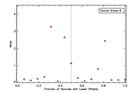
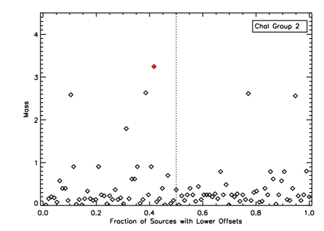
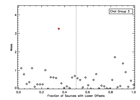
Figure 18: A continuation of Figure 17 showing the final two groups in Taurus and the groups in ChaI and Lupus3.

References

- Adams & Myers (2001) Adams, F. C., Myers, P. C. 2001, ApJ, 553, 744
- Allison et al (2009) Allison, R. J., Goodwin, S. P., Parker, R. J., de Grijs, R., Portegies Zwart, S. F., & Kouwenhoven, M. B. N. 2009, ApJ, 700, L99
- Ascenso et al (2009) Ascenso, J., Alves, J., & Lago, M. T. V. T. 2009, A&A, 495, 147
- Baraffe et al (1998) Baraffe, I., Chabrier, G., Allard, F., & Hauschildt, P. H. 1998, A&A, 337, 403
- Baraffe et al (2002) Baraffe, I., Chabrier, G., Allard, F., & Hauschildt, P. H. 2002, A&A, 382, 563
- Barrado et al (2009) Barrado, D., Morales-Calderón, M. Palau, A., Bayo, A., de Gregorio-Monsalvo, I., Eiroa, C., Huélamo, N., Buoy, H., Morata, O., & Schmidtobreick, L. 2009, A&A, 508, 859
- Barrow et al (1985) Barrow, J. D., Bhavsar, S., & Sonoda, D. H. 1985, MNRAS, 216, 17
- Bonnell & Davies (1998) Bonnell, I. A. & Davies, M. B. 1998, MNRAS, 295, 691
- Bonnell et al (2001) Bonnell, I. A., Clarke, C. J., Bate, M. R., & Pringle, J. E. 2001, MNRAS, 323, 785
- Bressert et al (2010) Bressert, E. Bastian, N., Gutermuth, R., Megeath, S. T., Allen, L., Evans, N. J. II, Rebull, L. M., Hatchell, J., Johnstone, D., Bourke, T. L., Cieza, L. A., Harvey, P. M., Merin, B., Ray, T. P., & Tothill, N. F. H. 2010, MNRAS, accepted (astroph 1009.1150)
- Carpenter et al (1997) Carpenter, J. M., Meyer, M. R., Dougados, C., Strom, S. E., & Hillenbrand, L. A. 1997, AJ, 114, 198
- Chabrier et al (2000) Chabrier, G., Baraffe, I., Allard, F., & Hauschildt, P. 2000, ApJ, 542, 464
- Chabrier (2005) Chabrier, G. 2005, The Initial Mass Function 50 years later, ed. Corbelli, E., Palla, F., & Zinnecker, H., ASSL, vol. 327, Springer Dordrecht, p.41
- Comerón et al (2003) Comerón, F., Fernàndez, M., Baraffe, I., Neuhäuser, R. & Kaas, A. A. 2003, A&A, 406, 1001
- Comerón (2008) Comerón, F. 2008, Handbook of Star Forming Regions, Volume II: The Southern Sky, ASP Monograph Publications, Vol. 5, ed. Bo Reipurth, p 295
- D’Antona & Mazzitelli (1994) D’Antona, F. & Mazzitelli, I. 1994, ApJS, 90, 467
- Dobashi et al (2005) Dobashi, K., Uehara, H., Kandori, R., Sakurai, T., Kaiden, M., Umemoto, T., & Sato, F. 2005, PASJ, 57, 1
- Elias, Alfaro, & Cabrera-Caño (2009) Elias, F., Alfaro, E. J., & Cabrera-Caño, J. 2009, MNRAS, 397, 2
- Elmegreen (2008) Elmegreen, B. G. 2008, ApJ, 672, 1006
- Evans et al (2009) Evans, N. J., Dunham, M. M., Jørgensen, J. K., Enoch, M. L., Merín, B., van Dishoeck, E. F., Alcalá, J. M., Myers, P. C., Stapelfeldt, K. R., Huard, T. L., Allen, L. E., Harvey, P. M., van Kempen, T., Blake, G. A., Koerner, D. W., Mundy, L. G., Padgett, D. L., Sargent, A. I. 2009, ApJS, 181, 321
- Feigelson & Babu (in prep) Feigelson, E. D. & Babu, G. J. Modern Statistical Methods for Astronomy with R Applications, text in prep
- Froebrich et al (2007) Froebrich, D., Murphy, G. C., Smith, M. D., Walsh, J., Del Burgo, C. 2007, MNRAS, 378, 1447
- Gomez et al (1993) Gomez, M., Hartmann, L., Kenyon, S. J., & Hewett, R. 1993, AJ, 105, 1927
- Gutermuth et al (2009) Gutermuth, R. A., Megeath, S. T., Myers, P. C., Allen, L. E., Pipher, J. L., & Fazio, G. G. 2009, ApJS, 184, 18
- Herbst (2008) Herbst, W. 2008, Handbook of Star Forming Regions: Volume I, The Northern Sky, ASP Monograph Publications, Vol.4, ed. Bo Reipurth, p372
- Hillenbrand (1997) Hillenbrand, L. 1997, AJ, 113, 1733
- Hillenbrand & Hartmann (1998) Hillenbrand, L. A. & Hartmann, L. W. 1998, ApJ, 492, 540
- Hughes et al (1994) Hughes, J., Hartigan, P., Krautter, J., & Kelemen, J. 1994, AJ, 108, 1071
- Jones & Herbig (1979) Jones, B. F. & Herbig, G. H. 1979, AJ, 84, 1872
- Jørgensen et al. (2008) Jørgensen, J. K., Johnstone, D., Kirk, H., Myers, P. C., Allen, L. E., & Shirley, Y. L. 2008, ApJ, 683, 822
- Kenyon et al (2008) Kenyon, S. J., Gómez, M. & Whitney, B. A. 2008, Handbook of Star Forming Regions, Volume I: The Northern Sky, ASP Monograph Publications, Vol. 4, ed Bo Reipurth, pp405
- Krautter et al (1997) Krautter, J., Wichmann, R., Schmitt, J. H. M. M., Alcalá, J. M., Neühauser, R., & Terranegra, L. 1997, A&AS, 123, 329
- Lada & Lada (2003) Lada, C. J. & Lada, E. A. 2003, ARA&A 41, 57
- Lada et al (2006) Lada, C. J., Muench, A. A., Luhman, K. L., Allen, A., Hartmann, L., Megeath, S. T., Myers, P., & Fazio, G. 2006, AJ, 131, 1574
- López Martí et al (2005) López Martí, B., Eislöffel, J. & Mundt, R. 2005, A&A, 440, 139
- Luhman et al (2003) Luhman, K. L. Stauffer, J. R., Muench, A. A., Rieke, G. H., Lada, E. A., Bouvier, J., & Lada, C. J. 2003, ApJ, 593, 1093
- Luhman (2004a) Luhman, K. L. 2004, ApJ, 602, 816
- Luhman (2004b) Luhman, K. L. 2004, ApJ, 614, 398
- Luhman et al (2005) Luhman, K. L., McLeod, K. K., & Goldenson, N. 2005, ApJ, 623, 1141
- Luhman (2007) Luhman, K. L. 2007, ApJS, 173, 104
- Luhman & Muench (2008) Luhman, K. L. & Muench, A. A. 2008, APJ, 684, 654
- Luhman et al (2008) Luhman, K. L., Allen, L. E., Allen, P. R., Gutermuth, R. A., Hartmann, L., Mamajek, E. E., Megeath, S. T., Myers, P. C., & Fazio, G. G. 2008, ApJ, 675, 1375
- Luhman (2008b) Luhman, K. L. 2008, Handbook of Star Forming Regions, Volume II: The Southern Sky, ASP Monograph Publications, Vol. 5, ed. Bo Reipurth, pp 169
- Luhman et al (2009) Luhman, K. L., Mamajek, E. E., Allen, P. R., & Cruz, K. L. 2009, ApJ, 703, 399
- Luhman et al (2010) Luhman, K. L., Allen, P. R., Espaillat, C., Hartmann, L., & Calvet, N. 2010, ApJS, 186, 111
- McKee & Tan (2003) McKee, C. F. & Tan, J. C. 2003, ApJ, 585, 850
- Maíz-Apellániz (2001) Maíz-Apellániz, J. 2001, ApJ, 563, 151
- Massi, Lorenzetti & Giannini (2003) Massi, F., Lorenzetti, D., & Giannini, T. 2003, A&A, 399, 147
- Merín et al (2008) Merín, B., Jørgensen, J., Spezzi, L., Alcalá, J. M., Evans, N. J. II, Harvey, P. M., Prusti, T., Chapman, N., Huard, T., can Dishoeck, E. F., & Comerón, F. 2008, ApJS, 177, 551
- Moeckel & Bonnell (2009) Moeckel, N. & Bonnell, I. A. 2009, MNRAS, 396, 1864
- Muench et al (2007) Muench, A. A. Lada, C. J., Muzerolle, J., & Young, E. 2007, AJ, 134, 411
- Myers (2009a) Myers, P. C. 2009, ApJ, 700, 1609
- Myers (2009b) Myers, P. C. 2009, ApJ, 706, 1341
- Nakajima et al (2000) Nakajima, Y., Tamura, M., Oasa, Y., & Nakajima, T. 2000, AJ, 119, 873
- Palla & Stahler (1999) Palla, F. & Stahler, S. 1999, ApJ, 525, 772
- Porras et al (2003) Porras, A., Christopher, M., Allen, L., Di Francesco, J., Megeath, S. T., & Myers, P. C. 2003, AJ, 126, 1916
- Rebull et al (2010) Rebull, L. M., Padgett, D. L., McCabe, C.-E., Hillenbrand, L. A., Stapelfeldt, K. R., Noriega-Crespo, A., Carey, S. J., Brooke, T., Huard, T., Tereby, S., Audard, M., Monin, J.-L., Fukagawa, M., Güdel, M., Knapp, G. R., Menard, F., Allen, L. E., Angione, J. R., Baldovin-Saavedra, C., Bouvier, J., Briggs, K., Dougados, C., Evans, N. J., Flagey, N., Guieu, S., Grosso, N., Glauser, A. M., Harvey, P., Hines, D., Latter, W. B., Skinner, S. L., Strom, S., Tromp, J., & Wolf, S. 2010, ApJS, 186, 259
- Reipurth (2008) Reipurth, B. 2008, Handbook of Star Forming Regions, Volumes I and II, ASP Monograph Publications, Vols 4, 5
- Rosolowsky et al (2008) Rosolowsky, E. W., Pineda, J. E., Kauffman, J., & Goodman, A. A. 2008, ApJ, 679, 1338
- Rowles & Froebrich (2009) Rowles, J., & Froebrich, D. 2009, MNRAS, 395, 1640
- Smith et al (2009) Smith, R., Longmore, S., & Bonnell, I. 2009, MNRAS, 400, 1775
- Stolte et al (2006) Stolte, A., Brandner, W., Brandl, B., & Zinnecker, H. 2006, ApJ, 132, 253
- Tan et al (2006) Tan, J. C., Krumholz, M. R., & McKee, C. F. 2006, ApJ, 641, L121
- Teixeira et al. (2005) Teixeira, P. S., Lada, C. J., & Alves, J. F. 2005, ApJ, 629, 276
- Testi et al (1999) Testi, L., Palla, F., & Natta, A. 1999, A&A, 342, 515
- Thé (1962) Thé, P. S. 1962, Contrib. Bosscha Obs., 15
- Torres et al (2007) Torres, R. A., Loinard, L., Mioduszewski, Am J., & Rodríguez, L. F.
- Walter et al (2003) Walter, F. M., Beck, T. L., Morse, J. A., & Wolk, S. J. 2003, AJ, 125, 2123
- Wang et al (2010) Wang, P., Li, Z.-Y., Abel, T., & Nakamura, F. 2010, ApJ, 709, 27
- Weidner et al (2010) Weidner, C., Kroupa, P., & Bonnell, I. A. D. 2010, MNRAS, 401, 275
- Zinnecker & Yorke (2007) Zinnecker, H. & Yorke, H. W. 2007, ARA&A, 45, 481