The low-momentum ghost dressing function and the gluon mass

Abstract:

We study both regular (the zero-momentum ghost dressing function not diverging), also named decoupling, and critical (diverging), also named scaling, Yang-Mills propagators solutions by analyzing the low-momentum behaviour of the ghost propagator Dyson-Schwinger equation (DSE) in Landau gauge, assuming for the truncation a constant ghost-gluon vertex, as it is extensively done, and a simple model for a massive gluon propagator. The asymptotic expression obtained for the regular or decoupling ghost dressing function up to the order ${\cal O}(q^{2})$ fits pretty well the low-momentum ghost propagator obtained through the numerical integration of the coupled gluon and ghost DSE in the PT-BFM scheme and, when the size of the coupling renormalized at some scale approaches some critical value, the PT-BFM results seems to trend to the the scaling solution as a limiting case.

1 Introduction

The low-momentum behaviour of the Yang-Mills propagators derived either from the tower of Dyson-Schwinger equations (DSE) or from Lattice simulations in Landau gauge has been a very interesting and hot topic for the last few years. It seems by now well established that, if we assume in the vanishing momentum limit a ghost dressing function behaving as $F(q^{2})\sim(q^{2})^{\alpha_{F}}$ and a gluon propagator as $\Delta(q^{2})\sim(q^{2})^{\alpha_{G}-1}$ (or, by following a notation commonly used, a gluon dressing function as $G(q^{2})=q^{2}\Delta(q^{2})\sim(q^{2})^{\alpha_{G}}$), two classes of solutions may emerge (see, for instance, the discussion of refs. [1, 2]) from the DSE: (i) those, dubbed “decoupling”, where $\alpha_{F}=0$ and the suppression of the ghost contribution to the gluon propagator DSE results in a massive gluon propagator (see [3, 4] and references therein); and (ii) those, dubbed “scaling”, where $\alpha_{F}\neq 0$ and the low-momentum behaviour of both gluon and ghost propagators are related by the coupled system of DSE through the condition $2\alpha_{F}+\alpha_{G}=0$ implying that $F^{2}(q^{2})G(q^{2})$ goes to a non-vanishing constant when $q^{2}\to 0$ (see [5, 6] and references therein).

Lattice QCD results appear to support only the massive gluon ($\alpha_{G}=1$) or scaling solutions (see [7, 8, 9, 10, 11, 12] and references therein), and also pinching technique results (see, for instance, [13, 21] and references therein), refined Gribov-Zwanziger formalism (see [15]) or other approaches like the infrared mapping of $\lambda\phi^{4}$ and Yang-Mills theories in ref. [16] or the massive extension of the Fadeev-Popov action in ref. [17] appear to point to.

In the present note, we briefly review the work of refs. [1, 2, 18], where it is established how both types of IR solutions for Landau gauge DSE emerge and how the transition between them may occur, and that of ref. [19] which extends the previous studies by the analysis of the results [20] obtained by solving the coupled system of Landau gauge ghost and gluon propagators DSE within the framework of the pinching technique in the background field method [21] (PT-BFM)

2 The two kinds of solutions of the ghost propagator Dyson-Schwinger equation

As was explained in detail in refs. [2, 18, 19], the low-momentum behavior for the Landau gauge ghost dressing function can be inferred from the analysis of the Dyson-Schwinger equation for the ghost propagator (GPDSE), which can be written diagrammatically as

$$\left(\begin{picture}(100.0,25.0)(0.0,0.0) \put(0.0,0.0){} \put(0.0,0.0){} \put(0.0,0.0){} \put(0.0,0.0){} \raise-10.0pt\hbox to0.0pt{\kern 12.5pt\makebox(0.0,0.0)[l]{a}\hss} \ignorespaces \raise-10.0pt\hbox to0.0pt{\kern 87.5pt\makebox(0.0,0.0)[r]{b}\hss} \ignorespaces \raise-10.0pt\hbox to0.0pt{\kern 50.0pt\makebox(0.0,0.0)[c]{k}\hss} \ignorespaces \end{picture}\right)^{-1}=\left(\begin{picture}(100.0,25.0)(0.0,0.0) \put(0.0,0.0){} \raise-10.0pt\hbox to0.0pt{\kern 12.5pt\makebox(0.0,0.0)[l]{a}\hss} \ignorespaces \raise-10.0pt\hbox to0.0pt{\kern 87.5pt\makebox(0.0,0.0)[r]{b}\hss} \ignorespaces \raise-10.0pt\hbox to0.0pt{\kern 50.0pt\makebox(0.0,0.0)[c]{k}\hss} \ignorespaces \end{picture}\right)^{-1}-\begin{picture}(150.0,25.0)(0.0,0.0) \put(0.0,0.0){} \put(0.0,0.0){} \put(0.0,0.0){} \put(0.0,0.0){} \put(0.0,0.0){} \put(0.0,0.0){} \put(0.0,0.0){} \put(0.0,0.0){} \put(0.0,0.0){} \put(0.0,0.0){} \put(0.0,0.0){} \put(0.0,0.0){} \put(0.0,0.0){} \raise-10.0pt\hbox to0.0pt{\kern 20.0pt\makebox(0.0,0.0)[l]{a,k}\hss} \ignorespaces \raise 15.0pt\hbox to0.0pt{\kern 50.0pt\makebox(0.0,0.0)[l]{d,$\nu$}\hss} \ignorespaces \raise-10.0pt\hbox to0.0pt{\kern 100.0pt\makebox(0.0,0.0)[l]{e}\hss} \ignorespaces \raise 15.0pt\hbox to0.0pt{\kern 100.0pt\makebox(0.0,0.0)[r]{f,$\mu$}\hss} \ignorespaces \raise-10.0pt\hbox to0.0pt{\kern 50.0pt\makebox(0.0,0.0)[l]{c,q}\hss} \ignorespaces \raise-10.0pt\hbox to0.0pt{\kern 120.0pt\makebox(0.0,0.0)[l]{b,k}\hss} \ignorespaces \raise 48.0pt\hbox to0.0pt{\kern 75.0pt\makebox(0.0,0.0)[c]{q-k}\hss} \ignorespaces \end{picture}\ ,$$ (1)

That analysis is performed on a very general ground: one applies the MOM renormalization prescription,

$$F_{R}(\mu^{2})\ =\ \mu^{2}\Delta_{R}(\mu^{2})\ =\ 1\ ,$$ (2)

where $\mu^{2}$ is the subtraction point, chooses for the ghost-gluon vertex,

$$\widetilde{\Gamma}_{\nu}^{abc}(-q,k;q-k)\ =\ ig_{0}f^{abc}\left(\ q_{\nu}H_{1}(q,k)+(q-k)_{\nu}H_{2}(q,k)\ \right)\ ,$$ (3)

to apply this MOM prescription in Taylor kinematics (i.e. with a vanishing incoming ghost momentum) and assumes the non-renormalizable bare ghost-gluon form factor, $H_{1}(q,k)=H_{1}$, to be constant in the low-momentum regime for the incoming ghost. Then, the low momentum-behaviour of the ghost dressing function and the gluon propagator is supposed to be well described by

$$\Delta_{R}(q^{2}) = \frac{B(\mu^{2})}{q^{2}+M^{2}}\ \simeq\frac{B(\mu^{2})}{M^{2}}\left(1-\frac{q^{2}}{M^{2}}+\cdots\right)\ ,$$ (4)

$$F_{R}(q^{2}) = A(\mu^{2})\left(\frac{q^{2}}{M^{2}}\right)^{\alpha_{F}}\left(1+\cdots\rule[0.0pt]{0.0pt}{17.07182pt}\right)\ ,$$ (5)

and one is finally left with:

$$F_{R}(q^{2})\simeq\left\{\begin{array}[]{lr}\displaystyle\left(\frac{10\pi^{2}}{N_{C}H_{1}g_{R}(\mu^{2})B(\mu^{2})}\right)^{1/2}\ \left(\frac{M^{2}}{q^{2}}\right)^{1/2}\ \left(1+\cdots\rule[0.0pt]{0.0pt}{17.07182pt}\right)&\mbox{\rm if}\ \alpha_{F}\neq 0\\ \displaystyle F_{R}(0)\left(1\ +\ \frac{N_{C}H_{1}}{16\pi}\ \overline{\alpha}_{T}(0)\ \frac{q^{2}}{M^{2}}\left[\ln{\frac{q^{2}}{M^{2}}}-\frac{11}{6}\right]\ +\ {\cal O}\left(\frac{q^{4}}{M^{4}}\right)\right)\rule[0.0pt]{21.33955pt}{0.0pt}\rule[14.22636pt]{0.0pt}{14.22636pt}&\mbox{\rm if}\ \alpha_{F}=0\end{array}\right.$$ (8)

where

$$\overline{\alpha}_{T}(0)=M^{2}\frac{g^{2}_{R}(\mu^{2})}{4\pi}F_{R}^{2}(0)\Delta_{R}(0).$$ (9)

It should be understood that the subtraction momentum for all the renormalization quantities is $\mu^{2}$. The case $\alpha_{F}\neq 0$ leads to the so-called scaling solution, where the low-momentum behavior of the massive gluon propagator forces the ghost dressing function to diverge at low-momentum through the scaling condition: $2\alpha_{F}+\alpha_{G}=0$ ($\alpha_{G}=1$ is the power exponent when dealing with a massive gluon propagator). As this scaling condition is verified, the perturbative strong coupling defined in this Taylor scheme [22], $\alpha_{T}=g_{T}^{2}/(4\pi)$, has to reach a constant at zero-momentum,

$$\alpha_{T}(0)\ =\frac{g^{2}(\mu^{2})}{4\pi}\lim_{q^{2}\to 0}q^{2}\Delta(q^{2})F(q^{2})F^{2}(q^{2})\ ,\ =\ \frac{5\pi}{2N_{C}H_{1}}$$ (10)

as can be obtained from Eqs.(4,8). The case $\alpha_{F}=0$ corresponds to the so-called decoupling solution, where the zero-momentum ghost dressing function reaches a non-zero finite value and eq. (8) provides us with the first asymptotic corrections to this leading constant. This subleading correction is controlled by the zero-momentum value of the coupling defined in eq. (9), which is an extension of the non-perturbative effective charge definition from the gluon propagator [23] to the Taylor ghost-gluon coupling [24]. As a consequence of the appropriate amputation of a massive gluon propagator, where the gluon mass scale is the same RI-invariant mass scale appearing in eq. (4), this Taylor effective charge is frozen at low-momentum and gives a non-vanishing zero-momentum value.

3 Comparison with numerical results from coupled DSE’s

We shall now compare the formulas given by eqs. (4,8) with some numerical results for the gluon propagator and ghost dressing function obtained by solving the coupled system of gluon and ghost DS equations obtained by applying the pinching technique in the background field method (PT-BFM) [21] (see also [14] and references therein). In the PT-BFM scheme for the coupled DSE system, the ghost propagator DSE is the same of Eq. (1), where the approximation $H_{1}=1$, and the gluon DSE is given by

$$\frac{(1+G(q^{2}))^{2}}{\Delta(q^{2})}\left(g_{\mu\nu}-\frac{q_{\mu}q_{\nu}}{q^{2}}\right)=q^{2}g_{\mu\nu}-q_{\mu}q_{\nu}+i\sum_{i=1}^{4}\left(a_{i}\right)_{\mu\nu}$$ (11)

where

$$a_{1}=\begin{picture}(112.5,18.75)(0.0,0.0) \put(0.0,0.0){} \put(0.0,0.0){} \put(0.0,0.0){} \put(0.0,0.0){} \put(0.0,0.0){} \put(0.0,0.0){} \put(0.0,0.0){} \put(0.0,0.0){} \put(0.0,0.0){} \put(0.0,0.0){} \put(0.0,0.0){} \put(0.0,0.0){} \put(0.0,0.0){} \end{picture}, a_{2}=\begin{picture}(112.5,18.75)(0.0,0.0) \put(0.0,0.0){} \put(0.0,0.0){} \put(0.0,0.0){} \put(0.0,0.0){} \put(0.0,0.0){} \put(0.0,0.0){} \put(0.0,0.0){} \put(0.0,0.0){} \end{picture}$$

$$a_{3}=\rule[0.0pt]{0.0pt}{42.67912pt}\begin{picture}(112.5,18.75)(0.0,0.0) \put(0.0,0.0){} \put(0.0,0.0){} \put(0.0,0.0){} \put(0.0,0.0){} \put(0.0,0.0){} \put(0.0,0.0){} \put(0.0,0.0){} \put(0.0,0.0){} \put(0.0,0.0){} \put(0.0,0.0){} \put(0.0,0.0){} \put(0.0,0.0){} \put(0.0,0.0){} \end{picture}, a_{4}=\begin{picture}(112.5,18.75)(0.0,0.0) \put(0.0,0.0){} \put(0.0,0.0){} \put(0.0,0.0){} \put(0.0,0.0){} \put(0.0,0.0){} \put(0.0,0.0){} \put(0.0,0.0){} \put(0.0,0.0){} \end{picture}.$$ (12)

where the external gluons are treated, from the point of view of Feynman rules, as background fields (these diagrams should be also properly regularized, as explained in [14]). The function $1+G$ defined in ref. [25] can be, in virtue of the ghost propagator DSE, connected to the ghost propagator [24]. The coupled system is to be solved, by numerical integration, with the two following boundary conditions as the only required inputs: the zero-momentum value of the gluon propagator and that of the coupling at a given perturbative momentum, $\mu=10$ GeV, that will be used as the renormalization point.

Thus, The PT-BFM framework leaves us with an attractive model for gluon and ghost propagators providing quantitative description of lattice data [4, 26] and giving well account of their main qualitative features: finite gluon propagator and finite ghost dressing function at zero-momentum. Futhermore, the coupled DSE system can be solved with different boundary conditions (see below).In particular, solutions obtained by keeping the zero-momentum value of the gluon propagator fixed (see lefthand plots of fig. 1) while $\alpha(\mu^{2}=100\mbox{\rm~{}GeV}^{2})$ is ranging from 0.15 to 0.1817 are available [20]. these solutions can be confronted to the asymptotical expressions derived in the previous section.

3.1 Decoupling solutions

Then, as the gluon propagator solutions in the PT-BFM scheme result to behave as massive ones, the eqs. (4,8) must account for the low-momentum behaviour of both gluon propagator and ghost dressing function with $H_{1}=1$ and $\overline{\alpha}_{T}(0)$ given by eq. (9), with $\alpha_{T}(\mu^{2})=g_{R}^{2}(\mu^{2})/(4\pi)$ being fixed, as a boundary condition for the numerical integration of the coupled DSE for each particular solution of the family (see tab. 1). Furthermore, the zero-momentum values of the ghost dressing function, $F_{R}(0)$ and of the gluon propagator, $\Delta_{R}(0)$, can be taken from the numerical solutions of the DSE (for any value of the $\alpha(\mu=10\mbox{\rm GeV})$). These altoghether with the gluon masses obtained by the fit of eq. (4) to the numerical DSE gluon propatator solutions (see the left plot in fig. 1, for $\alpha(\mu)=0.16$, and the results for $\alpha(\mu)=0.15,0.16,0.17$ in tab. 1, taken from ref. [19]), provide us with all the ingredients to evaluate, with no unknown parameter, eq. (8).

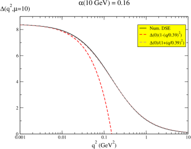
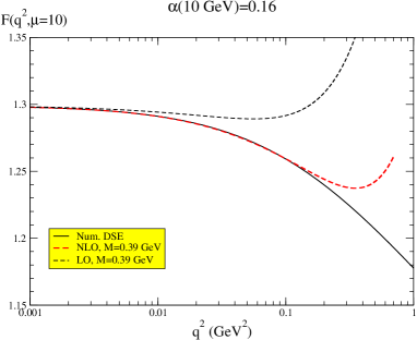
Figure 1: Gluon propagator (left) and ghost dressing function (right) after the numerical integration of the coupled DSE system for $\alpha(\mu=10\mbox{\rm GeV})=0.16$ taken from [20] . The curves for the best fits to gluon propagator and ghost propagator data explained in the text appear as red dotted lines. the same for the black dotted line in the lefthand plot but retaining only the logarithmic leading term for the asymptotic ghost dressing function by dropping the $-11/6$ away. In the righthand plots, the red dotted lines correspond to apply.

Indeed, the expression given by eq. (8) can be succesfully applied to describe the solutions all over the range of coupling values, $\alpha(\mu)$, at $\mu=10$ GeV (provided that they are not very close of the critical coupling that will be defined in the next subsection). This can be seen, for instance, for $\alpha=0.16$, in the right plots of fig. 1 and it is shown for $\alpha=0.15,0.16,0.17$ en ref. [19].

$\alpha(\mu)$	$\overline{\alpha}_{T}(0)$	$M$ (GeV) [gluon]
0.15	0.24	0.37
0.16	0.30	0.39
0.17	0.41	0.43

Table 1: Gluon masses and the zero-momentum non-perturbative effective charges, taken from ref. [19] and obtained as discussed in the text.

3.2 The “critical” limit

There appears to be a critical value of the coupling, $\alpha_{\rm crit}=\alpha(\mu^{2})\simeq 0.182$ with $\mu=10\mbox{\rm~{}Gev}$, above which the coupled DSE system does not converge any longer to a solution [20]. As a matter of the fact, we know from refs.[2, 19] that the scaling solution implies for the coupling

$$\alpha_{\rm crit}\ =\ \frac{g_{R}^{2}(\mu^{2})}{4\pi}\simeq\frac{5\pi^{2}}{2N_{C}A^{2}(\mu^{2})B(\mu^{2})}\ ,$$ (13)

where $B(\mu^{2})$ is determined by the gluon propagator solution that is supposed to behave as eq. (4), and $A(\mu^{2})$ by the ghost propagator that should behave as eq. (8) in the case $\alpha_{F}\neq 0$. Again, $\mu^{2}$ is the momentum at the subtraction point. This is also shown in ref. [1], where only the ghost propagator DSE with the kernel for the gluon loop integral is obtained from gluon propagator lattice data. In the analysis of ref. [1], a ghost dressing function solution diverging at vanishing momentum appears to exist and verifies eqs. (8,13), while regular or decoupling solutions exist for any $\alpha<\alpha_{\rm crit}$. In ref. [19], a more complete analysis is performed by studying again the dressing function computed by solving eq. (11) for the different values of the coupling, $\alpha=\alpha(\mu^{2})$, at $\mu^{2}=100$ GeV² [20]. The ghost dressing function at vanishing momentum, $F(0,\mu^{2})$, is described by the following power behaviour,

$$F(0)\ \sim\ (\alpha_{\rm crit}-\alpha(\mu^{2}))^{-\kappa(\mu^{2})}\ ,$$ (14)

where $\kappa(\mu^{2})$ is a critical exponent (depending presummably on the renormalization point, $\mu^{2}$), supposed to be positive and to govern the transition from decoupling ($\alpha<\alpha_{\rm crit}$) to the scaling ($\alpha=\alpha_{\rm crit}$) solutions; and where we let $\alpha_{\rm crit}$ be a free parameter to be fitted by requiring the best linear correlation for $\log[F(0)]$ in terms of $\log[\alpha_{\rm crit}-\alpha]$. In doing so, the best correlation coefficient is 0.9997 for $\alpha_{\rm crit}=0.1822$, which is pretty close to the critical value of the coupling above which the coupled DSE system does not converge any more, and $\kappa(\mu^{2})=0.0854(6)$. This can be seen in fig. 2.(a), where the log-log plot of $F_{R}(0)$ in terms of $\alpha_{\rm crit}-\alpha$ is shown and the linear behaviour with negative slope corresponding to the best correlation coefficient strikingly indicates a zero-momentum ghost propagator diverging as $\alpha\to\alpha_{\rm crit}$. Nevertheless, no critical or scaling solution appears for the coupled DSE system in the PT-BFM, although the decoupling solutions obtained for any $\alpha<\alpha_{\rm crit}=0.1822$ seem to approach the behaviour of a scaling one when $\alpha\to\alpha_{\rm crit}$. The absence of the scaling solution in the PT-BFM approach can be well understood by analysing eq. (11) as explained in ref. [19].

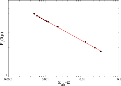
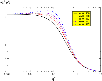
(a)	(b)

Figure 2: (a) Log-log plot of the zero-momentum values of the ghost dressing function, obtained by the numerical integration of the coupled DSE system in the PT-BFM scheme, in terms of $\alpha_{\rm crit}-\alpha$. $\alpha=\alpha(\mu=10\mbox{\rm GeV})$, the value of the coupling at the renormalization momentum, is an initial condition for the integration; while $\alpha_{\rm crit}$ is fixed to be 0.1822, as explained in the text, by requiring the best linear correlation. (b) Gluon propagator solutions in terms of $q^{2}$ for the same coupled DSE system for different values of $\alpha(\mu=10\mbox{\rm GeV})$, all very close to the critical value, ranging from 0.18 to 0.1817 .

When approaching the critical value of the coupling, the gluon propagators obtained from the coupled DSE system in PT-BFM must be also thought to obey the same critical behaviour pattern as the ghost propagator. In the PT-BFM, the value at zero-momentum being fixed by construction [4, 20], one should expect that, instead of decreasing, the gluon propagator obtained for couplings near to the critical value increases for low momenta: the more one approaches the critical coupling the more it has to increase. This is indeed the case, as can be seen in fig. 2(b). This also implies that, near the critical value, the low momentum propagator does not obey eq. (4) and that consequently eq. (8) does not work any longer to describe the low momentum ghost propagator.

4 Conclusions

The ghost propagator DSE, with the only assumption of taking $H_{1}(q,k)$ from the ghost-gluon vertex in eq. (3) to be constant in the infrared domain of $q$, can be exploited to look into the low-momentum behaviour of the ghost propagator. The two classes of solutions named “decoupling” and “scaling” can be indentified and shown to depend on whether the ghost dressing function achieves a finite non-zero constant ($\alpha_{F}=0$) at vanishing momentum or not ($\alpha_{F}\neq 0$). The solutions appear to be dialed by the size of the coupling at the renormalization momentum which plays the role of a boundary condition for the DSE integration.

We applied a model with a massive gluon propagator to obtain the low-momentum behaviour of the ghost propagator that results to be regulated by the gluon mass and by a regularization-independent dimensionless quantity that appears to be the effective charge defined from the Taylor-scheme ghost-gluon vertex at zero momentum. Then, we demonstrated that the asymptotic decoupling formula ($\alpha_{F}=0$) successfully describes the low-momentum ghost propagator computed trhough the numerical integration of the coupled gluon and ghost DSE in the PT-BFM scheme. We also show that the zero-momentum ghost dressing function tends to diverge when the value of the coupling dialing the solutions approaches some critical value. Such a divergent behaviour at the critical coupling corresponds to a scaling solution where, if the gluon is massive, $\alpha_{F}=-1/2$.

Acknowledgements: The author acknowledges the Spanish MICINN for the support by the research project FPA2009-10773 and “Junta de Andalucia” by P07FQM02962.

References

- [1] Ph. Boucaud, J. P. Leroy, A. L. Yaouanc, J. Micheli, O. Pene and J. Rodriguez–Quintero, JHEP 0806 (2008) 012 arXiv:0801.2721 [hep-ph].
- [2] Ph. Boucaud, J. P. Leroy, A. Le Yaouanc, J. Micheli, O. Pene and J. Rodriguez-Quintero, JHEP 0806 (2008) 099 [arXiv:0803.2161 [hep-ph]].
- [3] A. C. Aguilar and J. Papavassiliou, JHEP 0612 (2006) 012; Eur. Phys. J. A 31 (2007) 742; A. C. Aguilar and A. A. Natale, JHEP 0408 (2004) 057.
- [4] A. C. Aguilar, D. Binosi and J. Papavassiliou, Phys. Rev. D 78 (2008) 025010 [arXiv:0802.1870 [hep-ph]].
- [5] R. Alkofer and L. von Smekal, Phys. Rept. 353 (2001) 281 [arXiv:hep-ph/0007355]; C. Lerche and L. von Smekal, Phys. Rev. D 65 (2002) 125006 [arXiv:hep-ph/0202194]; D. Zwanziger, Phys. Rev. D 65 (2002) 094039 [arXiv:hep-th/0109224]; C. S. Fischer and R. Alkofer, Phys. Lett. B 536 (2002) 177 [arXiv:hep-ph/0202202]; J. M. Pawlowski, D. F. Litim, S. Nedelko and L. von Smekal, Phys. Rev. Lett. 93 (2004) 152002 [arXiv:hep-th/0312324]. M. Q. Huber, R. Alkofer, C. S. Fischer and K. Schwenzer, Phys. Lett. B 659 (2008) 434 [arXiv:0705.3809 [hep-ph]].
- [6] C. S. Fischer, A. Maas and J. M. Pawlowski, Annals Phys. 324 (2009) 2408 [arXiv:0810.1987 [hep-ph]].
- [7] A. Cucchieri and T. Mendes, PoS LAT2007 (2007) 297 [arXiv:0710.0412 [hep-lat]]; Phys. Rev. Lett. 100 (2008) 241601 [arXiv:0712.3517 [hep-lat]]; arXiv:0904.4033 [hep-lat];
- [8] I. L. Bogolubsky, E. M. Ilgenfritz, M. Muller-Preussker and A. Sternbeck, Phys. Lett. B 676 (2009) 69 [arXiv:0901.0736 [hep-lat]]; I. L. Bogolubsky, E. M. Ilgenfritz, M. Muller-Preussker and A. Sternbeck, PoS LAT2007 (2007) 290 [arXiv:0710.1968 [hep-lat]].
- [9] A. Sternbeck, E.-M. Ilgenfritz, M. M uller-Preussker and A. Schiller, Nucl. Phys. Proc. Suppl. 140 (2005) 653; AIP Conference Proceedings 756 (2005) 284, [arXiv:hep-lat/0412011].
- [10] P. Boucaud et al., [arXiv:hep-ph/0507104 ].
- [11] O. Oliveira and P. Bicudo, arXiv:1002.4151 [hep-lat]; D. Dudal, O. Oliveira and N. Vandersickel, Phys. Rev. D 81 (2010) 074505 [arXiv:1002.2374 [hep-lat]].
- [12] V. G. Bornyakov, V. K. Mitrjushkin and M. Muller-Preussker, Phys. Rev. D 81 (2010) 054503 [arXiv:0912.4475 [hep-lat]].
- [13] J. M. Cornwall, Phys. Rev. D 26, 1453 (1982).
- [14] D. Binosi and J. Papavassiliou, Phys. Rept. 479 (2009) 1 [arXiv:0909.2536 [hep-ph]].
- [15] D. Dudal, S. P. Sorella, N. Vandersickel and H. Verschelde, arXiv:0711.4496 [hep-th]; D. Dudal, J. A. Gracey, S. P. Sorella, N. Vandersickel and H. Verschelde, Phys. Rev. D 78 (2008) 065047 [arXiv:0806.4348 [hep-th]].
- [16] M. Frasca, Phys. Lett. B 670 (2008) 73 [arXiv:0709.2042 [hep-th]].
- [17] M. Tissier and N. Wschebor, arXiv:1004.1607 [hep-ph].
- [18] Ph. Boucaud, M. E. Gomez, J. P. Leroy, A. L. Yaouanc, J. Micheli, O. Pene and J. Rodriguez-Quintero, Phys. Rev. D 82 (2010) 054007 [arXiv:1004.4135 [hep-ph]]
- [19] J. Rodriguez-Quintero, [arXiv:1005.4598 [hep-ph]].
- [20] A. C. Aguilar, Private communication.
- [21] D. Binosi and J. Papavassiliou, Phys. Rev. D 66 (2002) 111901 [arXiv:hep-ph/0208189]; Phys. Rev. D 77 (2008) 061702 [arXiv:0712.2707 [hep-ph]]; D. Binosi and J. Papavassiliou, Phys. Rev. D 77 (2008) 061702 [arXiv:0712.2707 [hep-ph]].
- [22] Ph. Boucaud, F. De Soto, J. P. Leroy, A. Le Yaouanc, J. Micheli, O. Pene and J. Rodriguez-Quintero, Phys. Rev. D 79 (2009) 014508 [arXiv:0811.2059 [hep-ph]]; A. Sternbeck, K. Maltman, L. von Smekal, A. G. Williams, E. M. Ilgenfritz and M. Muller-Preussker, PoS LAT2007 (2007) 256 [arXiv:0710.2965 [hep-lat]].
- [23] A. C. Aguilar, D. Binosi and J. Papavassiliou, PoS LC2008 (2008) 050 [arXiv:0810.2333 [hep-ph]].
- [24] A. C. Aguilar, D. Binosi, J. Papavassiliou and J. Rodriguez-Quintero, Phys. Rev. D 80 (2009) 085018 [arXiv:0906.2633 [hep-ph]].
- [25] D. Binosi and J. Papavassiliou, Phys. Rev. D 66 (2002) 025024 [arXiv:hep-ph/0204128]; P. A. Grassi, T. Hurth and M. Steinhauser, Annals Phys. 288 (2001) 197 [arXiv:hep-ph/9907426].
- [26] A. C. Aguilar, D. Binosi and J. Papavassiliou, JHEP 1007 (2010) 002. arXiv:1004.1105 [hep-ph]. ….